Abstract
This work aims to improve the reliability of dynamic systems by eliminating the effect of random control variables. At first, the reliability-based dynamic optimization problem (RB-DOP) is introduced and defined to account for dynamic systems with uncertainty associated with random control variables. Whereafter, in order to solve RB-DOP efficiently, the constraint function response shift scalar (CFRSS)-based RB-DOP optimization method is proposed, in which the nested RB-DOP is decoupled into an equivalent deterministic DOP and a CFRSS search problem, and the two problems are addressed iteratively until the control law converges. Specifically, the shift scalar CFRSS is calculated by the probability density function of the constraint function response and deducted for probabilistic constraints in the constraint function response space to move the violated constraints toward the reliable region, avoiding solving large-scale optimization problems in the control variable space. Finally, two numerical examples and a low-thrust orbit transfer problem are investigated to demonstrate the feasibility of the proposed approach.
Keywords:
dynamic system; reliability-based dynamic optimization; random control variable; constraint function response shift scalar MSC:
93-08
1. Introduction
In a dynamic system containing control inputs, the state trajectory of the system evolves with the control law according to the dynamic properties, and the system performance indicator also depends on the control law. The dynamic optimization problem (DOP), also referred to as the optimal control problem, is a popular class of optimization problems in control theory for searching the optimal control laws of nonlinear dynamic systems [1,2]. In DOP, the dynamical equation (i.e., state equation) describing the dynamic properties of a system is represented by differential algebraic equations, and the optimal control law is available by optimizing the performance indicator [3]. Pontryagin’s maximum principle [4] and the dynamic programming principle [5], as the conventional analytical methods, can hardly yield the desired open-loop control law for DOP due to the increasing complexity and nonlinearity of dynamic systems, as well as the constraints imposed by practical engineering. Consequently, with improvements in computer performance, various numerical methods, such as indirect and direct methods, have been widely investigated [6,7,8,9,10]. Among those numerical methods, the direct method is extensively adopted in engineering practices on account of its capability to efficiently solve DOPs containing inequality constraints [11,12,13]. When solving DOP by the direct method, the infinite-dimensional DOP is transformed into a finite-dimensional nonlinear programming problem (NLP) [14], then NLP is addressed by the gradient-based optimization algorithms (e.g., sequential quadratic programming [15]) to obtain the optimal DOP solution.
The above DOP methods have been successfully deployed in a deterministic manner to dynamic systems. However, uncertainties widely exist in engineering practice, e.g., changing environmental conditions and manufacturing tolerances [16,17]. Thus, the control law from the controller may not be a deterministic desired curve but one with random uncertainty at all time nodes. Meanwhile, it is widely known that deterministic optimization typically pushes a design to the limits of the constraints, allowing little or no space for uncertainty. As a consequence, the above deterministic DOP methods may generate unreliable control decisions, which can reduce the reliability of dynamic systems and even cause security accidents.
To the best knowledge of the authors, although some adaptive control methods have been proposed to manage system uncertainties [18,19], there has been little relevant research on the quantitative analysis of the reliability of dynamic systems and the search for reliable and optimal control laws considering the randomness of control variables. However, in static systems, the random uncertainty of design variables has been extensively researched in the reliability-based design optimization (RBDO) problem to improve static system reliability [20,21,22,23,24,25,26]. In the standard RBDO formulation, the random uncertainty of design variables propagates through inequality constraints and affects a system’s reliability, and the failures caused by the random design variables can be quantified by the probability of failure [27,28,29]. The reliability index approach [30,31] and the performance measurement approach [32] are two conventional double-loop methods for RBDO, in which the outer loop optimizes the design variables and the inner loop analyzes the random uncertainty. Nevertheless, the reliability analysis of the inner loop is nested in the deterministic optimization of the outer loop, leading to the double-loop methods being computationally expensive. To improve solving efficiency, decoupled-loop methods have been used for RBDO. The representative and promising method belonging to decoupled-loop methods is sequential optimization and reliability assessment (SORA) [33,34,35,36,37,38], in which the RBDO problem is decomposed into deterministic optimization and reliability assessment subproblems, the shift vector calculated in the reliability assessment is passed to deterministic optimization, and the shift vector is deducted for each probabilistic constraint in the design variable space to move the violated constraints toward the reliable region in deterministic optimization. Different from deducting the shift vector in the design variable space, Jiang et al. [39] proposed a probability density function (PDF)-based performance shift approach (PPSA), in which the shift scalar is deducted for each probabilistic constraint in the response space to move the violated constraints toward the reliable region in deterministic optimization. Compared to the sequential RBDO methods, PPSA enhances computational efficiency.
Motivated by the advantage that the PPSA method can effectively deal with RBDO in static systems, this paper aims to define the reliability-based dynamic optimization problem (RB-DOP) with random control variables and to propose a corresponding effective optimization method developed from the static PPSA method. This work contributes to eliminating the adverse impact of random control variables on dynamic system performance and satisfying the higher requirement of dynamic system reliability. The main contributions of this paper are as follows.
1. Different from the research about DOP and RBDO, this work introduces a more challenging RB-DOP into dynamic systems to account for the random uncertainty stemming from control variables. In this paper, the RB-DOP is defined by assigning random uncertainty to control variables at all time nodes. As time evolves, the random uncertainty of control variables propagates not only through inequality constraints but also through the state equations of a dynamic system and has an impact on the state trajectories and the reliability of the dynamic system over the time domain.
2. The current PPSA method is only suited to solving RBDO in static systems. Meanwhile, the SORA method needs to calculate shift scalars of lots of discrete design variables when solving RB-DOP, which increases the complexity and computational effort. In contrast, this article presents the concept of the constraint function response shift scalar (CFRSS) and proposes the CFRSS-based RB-DOP optimization method. The CFRSS is a shift scalar that is calculated according to approximate PDFs. It acts on the constraint function response space, rather than on the control variable space, to move the violated constraints toward the reliable region. Therefore, the proposed method greatly improves the computational efficiency of RB-DOP with random control variables.
The remainder of this paper is organized in the following manner: A brief introduction is given to DOP and the RBDO problem in Section 2. The formulation and implementation of the CFRSS-based RB-DOP solving method are elaborated in Section 3. Two numerical examples and an engineering application are investigated in Section 4 to demonstrate the feasibility of the proposed method. Finally, the conclusion is summarized in Section 5.
2. Related Work
2.1. Dynamic Optimization Problem and Direct Transcription Method
The general form of DOP is described as follows:
where and are mean state variables and control variables, respectively; and are the design spaces of and ; and indicate the initial and terminal states of the dynamic system at the initial time and terminal time; the objective function consists of the Mayer term, , and the Lagrange term, ; and is the integrand function of the Lagrange term. DOP is subject to the state equation formulated by the algebraic differential equations; the boundary constraint, ; and the inequality constraint function, . The state equation and path constraint are continuous constraints that must be satisfied throughout the time period , while the boundary constraint is the discrete constraint that should only be satisfied at the time nodes and .
The direct transcription method [40] is a “discretize-then-optimize” approach for DOP, in which state variables, , and control variables, , are discretized at the time grid nodes . These discrete state and control variables compose the state matrix, , and the control matrix, . Then, the infinite-dimensional DOP is transcribed into a large sparse finite-dimensional NLP expressed by
where the elements in are treated as new design variables in this NLP, are the weights specific to the quadrature method, and are the defect constraints constructed from state equation and have to be added at each time node to ensure the continuity of the state trajectories and control curves. And the detailed transcription process is available in Ref. [41].
2.2. Reliability-Based Design Optimization and the SORA Method
In a static system, the RBDO formulation can be expressed as follows:
where denotes the vector of random design variables; are the mean values of and can be treated as the deterministic design variables; and are the lower bound and upper bound of , respectively; is the objective function; stands for the actual reliability of the constraint function, ; and and are the desired design probability and the target reliability level of .
SORA, as the representative and promising solving method for RBDO, decouples RBDO into deterministic optimization and reliability assessment. The deterministic optimization is given as
where is the shift vector in the iteration and is deducted for the probabilistic constraint in the design variable space to move the violated constraints toward the reliable region. is the minimum performance target point, and its corresponding point, , in the standard normal space (U-space) can be calculated in the reliability assessment optimization problem [32].
3. The Constraint Function Response Shift Scalar-Based RB-DOP Optimization Method
To describe the effect of random control variables on dynamic system performance, the general formulation of RB-DOP is defined first in this section. Then, the concept of CFRSS is proposed by analyzing the SORA method in RBDO. Furthermore, a CFRSS-based RB-DOP optimization method is developed, which decouples the RB-DOP into an equivalent deterministic DOP and a CFRSS search problem. Finally, the specific implementation procedure of the CFRSS-based RB-DOP optimization method is demonstrated in detail.
3.1. Reliability-Based Dynamic Optimization Problem
The general formulation of RB-DOP is defined as
where the vectors and represent random control variables and state variables; the vectors and stand for the mean values of and , respectively; and the uncertainty of depends on both and the state equation . In addition, RB-DOP is also subject to the probability constraint , where denotes the actual reliability of the constraint function and is the desired design probability.
In RBDO, the vector of random design variable can be seen as a multi-dimensional design point, and the uncertainty of is described by assuming that follows the normal distribution , while the random control variables, , in RB-DOP are time-dependent curves whose values vary continuously throughout the time period . This means that the uncertainty of exists at all time nodes . To deal with the uncertainty of the random control variables, , they are discretized on the time axis. Meanwhile, to facilitate the formula description of related concepts, the random control variables at any time node are assumed to follow normal distributions , while other types of random distributions can also be handled in this article. As shown in Figure 1a, the red line is the deterministic control curve and the green line is one of the random control curves generated by assigning uncertainty to the deterministic control curve at the time nodes. The green region in Figure 1b consists of a collection of random control curves, which means that if the ideal control curve is the red line, the real control curve will be any of the curves in the green region.
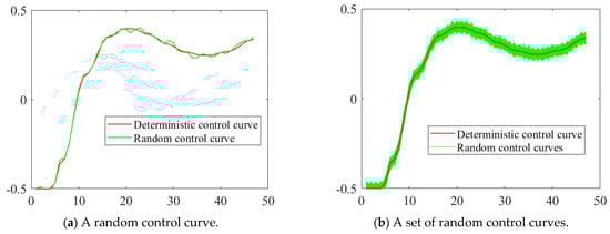
Figure 1.
Deterministic and random control curves.
When solving RB-DOP by the direct transcription method, the state variables, , and control variables, , are discretized at the time grid nodes as and , and the elements in are treated as new design variables in NLP. Besides the defect constraints in Equation (4) that ensure the continuity of the state trajectories and control curves, reliability analysis should also be performed at all time nodes to ensure that the design variables at the time nodes satisfy the probability constraints. That is, the probability constraints in Equation (5) are transformed into
where stands for the probability constraint enforced on the design variables at the time node , and its specific expression is as follows:
However, as the solving process proceeds iteratively, the time nodes grow denser, leading to more and more elements in the design variables . When solving RB-DOP based on the SORA method from the perspective of design variables , large-scale defect constraints and probability constraints need to be handled, which definitely increases the complexity and computational effort and even makes RB-DOP unsolvable. Therefore, an efficient RB-DOP optimization method deserves to be investigated.
3.2. The Constraint Function Response Shift Scalar
Reviewing the deterministic optimization in SORA, the inequality constraint in Equation (2) can be rewritten as
where the shift vector is known and denotes the constraint function response shift scalar of and can be treated as a function, in which is the independent variable and the response of is the dependent variable. It is important to notice that, in general, there is a one-to-one correspondence between and at the current optimal design points (i.e., suboptimal or optimal design points) in RBDO, which means that once the current optimal design, , is determined, the current response of is also determined.
Let be denoted as , then
where is a scalar and the reduced form of in this work. Since and correspond one-to-one at the current optimal design points in the general RBDO, once the current CFRSS is given, the corresponding can be obtained through the deterministic optimization in Equation (4). From Equation (9), it can be observed that is deducted for the probabilistic constraint in the constraint function response space, rather than in the design variable space, to move the violated constraint toward the reliable region.
Similarly, the inequality constraint in RB-DOP can be written as
And at time nodes, the inequality constraint is rewritten as
where and (i.e., ) correspond one-to-one with the help of the objective function and other constraints in RB-DOP, and once the current optimal CFRSS has been given, the corresponding (i.e., ) also can be determined by the direct transcription method. Therefore, in Equations (10) and (11) acts on the constraint function response space, rather than on the state-control variable space.
Obviously, the scale of design variables in large-scale NLP transformed from RB-DOP increases with the density of the time grid nodes during the solving process, which leads to the number of equation constraints and reliability constraints increasing dramatically. Therefore, it is not wise to solve RB-DOP by the shift vector in the state-control variable space. Fortunately, CFRSS is a scalar and corresponds to in RB-DOP. To this end, it is a feasible strategy to optimize RB-DOP through CFRSS in the constraint function response space. Based on this idea, the CFRSS-based RB-DOP optimization method is proposed in a later section.
3.3. The CFRSS-Based RB-DOP Optimization Method
The RB-DOP model in Equation (5) can be expressed in the form of a PDF as
where is the response of the inequality constrain, , and is the PDF of when the mean values of the state and control variables are . In Equation (12), the probability constraint becomes a one-dimensional integral of the PDF of , and the reliability can be calculated by .
The CFRSS-based RB-DOP optimization method treats the response of as a starting point, translates the RB-DOP into an equivalent deterministic DOP and a CFRSS searching problem, and solves those two problems iteratively until the convergence condition is satisfied.
3.3.1. Formulate an Equivalent Deterministic DOP
The equivalent deterministic DOP based on CFRSS is as follows:
where is the CFRSS and the inequality constraint is shifted towards the reliable region by such that the design variables generated by solving the equivalent deterministic DOP satisfy the original probability constraint in Equation (5).
3.3.2. Search for the Constraint Function Response Shift Scalar
To more clearly illustrate the search process for the constraint function response shift scalar, the PDF of the constraint function response for design variables is defined as . Moreover, can be provided by the fitting procedure introduced in Section 3.3.3.
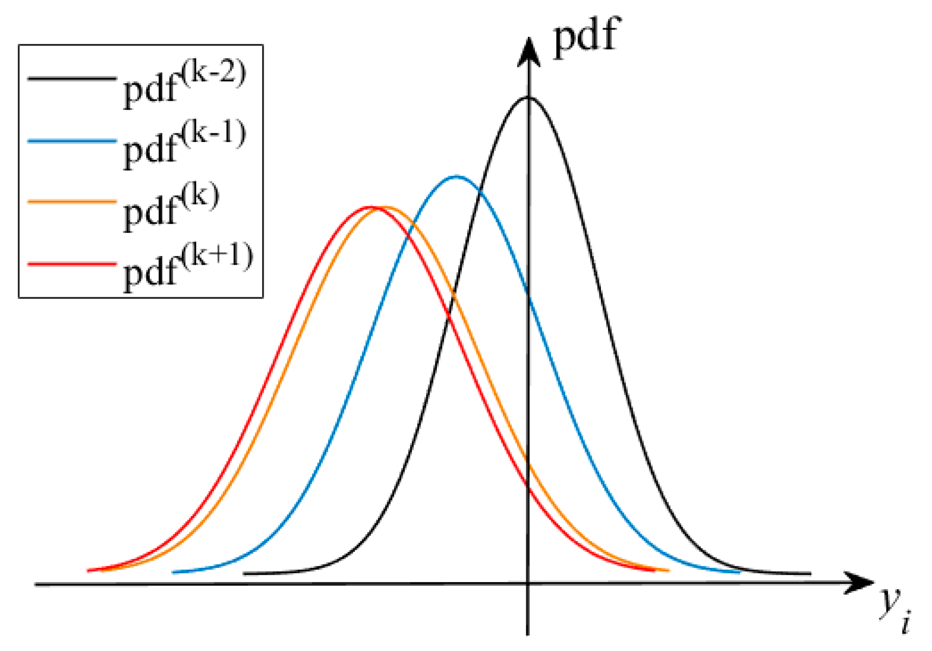
Figure 2 plots the response PDFs at sequential iterations; it can be found that gradually converges and tends to coincide as the solution proceeds, i.e., the mean values and dispersions of in the iterations tend to be the same, especially in the and iterations of the late iteration stage. Note that once the mean value of the constraint function response is given, the search for the optimal mean values of state and control variables is transformed into a DOP problem that has a unique optimal solution because of the limitations imposed by the optimality of the objective function in the DOP problem. That means that the dispersion of can be considered as varying with . Therefore, it is reasonable to assume that only the location of the mean value moves by from in the iteration to in the iteration. Based on this assumption, the PDF in the iteration can be described by the PDF in the iteration, and can be given as
where represents the constraint function response shift distance that moves when the design variables are updated from to .
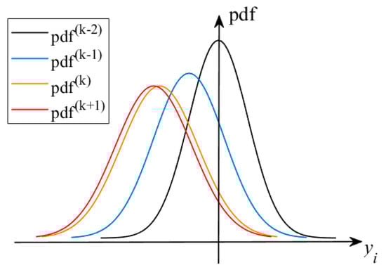
Figure 2.
Diagram of response PDFs at sequential iterations.
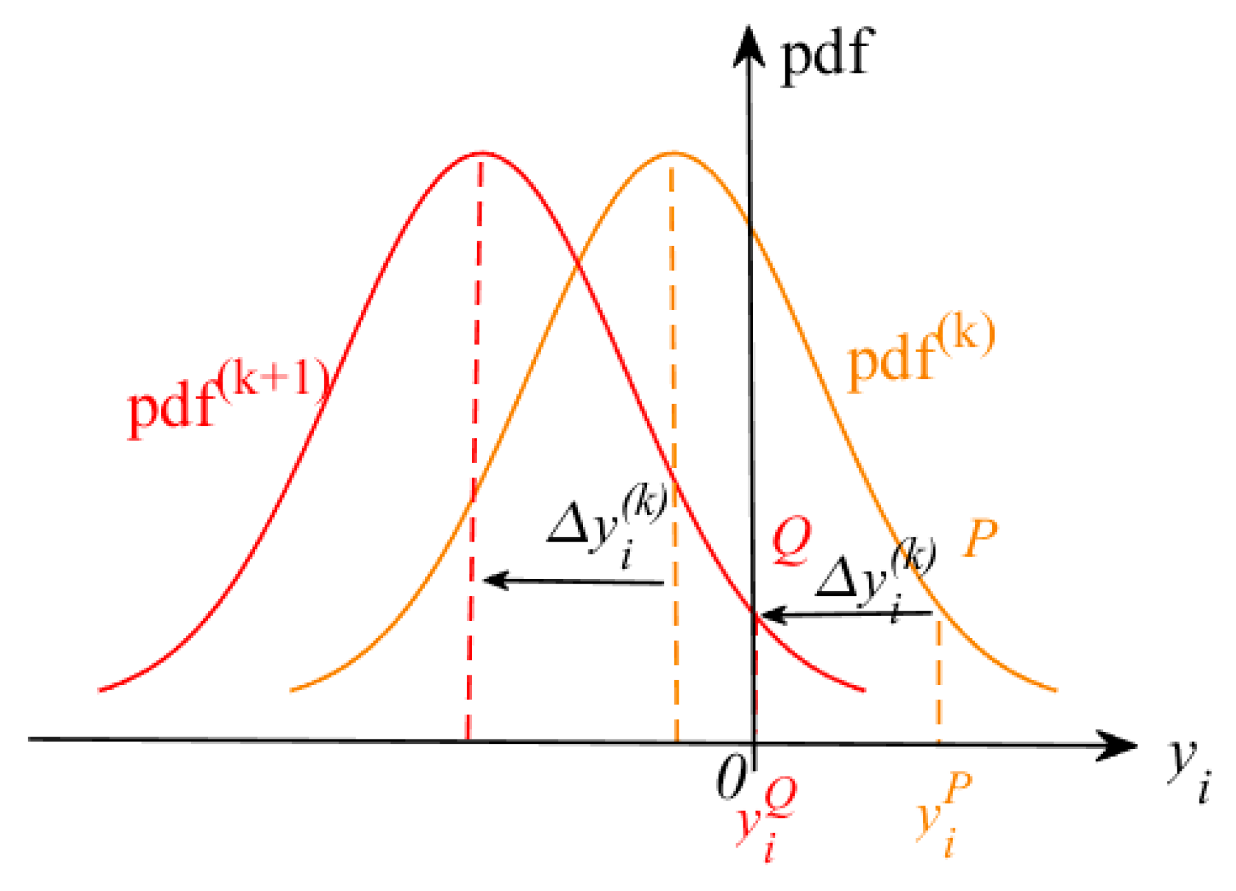
To search for CFRSS , the analysis of the constraint function response shift distance, , in Equation (14) is performed based on the PDF . Geometrically, as can be observed from Figure 3, point is located on the PDF in the iteration, the constraint function response at point is , and . To ensure that in the iteration, it is necessary to shift by in the direction of enhancing reliability, i.e., the negative direction of the horizontal coordinate, to obtain . Correspondingly, point moves to point , and the constraint function response at point is 0. The distance, , that the constraint function response moves horizontally in the iterations can be expressed as
where because of the negative direction of the horizontal coordinate.
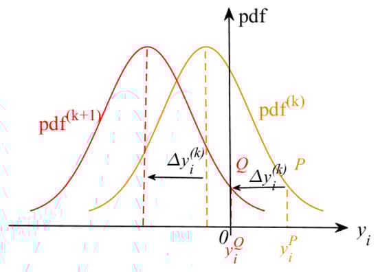
Figure 3.
Schematic diagram of the convergence of the PDF of .
Mathematically, in the PDF-based RB-DOP formulation in Equation (12), the probability constraint is
Substituting Equation (14) into Equation (16) yields
where the PDF of the constraint function response is obtained in the iteration. Hence, the integral term in Equation (17) can be regarded as a function of .
Furthermore, Equation (18) can be abbreviated as
Then, the constraint function response shift distance, , can be solved by the inverse function of .
Combining Equations (15) and (20) yields
That is,
By comparing the inequality constraint in Equations (13) and (22), CFRSS can be calculated by
It is noteworthy that when the initial value, , of is the solution of , i.e.,
we notice that the latest iterative solution, , typically locates on constraint boundaries, as in Equation (22) of the current optimization problem, i.e.,
Finally, CFRSS can be calculated by
3.3.3. Fit the PDF of the Constraint Function Response
As mentioned earlier, the PDF of the constraint function response is the basis for calculating CFRSS . To obtain efficiently, a fitting procedure for has been developed based on the Monte Carlo method and the Johnson distribution. For simplicity, the basics of the Johnson distribution can be found in Appendix A. The specific steps of the fitting procedure are listed as follows:
Step 1: Generate the control sample set (i.e., the training sample dataset) . Using the current optimal control variables as the mean values, The containing random control curves, are generated in the feasible domain according to the definition of the random control variables.
where is formed by connecting the discrete points in .
Step 2: Calculate the constraint function response set, , corresponding to . Feed elements in into the constraint function, , to obtain containing values of the constraint function response, .
- If the constraint function, , does not contain state variables , then
- If the constraint function, , contains state variables , the state trajectory sample set of is first calculated based on the state equations and using the Runge–Kutta algorithm, then
Note that when involves , the value of is a set of time series . Considering that the largest element, , in is most likely to violate the constraint , is treated as the value of constraint function response .
Step 3: Fit the PDF. The appropriate Johnson distribution type is selected to fit by the category identification criterion according to the distribution characteristic of the elements in , and then the parameters in the Johnson distribution are estimated using the percentile matching method to approximate the PDF of .
3.4. The Implementation Process of the CFRSS-Based RB-DOP Optimization Method
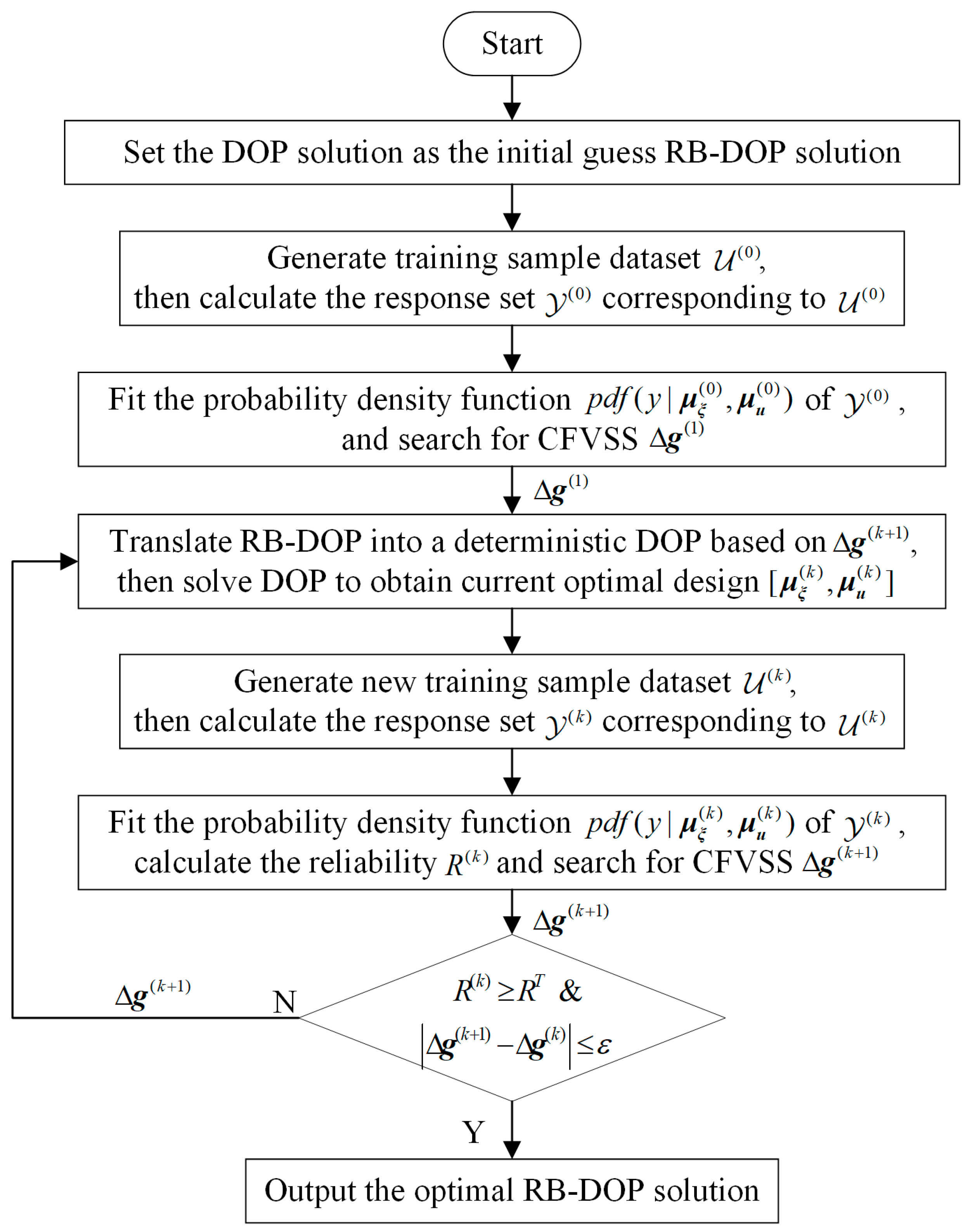
As discussed above, the proposed CFRSS-based RB-DOP optimization method decouples RB-DOP into an equivalent deterministic DOP and a CFRSS search problem, the deterministic DOP is optimized using the direct transcription technique, and the CFRSS search problem is solved based on the PDF of the constraint function response, , fitted by the Monte Carlo method and the Johnson distribution. The flowchart of the CFRSS-based RB-DOP optimization method is shown in Figure 4, and the specific implementation procedure is elaborated as follows.
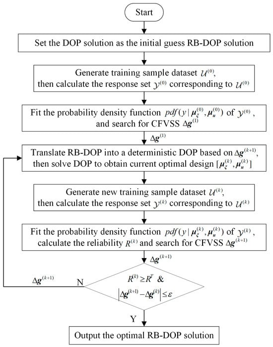
Figure 4.
Flowchart of the CFRSS-based RB-DOP optimization method.
Step 1: Degenerate the RB-DOP to DOP by ignoring the randomness of the control variables, ; solve DOP to acquire the optimal state trajectories and control curves ; and assign as the initial-guess RB-DOP solution.
Step 2: Generate the control sample set, , by considering the randomness of with as the mean value and calculate the constraint function response set, , based on .
Step 3: Fit the PDF of and search for CFRSS .
Step 4: Translate RB-DOP into a deterministic DOP on the basis of and solve DOP to obtain the current optimal design . Note that starts from 1.
Step 5: Generate with as the mean value and calculate according to .
Step 6: Fit the PDF of ; calculate the reliability, , by ; and search for .
Step 7: If the following convergence condition is satisfied, output the optimal design ; otherwise, go to Step 4.
4. Test Examples
4.1. Numerical Example 1
The RB-DOP in numerical example 1 was adapted from the DOP in the literature [42], and its mathematical model can be expressed as
where is the vector of state variables; is the control variable and treated as the random variable, where is defined to follow the normal distribution at all time nodes ; and and denote the mean values of and . In this example, the target reliability, , of the probability constraint was 99.90%.
The CFRSS-based RB-DOP optimization method was applied to solve this example, and the iteration results are shown in Table 1. In the initial iteration of the solution, the optimal solution of the deterministic DOP was set as the initial-guess RB-DOP solution . Then, taking the randomness of control variable at into consideration, the PDF of the inequality function response in the probability constraint was fitted by the Monte Carlo method and the Johnson distribution. The reliability, , of the probability constraint, , in the initial design was 50.67%, calculated from .

Table 1.
The iteration results of numerical example 1.
On the basis of the initial-guess solution , the optimal solution was accessed after three iterations of the proposed method. In the first iteration, the analysis of by Equations (14)–(27) yielded the shift scalar . According to Equation (13), RB-DOP was transformed into a deterministic DOP to be solved based on the shift scalar , and the current optimal RB-DOP solution was obtained in the first iteration. Then, the PDF for was fitted using the Monte Carlo method and the Johnson distribution; the reliability, , of the probability constraint, , in the current design was 99.51%; and the shift scalar, , provided to the second iteration was 0.6024. Similarly, the reliability, , and the shift scalar, , at in the second iteration were 99.80% and 0.6171, respectively. In the third iteration, the -type Johnson distribution was identified to describe the distribution characteristics of , and the PDF of is expressed in Equation (33). And the reliability, , and the shift scalar, , in the current design in the third iteration were 99.91% and 0.6172. Due to the shift distance and reliability, , the convergence condition was satisfied, and the solving procedure was terminated. After three iterations, the CFRSS-based RB-DOP solving method acquired the optimal RB-DOP solution, and the optimal objective function value was 2.1712, which is 10.22% higher than the counterpart in DOP. This is because the reliability constraints are required to be met in the RB-DOP, which are more stringent than the constraints in DOP.
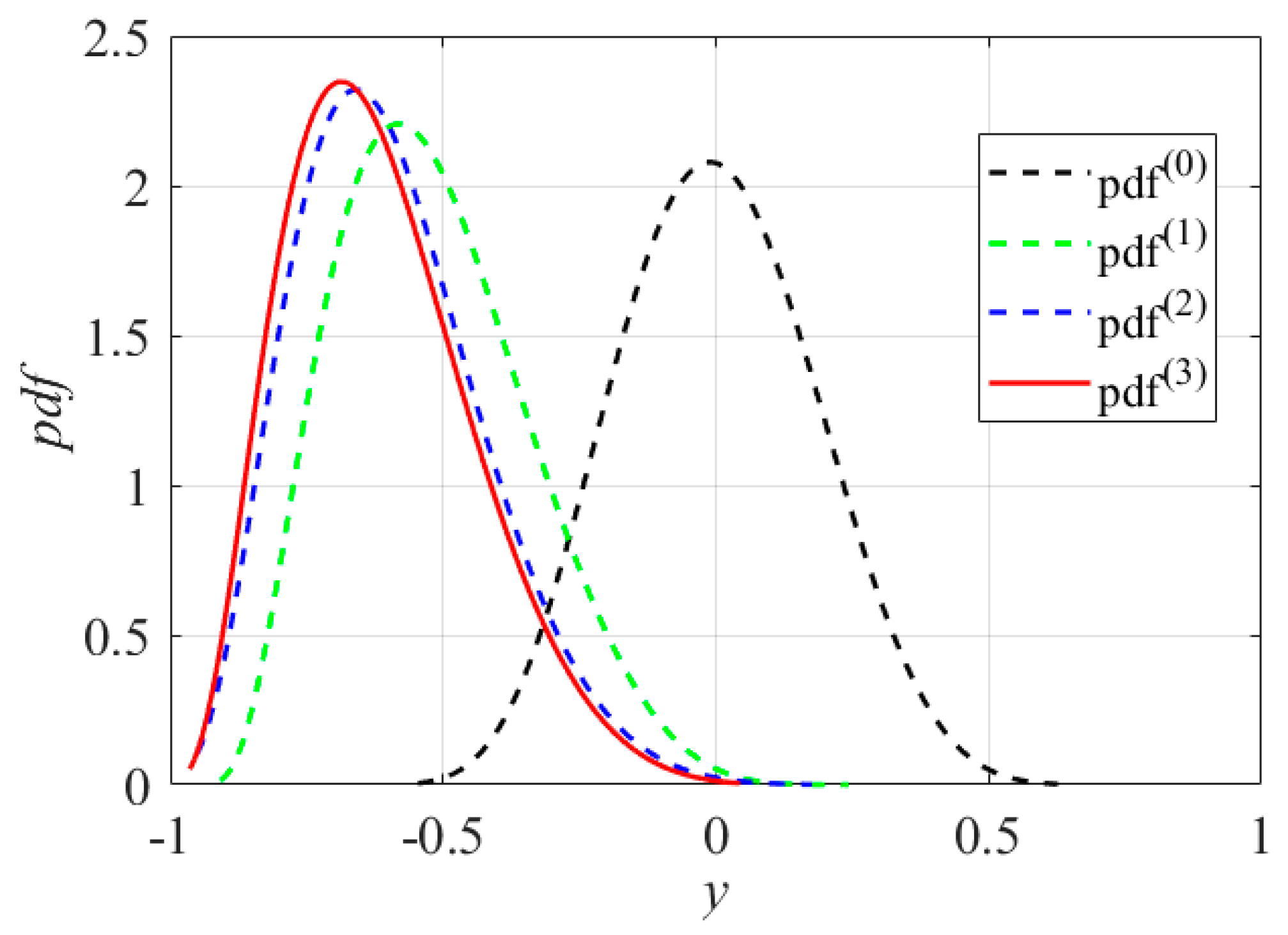
The convergence process of the PDF, , of the inequality function response, , in the probability constraint is illustrated in Figure 5, which shows that moves to in the direction of enhancing reliability in the iterations. Combined with Table 1, it can be found that in , while in . Comparison of and reveals significant variations with respect to the mean values and dispersion degrees, while the locations of the mean values and degrees of dispersion in and show less variation. The convergence process of further validates the reasonability and feasibility of the assumptions in Section 3.3.2 and also demonstrates the accuracy of the optimal RB-DOP solution.
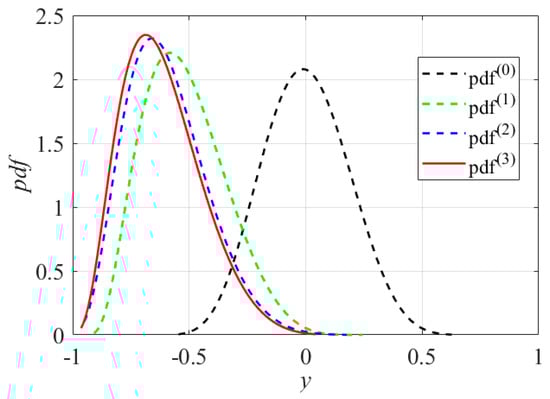
Figure 5.
The convergence process of the PDF, .
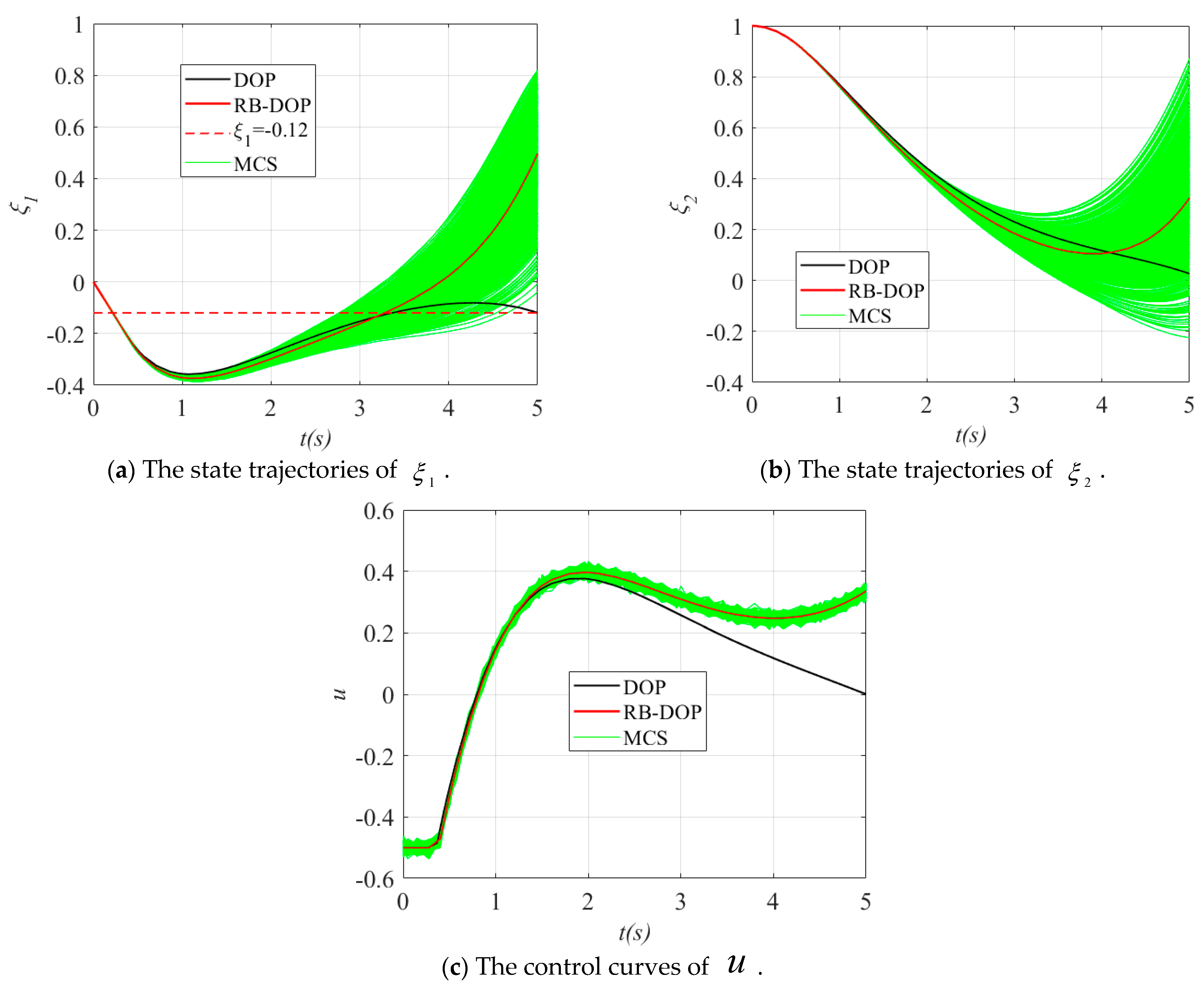
Finally, the state trajectories and control curves in the optimal solutions of DOP and RB-DOP in this example are shown in Figure 6, where the solid black lines indicate the state trajectories or control curves in the optimal DOP solution and the solid red lines represent the state trajectories or control curves in the optimal RB-DOP solution. At the same time, to visualize the effects of the randomness of the control variables on the state trajectories, 1000 control samples were used to create the Monte Carlo simulation (MCS) plots, as shown by the solid green lines. In this example, the control samples follow the normal distribution at all time nodes, where is the optimal control curve in the optimal RB-DOP solution. From the MCS plots in Figure 6, it can be found that although randomness causes small fluctuations in the control variable at each time node (in Figure 6c), these fluctuations have a significant impact on the state trajectories through the state equations as time evolves (in Figure 6a,b). More importantly, almost no trajectories violate the inequality constraint when in Figure 6a, which intuitively proves that the optimal RB-DOP solution obtained by the proposed method satisfies the probability constraint .

Figure 6.
The state trajectories and control curves in the DOP and RB-DOP optimal solutions.
4.2. Numerical Example 2
The RB-DOP in numerical example 2 was adapted from the DOP in the literature [14], which contains three state variables, , and one control variable, . The formulation of this RB-DOP is given as follows:
where it is assumed that follows the normal distribution at every time node and and denote the mean values of and . In this example, the target reliability of the probability constraints was .
The proposed CFRSS-based RB-DOP optimization method was adopted to solve this example, and the iteration results are listed in Table 2. At first, the optimal solution of the deterministic DOP was set as the initial-guess RB-DOP solution . Then, considering the randomness of the control variable, , at , the PDFs and of the inequality function values and were fitted by the Monte Carlo method and the Johnson distribution. And the reliabilities and of the probability constraints, , were 5.37% and 28.35%, calculated from and , respectively.
Table 2.
The iteration results of numerical example 2.
Subsequently, the proposed method solved this example with four iterations. In the first iteration, the shift scalars and were set as 0.2075 and 0.4044 after analyzing and . According to Equation (13), RB-DOP was transformed into a deterministic DOP to be addressed based on and , and the current optimal solution in the first iteration was solved. Then, the PDFs and for and were fitted using the Monte Carlo method and the Johnson distribution, the reliabilities and of the probability constraints in the current design were 98.80% and 99.73%, and the shift scalars and provided to the second iteration were 0.2570 and 0.4621. Similarly, the reliabilities and in the current design in the second iteration were 99.87% and 99.89%, and the shift scalars and provided to the third iteration were 0.2633 and 0.4727. In the third iteration, the -type Johnson distribution was identified to describe the distribution characteristics of , and the PDF of is expressed in Equation (35). Then, the reliabilities and in the current design were 99.89% and 99.90%, and the shift scalars and provided to the fourth iteration were 0.2645 and 0.4727. Since and , the probability constraint, , was satisfied, and only had to be analyzed in the subsequent iterations. In the fourth iteration, the -type Johnson distribution was identified to describe the distribution characteristics of , and the PDF of is expressed in Equation (36). Then, the reliability in the current design was 99.90%, and the shift scalar for the fifth iteration was 0.2645. Obviously, and , such that the probability constraint was also satisfied, and the solving procedure was terminated. Up to this point, the CFRSS-based RB-DOP solving method obtained the optimal solution after four iterations; the optimal objective function value was 0.8806 in RB-DOP, which is 7.85% higher than the counterpart in DOP. This is because the reliability constraints are required to be met in the RB-DOP and are more stringent than the constraints in the corresponding DOP.
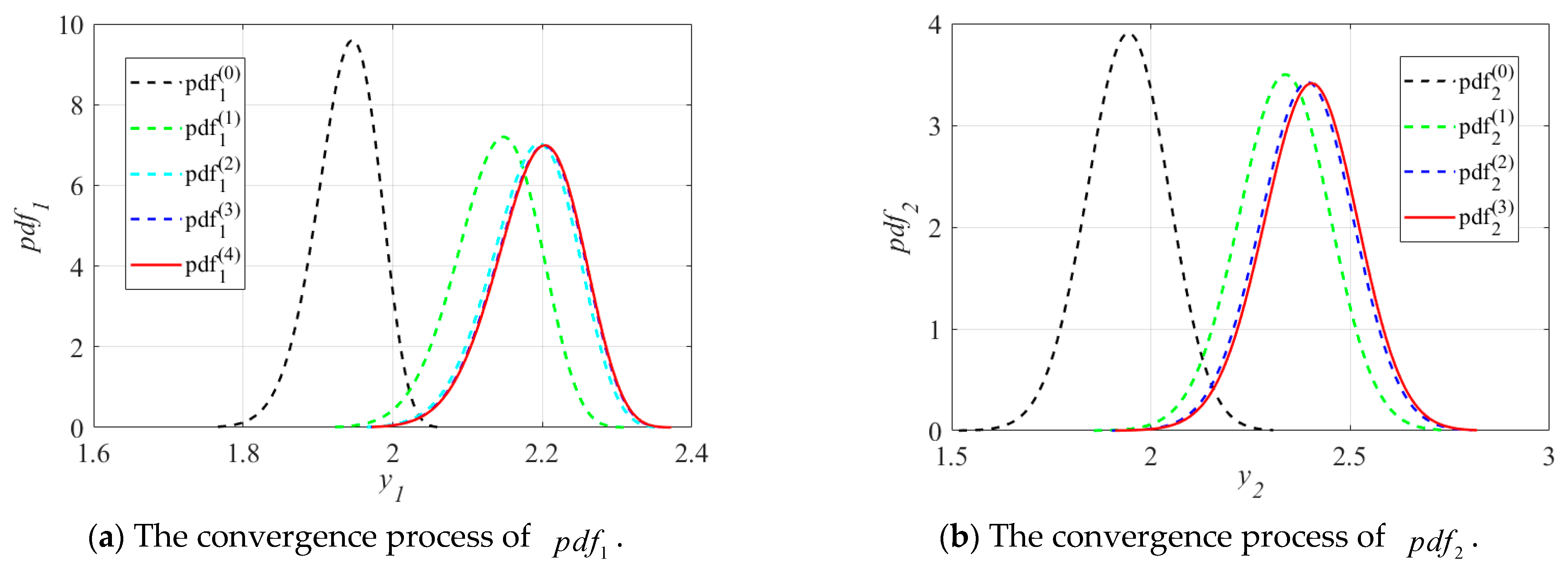
The convergence processes of the PDFs and of the inequality function responses and are illustrated in Figure 7. It can be observed from Figure 7 that and move to and in the direction of enhancing reliability in the iterations. As compared to , changes more significantly not only in the mean values but also in the dispersion degrees, while from to the locations of the mean value and degrees of dispersion show less variation. The variation trend of is consistent with that of . The convergence processes of and further validate the reasonability and feasibility of the assumptions in Section 3.3.2 and also demonstrate the accuracy of the optimal RB-DOP solution.
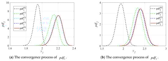
Figure 7.
The convergence processes of PDFs and .
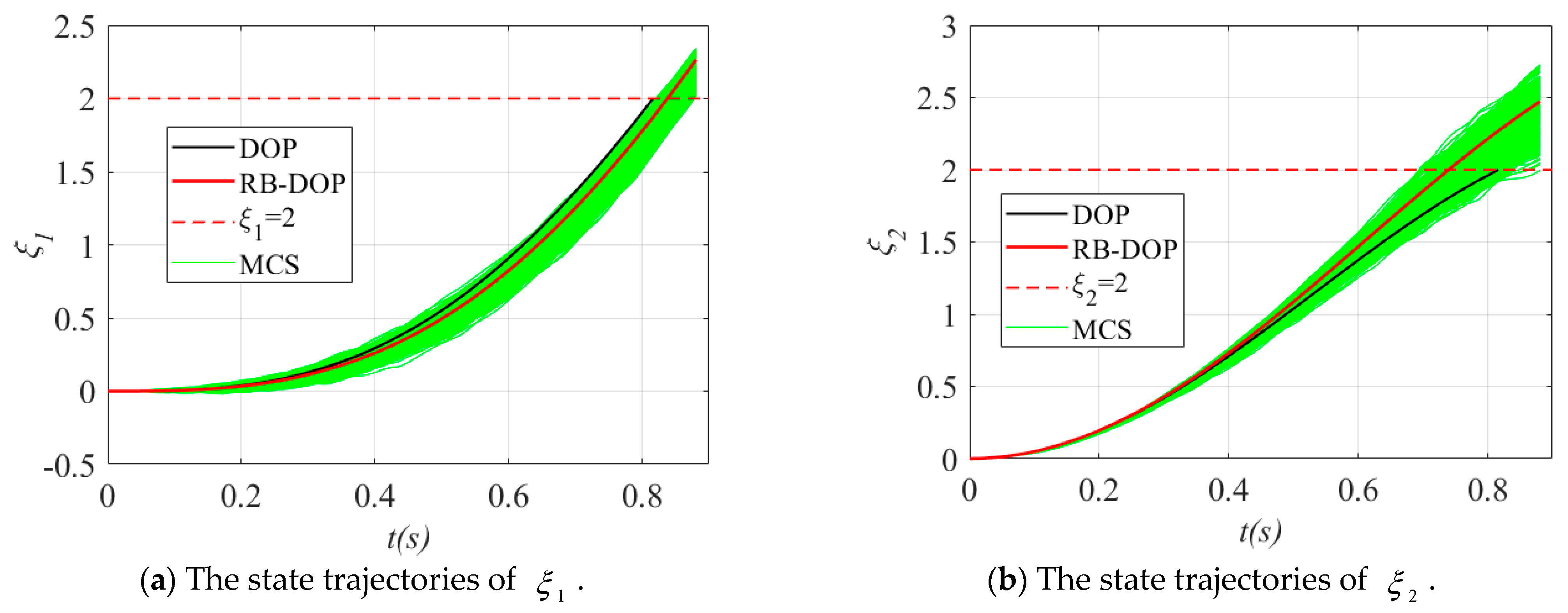
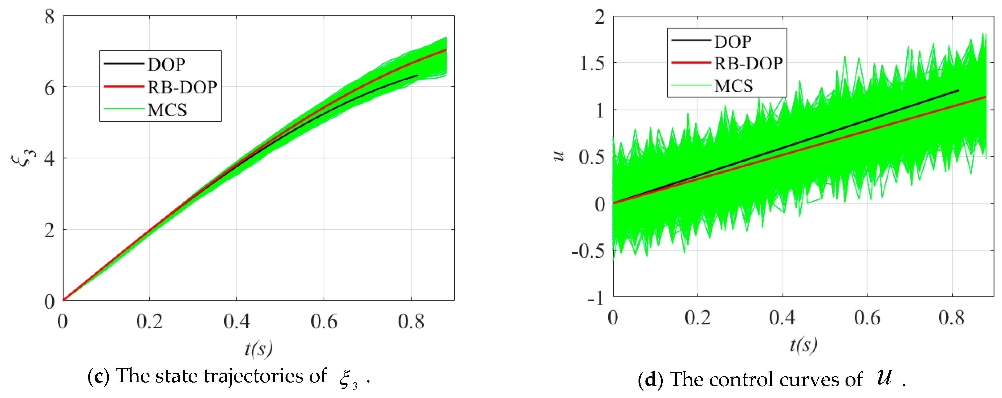
Finally, the state trajectories and control curves in the optimal DOP and RB-DOP solutions in this example are shown in Figure 8, where the solid black lines and solid red lines indicate the optimal DOP and RB-DOP solutions, respectively. Meanwhile, 1000 control samples were used to create the MCS plots, as shown by the solid green lines, to intuitively demonstrate the effects of the randomness of the control variables on the state trajectories. In this example, those control samples follow the normal distribution at all time nodes, where is the optimal control curve in RB-DOP. It can be found from Figure 8d that randomness causes large fluctuations in the control variable at each time node and influences the evolution of state trajectories through the state equations (in Figure 8a–c). What is more important, almost no trajectories violate the inequality constraints in Figure 8a and in Figure 8b when , which intuitively proves that the optimal solution obtained by the CFRSS-based RB-DOP optimization method satisfies the probability constraint.
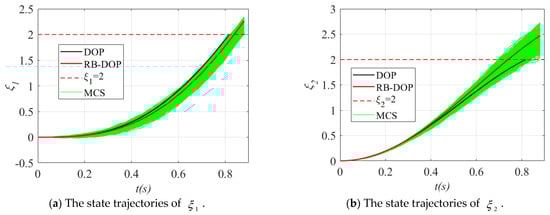
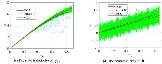
Figure 8.
The state trajectories and control curves in the optimal solution.
4.3. An RB-DOP in Low-Thrust Orbit Transfer
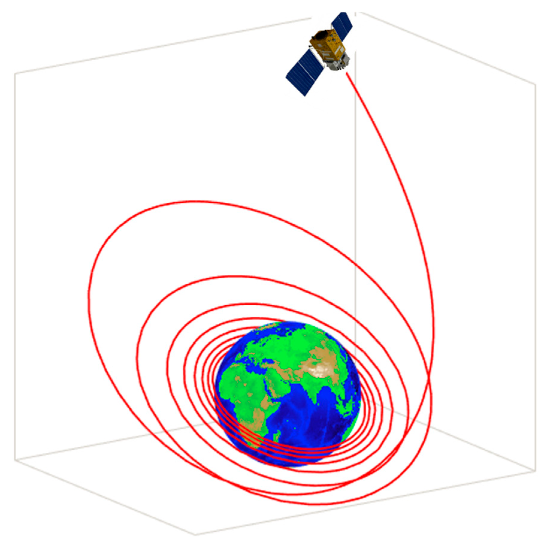
The trajectory optimization of spacecraft transfer from low earth orbit to mission orbit, as shown in Figure 9, is a challenging class of DOP problems, since the dynamics are very nonlinear and the durations of the trajectories are very long [41]. Typically, the goal is to construct the optimal trajectory during the transfer such that the final weight is maximized (i.e., the minimum of fuel is consumed). The DOP of the low-thrust orbit transfer can be represented as
where the state variable involves , , , , , , , and ; is the vector of the control variables; is the fuel weight; denotes the weight of the fuel consumed per unit time; is the specific impulse; and is the thrust.
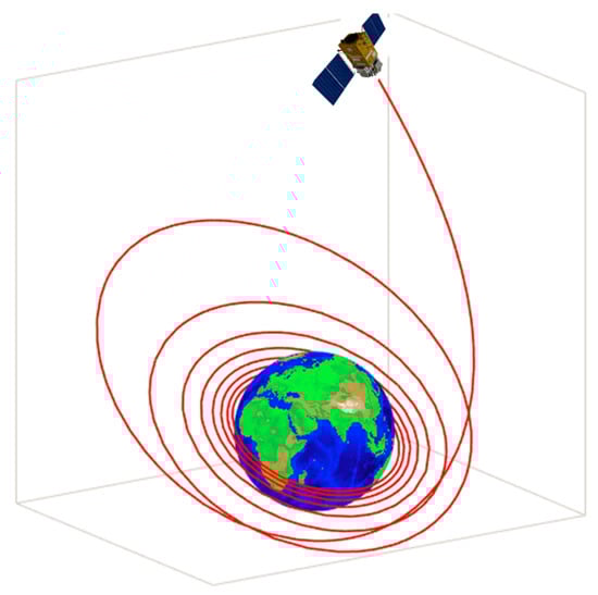
Figure 9.
Schematic diagram of low-thrust orbit transfer.
The matrix is defined by
and the vector
where
The disturbing acceleration vector is defined by
where is the gravitational disturbing acceleration and is the thrust acceleration. More specific details of the model and the values of all the constants in this problem can be found in Ref. [41].
Due to the inherent properties of the controller, the control variables, , have random errors at every time node. Therefore, the control variables, , can be treated as random variables. To analyze the influence of the random control variables, , on a spacecraft low-thrust orbit transfer mission, this work defines the control variables, , as following the normal distribution at each time node . Meanwhile, the DOP is transformed into RB-DOP by converting some of the equality constraints and inequality constraints in the deterministic DOP into probability constraints, as shown below:
The CFRSS-based RB-DOP optimization method was used to optimize this RB-DOP, and the optimal solution converged with three iterations; the iteration results are shown in Table 3. In the initial iteration, the optimal solution of the deterministic DOP was set as the initial-guess RB-DOP solution . The reliabilities and of the probability constraints in the initial design were 47.42% and 100.00%, according to and , fitted by the Monte Carlo method and the Johnson distribution. Clearly, the probability constraint, , was satisfied in the initial iteration, and the shift scalar, , for the subsequent iterations was 0. After three iterations, the CFRSS-based RB-DOP optimization method acquired the optimal solution, the -type Johnson distribution was identified to describe the distribution characteristics of in the current design , and the PDF of is expressed in Equation (43). Moreover, the reliability, , in the third iteration was 99.90%, calculated by , and the final weight of the fuel was 0.09575 kg.
Table 3.
The iteration results for this engineering example.
In the meantime, the convergence process of the PDF of is illustrated in Figure 10. It can be observed from Figure 10 that moved to in the direction of enhancing reliability in the three iterations; the improvements from to in terms of the mean values and the dispersion degrees are quite distinct, while the mean value and the dispersion degree of converged from to by fine-tuning in the second and third iterations. The convergence process of further validates the reasonability and feasibility of the assumptions in Section 3.3.2 and also demonstrates the accuracy of the RB-DOP optimal solution.
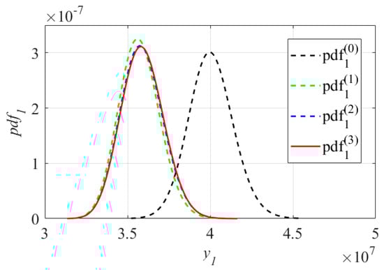
Figure 10.
The convergence process of the PDF .
With the optimal solution of DOP as the benchmark, the comparison results of the optimal DOP and RB-DOP solutions are listed in Table 4. As can be seen from Table 4, the fuel consumed by the spacecraft in RB-DOP is 0.35775 kg, which is slightly more than the 0.35762 kg consumed in DOP. The terminal state of the state component in RB-DOP is 10,907,302.9 m, which is 10.42% lower than the 12,176,760 m in DOP. In turn, the optimal trajectory in RB-DOP improves the reliability of the spacecraft system by 52.48%, from 47.42% to 99.90%, for the probability constraint.
Table 4.
Comparison of optimal DOP and RB-DOP solutions in low-thrust orbit transfer.
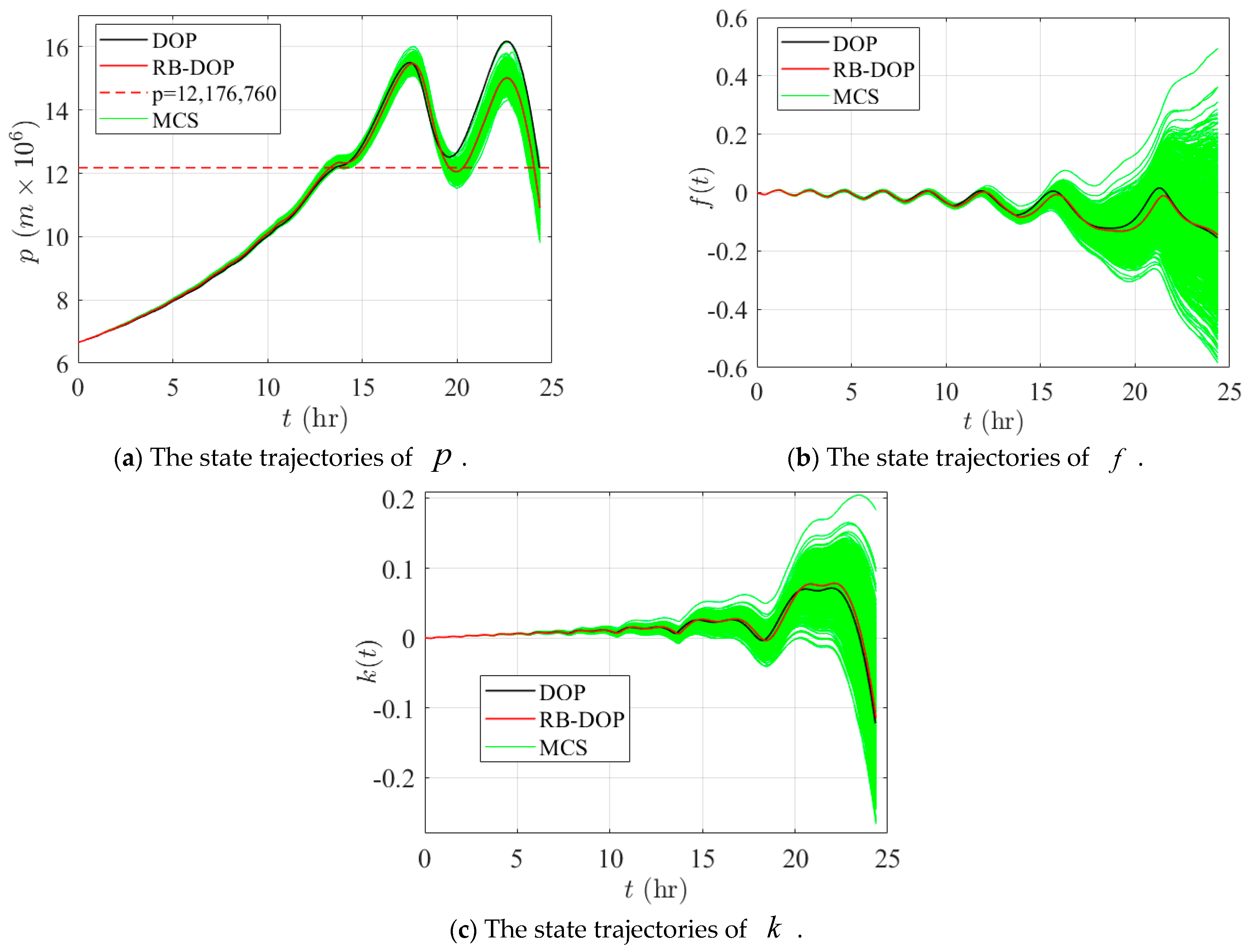
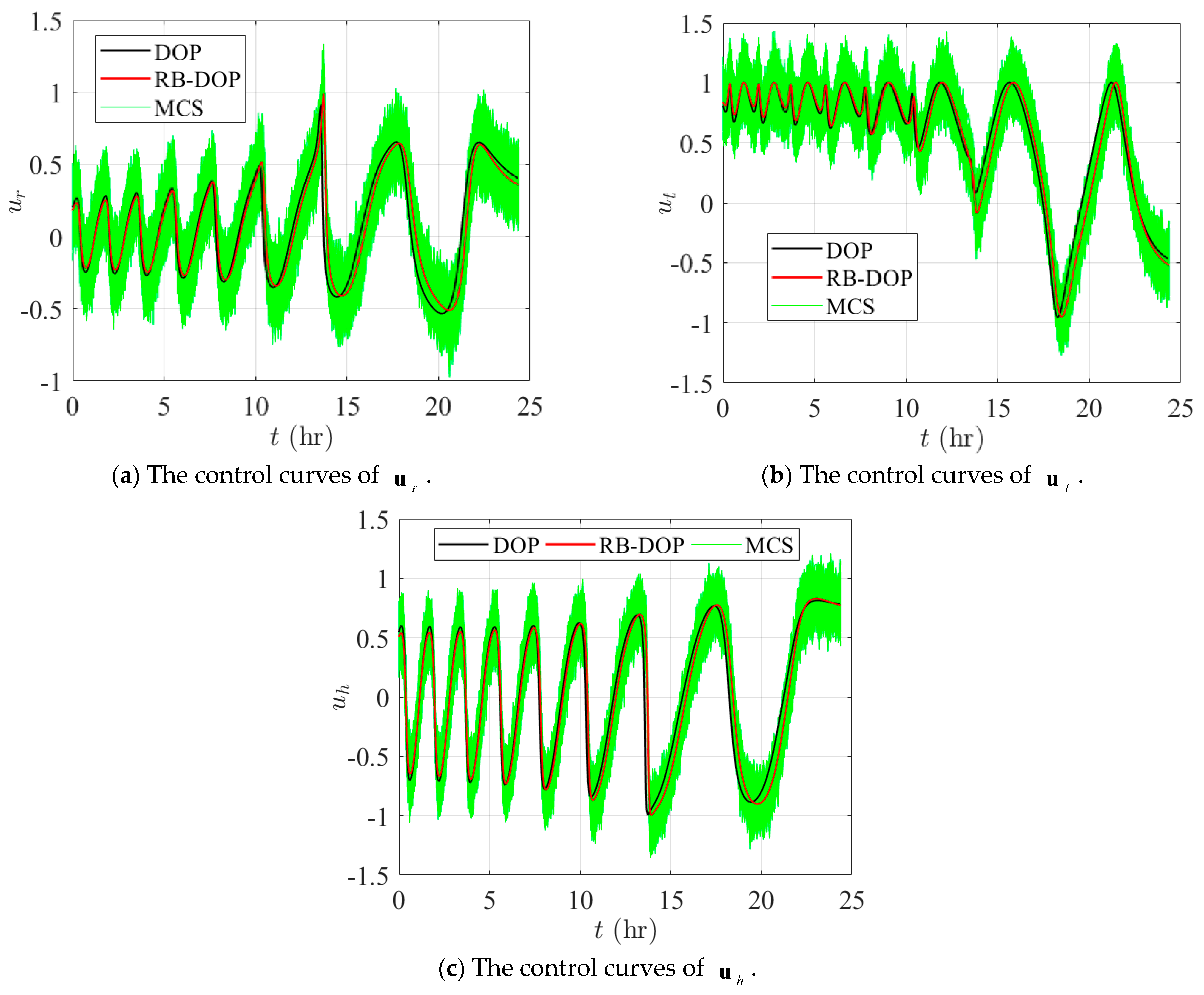
Finally, Figure 11 and Figure 12 demonstrate the state trajectories and control curves in the optimal DOP and RB-DOP solutions by the black and solid red lines. Meanwhile, to intuitively demonstrate the effects of the randomness of the control variables on the state trajectories, 1000 control samples, i.e., the solid green lines, were used to create the MCS plots. And those control samples followed the normal distribution at all time nodes, where represents the optimal control curves in RB-DOP. It can be observed from Figure 11 that randomness causes fluctuations in the control variable at each time node and influences the evolution of the state trajectories through the state equation (in Figure 12). Since spacecraft use a small thrust for orbit transfer, the transfer time is long; the spacecraft took about 24.33 h to complete the orbit transfer mission in RB-DOP and DOP. Therefore, changes in the control variables, , caused by the randomness have a significant effect on the state variables, , especially the state component, . Moreover, almost no trajectories violate the inequality constraint in Figure 11a at the terminal time node, which intuitively proves that the optimal solution obtained by the CFRSS-based RB-DOP optimization method satisfied the probability constraint.
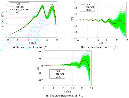
Figure 11.
State trajectories in DOP and RB-DOP optimal solutions.
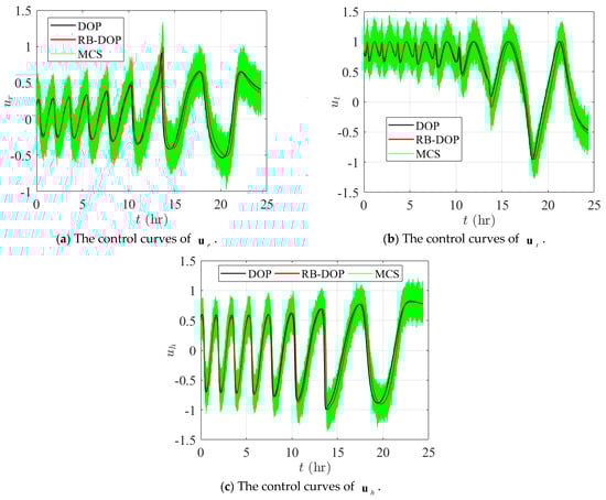
Figure 12.
Control curves for DOP and RB-DOP optimal solutions.
5. Conclusions
To eliminate the adverse impact of random control variables on dynamic system performance and satisfy the higher requirement of dynamic system reliability, this work introduces the reliability-based dynamic optimization problem (RB-DOP) and defines RB-DOP by assigning randomness to control variables at all time grid nodes. Then, the concept of the constraint function response shift scalar (CFRSS) is presented based on SORA, and the CFRSS-based RB-DOP optimization method is proposed for solving RB-DOP effectively and efficiently. The proposed method decouples the nested RB-DOP into an equivalent deterministic DOP and a CFRSS search problem, and the DOP and the CFRSS search problem are addressed iteratively until the optimal solution to RB-DOP converges. Finally, two numerical examples and a low-thrust orbit transfer problem are investigated to illustrate that the optimal control law generated by the proposed method can dramatically improve the reliability of the dynamic system.
With regard to the future research focus, one question is how to acquire PDFs quickly by efficient numerical methods other than the Monte Carlo method and the Johnson distribution. Furthermore, the control law solved in the RB-DOP may fail when the actual variance of randomness is larger than the set value. Therefore, research into the control law considering the form of state feedback in RB-DOP may be another future direction.
Author Contributions
Data curation, Y.W.; Formal analysis, Y.W.; Funding acquisition, P.Q.; Methodology, Q.Z.; Resources, Q.Z.; Software, P.Q.; Supervision, Q.Z.; Validation, Q.Z.; Visualization, Y.W.; Writing—original draft, P.Q.; Writing—review and editing, P.Q. All authors have read and agreed to the published version of the manuscript.
Funding
This work was supported by the National Natural Science Foundation of China (Grant No. 52405286). This support is gratefully acknowledged.
Data Availability Statement
Researchers interested in this method can access the code through the corresponding author.
Conflicts of Interest
The authors declare that they have no known competing financial interests or personal relationships that could have appeared to influence the work reported in this paper.
Nomenclature
| Mean state variables | Constraint function response shift scalar of | ||
| Mean control variables | Reduced form of | ||
| Objective function of the DOP and RB-DOP | Shift vector component of state and control design variables in the kth iteration | ||
| Objective function of the RBDO | Discrete matrices of | ||
| The ith inequality constraint function | Response value of the constraint | ||
| Discrete state matrix | The PDF of | ||
| Discrete control matrix | The PDF of for design variables | ||
| Random design variables | The PDF of for design variables in the kth iteration | ||
| Mean values of | Constraint function response at point | ||
| Actual reliability of | Target reliability of | ||
| Standard normal cumulative distribution function | Constraint function response shift distance | ||
| Target reliability index of | Integral term of the PDF moves | ||
| Shift vector in the kth iteration | Inverse function of | ||
| The minimum performance target point in the original space | Control sample set | ||
| Standard normal variables converted from | The normal distribution with mean values and standard deviation | ||
| Mean values of | State trajectory sample set | ||
| Mean values of | Constraint function response set | ||
| The ith probability constraint enforced on the design variables at the time node | Error tolerance |
Appendix A
Johnson Distribution
To facilitate the uniform expression of the PDF for various different types of continuous-type random variables, Johnson [43] proposed the four-parameter Johnson distribution. And the PDF of the Johnson distribution is
where parameters and stand for the shape parameters, parameter is the position parameter, and parameter is the scale parameter. is a simple functional expression, and the Johnson distribution can be divided into four types according to , such as unbounded , normal , log-normal , and bounded . The specific expressions for and are shown below:
Moreover, the Johnson transformation equation can transform the continuous random variable, , into a random variable, , that follows the standard normal distribution. The Johnson transformation equation can be expressed as
Due to containing multiple parameters and types, the Johnson distribution can express more distributional characteristics by fitting the data. And the Johnson distribution can approximate any of the standard continuous distribution models by choosing the appropriate type and adjusting the parameters [43]. To accurately estimate the four parameters in the Johnson distribution, DeBrota et al. [44] proposed four methods, including the Moment Matching, Percentile Matching, Least Squares, and Minimum Lp Norm Estimation methods.
References
- Allison, J.T.; Guo, T.; Han, Z. Co-design of an active suspension using simultaneous dynamic optimization. J. Mech. Des. 2014, 136, 081003. [Google Scholar] [CrossRef]
- Qiao, P.; Liu, X.; Zhang, Q.; Xu, B. An optimal control algorithm toward unknown constrained nonlinear systems based on the sequential sampling and updating of surrogate model. ISA Trans. 2024, 153, 117–132. [Google Scholar] [CrossRef]
- Zhang, Q.; Wu, Y.; Qiao, P.; Lu, L.; Xia, Z. A right-hand side function surrogate model-based method for the black-box dynamic optimization problem. J. Mech. Des. 2023, 145, 091701. [Google Scholar] [CrossRef]
- Pontryagin, L.S.; Boltyanskii, V.; Gamdrelidze, R.; Mishchenko, E. Mathematical Theory of Optimal Processes, 1st ed.; Interscience: New York, NY, USA, 1962. [Google Scholar]
- Bellman, R. Dynamic Programming; Princeton University Press: Princeton, NJ, USA, 1957. [Google Scholar]
- Liu, P.; Li, G.; Liu, X.; Xiao, L.; Wang, Y.; Yang, C.; Gui, W. A novel non-uniform control vector parameterization approach with time grid refinement for flight level tracking optimal control problems. ISA Trans. 2018, 73, 66–78. [Google Scholar] [CrossRef] [PubMed]
- Tang, X.; Xu, H. Multiple-interval pseudospectral approximation for nonlinear optimal control problems with time-varying delays. Appl. Math. Model. 2019, 68, 137–151. [Google Scholar] [CrossRef]
- Delkhosh, M.; Cheraghian, H. An efficient hybrid method to solve nonlinear differential equations in applied sciences. Comput. Appl. Math. 2022, 41, 322. [Google Scholar] [CrossRef]
- Pirastehzad, A.; Yazdanpanah, M.J. A Successive Pseudospectral-Based Approximation of the Solution of Regulator Equations. IEEE Trans. Autom. Control 2022, 67, 1760–1775. [Google Scholar] [CrossRef]
- Song, Y.; Pan, B.; Fan, Q.; Xu, B. A computationally efficient sequential convex programming using Chebyshev collocation method. Aerosp. Sci. Technol. 2023, 141, 108584. [Google Scholar] [CrossRef]
- Deshmukh, A.P.; Allison, J.T. Multidisciplinary dynamic optimization of horizontal axis wind turbine design. Struct. Multidiscip. Optim. 2016, 53, 15–27. [Google Scholar] [CrossRef]
- Herber, D.R.; Allison, J.T. Nested and simultaneous solution strategies for general combined plant and control design problems. J. Mech. Des. 2019, 141, 011402. [Google Scholar] [CrossRef]
- Zhang, Q.; Wu, Y.; Qiao, P. A Dendrite Net based decoupled framework for the reliability-based control co-design problem. Qual. Reliab. Eng. Int. 2024, 40, 925–947. [Google Scholar] [CrossRef]
- Biegler, L.T.; Zavala, V.M. Large-scale nonlinear programming using IPOPT: An integrating framework for enterprise-wide dynamic optimization. Comput. Chem. Eng. 2009, 33, 575–582. [Google Scholar] [CrossRef]
- Serrancolí, G.; Pàmies-Vilà, R. Analysis of the influence of coordinate and dynamic formulations on solving biomechanical optimal control problems. Mech. Mach. Theory 2019, 142, 103578. [Google Scholar] [CrossRef]
- Schueller, G.I.; Jensen, H.A. Computational methods in optimization considering uncertainties—An overview. Comput. Methods Appl. Mech. Eng. 2008, 198, 2–13. [Google Scholar] [CrossRef]
- Meng, Z.; Zhang, Z.; Zhou, H. A novel experimental data-driven exponential convex model for reliability assessment with uncertain-but-bounded parameters. Appl. Math. Model. 2020, 77, 773–787. [Google Scholar] [CrossRef]
- Bey, O.; Chemachema, M. Finite-time event-triggered output-feedback adaptive decentralized echo-state network fault-tolerant control for interconnected pure-feedback nonlinear systems with input saturation and external disturbances: A fuzzy control-error approach. Inf. Sci. 2024, 669, 120557. [Google Scholar] [CrossRef]
- Bounemeur, A.; Chemachema, M. Finite-time output-feedback fault tolerant adaptive fuzzy control framework for a class of MIMO saturated nonlinear systems. Int. J. Syst. Sci. 2024, 56, 733–752. [Google Scholar] [CrossRef]
- Meng, Z.; Yildiz, B.S.; Li, G.; Zhong, C.T.; Mirjalili, S.; Yildiz, A.R. Application of state-of-the-art multiobjective metaheuristic algorithms in reliability-based design optimization: A comparative study. Struct. Multidiscip. Optim. 2023, 66, 191. [Google Scholar] [CrossRef]
- Shirgir, S.; Shamsaddinlou, A.; Zare, R.N.; Zehtabiyan, S.; Bonab, M.H. An efficient double-loop reliability-based optimization with metaheuristic algorithms to design soil nail walls under uncertain condition. Reliab. Eng. Syst. Saf. 2023, 232, 109077. [Google Scholar] [CrossRef]
- Ma, Y.-Z.; Jin, X.-X.; Wu, X.-L.; Xu, C.; Li, H.-S.; Zhao, Z.-Z. Reliability-based design optimization using adaptive Kriging-A single-loop strategy and a double-loop one. Reliab. Eng. Syst. Saf. 2023, 237, 109386. [Google Scholar] [CrossRef]
- Kohtz, S.; Zhao, J.; Renteria, A.; Lalwani, A.; Xu, Y.; Zhang, X.; Haran, K.S.; Senesky, D.; Wang, P. Optimal sensor placement for permanent magnet synchronous motor condition monitoring using a digital twin-assisted fault diagnosis approach. Reliab. Eng. Syst. Saf. 2024, 242, 109714. [Google Scholar] [CrossRef]
- Zhang, J.; Gao, L.; Xiao, M.; Lee, S.; Eshghi, A.T. An active learning Kriging-assisted method for reliability-based design optimization under distributional probability-box model. Struct. Multidiscip. Optim. 2020, 62, 2341–2356. [Google Scholar] [CrossRef]
- Xiao, M.; Zhang, J.; Gao, L. A system active learning Kriging method for system reliability-based design optimization with a multiple response model. Reliab. Eng. Syst. Saf. 2020, 199, 106935. [Google Scholar] [CrossRef]
- Meng, Z.; Guo, L.; Wang, X. A general fidelity transformation framework for reliability-based design optimization with arbitrary precision. Struct. Multidiscip. Optim. 2022, 65, 14. [Google Scholar] [CrossRef]
- Zhang, J.; Xiao, M.; Gao, L.; Fu, J. A novel projection outline based active learning method and its combination with Kriging metamodel for hybrid reliability analysis with random and interval variables. Comput. Methods Appl. Mech. Eng. 2018, 341, 32–52. [Google Scholar] [CrossRef]
- Zhu, X.; Lu, Z.; Yun, W. An efficient method for estimating failure probability of the structure with multiple implicit failure domains by combining Meta-IS with IS-AK. Reliab. Eng. Syst. Saf. 2020, 193, 106644. [Google Scholar] [CrossRef]
- Jiang, C.; Qiu, H.; Gao, L.; Wang, D.; Yang, Z.; Chen, L. EEK-SYS: System reliability analysis through estimation error-guided adaptive Kriging approximation of multiple limit state surfaces. Reliab. Eng. Syst. Saf. 2020, 198, 106906. [Google Scholar] [CrossRef]
- Nikolaidis, E.; Burdisso, R. Reliability based optimization: A safety index approach. Comput. Struct. 1988, 28, 781–788. [Google Scholar] [CrossRef]
- Fang, Y.; He, C.; Su, Y.; Feng, K.; He, Z. Supplement to the reliability index approach and its application to tunnel reliability problems. Comput. Geotech. 2023, 163, 105767. [Google Scholar] [CrossRef]
- Tu, J.; Choi, K.K.; Park, Y.H. A new study on reliability-based design optimization. J. Mech. Des. 1999, 121, 557–564. [Google Scholar] [CrossRef]
- Du, X.P.; Chen, W. Sequential optimization and reliability assessment method for efficient probabilistic design. J. Mech. Des. 2004, 126, 225–233. [Google Scholar] [CrossRef]
- Li, G.; Yang, H.; Zhao, G. A new efficient decoupled reliability-based design optimization method with quantiles. Struct. Multidiscip. Optim. 2020, 61, 635–647. [Google Scholar] [CrossRef]
- Liu, W.-S.; Cheung, S.H. Reliability based design optimization with approximate failure probability function in partitioned design space. Reliab. Eng. Syst. Saf. 2017, 167, 602–611. [Google Scholar] [CrossRef]
- Zhang, J.; Xiao, M.; Gao, L. A new local update-based method for reliability-based design optimization. Eng. Comput. 2021, 37, 3591–3603. [Google Scholar] [CrossRef]
- Rocchetta, R.; Crespo, L.G. A scenario optimization approach to reliability-based and risk-based design: Soft-constrained modulation of failure probability bounds. Reliab. Eng. Syst. Saf. 2021, 216, 107900. [Google Scholar] [CrossRef]
- Jiang, X.; Lu, Z. A novel quantile-based sequential optimization and reliability assessment method for safety life analysis. Reliab. Eng. Syst. Saf. 2024, 243, 109810. [Google Scholar] [CrossRef]
- Zhang, Z.; Deng, W.; Jiang, C. A PDF-based performance shift approach for reliability-based design optimization. Comput. Methods Appl. Mech. Eng. 2021, 374, 113610. [Google Scholar] [CrossRef]
- Allison, J.T.; Herber, D.R. Multidisciplinary design optimization of dynamic engineering systems. AIAA J. 2014, 52, 691–710. [Google Scholar] [CrossRef]
- Betts, J.T. Practical Methods for Optimal Control and Estimation Using Nonlinear Programming, 3rd ed.; Society for Industrial and Applied Mathematics: Philadelphia, PA, USA, 2010. [Google Scholar]
- Zhang, Q.; Wu, Y.; Lu, L.; Qiao, P. A single-loop framework for the reliability-based control co-design problem in the dynamic system. Machines 2023, 11, 262. [Google Scholar] [CrossRef]
- Johnson, N.L. Systems of frequency curves generated by methods of translation. Biometrika 1949, 36, 149–176. [Google Scholar] [CrossRef]
- Debrota, D.J.; Roberts, S.D.; Swain, J.J.; Dittus, R.S.; Wilson, J.R.; Venkatraman, S. Input modeling with the Johnson System of distributions. In Proceedings of the 1988 Winter Simulation Conference Proceedings, San Diego, CA, USA, 12–14 December 1988; pp. 165–179. [Google Scholar]


Disclaimer/Publisher’s Note: The statements, opinions and data contained in all publications are solely those of the individual author(s) and contributor(s) and not of MDPI and/or the editor(s). MDPI and/or the editor(s) disclaim responsibility for any injury to people or property resulting from any ideas, methods, instructions or products referred to in the content. |
© 2025 by the authors. Licensee MDPI, Basel, Switzerland. This article is an open access article distributed under the terms and conditions of the Creative Commons Attribution (CC BY) license (https://creativecommons.org/licenses/by/4.0/).