Verification of Detectability for Time Labeled Petri Net Systems with Unobservable Transitions

Abstract

We investigate the detectability verification problem of time-dependent systems modeled by time labeled Petri nets that are a typical time-dependent model of many computer-integrated systems in modern society, characterized by networked connections. In a time labeled Petri net, the detectability proposed in this paper characterizes the current state of a time-dependent system that can be uniquely determined after a finite number of observations within a given time instant. Moreover, we further define strong and weak detectability in a time labeled Petri net system. To verify strong and weak detectability, we excogitate a label-based state class graph, which is not required to enumerate all states of a system, to compute the states for a given real-time observation. Based on the proposed label-based state class graph, an information structure called a timed state observer is formulated to verify strong and weak detectability. The proposed verification technique is advantageous and is effectively applied to an intelligent garage system, since the enumeration of all states of the time-dependent system is not required.

1. Introduction

In cyber-physical systems, the system dynamic is generally incompletely known thanks to restrictions of deployed sensors or environmental constraints, such as these systems usually being partially observed, i.e., only a part of system behavior can be observed by an external observer. In this case, system states are only estimated by observational system outputs. In a lot of realistic applications exhibiting the features of discrete-event systems (DESs), system security or the safety of information flows is usually of paramount importance. Recent years have witnessed many interesting research results on these information-related properties in the domain of discrete-event systems, such as detectability detection [1], fault diagnosis and diagnosability analysis [2], opacity verification [3,4,5], and the design of supervisory controllers [6], which rely on the state estimation of partially observable systems.

Deciding on precise system states is critical for many problems of system analysis and synthesis of discrete-event systems since various system control requirements can be equivalently transformed into state detection problems. The classical theory of observers in continuous-time dynamical systems is concerned with the reconstruction of system state space from the input and output of a system. A conceptually appealing and generally useful property of a continuous-time dynamical system is the detectability that is generalized from the observer theory [7].

The notion of detectability was originally formulated in the framework of deterministic finite automata in [8] for discrete-event systems. Technically, detectability is a system property, implying that, given a current observation (an observational system output), the current and the subsequent states can be uniquely inferred within a finite number of observational steps, i.e., after a finite number of labels is generated by the system. Moreover, four types of detectability are proposed: strong detectability, weak detectability, strong periodic detectability, and weak periodic detectability. Moreover, the techniques for verifying these four types of detectability were developed. These notions are different but correlated. For example, strong detectability refers to the determinism of a unique current and subsequent system states for all possible trajectories decided by an observation, while weak detectability implies the determinism of a unique current and subsequent system states for certain possible trajectories decided by an observation. The sufficient and necessary conditions for both properties can be derived from the observer of a system model. Further, in [9], the authors expand detectability to non-deterministic finite automata and develop a detector to verify strong detectability.

Petri nets are a prevailing yet powerful vehicle for the modeling and control of discrete-event systems and have improved modeling capability over finite automata. For example, strong and weak detectability are proposed in labeled Petri nets (LPNs) [10], and computational complexity analysis for verifying different versions of detectability is accordingly reported [11,12]. In a bounded LPN, addressing the detectability problem generally requires the construction of a reachability graph (RG), which is a finite automaton. Based on an RG, its RG observer is further developed for state estimation. It is well known that the complexity of constructing an RG for an LPN system is exponential to the size of this LPN system. To address this problem, a basis reachability graph-based method for verifying detectability with no necessity to enumerate all the states of a system is reported in [13].

In realistic applications such as healthcare systems [14], smart houses systems [15], and commercial systems [16], the time factor serves a crucial and vital role in both the establishment and investigation of timed models. For the sake of enriching the description of detectability of DESs in this paper, we introduce the time factor to specify the behavior of realistic systems [17,18,19,20,21]. In a time labeled Petri net (TLPN) system, an event is required to occur within a time horizon, which implies that an event is associated with a transition with the time property. Particularly, each transition is constrained to a time horizon and each state is a pair $(M_x,{\mathrm{\Phi }}_x)$, in which $M_x$ is a logical marking and ${\mathrm{\Phi }}_x$ is a family of time-dependent inequalities.

In the TLPN framework, most studies touch on opacity verification [22], state estimation [23], and fault diagnosis [24]. A state class graph aims to abstract the state information of a TLPN, where the nodes are the state classes of a TLPN and the edges are tagged with time constraints of transitions. Constructing a state class graph is an essential step in TLPNs, and an array of results has been documented relying on state class graphs [25,26,27]. A state class graph is designed for the abstraction of the state information of a TLPN, where the nodes are the state classes in a TLPN and each edge is tagged by a time constraint. In [28], the authors develop an approach to checking diagnosability using model-checking techniques and transform the pattern diagnosability problem to examine the linear-time properties of a time Petri net (TPN) system. Basile et al. develop a graph called a modified state class graph (MSCG), where each edge is associated with an event and a time horizon, for addressing the state estimation problem in TLPNs [23]. In contrast to MSCGs, the size of the graph developed in this paper depends on the length of a given sequence of observable labels, and the enumeration of all states is avoided. In addition, a revised state class graph is developed to source the evolution of a timed observation for path detectability verification [29]. Verifying path detectability requires searching all paths associated with all prefixes of the timed observation. Since the method proposed in this paper only needs to solve for the longest path associated with the timed observation, the proposed method in this paper is efficient.

Indeed, as far as we know, few works address the detectability verification problem in timed models. Detectability is a crucial aspect when considering time factors. By verifying detectability, one can ensure that the state of the time-dependent system can be inferred from a timed observation, which is crucial for the robustness and accuracy of the system. Effective state detection is pivotal in many real-world applications, including smart houses, automated cargo assembly, freight transportation, manufacturing, automated driving, rocket and satellite systems, etc. These systems are time-dependent, which means that apart from the basic tasks needing to be accomplished following a prescribed order, the state of a system must also be determined within specific time constraints to ensure safety features. Therefore, we need to abstract and investigate the performances and behaviors of time-dependent systems.

Under the framework of timed automata, Dong et al. propose the notions of strong and delayed detectability and investigate corresponding verification approaches [30]. They show that verifying strong and delayed detectability of timed automata is decidable. In a previous study, we introduced path detectability in TLPNs and the time information overlap problem caused by indistinguishable paths in TLPNs [29]. To overcome this problem, we developed a revised state class graph observer to verify path detectability by checking the event tags of the edges. However, it does not consider strong and weak detectability for a TLPN system. In this paper, we propose strong and weak detectability of a real-time observation (RTO) under the framework of TLPNs. Hence, one is required to estimate the state after the occurrence of each event in an RTO. Then, we develop an approach to verifying the proposed detectability. The main contributions of this paper are described below.

(1) Strong and weak detectability are formally defined in a TLPN system.

(2) An algorithm to construct a label-based state class graph (LSCG) with respect to an RTO is developed. Given an RTO, we only need to compute the states associated with the observable sequence within a given time.

(3) On the basis of the proposed LSCG, a timed state observer, which computes the states reached by each event of an RTO, is developed. By constructing the timed state observer, strong and weak detectability can be verified effectively.

2. Problem Statement

For the economy of space, the preliminaries of Petri nets, TPNs, and TLPNs are referred to [31]. Under the framework of TLPNs, detectability is a property that the current state of a system is uniquely determined after a limited length of observation within a given time. To obtain the main results about the detectability of TLPNs, it is assumed that

(A1) The TLPN system is bounded.

(A2) There is no cycle in the TLPN system that consists only of unobservable transitions.

(A3) The summation of the lower bounds of time intervals associated with the transitions in a cycle of the TLPN exceeds zero.

These three assumptions do not constrain the applicability of the proposed techniques, since most cyber-physical systems are bounded and unobservable cycles are unrealistic to fire in zero time.

2.1. State Estimation

In a TLPN system, the observer could merely acquire the observable labels and their corresponding time instants. An RTO $\mathcal{O}$ of a TLPN is defined as a pair $(\rho ,\tau )$, in which $\rho$ is a time-labeled observation (TLO) and $\tau$ is a time instant. In this work, $\tau$ is the time instant at which the last label is observed in $\rho$. In what follows, we proceed in the context of a TLPN $G=(\mathcal{N},M_0,I,E,\ell )$.

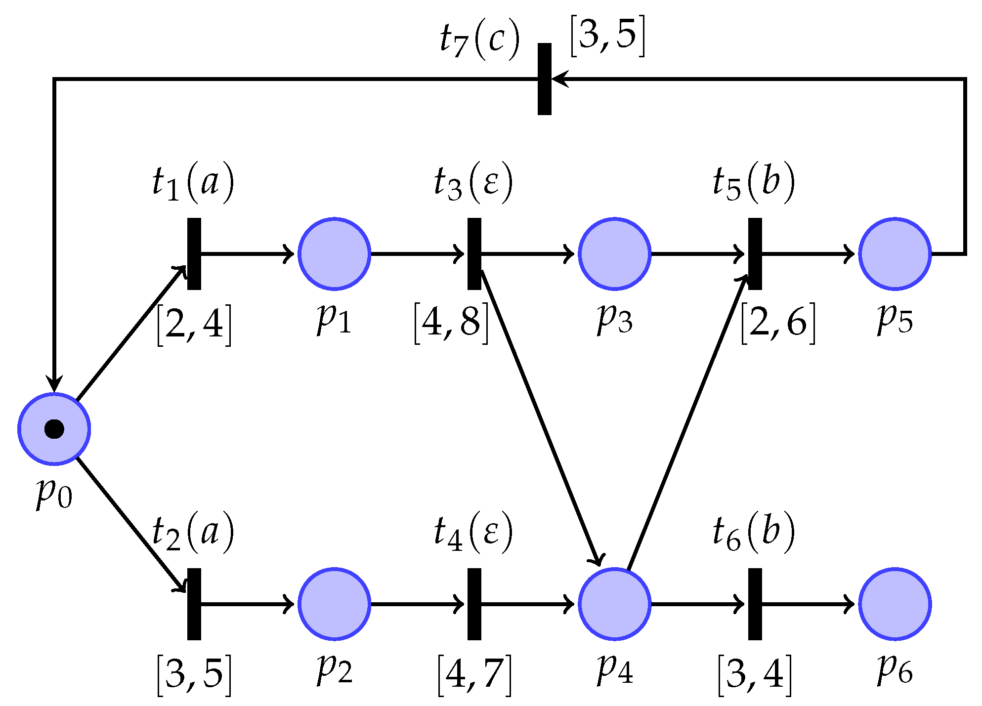
Definition 1.

Let $\mathcal{O}=(\rho ,\tau )$ be an RTO and $(M_0,{\mathrm{\Phi }}_0)$ be the initial state in G. The set of transition time sequences (TTSs) consistent with the RTO $\mathcal{O}$ is

$$\begin{array}{cc}\hfill STS\left(\mathcal{O}\right)=& \{{\sigma }_t\in {(T\times {\mathbb{Q}}_0^{+})}^{*}\mid \exists (M_k,{\mathrm{\Phi }}_k)\in R_t\left(G\right):(M_0,{\mathrm{\Phi }}_0)[{\sigma }_t⟩(M_k,{\mathrm{\Phi }}_k),\hfill \\ & P\left({\sigma }_t\right)=\rho ,\tau -{\tau }_f<min\{b_h\mid t_h\in En\left(M_k\right)\cap T_{uo}\}\}\hfill \end{array}$$

(1)

where ${\tau }_f=t_f\left({\sigma }_t\right)$ and $b_i$ is the upper bound of an unobservable transition $t_i$ enabled at M, i.e., $t_i\in En\left(M\right)\cap T_{uo}$.

Definition 2.

Given an RTO $\mathcal{O}=(\rho ,\tau )$ in G, the set of transition sequences consistent with the RTO $\mathcal{O}$ is

$$\begin{array}{cc}\hfill S\left(\mathcal{O}\right)=& \{s\in T^{*}\mid \exists {\sigma }_t\in STS\left(\mathcal{O}\right):log\left({\sigma }_t\right)=s\}.\hfill \end{array}$$

(2)

Definition 3.

Let $(M_0,{\mathrm{\Phi }}_0)$ be the initial state and $\mathcal{O}=(\rho ,\tau )$ be an RTO in G. The consistent set of states of the RTO $\mathcal{O}$ is defined as

$$\begin{array}{cc}\hfill \mathcal{SC}\left(\mathcal{O}\right)=& \{(M_k,{\mathrm{\Phi }}_k)\in R_t\left(G\right)\mid \exists {\sigma }_t\in STS\left(\mathcal{O}\right):(M_0,{\mathrm{\Phi }}_0)[{\sigma }_t⟩(M_k,{\mathrm{\Phi }}_k)\}.\hfill \end{array}$$

(3)

The consistent set of markings of the RTO $\mathcal{O}$ is defined as

$$\mathcal{M}\left(\mathcal{O}\right)=\{M_k\in {\mathbb{N}}^m\mid \exists {\sigma }_t\in STS\left(\mathcal{O}\right):(M_0,{\mathrm{\Phi }}_0)[{\sigma }_t⟩(M_k,{\mathrm{\Phi }}_k)\}.$$

(4)

Definition 4.

Given a reachable state $C_i=(M_i,{\mathrm{\Phi }}_i)$ and an observable transition $t_o\in T_o$ in G, the set of silent TTSs of $t_o$ at $C_i$ is defined as

$$\begin{array}{cc}\hfill SS(C_i,t_o)=& \{{\sigma }_t\in {(T\times {\mathbb{Q}}_0^{+})}^{*}\mid \exists C_k\in R_t\left(G\right):C_i[{\sigma }_t⟩C_k,C_k[t_o⟩,log\left({\sigma }_t\right)\in T_u^{*}\}.\hfill \end{array}$$

(5)

Example 1.

Consider a TLPN G in Figure 1 with seven places and seven transitions, where $M_0={\left[1000000\right]}^T$, $T_o=\{t_1,t_2,t_5,t_6,t_7\}$, $T_{uo}=\{t_3,t_4\}$, $\ell \left(t_1\right)=\ell \left(t_2\right)=a$, $\ell \left(t_5\right)=\ell \left(t_6\right)=b$, and $\ell \left(t_7\right)=c$, with $I\left(t_1\right)=[2,4]$, $I\left(t_2\right)=[3,5]$, $I\left(t_3\right)=[4,8]$, $I\left(t_4\right)=[4,7]$, $I\left(t_5\right)=[2,6]$, $I\left(t_6\right)=[3,4]$, and $I\left(t_7\right)=[3,5]$. Let $\mathcal{O}=(\rho ,\tau )$ with $\rho =(a,2)$ and $\tau =2$ be an RTO. By Definitions 1–3, we have $STS\left(\mathcal{O}\right)=\left\{(t_1\left(a\right),{\tau }_1)\right\}$, $S\left(\mathcal{O}\right)=$$\left\{t_1\right\}$, $\mathcal{SC}\left(\mathcal{O}\right)=$${\left\{\right(\left[0100000\right]}^T$, $\{a_3\le {\phi }_3\le b_3\}\left)\right\}$, and $\mathcal{M}\left(\mathcal{O}\right)=\left\{{\left[0100000\right]}^T\right\}$.

Figure 1. TLPN.

2.2. Strong and Weak Detectability in a TLPN

In plain words, the detectability of a TLPN system is the property that characterizes that the current state can be determined uniquely after a finite length of observation within a given time instant. Furthermore, in this section, we touch upon the weak and strong detectability in TLPNs.

Definition 5.

The set of labeled strings generated by G is

$$\begin{array}{cc}\hfill OS\left(G\right)=& \{w\in E^{*}\mid \exists (M_i,{\mathrm{\Phi }}_i)\in R_t\left(G\right),\exists {\sigma }_t\in {(T\times {\mathbb{Q}}_0^{+})}^{*}:(M_i,{\mathrm{\Phi }}_i)[{\sigma }_t⟩,\ell \left({\sigma }_t\right)=w\}.\hfill \end{array}$$

(6)

More specifically, a labeled string is a sequence of labels and is generated by G.

Definition 6.

Let $(M_0,{\mathrm{\Phi }}_0)$ be the initial state in G. The RTO $\mathcal{O}=(\rho ,\tau )$ is said to be detectable if

$$\begin{array}{cc}\hfill & (\forall {\sigma }_t\in \Sigma \left(\mathcal{O}\right))[(M_0,{\mathrm{\Phi }}_0)[{\sigma }_t⟩,w\in OS\left(G\right)\Rightarrow |\mathcal{SC}\left(\mathcal{O}\right)|=1],\hfill \end{array}$$

(7)

where $OS\left(G\right)$ is the set of labeled strings generated by G and $w=\ell \left({\sigma }_t\right)$.

An RTO is detectable if the current state of the TLPN system can be determined after a finite number of events are observed within a given time.

Definition 7.

Given an RTO $\mathcal{O}=(\rho ,\tau )$ and the initial state $(M_0,{\mathrm{\Phi }}_0)$ in G, the set of timing consistent states of a prefix r of ρ is

$$\begin{array}{cc}\hfill STC(r,\rho )=& \{(M_d,{\mathrm{\Phi }}_d)\in R_t\left(G\right)\mid \exists {\sigma }_t\in {(T\times {\mathbb{Q}}_0^{+})}^{*}:(M_0,{\mathrm{\Phi }}_0)[{\sigma }_t⟩(M_d,{\mathrm{\Phi }}_d),P\left({\sigma }_t\right)=r,\hfill \\ & {\sigma }_t\in \left[h\right],t_f\left({\sigma }_t\right)\le \tau ,h\in STS\left(\mathcal{O}\right)\},\hfill \end{array}$$

(8)

where $r=(e_1,{\tau }_1)(e_2,{\tau }_2)\cdots (e_n,{\tau }_n)$ is a prefix of a TLO ρ, i.e., $r⪯\rho$.

Note that r is the prefix of $\rho$ and h is a TTS contained in the set of TTSs consistent with the RTO $\mathcal{O}$. This ensures that ${\sigma }_t$ is not out of the observed time horizon and is associated with $\mathcal{O}$.

Definition 8.

An RTO $\mathcal{O}=(\rho ,\tau )$ of G is said to be strongly detectable if, for all $r\in \left[\rho \right]$, $\left|STC\right(r,\rho \left)\right|=1$ holds.

An RTO is strongly detectable if the state of a TLPN system can be uniquely determined after the occurrence of each event, for a finite number of observations within a given time.

Definition 9.

An RTO $\mathcal{O}=(\rho ,\tau )$ of G is said to be weakly detectable if there exists a $r\in \left[\rho \right]$; in this scenario, $\left|STC\right(r,\rho \left)\right|=1$ holds.

An RTO is weakly detectable if there exists a prefix r of a TLO $\rho$ such that the state of the system can be uniquely determined after the occurrence of r.

Proposition 1.

If an RTO $\mathcal{O}$ of G is strongly detectable, then it is weakly detectable.

Proof. 

It trivially follows from Definitions 8 and 9.    □

Example 2.

Consider again the TLPN G in Figure 1. Let $\mathcal{O}=(\rho ,\tau )$ with $\rho =(a,2)(b,8)$ and $\tau =8$ be an RTO. By Definitions 1–3, we have $STS\left(\mathcal{O}\right)=\{(t_1\left(a\right),{\tau }_1)(t_3\left(\epsilon \right),{\tau }_2)$$(t_5\left(b\right),{\tau }_3)\}$, $S\left(\mathcal{O}\right)=$$\left\{t_1{t}_3{t}_5\right\}$, $\mathcal{SC}\left(\mathcal{O}\right)=$${\left\{\right(\left[0000010\right]}^T$, $\{a_7\le {\phi }_7\le b_7\}\left)\right\}$, and $\mathcal{M}\left(\mathcal{O}\right)=\left\{{\left[0000010\right]}^T\right\}$. A prefix of ρ is $r=(a,2)$. By Definition 7, we have $STC(r,\rho )=\{({\left[0100000\right]}^T,\{a_3\le {\phi }_3\le b_3\}),({\left[0001100\right]}^T,\{a_5\le {\phi }_5\le b_5,a_6\le {\phi }_6\le b_6\})\}$ and $\left|STC\right(r,\rho \left)\right|=2$. By Definitions 8 and 9, this RTO is weakly detectable and not strongly detectable.

3. Verification of State Detectability in TLPNs

Label-Based State Class Graph

This section addresses weak and strong detectability in TLPN systems. In order to show the evolution of states with respect to events, we develop a structure called a label-based partitioned graph (LSCG). In contrast to the traditional modified SCG proposed in [23], all nodes reached by firing observable transitions are marked, and the enumeration of all reachable states is avoided.

Definition 10.

Given an RTO $\mathcal{O}$ in G, an LSCG is a directed graph $H=(Q_h,L_h,W_h,{\delta }_h$, $q_0)$, where $Q_h$ is a set of nodes, $L_h$ is a set of labels, $W_h\subseteq Q_h\times Q_h$ is a set of edges, ${\delta }_h:W_h\to L_h$ is a labeling function assigning an edge with a label, and $q_{h,0}$ is the initial node, such that the following statements hold:

• A node $q_h=(M_h,{\mathrm{\Phi }}_h)\in Q_h$ is a pair, in which $M_h$ is a reachable marking and ${\mathrm{\Phi }}_h$ is a set of inequalities.
• A label $l_h$ takes the form $l_h={\delta }_h\left((q_m,q_n)\right)=(t_v(\ell \left(t_v\right)),{\delta }_v^m)$, which is a triple, in which ${\delta }_v^m\in [max\{0,a_v^m\}$ and $min\{b_d^m\mid t_d\in En\left(M_m\right)\}]$ are the firing time units of $t_v$.

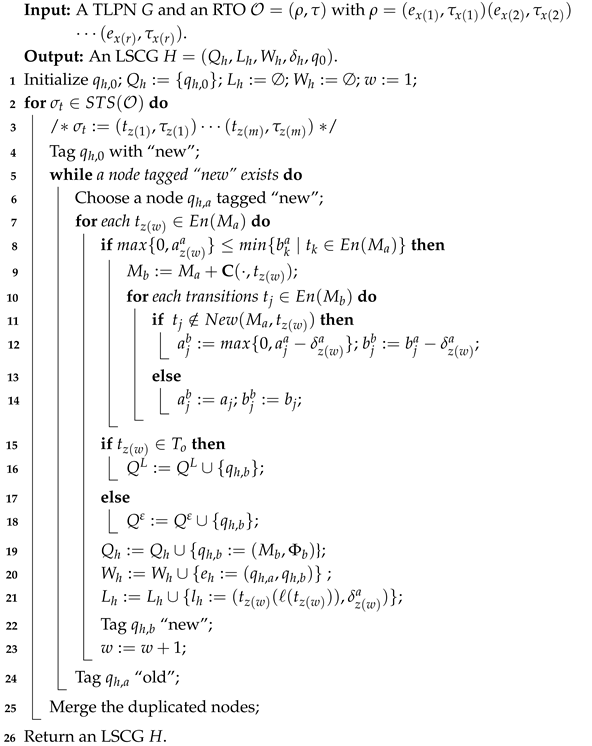
Now, we explain how Algorithm 1 performs. Initially, the set of nodes is initiated by $q_{h,0}$, the sets of edges and labels are empty, and w is set to one (Line 1). A “new” tag is assigned to $q_{h,o}$ (Line 4). In Line 6, a node $q_{h,a}$ is chosen. Each Transition $t_{z\left(w\right)}$ is logically enabled at $M_a$ and must fire after $max\{0,a_z^a\left(w\right)\}$ time units and before $min\{b_k^a\mid t_k\in En\left(M_a\right)\}$ time units (Line 8).

In Line 9, Transition $t_{z\left(w\right)}$ can fire, and a new marking $M_b$ can be obtained. At $M_b$, for all the transitions $t_j$ enabled at $M_b$, if $t_j$ is not newly enabled, its lower and upper bounds are $a_j^b=max\{0,a_j^a-{\delta }_{z\left(w\right)}^a\}$ and $b_j^b=b_j^a-{\delta }_{z\left(w\right)}^a$, respectively; otherwise, the lower and upper bounds of $t_j\in En\left(M_b\right)$ equal to their static closed time intervals (Lines 10–14).

In Lines 15–18, we store the states reached by firing observable and unobservable transitions in $Q^L$ and $Q^{\epsilon }$, respectively. The node $q_{h,b}$, the edge $(q_{h,a},q_{h,b})$, and the label $(t_{z\left(w\right)}(\ell \left(t_{z\left(w\right)}\right)),{\delta }_{z\left(w\right)}^a)$ are added to the sets $Q_h,W_h$, and $L_h$, respectively (Lines 19–21). We choose the tag “new” for $q_{h,b}$ (Line 22). Finally, an LSCG is obtained.

Algorithm 1: Construction of an LSCG

In Algorithm 1, once the transition sequences that are consistent with $\mathcal{O}$ are obtained, we need to search those that are timing consistent with $\mathcal{T}$. In terms of timing consistency, the observation of labels will emerge at the same time instants as in $\rho$ and no further observations will occur until $\tau$ [32].

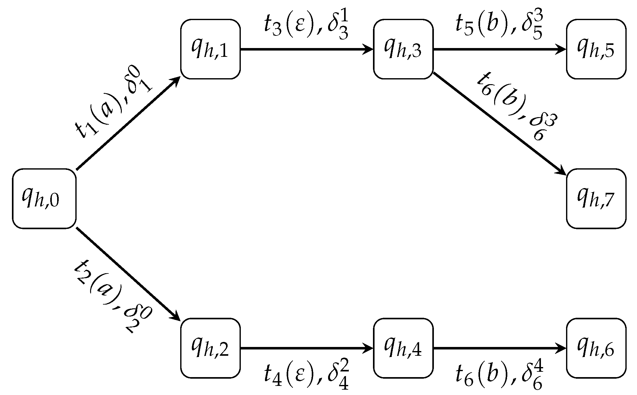
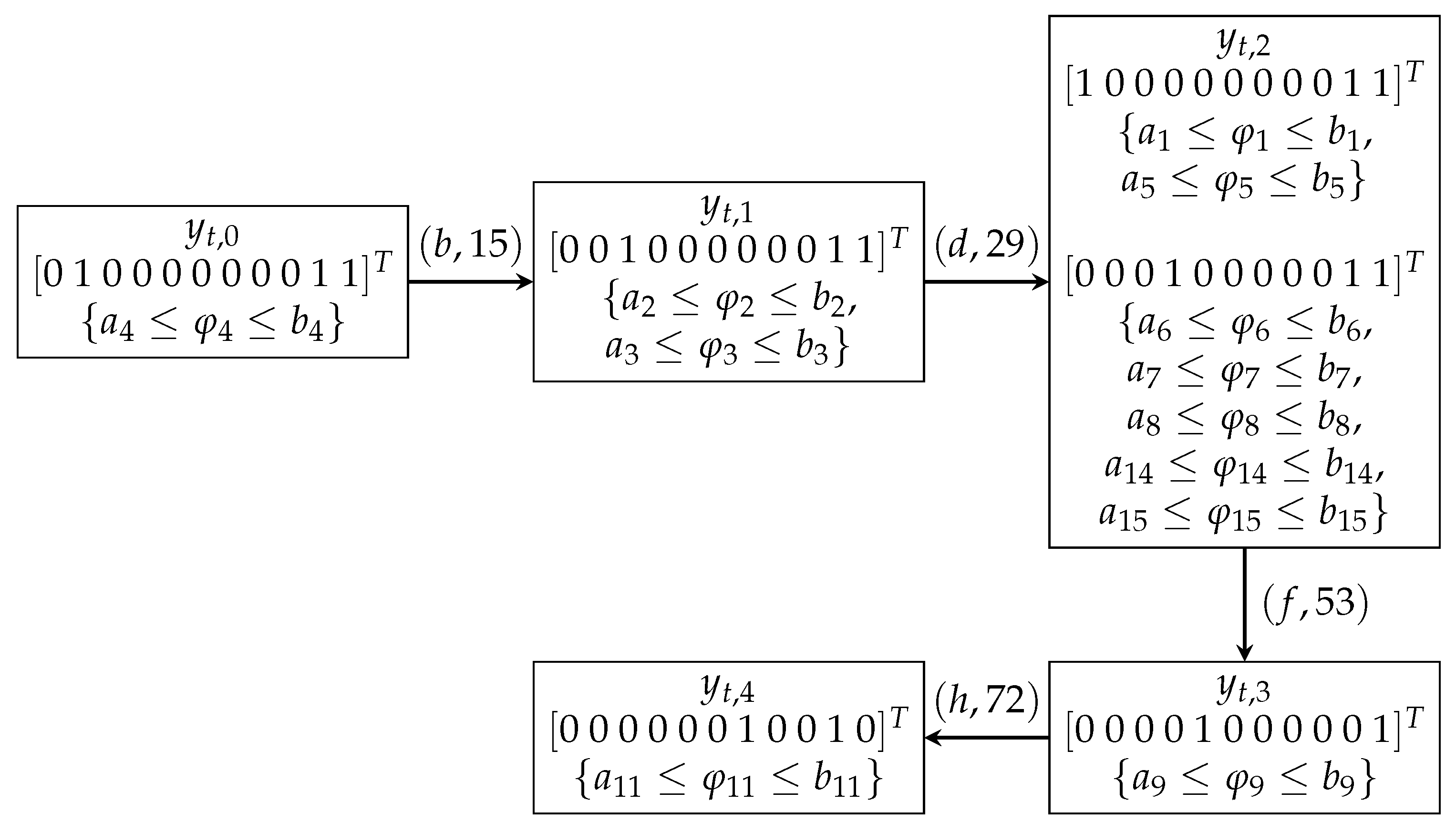
Example 3.

Consider the TLPN G shown in Figure 1 and an RTO $\mathcal{O}=(\rho ,\tau )$ with $\rho =(a,3)(b,10)$ and $\tau =10$. The initial node is $q_{h,0}=({\left[1000000\right]}^T,\{a_1\le {\phi }_1\le b_1,a_2\le {\phi }_2\le b_2\})$ and $En\left(M_0\right)=\{t_1,t_2\}$. We have $\ell \left(t_1\right)=\ell \left(t_2\right)=a$.

At $q_{h,0}$, Transition $t_1$ can fire and yield a marking $M_1={\left[0100000\right]}^T$. Since $t_1$ is observable, by Algorithm 1, the node $q_{h,1}=(M_1,{\mathrm{\Phi }}_1)$ is added to $Q^L$. At $q_{h,1}=(M_1,{\mathrm{\Phi }}_1)$, we have $En\left(M_1\right)=\left\{t_3\right\}$. Since $t_3\in New(M_0,t_1)$, we have ${\mathrm{\Phi }}_1=\{a_3\le {\phi }_3\le b_3\}$. Then, a new node $q_{h,3}=({\left[0001100\right]}^T,\{a_5\le {\phi }_5\le b_5,a_6\le {\phi }_6\le b_6\})$ is generated from $q_{h,1}$ by firing $t_3$. Since $t_3$ is unobservable, the node $q_{h,3}$ is stored in $Q^{\epsilon }$. In a similar way, the remainder of the LSCG can be computed, as shown in Figure 2. Then, by Definition 2, the set of transition sequences consistent with $\mathcal{O}$ is $S\left(\mathcal{O}\right)=\{t_1{t}_3{t}_5,t_1{t}_3{t}_6,t_2{t}_4{t}_6\}$. Moreover, the nodes and firing time units are given in Table 1 and Table 2.

Figure 2. The LSCG with respect to $\mathcal{O}$ of the TLPN in Figure 1.

Table 1. Nodes of the RCSG shown in Figure 2.

Nodes	Markings	Set of Inequalities
$q_{h,0}$	${\left[1000000\right]}^T$	$\{a_1\le {\phi }_1\le b_1$, $a_2\le {\phi }_2\le b_2$}
$q_{h,1}$	${\left[0100000\right]}^T$	$\{a_3\le {\phi }_3\le b_3\}$
$q_{h,2}$	${\left[0010000\right]}^T$	$\{a_4\le {\phi }_4\le b_4\}$
$q_{h,3}$	${\left[0001100\right]}^T$	{$a_5\le {\phi }_5\le b_5$, $a_6\le {\phi }_6\le b_6$}
$q_{h,4}$	${\left[0000100\right]}^T$	$\{a_6\le {\phi }_6\le b_6\}$
$q_{h,5}$	${\left[0000010\right]}^T$	$\{a_7\le {\phi }_7\le b_7\}$
$q_{h,6}$	${\left[0000001\right]}^T$	∅
$q_{h,7}$	${\left[0001001\right]}^T$	∅

Table 2. Firing time units of edges of the LSCG.

Firing Time Units	Transitions	Labels	Time Intervals
${\delta }_1^0$	$t_1$	a	[2, 4]
${\delta }_2^0$	$t_2$	a	[3, 4]
${\delta }_3^1$	$t_3$	$\epsilon$	[4, 8]
${\delta }_4^2$	$t_4$	$\epsilon$	[4, 7]
${\delta }_5^3$	$t_5$	b	[2, 4]
${\delta }_6^3$	$t_6$	b	[3, 4]
${\delta }_6^4$	$t_6$	b	[3, 4]

4. Verification of Detectability Using a Timed State Observer

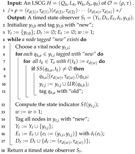
Construction of a Timed State Observer

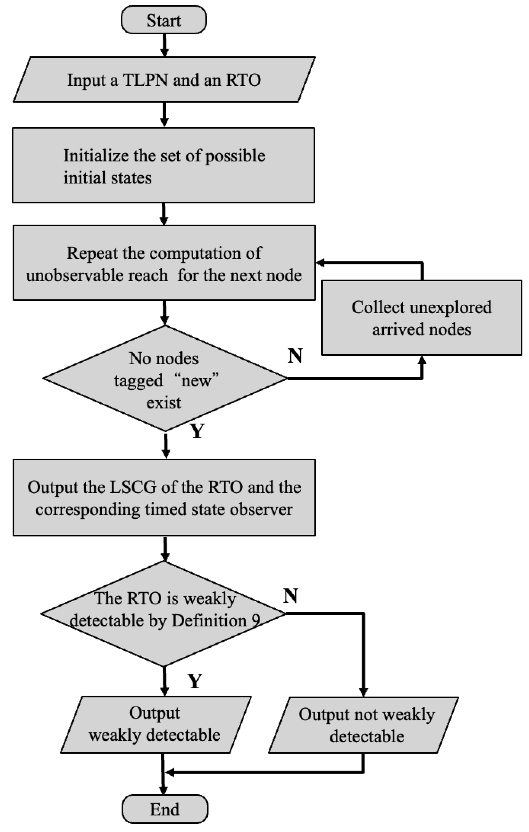
To verify the detectability of a bounded LPN, it is essential to construct an RG and its observer. However, the construction of the observer will unavoidably be affected by the state explosion. In order to address this problem, a timed state observer used to verify state detectability for TLPNs without enumerating all states of a time-dependent system is developed. Specifically, a timed state observer is an observer constructed based on an LSCG that computes the state reached after the occurrence of observable events in order to analyze the detectability of the TLPN systems. Then, the state explosion problem caused by enumerating all states can be addressed. Moreover, to visually represent the proposed algorithm, a concise flowchart for verifying weak detectability is shown in Figure 3.

Figure 3. Flowchart of verifying weak detectability in a TLPN.

Definition 11.

Let $H=(Q_h,L_h,W_h,{\delta }_h,q_0)$ be an LSCG of G with respect to $\mathcal{O}$. A timed state observer $S_t=(Y_t,D_t,E_t,{\delta }_t,y_{t,0})$ is a directed graph, where $Y_t$ is a set of vital nodes, $D_t$ is a set of labels, $E_t\subseteq Y_t\times Y_t$ is a set of edges associated with observable labels, ${\delta }_t$ is a labeling function assigning each edge with a label, and $y_{t,0}$ is the initial vital node.

In an LSCG, the unobservable reach of $q_{h,d}$ is defined as $UR\left(q_{h,d}\right)=\{q_{h,f}\mid \exists {\sigma }_{tu}\in {(T\times {\mathbb{Q}}_0^{+})}^{*}:log\left({\sigma }_{tu}\right)\in T_u^{*},q_{h,d}[{\sigma }_{tu}⟩q_{h,f},q_{h,f}\in Q_r,t_f\left({\sigma }_{tu}\right)\le \tau \}$. Initially, the initial vital node is $y_{t,0}=UR\left(q_{h,0}\right)$ (Line 2). In Line 3, $D_t$ and $E_t$ are empty sets and w is set to one. The vital node $y_{t,i}\in Y_t$ tagged with “new” is chosen in Line 5. For all observable events $t_k\in T_o$ with $\ell \left(t_k\right)=e_{d\left(w\right)}$, we need to compute the subsequent vital nodes after the observable label $e_{d\left(w\right)}$ occurs (Line 7). We must determine whether there exists a transition sequence that fires at $q_{h,a}$ to make an observable Transition $t_k$ occur (Line 8).

If the observable event $e_{d\left(w\right)}$ is enabled at $q_{h,a}$, a new node $q_{h,b}$ will be obtained from $q_{h,a}$ and $y_{t,j}=y_{t,j}\cup UR\left(q_{h,b}\right)$ (Lines 9–10). In Line 11, we tag $q_{h,a}$ with “old”. In Line 12, we compute the state indicator $SI\left(y_{t,j}\right)$ of $y_{t,j}$, i.e., the number of states that are reachable after the occurrence of the label $(e_{d\left(w\right)},{\tau }_{d\left(w\right)})$.

In Line 13, we tag all nodes in $y_{t,j}$ with “new”. New vital nodes are connected with corresponding labels via the addition of edges (Lines 15–17). To be more specific, the vital node $y_{t,j}$, the edge $e_t=(y_{t,i},y_{t,j})$ with ${\delta }_t\left(e_t\right)$, and the label $d_t=(e_{d\left(w\right)},{\tau }_{d\left(w\right)})$ are added to the sets $Y_t$, $E_t$, and $D_t$, respectively. Finally, we obtain a timed state observer.

Example 4.

Let us consider the TLPN G shown in Figure 1, an RTO $\mathcal{O}=(\rho ,\tau )$ with $\rho =(a,2)(b,8)(c,11)$ and $\tau =11$. Initially, we have an initial vital node $y_{t,0}=UR\left(q_{h,0}\right)=\left\{q_{h,0}\right\}$. At $q_{h,0}$, $t_1$ and $t_2$ with $\ell \left(t_1\right)=\ell \left(t_2\right)=a$ are enabled, i.e., $En\left(M_0\right)=\{t_1,t_2\}$. Transition $t_1\left(a\right)$ can fire at $q_{h,0}$ and generate a new node $q_{h,1}$, i.e., $q_{h,0}\stackrel{(t_1\left(a\right),{\delta }_1^0\in [2,4])}{\to }{q}_{h,1}$. By Algorithm 2, $y_{t,1}=y_{t,1}\cup UR\left(q_{h,b}\right)$, we have $y_{t,1}=\{q_{h,1},q_{h,3}\}$ and the state indicator $SI\left(y_{t,1}\right)=2$ is computed, i.e., the number of states that are reachable after the occurrence of the label $(a,2)$. Similarly, we have $y_{t,2}=\left\{q_{h,3}\right\}$ with $SI\left(y_{t,3}\right)=1$, $y_{t,3}=\left\{q_{h,5}\right\}$ with $SI\left(y_{t,3}\right)=1$, and $y_{t,4}=\left\{q_{h,0}\right\}$ with $SI\left(y_{t,4}\right)=1$. We can obtain a timed state observer, as depicted in Figure 4.

Figure 4. The timed state observer of the LSCG with respect to $\mathcal{O}$ in Example 4.

From the timed state observer, a path that can be observed from this observer and is associated with $\mathcal{O}$ is $q_{h,0}\stackrel{(t_1\left(a\right),{\delta }_1^0\in [2,4])}{\to }{q}_{h,1}\stackrel{t_3\left(\epsilon \right),{\delta }_3^1\in [4,8])}{\to }{q}_{h,3}\stackrel{t_5\left(b\right),{\delta }_5^3\in [2,4])}{\to }{q}_{h,5}\stackrel{t_7\left(c\right),{\delta }_7^5\in [3,5])}{\to }{q}_{h,0}$. The transition sequence of this path is $t_1{t}_3{t}_5{t}_7$ with $\ell \left(t_1{t}_3{t}_5{t}_7\right)=abc$. Then, the constraints for this path are as follows.

$$\left\{\begin{array}{c}\begin{array}{c}{\delta }_1^0=2\hfill \\ {\delta }_1^0+{\delta }_3^1+{\delta }_5^3=8\hfill \\ {\delta }_1^0+{\delta }_3^1+{\delta }_5^3+{\delta }_7^5=11\hfill \\ 2\le {\delta }_1^0\le 4\hfill \\ 4\le {\delta }_3^1\le 8\hfill \\ 2\le {\delta }_5^3\le 4\hfill \\ 3\le {\delta }_7^5\le 5\hfill \\ {\delta }_1^0+{\delta }_3^1+{\delta }_5^3+{\delta }_7^5\le 11\hfill \\ 11-({\delta }_1^0+{\delta }_3^1+{\delta }_5^3+{\delta }_7^5)<4\hfill \\ 11-({\delta }_1^0+{\delta }_3^1+{\delta }_5^3+{\delta }_7^5)<5\hfill \end{array}\hfill \end{array}\right.$$

(9)

The above constraints have a solution that is ${\delta }_1^0=2,{\delta }_3^1=4$, ${\delta }_5^3=2$ and ${\delta }_7^5=3$. The state indicator of $y_{t,1}$ is two, as shown in the timed state observer. By Definitions 6, 8, and 9, this RTO $\mathcal{O}=(\rho ,\tau )$ with $\rho =(a,2)(b,8)(c,11)$ and $\tau =11$ is detectable and weakly detectable, but not strongly detectable.

Algorithm 2: Construction of a timed state observer.

Remark 1.

Let $\mathcal{O}=(\rho ,\tau )$ be an RTO with $\rho =(e_{d\left(1\right)},{\tau }_{d\left(1\right)})(e_{d\left(2\right)},{\tau }_{d\left(2\right)})\cdots$$(e_{d\left(n\right)},{\tau }_{d\left(n\right)})$ and $\tau ={\tau }_{d\left(n\right)}$ in G, $H=(Q_h,L_h,W_h,{\delta }_h,q_0)$ be an LSCG of $\mathcal{O}$, and $S_t=(Y_t,D_t,E_t,{\delta }_t,y_{t,0})$ be a timed state observer of H. The RTO $\mathcal{O}$ is strongly detectable if the value of each state indicator is equal to one in $S_t$. This implies that the state of a TLPN system can be uniquely determined after the occurrence of each event in $\mathcal{O}$.

5. Computational Complexity Analysis

To show the contribution of this paper, we analyze the algorithmic complexity of the proposed approach and compare it with the existing methods in this section. In [23], the number of states in an MSCG increases exponentially with the size of a TLPN and its initial marking, since it needs to enumerate all states. In this paper, we construct an LSCG, which is not required to compute all states of a TLPN, to verify the weak and strong detectability of a TLPN. In contrast to an MSCG, the size of the LSCG developed in this paper is related to the length of a given logical label sequence. The proposed method is more efficient since the states calculated by the proposed method are less than or equal to the MSCG. Moreover, a revised state class graph is developed to source the evolution of the RTO in a TLPN for path detectability verification [29]. Verifying path detectability requires searching all paths associated with all prefixes of the RTO. However, in this paper, we only consider states reached after the occurrence of observable events, and the computation of solving for these paths is omitted. Therefore, the approach of this paper is advantageous.

As for Algorithm 1, the maximum number of transitions enabled at a node of an LSCG is $\left|T\right|$. We then compute the number of equations that need to be solved at each node of an LSCG. One equation is needed on Line 9 of Algorithm 1, and $2\left|T\right|$ needs to be solved on Lines 12 and 14 of Algorithm 1. Therefore, the number of equations required to be solved at each node is $2\left|T\right|+1$. Note that if there is no enabled transition at a node, then the computation of the equation for this node is obviated. Let $\mathcal{O}=(\rho ,\tau )$ be an RTO in G. We use $\left|\varsigma \right|$ to denote the length of the longest path associated with $\mathcal{O}$ in the LSCG. Then, the complexity of tracing all paths associated with $\mathcal{O}$ is $O\left(\right|T{|}^{\left|\varsigma \right|})$. In the worst case, each transition in a path is observable. The complexity of tagging the nodes reached after the occurrence of an observable transition in a path is $\left|\varsigma \right|$. For the path associated with $\mathcal{O}$, the total number of constraints equals $3\left|\varsigma \right|+\left|T\right|\left(\right|\varsigma |+1)+1$, at most. Note that the number of constraints for checking the enabled transitions of the last node is equal to $\left|T\right|$, at most.

Then, we show the complexity of Algorithm 2. Particularly, Line 1 in Algorithm 2 only needs to compute the unobservable reach of the initial node. Hence, the complexity is $O\left(\right|T{|}^{|{\zeta }_u|})$, where $|{\zeta }_u|$ is the length of the longest unobservable path from the initial node. Moreover, the complexity of finding the unobservable reach of a node reached by the occurrence of an observable event $e_{d\left(w\right)}$ is $O\left(\right|T{|}^{|{\zeta }_e|})$, where $|{\zeta }_e|$ is the longest unobservable path from this node. In the worst case, the complexity of solving the state indicator is $|Y_t|$. The complexity of checking that a path is consistent with the labels of the timed state observer is $O\left(\right|E_t\left|\right)$.

6. Case Study

We consider an intelligent garage system, as shown in Figure 5, which consists mainly of an automatic barrier gate, a monitor, a wireless sensor, and so forth. The private smart garage generally parks a sport utility vehicle (SUV) and a sedan, which are occupied by a male and female owner, respectively. Intelligent garage systems deliver personalized services and energy-saving strategies for different vehicles: for instance, the smart adjustment of the height of the garage door, burglary alerts, and intelligent standby, etc. The smart garage system is modeled by a TLPN, which is shown in Figure 6.

Figure 5. Intelligent garage system.

Figure 6. TLPN model of an intelligent garage system.

The system is turned off after 14–18 s (Transition $t_3$) when the couple leaves for work at 9:30 and is in the shutdown state (Place $p_1$). The system enters from the shutdown state to the standby state (Place $p_2$) after 14–20 s at 17:30 for the end of the workday of this couple (Transition $t_4$). When a vehicle is detected in front of the automatic barrier gate, the system enters the activated state (Place $p_0$) for 12–25 s (Transition $t_2$); otherwise, it enters the standby state (Place $p_2$) to enable the energy-saving strategy.

When a vehicle is preparing to enter the private garage, it is detected by the automatic barrier gate within 8–16 s (Transition $t_5$). The system enters the detected state (Place $p_3$). If this vehicle is not licensed by the owners, then the system will return to the standby state and alert with a message in 15–26 s (Transition $t_6$). If this vehicle is licensed by the owners, then its type will be confirmed, which requires 14–22 s of detection for an SUV (Transition $t_7$) and 14–20 s of detection for a sedan (Transition $t_8$). For an SUV, after the detection is complete, its vehicle identification chip is verified by the wireless sensor (Place $p_4$) to ensure security, and then the smart adjustment of the garage door and the personalized temperature service are provided for the vehicle and driver. An SUV is higher than a sedan, which means it requires a longer time to open the garage door. This intelligent garage system requires 18–32 s (Transition $t_9$) to open the garage door for an SUV and 12–22 s for a sedan (Transition $t_{10}$). Similarly, the time intervals to close the door for an SUV and a sedan are 28–42 s (Transition $t_{11}$) and 18–32 s (Transition $t_{12}$), respectively. Places $p_9$ and $p_{10}$ ensure that only one vehicle is detected each time. Finally, the vehicle enters into the garage (Place $p_8$) and the garage door is closed (Transition $t_{13}$). Moreover, Transitions $t_{14}$ and $t_{15}$ indicate the potential delay incurred by the sensor, i.e., more time may be required for detection.

Based on the TLPN model of the intelligent garage system, the set of labels is $E=\{a,b,c,d,e,f,g,h,i,j,k\}$, $T_o=\{t_1,t_2,t_3,t_4,t_6,t_7,t_8,t_9,t_{10},t_{11},t_{12}\}$, where $\ell \left(t_1\right)=c$, $\ell \left(t_2\right)=d$, $\ell \left(t_3\right)=a$, $\ell \left(t_4\right)=b$, $\ell \left(t_6\right)=e$, $\ell \left(t_7\right)=\ell \left(t_{14}\right)=f$, $\ell \left(t_8\right)=\ell \left(t_{15}\right)=g$, $\ell \left(t_9\right)=h$, $\ell \left(t_{10}\right)=i$, $\ell \left(t_{11}\right)=j$, and $\ell \left(t_{12}\right)=k$, with $I\left(t_1\right)=[12,25]$, $I\left(t_2\right)=[12,25]$, $I\left(t_3\right)=[14,18]$, $I\left(t_4\right)=[14,20]$, $I\left(t_5\right)=[8,16]$, $I\left(t_6\right)=[15,26]$, $I\left(t_7\right)=[14,22]$, $I\left(t_8\right)=[14,20]$, $I\left(t_9\right)=[18,32]$, $I\left(t_{10}\right)=[12,22]$, $I\left(t_{11}\right)=[28,42]$, $I\left(t_{12}\right)=[18,32]$, $I\left(t_{13}\right)=[14,22]$, $I\left(t_{14}\right)=[16,24]$, and $I\left(t_{15}\right)=[16,24]$. The initial state $q_{h,0}=(M_0,{\mathrm{\Phi }}_0)$, where $M_0={\left[01000000011\right]}^T$ and ${\mathrm{\Phi }}_0=\{a_4\le {\phi }_4\le b_4\}$.

Suppose the intruder observes the process of a certain vehicle entering the garage, i.e., an RTO $\mathcal{O}$ with $\rho =(b,15)(d,29)(f,53)(h,72)$ and $\tau =72$. Constructing a timed state observer using Algorithm 2, we can obtain $y_{t,0}\stackrel{(b,15)}{\to }{y}_{t,1}\stackrel{(d,29)}{\to }{y}_{t,2}\stackrel{(f,53)}{\to }{y}_{t,3}\stackrel{(h,72)}{\to }{y}_{t,4}$. After the occurrence of the event pair $(d,29)$, there are two states in $y_{t,2}$, which means that the value of the corresponding state indicator exceeds one. The timed state observer is shown in Figure 7. From this observer, it can be seen that the proposed method for detectability verification is still effective when sensor delays are considered. In other words, after observing the system entering the activated state, the intruder cannot determine whether the system is currently in the activated or detected state. Therefore, by Definition 8, the RTO is not strongly detectable; however, by Definition 9, it is weakly detectable.

Figure 7. The timed state observer of the LSCG with respect to $\mathcal{O}$ in the intelligent garage system.

7. Conclusions

In this paper, strong and weak detectability are defined in a TLPN. We develop an LSCG, which is not required to enumerate all states of a system, to compute the states with respect to a given RTO. Then, with the proposed LSCG, an information structure called a timed state observer is developed. Based on the timed state observer, strong and weak detectability properties can be efficiently verified in TLPNs. Since only one timed state observer needs to be constructed, these two types of detectability can be verified at the same time by checking the state indicators of the timed state observer. In the prospective work, we are intrigued to consider the initial state estimation problem in TLPNs under time constraints.