Dynamical Properties for a Unified Class of One-Dimensional Discrete Maps

Abstract

Currently, despite advances in the analysis of dynamical systems, there are still doubts about the transition between both stable and chaotic behaviors. In this research, we will explain the transition of a system that develops between two dynamic systems that have already been studied: the classical logistic model and a new chaotic system. This research addresses the study of the transition of both the system and its behaviors using computational techniques, where cobweb diagrams, time series, bifurcation diagrams, and even a graphical visualization for the maximum Lyapunov exponent will be visualized. Using a graphical and numerical methodology, bifurcation points were identified that revealed the transition of behaviors at different points. This resulted in a deep understanding of the dynamics of the system, thus highlighting the importance of incorporating computational analysis in dynamic systems, which greatly contributes to the efficient modeling of natural phenomena.

1. Introduction

In this paper, we study the transition between the following discrete maps:

$$x_{n+1}=\mu x_n(1-x_n)$$

(1)

and

$$x_{n+1}={\displaystyle \frac{\mu x_n(1-x_n)}{1+x_n}},$$

(2)

where $0<\mu <1$ and $x_n\in [0,1].$

Equation (1) corresponds to the well-known discrete logistic equation. R. May proposed it [1] in 1976, and it has been deeply studied due to being the reference toy model that is used to explore the properties of one-dimensional discrete dynamical systems. Some recent references include [2,3,4] (this list being by no means exhaustive). Map (2) was recently introduced by Kumar et al. in reference [5], where some dynamical properties, including fixed points, attracting points, repelling points, and the stability and chaotic behavior of this map, were analyzed. With the help of bifurcation diagrams, it was proved in [5] that the range of stability and chaos of the dynamical system (2) is larger than that of (1). Such a model has been already used to improve secure image encryption in [6] (see also [7,8]). Inspired by this model, Renu and Chugh studied the stability of the modified model

$$x_{n+1}=(1-\eta )x_n+\eta {\displaystyle \frac{\mu x_n(1-x_n)}{1+x_n}},$$

(3)

as presented in [9,10], thereby showing the superior stability performance of this discrete system. Additionally, the stability and chaos of the deformed model

$$x_{n+1}={\displaystyle \frac{\mu x_n(1-x_n+\epsilon (1-x_n))}{(1+\epsilon (1-x_n))+((1+x_n)+\epsilon (1-x_n))}}$$

(4)

was also analyzed in [11]. Recent fractional discrete dynamical systems were also studied in [12].

It should be noted that the construction of discrete chaotic maps, their dynamical analysis, and pertinent applications have consistently constituted highly prevalent research topics. Some relevant and recent references include, but are not limited to [13,14,15,16].

Since the structures of Equations (1) and (2) are algebraically different, it is natural to ask what happens to their dynamics if we try to make a continuous transition between both maps. We will investigate to what extent and how the range of stability and chaos changes when we move from one map to another. We will also establish patterns and draw conclusions about the dynamic properties of our proposed generalized extended map.

This paper aims to give a plausible answer to this question. For that purpose, we propose studying the following model:

$$x_{n+1}={\displaystyle \frac{\mu x_n(1-x_n)}{1+\lambda x_n}},$$

(5)

where $\lambda \in [0,1]$. Our methods are based on a qualitative study using graphs showing the effect of the arbitrary transition parameter on the number of equilibrium points, their locations, stability conditions, cobweb plots, time series diagrams, and bifurcation diagrams of chaotic behavior.

Surprisingly, both applications were closer than we might have initially assumed from the results previously shown in [5]. This new finding allows us to conclude that both systems behave similarly, providing a new modifiable parameter that increases the degree of freedom and flexibility of the discrete logistic equation.

This paper is organized as follows: In Section 2, we provide an analytic characterization of the fixed points. Cobweb and time series diagrams are depicted in Section 3 and Section 4, respectively. In Section 5, we present several bifurcation diagrams for different values of $\lambda$. The maximal Lyapunov exponents are shown in Section 6, and, through overlapping the bifurcation diagrams with maximal Lyapunov exponents, we obtained the bifurcation points, as shown in Section 7. Finally, some conclusions are drawn in Section 8.

2. Existence of Fixed Points

In this section, we present some results that will be needed throughout the paper on the existence of sufficient conditions for the characterization of the fixed points of Equation (5). For a general reference of the analysis of discrete dynamical systems, we referred to [17,18].

Theorem 1.

Suppose that $\mu >0$ and $0\le \lambda \le 1.$ Then, the unique fixed points associated with System (1) are $x_1=0$ and $x_2={\displaystyle \frac{\mu -1}{\mu +\lambda }}.$ Moreover, we can also conclude the following:

(i) 

The fixed point $x_1$ is attracting (or stable) if $0<\mu <1$ and repelling (or unstable) if $\mu >1;$

(ii) 

If $\mu >1$, the fixed point $x_2$ is

(a) 

attracting if

$$\mu <{\displaystyle \frac{(\lambda +3)+\sqrt{(\lambda +1)(\lambda +9)}}{2}}$$

(b) 

repelling if

$${\displaystyle \frac{(\lambda +3)+\sqrt{(\lambda +1)(\lambda +9)}}{2}}<\mu .$$

Proof. 

We will first prove that, under the given hypothesis, the fixed points are $x_1=0$ and $x_2={\displaystyle \frac{\mu -1}{\mu +\lambda }}.$ Indeed, we have

$${\displaystyle \frac{\mu x(1-x)}{1+\lambda x}}=x,$$

if and only if

$$x\left[\right(\mu -1)-x(\mu +\lambda \left)\right]=0.$$

Hence, we have two possible cases:

$$x=0\mathrm{and}(\mu -1)-x(\mu +\lambda )=0.$$

When developing the right hand side, we obtain

$$x={\displaystyle \frac{\mu -1}{\mu +\lambda }}.$$

We next used the following well-known criteria: Let $x^{*}$ be a fixed point of the map $\mathcal{K}$, then.

• If $|{\mathcal{K}}^{\prime }\left(x^{*}\right)|<1$, then the fixed point $x^{*}$ is attracting.
• If $\left|\mathcal{K}\right(x^{*}\left)\right|>1$, then the fixed point $x^{*}$ is repelling.

We then have

$${\mathcal{K}}^{\prime }\left(x\right)={\displaystyle \frac{\mu -2\mu x-\lambda \mu x^2}{{(1+\lambda x)}^2}}={\displaystyle \frac{\mu }{{(1+\lambda x)}^2}}(1-x)-{\displaystyle \frac{\mu }{(1+\lambda x)}}x.$$

(6)

Hence, $|{\mathcal{K}}^{\prime }\left(0\right)|=\mu$ and $\left(i\right)$ follow. On the other hand, since, for $x_2={\displaystyle \frac{\mu -1}{\mu +\lambda }}$, we have $1+\lambda x_2={\displaystyle \frac{\mu (1+\lambda )}{\mu +\lambda }}$ and $1-x_2={\displaystyle \frac{1+\lambda }{\mu +\lambda }},$ we obtain

$${\mathcal{K}}^{\prime }\left(x_2\right)={\displaystyle \frac{\mu {(\mu +\lambda )}^2}{{\mu }^2{(\lambda +1)}^2}}{\displaystyle \frac{\lambda +1}{\mu +\lambda }}-{\displaystyle \frac{\mu (\mu +\lambda )}{\mu (1+\lambda )}}{\displaystyle \frac{\mu -1}{(\mu +\lambda )}}={\displaystyle \frac{1}{\mu (\lambda +1)}}[\lambda +2\mu -{\mu }^2].$$

(7)

Consequently, $|{\mathcal{K}}^{\prime }\left(x_2\right)|<1$, i.e., $x_2$, is attracting if and only if

$$-\mu (\lambda +1)<2\mu +\lambda -{\mu }^2<\mu (\lambda +1).$$

(8)

The inequality on the right hand side shows that

$$0<{\mu }^2+\mu (\lambda -1)-\lambda =(\mu -1)(\mu +\lambda ),$$

(9)

which implies that necessarily $\mu >1$.

The inequality on the left hand side of Equation (8) shows that

$$\left(\mu -{\displaystyle \frac{(\lambda +3)+\sqrt{(\lambda +1)(\lambda +9)}}{2}}\right)\left(\mu -{\displaystyle \frac{(\lambda +3)-\sqrt{(\lambda +1)(\lambda +9)}}{2}}\right)={\mu }^2-(\lambda +3)\mu -\lambda <0.$$

(10)

Since $0\le \lambda \le 1$, we obtain ${\displaystyle \frac{3}{2}}-\sqrt{5}\le {\displaystyle \frac{(\lambda +3)-\sqrt{(\lambda +1)(\lambda +9)}}{2}}\le {\displaystyle \frac{1}{2}}<\mu$ and hence necessarily $\mu <{\displaystyle \frac{(\lambda +3)+\sqrt{(\lambda +1)(\lambda +9)}}{2}}$, which proves $\left(a\right)$.

For Case $\left(b\right),$ and from (8), we must have $|{\mathcal{K}}^{\prime }\left(x_2\right)|>1$, that is,

$$2\mu +\lambda -{\mu }^2>\mu (\lambda +1)\mathrm{o}\mathrm{r}-\mu (\lambda +1)>2\mu +\lambda -{\mu }^2.$$

(11)

In the first case, it follows from the reverse inequality in (9) that necessarily $\mu <1$, which contradicts our assumption on $\mu .$ In the second case, we have again $\mu >{\displaystyle \frac{1}{2}}>{\displaystyle \frac{(\lambda +3)-\sqrt{(\lambda +1)(\lambda +9)}}{2}}$; hence, from the reverse inequality in (10), we can conclude that $\left(b\right)$ holds. □

3. Cobweb Plots

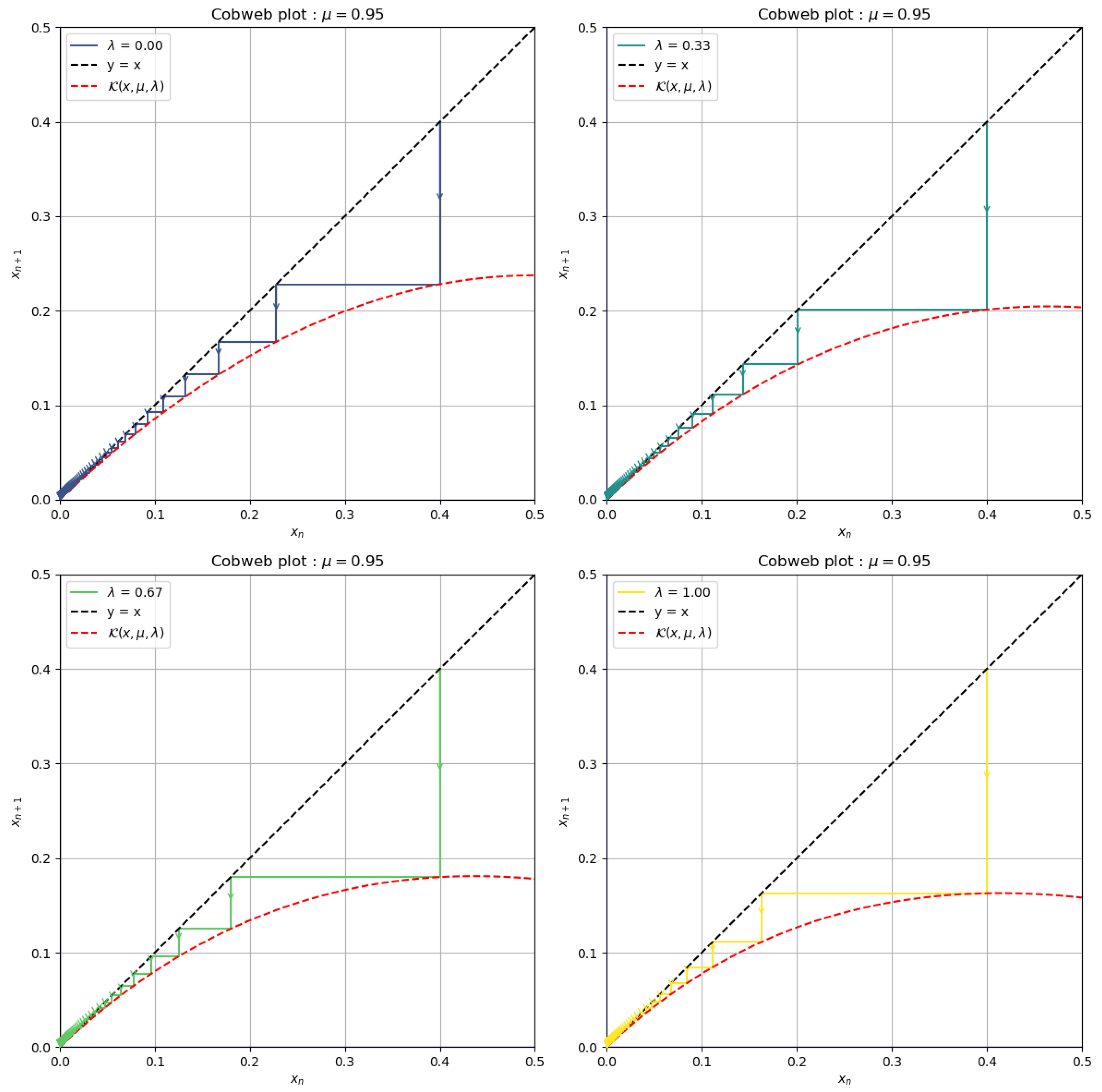
Cobweb plots are a valuable graphical tool in the study of dynamical systems. As a visual method, the cobweb plot allows one to explore the evolution of an iterative sequence in a two-dimensional plane, thus providing detailed information about the behavior over time. In the context of one-dimensional chaotic systems, the cobweb plot is used to illustrate how successive points in the iterative sequence relate to each other, where each point in the plot represents a state of the system at a given instant of time and where the lines connecting these points in chronological order create a cobweb structure.

The main objective of this plot is to show the convergence or divergence of the iterative sequence and reveal patterns, which is directly related to the identification of fixed points since, through the image, it can be revealed whether, as time passes, there are or are not converging toward specific points, which provides information about the stability of a system.

Cobweb plots for Map $\mathcal{K}$ will be presented below. The plots will consist of four subgraphs, in which there will be four equidistant values of $\lambda$ in order to obtain an overview of how the values change as $\lambda$ increases.

3.1. Examples of Cobweb Plots for $\mu \in (0,1)$

Figure 1 shows Map $\mathcal{K}$ for four equally spaced values of $\lambda$ in order to understand what happens as $\lambda$ increases. It can be seen that all graphs converge toward the fixed point $x_1=0$, which coincides with the analytical results.

3.2. Example of Cobweb Plots for $\mu >1$

We start with the following case $\mu =1.5$.

3.2.1. Examples of Cobweb Plots for $\mu =1.5$

Figure 2 shows that, for four different values of $\lambda$, repelling behaviors of the fixed point $x_1=0$ are drawn. However, it can be deduced from this result that, although the diagram shows repelling behavior for the fixed point $x_1=0$, it shows flow lines in the direction of the fixed point $x_2={\displaystyle \frac{\mu -1}{\mu +\lambda }}$. This is because there is precisely an attracting behavior toward that fixed point, but whenever it is true, the following applies:

$$1<\mu <{\displaystyle \frac{(\lambda +3)+\sqrt{(\lambda +1)(\lambda +9)}}{2}}.$$

(12)

3.2.2. Example of Cobweb Plots for $\mu =3.3$

Figure 3 shows that, for $\lambda =0$, a behavior was found that is not attractive toward any point. However, we can begin to see a possible periodic behavior. This is because the flow lines follow a defined pattern. On the other hand, $\lambda =0.33$, $\lambda =0.67$, and $\lambda =1$ all exhibited attracting behavior.

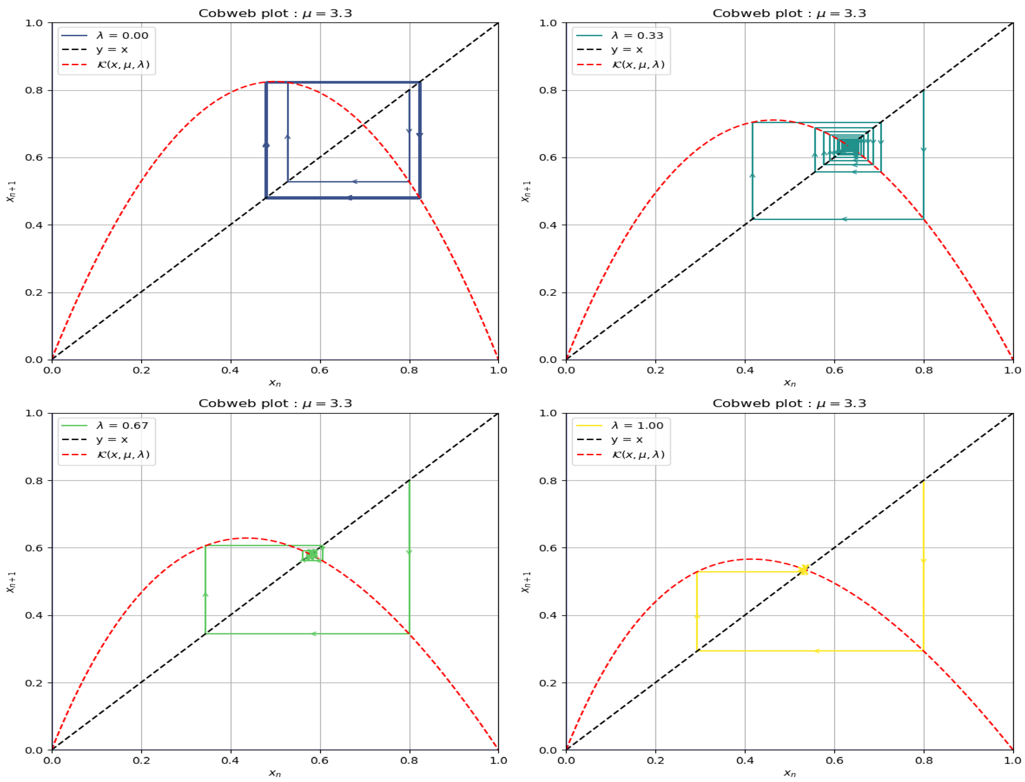
3.2.3. Examples of Cobweb Plots for $\mu =3.5$

In Figure 4, we can see much more defined periodic behavior for both $\lambda =0$ and $\lambda =0.33$. In contrast, the other values continued to have an attracting behavior, corroborating the previous analytical results.

We finish this section with the case $\mu =4$.

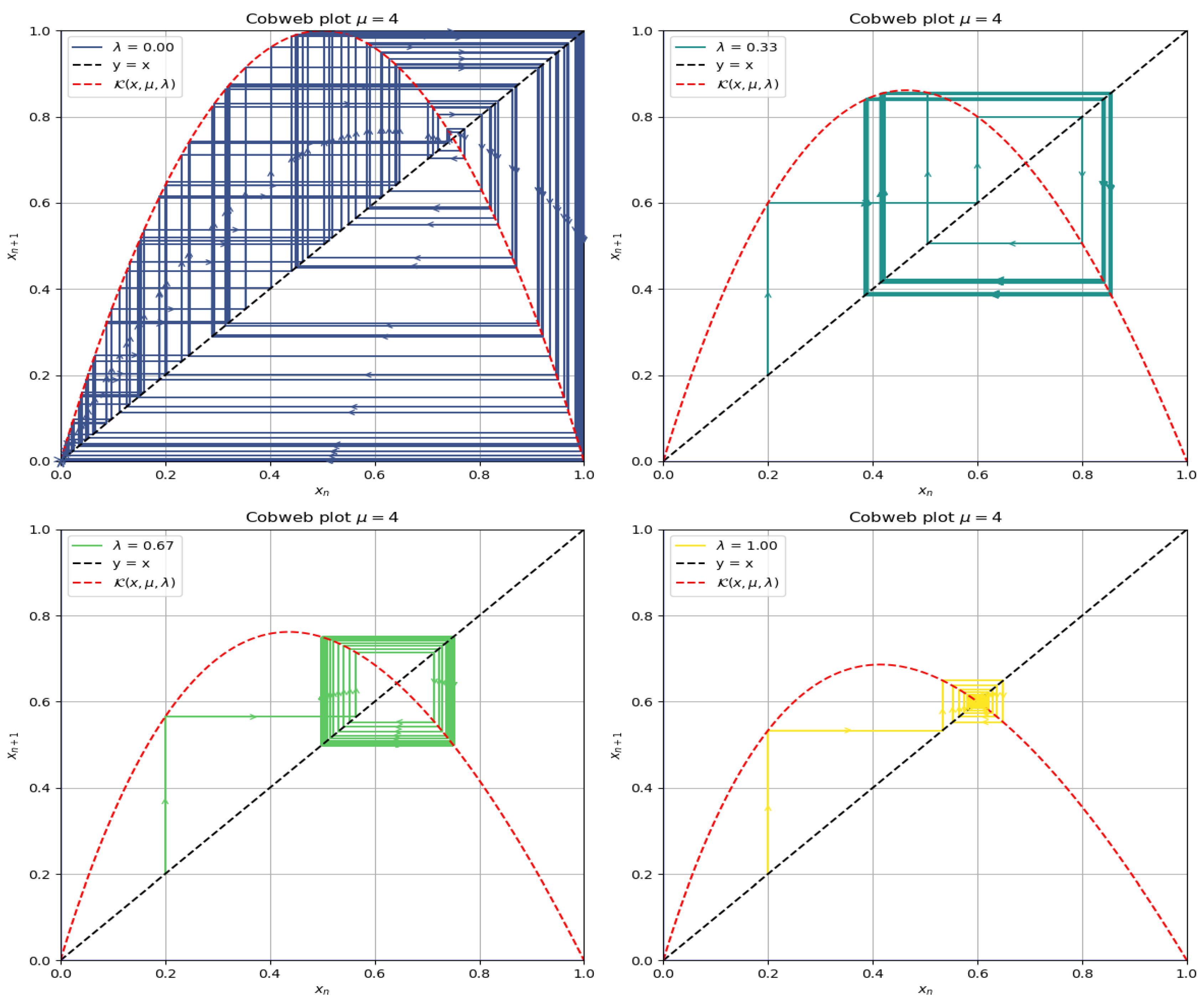
3.2.4. Examples of Cobweb Plots for $\mu =4$

From Figure 5, we can already notice a first approach toward chaotic behavior according to the graph presented for the value $\lambda =0$. On the other hand, attracting behavior was shown for $\lambda =1$. The above confirms what the analytical results revealed but opens the question regarding periodic stable behavior. In the next section, we will study if there is any type of periodicity through a graphic study using the time series diagram.

4. Time Series Diagrams

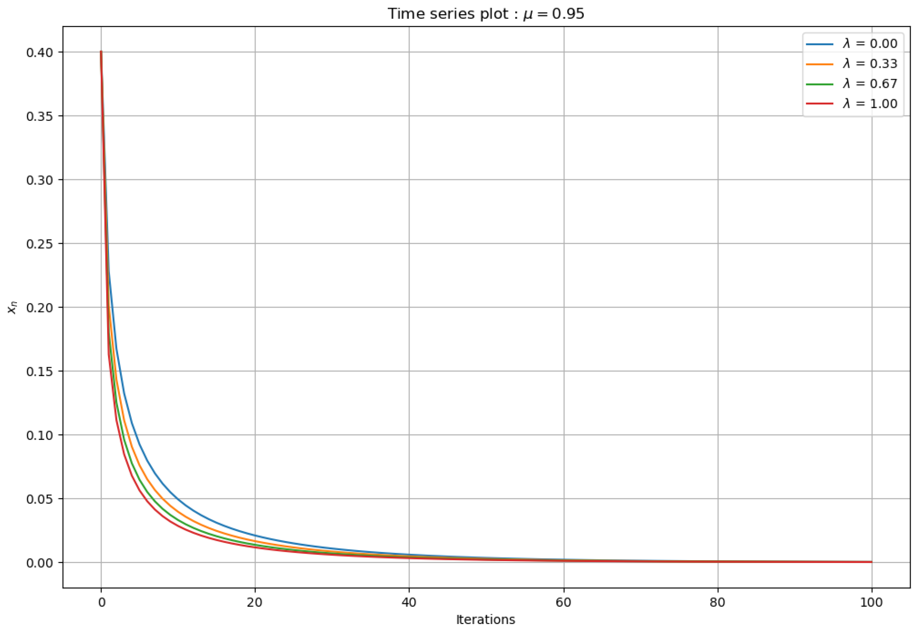
The time series diagram is a tool for exploring and understanding dynamical systems. Its primary function is to provide a graphical approach to the temporal evolution of a variable since, thanks to this, the system’s patterns, trends, and behaviors can be revealed. This type of graph is of great importance for the study of one-dimensional maps since it provides a temporal vision of the trajectories of the system being analyzed. In mathematical terms, the time series diagram is the ordered sequence of values of a variable over discrete time intervals.

Graphically, this diagram takes the number of iterations on the horizontal axis and the values corresponding to the study variable on the vertical axis, that is, each point of the drawn line will reflect the system’s state in a specific iteration. Regarding the usefulness of these diagrams in one-dimensional chaotic systems, they mainly serve to visualize and understand the dynamics present in the map in question. As a graph, it makes it possible to identify specific behaviors as the system develops over time, thus allowing for analyses of the stability, variability, and the presence of recurring or chaotic patterns.

In a similar way as in the previous section, we analyzed different cases in terms of the values of the parameters $\mu$ and $\lambda$.

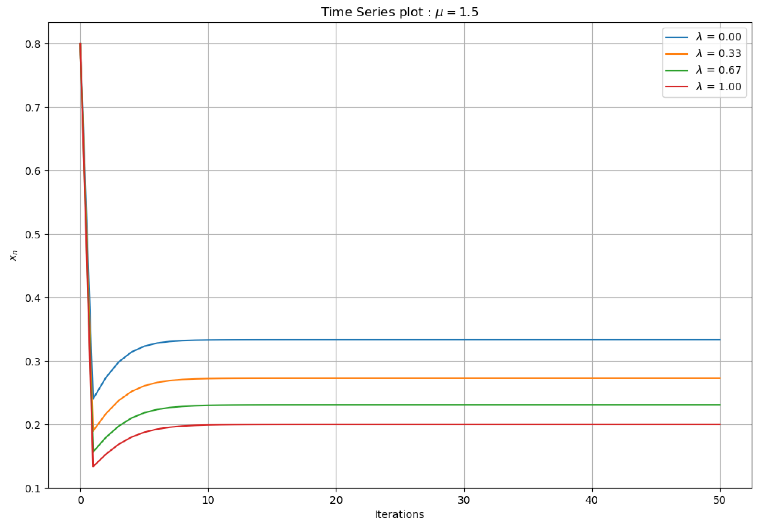
4.1. Examples of Time Series Diagrams for $\mu \in (0,1)$

As shown in Figure 6, it was observed that, with each iteration, the system tended toward the value 0, which indicates that there is an attracting behavior toward the fixed point $x_1=0$, with $\mu \in (0,1)$. Furthermore, no signs of periodic behavior were detected on the map.

4.2. Examples of Cobweb Plots for $\mu >1$

We continued with the same sequence of values from the previous section.

Examples of Time Series Diagrams for $\mu =1.5$

As seen in Figure 7, there was repelling behavior for the fixed point $x_1=0$.

4.3. Examples of Time Series Diagrams for $\mu =3.3$

As seen in Figure 8, there were only three attracting behaviors. These behaviors will be for all values of $\lambda$ except $\lambda =0$, which can be seen to have an oscillating behavior with convergence toward two particular points. This happens because, when $\mu =3.3$, a double-period bifurcation appears, that is, the fixed point loses its stability and begins an attractor orbit of Period 2. The above could be the first indication of the existence of periodic stable behavior and also of the presence of bifurcations within the map.

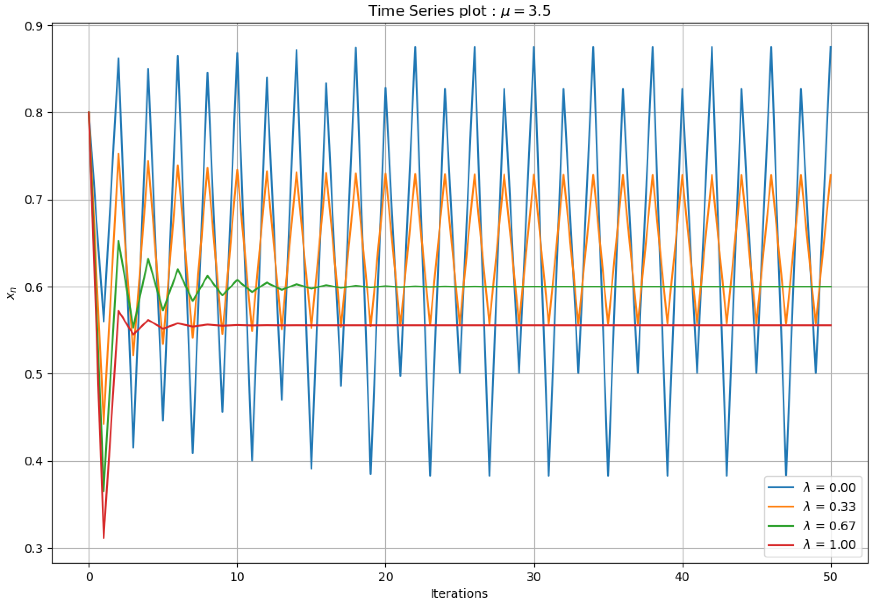
4.4. Examples of Time Series Diagrams for $\mu =3.5$

As shown in Figure 9, for the values $\lambda =0$ and $\lambda =0.33$, periodic behavior could be observed, but, for the other two values, attracting behavior was still obtained.

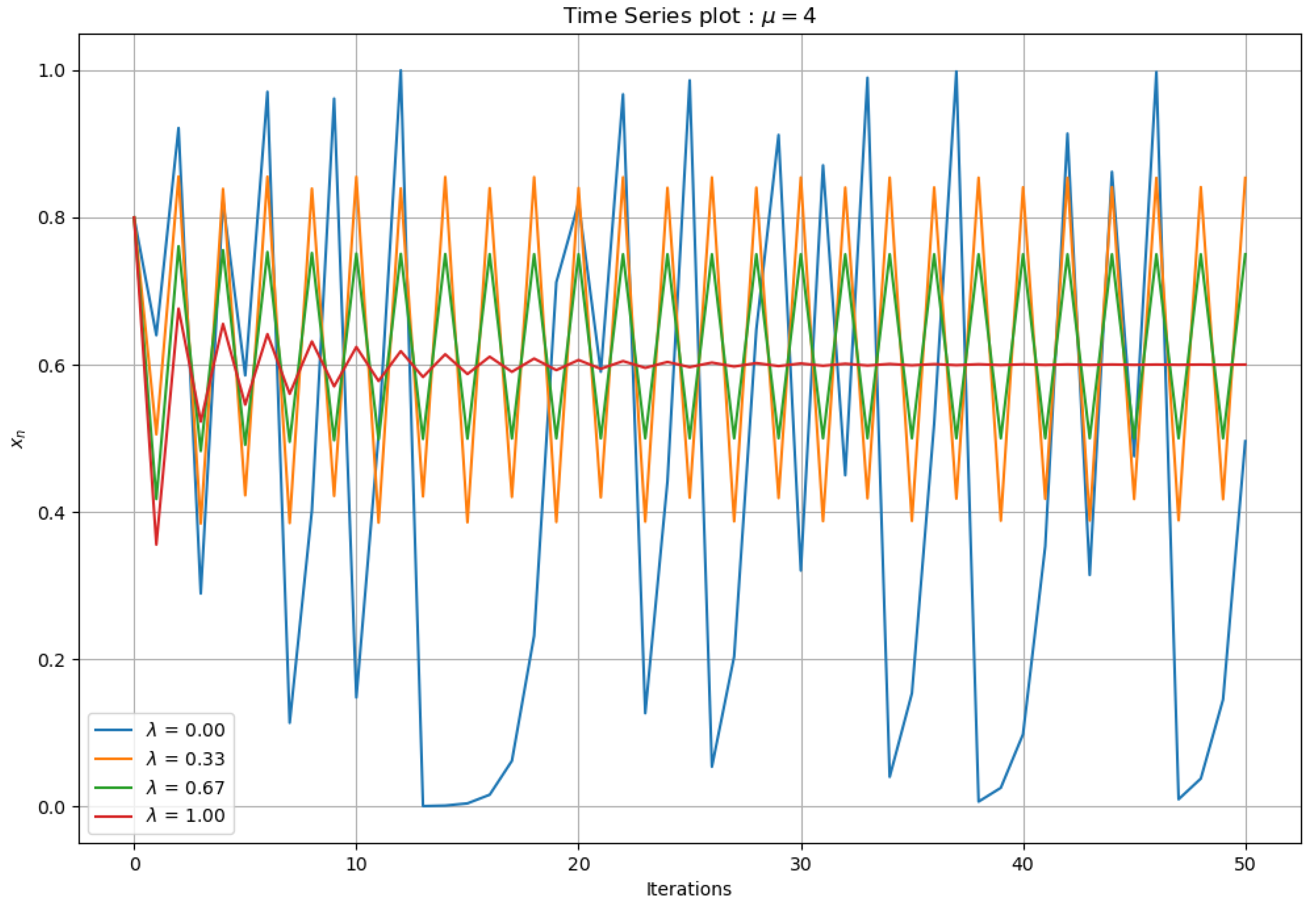
4.5. Examples of Time Series Diagrams for $\mu =4$

Figure 10 shows attracting behavior for $\lambda =1$. In contrast, for $\lambda =0.33$ and $\lambda =0.67$, there was periodic behavior, where it can be seen that each one had a different period, which appears to be of Periods 2 and 4, respectively. Finally, it was observed that, for $\lambda =0$, despite having specific patterns, these were not defined by iteration so that one could speak of apparent periodic behavior.

With the graphical results obtained in the time series diagrams, the question arises whether it is possible to determine the values of $\mu$ that change the map from stable behavior to stable periodic behavior, as well as from stable periodic behavior to chaotic behavior. This can be studied through the bifurcation diagram, which will provide a graphical approximation of these values.

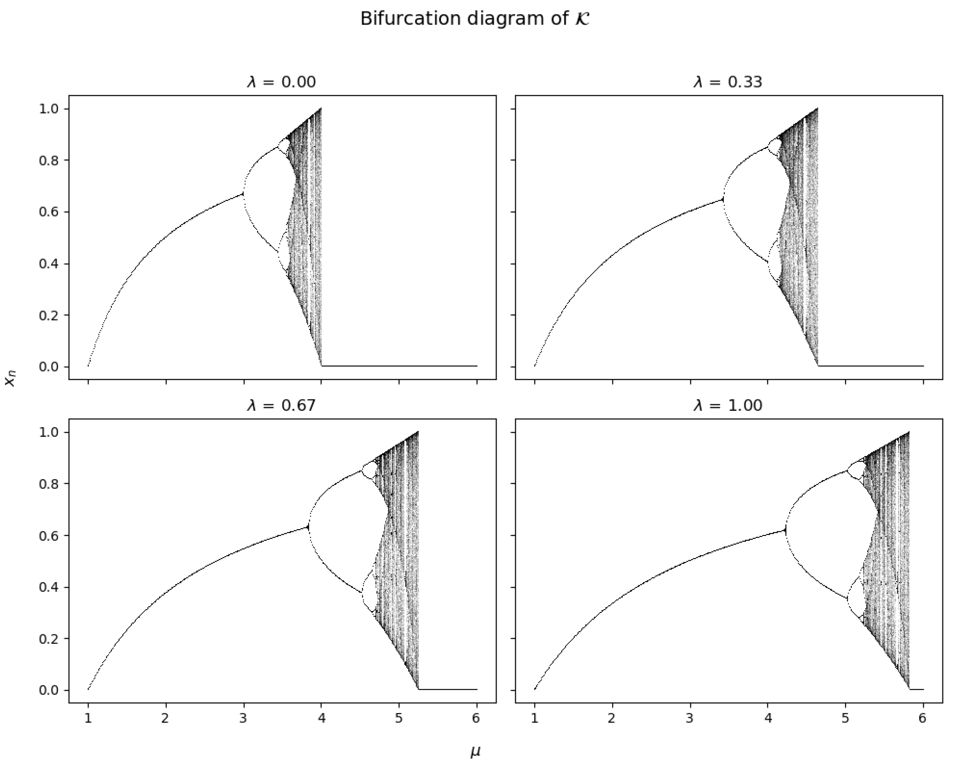
5. Bifurcation Diagrams

The bifurcation diagram is an important graphical tool for exploring the complexity and behavioral transitions in dynamical systems. Mathematically, the bifurcation diagram plots a system’s stationary or periodic solutions as a function of a specific parameter, revealing the structure and organization of the stationary states of the system. In other words, the graph provides a picture of how the system behaves about the variation of the initial conditions or its parameters. This graphical representation is essential to identify the regions of stability and to understand in which sector the chaotic behavior of the studied system begins.

As shown in Figure 11, a great similarity can be noted between the graphs as $\lambda$ changes while maintaining the same structure. The biggest difference lay in a notable translation between each of the graphs, which motivated finding the bifurcation points (or an approximation) that are present in the graph, at least in its first periods, in order to determine the stability intervals, periodic stability, and unpredictable or highly sensitive behavior to the initial conditions.

6. Maximal Lyapunov Exponent

The maximal Lyapunov exponent is a fundamental tool for studying nonlinear dynamical systems since it helps to understand the sensitivity to initial conditions and, therefore, the chaotic nature of dynamical systems. Mathematically, this exponent quantifies the average rate of divergence or convergence of the trajectories close to the phase space. Thus, the maximal Lyapunov exponent is defined as

$$\sigma =\underset{n\to \infty }{lim}{\displaystyle \frac{1}{n}}\sum _{i=0}^{n-1}log\left|{\mathcal{K}}^{\prime }\left(x_i\right)\right|,$$

(13)

where ${\mathcal{K}}^{\prime }\left(x_i\right)$ represents the derivative of the function $\mathcal{K}$ evaluated at the point $x_i$ of the trajectory. This exponent provides information about the system’s stability, where a positive value of $\sigma$ indicates exponential divergence for nearby trajectories, suggesting chaotic behavior. On the other hand, a negative exponent will signal a convergence toward an attracting point, thus offering more stable behavior. Referring to chaotic systems, it can be said that at least one positive exponent could confirm the sensitivity to initial conditions; this means that the maximal Lyapunov exponent is an excellent quantifier of the sensitivity to initial conditions in this type of system.

In the case of one-dimensional chaotic systems, the graph of the maximal Lyapunov exponent can show transitions from ordered to chaotic behavior. With the graphs, one can observe peaks that indicate the presence of bifurcation points, where the system goes from behaving regularly to chaotic. Furthermore, this exponent allows us to identify the presence of chaotic attractors in systems, which will help us understand their unpredictability.

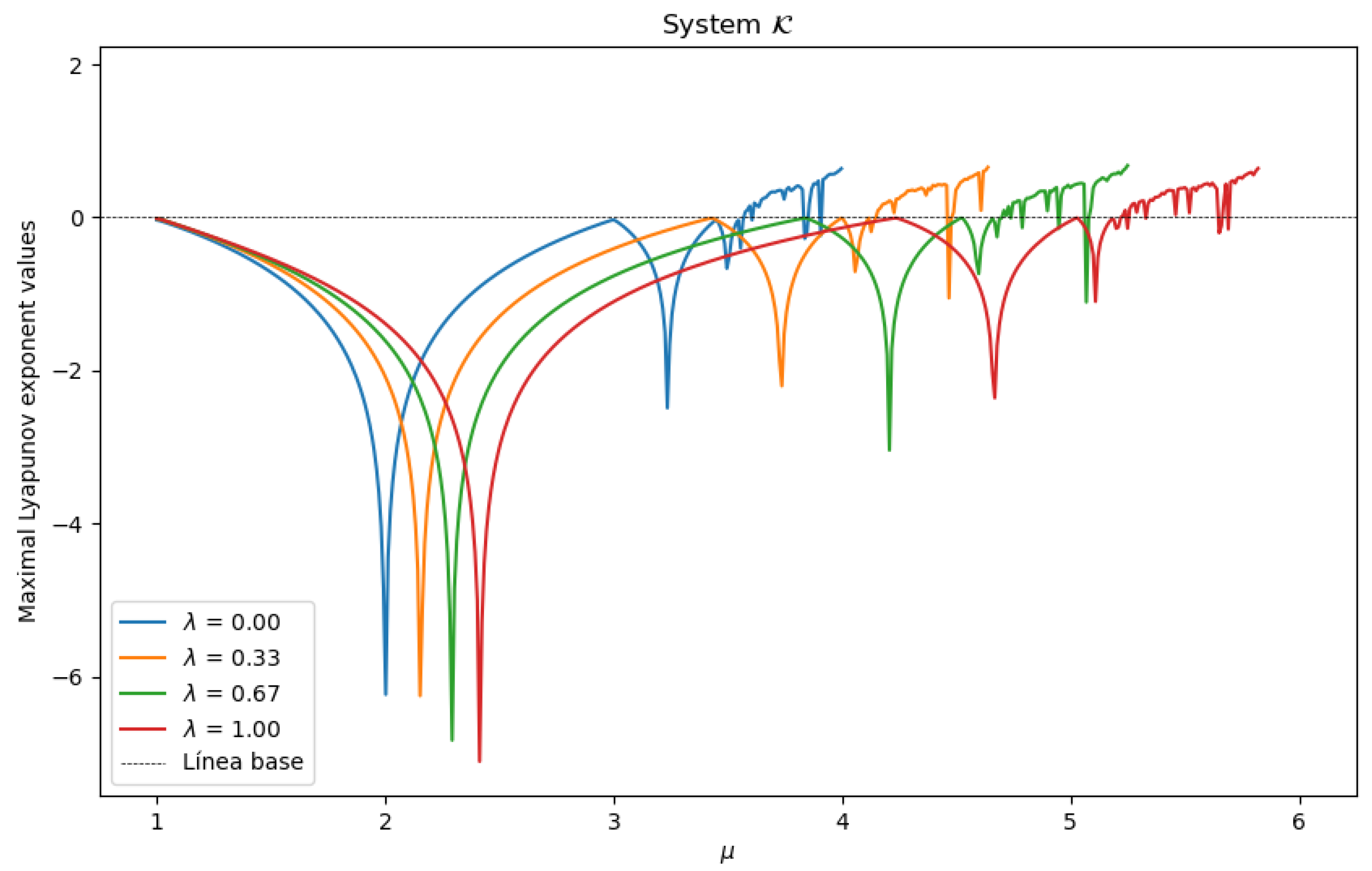
The following Figure 12 presents the graphs associated with this exponent, where a graph of the maximum Lyapunov exponent for each value of $\lambda$ was first considered.

Placing the previous graphs together gives us a different perspective of the results obtained, as shown below.

From Figure 13, we can say that there are points where chaotic behavior is present for each value of $\lambda$. On the other hand, it should be noted that although different systems began to have chaotic behavior, this does not mean that they cannot become stable again.

Another point that draws attention is the behavior of the system when it reaches 0. When the system goes through a peak of stability, it grows rapidly until it reaches 0, but it does not exceed it and has another peak of stability. This behavior is repeated several times before reaching a behavior that is highly sensitive to the initial conditions.

The above motivates us to compare this analysis with that of the bifurcation diagram since conclusions were previously obtained regarding when the system stops being stable for a fixed point. It was observed that stability can be preserved by means of a periodic orbit, so it is interesting to observe what coincidence we could find around the points where the maximum Lyapunov exponent is 0.

As with the bifurcation diagram, it can also be highlighted that the graphical behaviors were similar for different values of $\lambda ,$ and the main difference was seen as a translation between one system and another, that is, there would be a phase change between systems.

7. Bifurcation Points

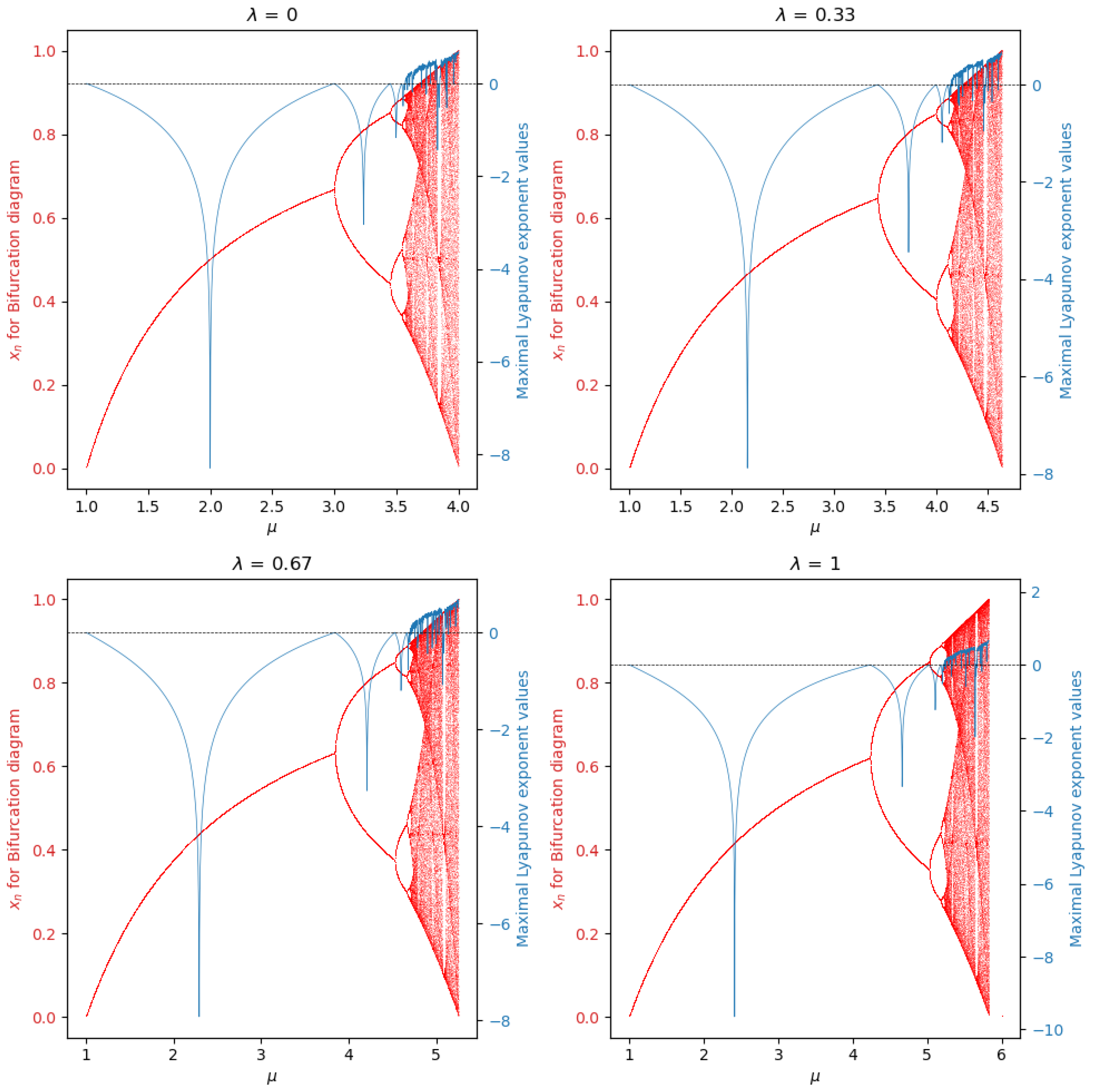
Given the similarity between the last two graphical results, the idea arises to overlap the bifurcation diagram on the diagram of the maximal Lyapunov exponent and see what can be obtained. In this section, we will estimate the first bifurcation points for the values of $\lambda$ already discussed in the previous sections.

Observing both of the overlapped diagrams in Figure 14, it can be seen that the values of $\mu$ in which the maximal Lyapunov exponent was equal to 0 coincide with the points where bifurcations were generated. Therefore, we can look for these bifurcation points to know the transition spaces between types of behaviors.

We also observed that these behavioral changes can range from stable to stable periodic behavior, as well as from stable periodic to chaotic behavior.

First, we set a value of $\lambda$. Then, following an iterative process, we found the transition values in terms of $\mu$ looking at the changes in the sign in the maximum Lyapunov exponent, whose distance between its corresponding maximal Lyapunov exponent and 0 was the smallest one. To compute these numerical approximations, we used Python 3.11.9 with its matplotlib.pyplot 3.5.3 and numpy 2.0 libraries, and we achieved this by considering a neighborhood close to the value 0 for the maximum Lyapunov exponent and setting a length of 10,000 elements within that interval. At that point, we computed the minimum distance between the value of the maximum Lyapunov exponent and 0. That value will then be an approximation of the value of $\mu$, where the maximum Lyapunov exponent is very close to 0.

Then, we determined the following regions in terms of their dynamic behavior.

(a)

$\lambda =0$, then $\mathcal{K}\left(x_n\right)=\mu x_n(1-x_n)$, and the bifurcation points $\mu$ are as follows:

–

From stable to period 2: $\mu \approx 3$;

–

From period 2 to period 4: $\mu \approx 3.45$;

–

From period 4 to chaos: $\mu \approx 3.56$.

(b)

$\lambda =0.33$, then ${\displaystyle \mathcal{K}\left(x_n\right)=\frac{\mu x_n(1-x_n)}{1+0.33x_n}}$, and the bifurcation points $\mu$ are as follows:

–

From stable to period 2: $\mu \approx 3.43$;

–

From period 2 to period 4: $\mu \approx 3.99$;

–

From period 4 to chaos: $\mu \approx 4.14$.

(b)

$\lambda =0.67$, then ${\displaystyle \mathcal{K}\left(x_n\right)=\frac{\mu x_n(1-x_n)}{1+0.67x_n}}$, and the bifurcation points $\mu$ are as follows:

–

From stable of period 2: $\mu \approx 3.84$;

–

From period 2 to period 4: $\mu \approx 4.53$;

–

From period 4 to chaos: $\mu \approx 4.70$.

(b)

$\lambda =1$, then $\mathcal{K}\left(x_n\right)={\displaystyle \frac{\mu x_n(1-x_n)}{1+x_n}}$, and the bifurcation points $\mu$ are as follows:

–

From stable to period 2: $\mu \approx 4.23$;

–

From period 2 to period 4: $\mu \approx 5.03$;

–

From period 4 to chaos: $\mu \approx 5.22.$

Figure 15 shows the previous graph where vertical lines were drawn that coincide with the values of $\mu$ previously calculated for each graph.

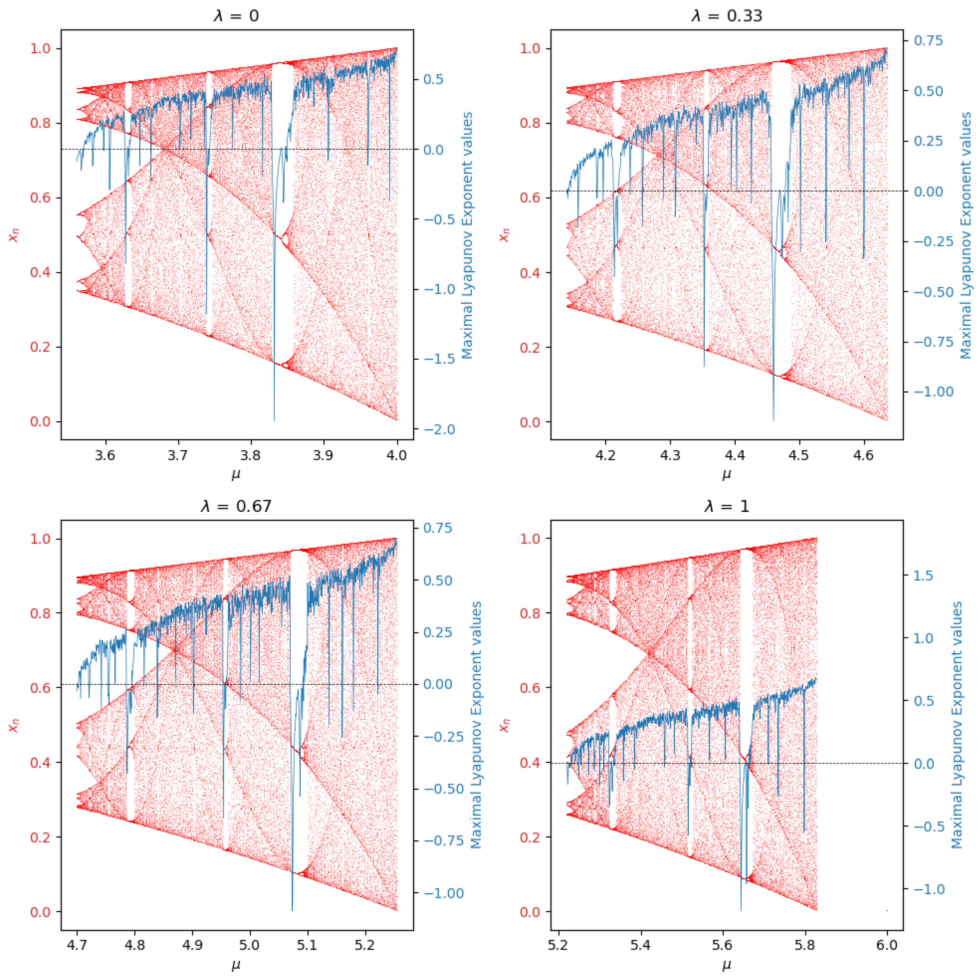
Next, Figure 16 shows the same graph overlapped before but emphasizes the chaotic part of each system associated with a value of $\lambda$.

These last pictures confirm what has been studied: the non-chaotic parts of the bifurcation diagram directly coincide with the values of the maximal Lyapunov exponent that define behaviors with low sensitivity to initial conditions. Moreover, the distance between bifurcation points increases as $\lambda$ increases.

8. Conclusions

In this paper, we investigated the dynamics of the discrete dynamical system given by (2), which provides a unified class of one-dimensional discrete maps that contains the logistic map as a particular case. Using analytic and graphical methods, we illustrated the influence of parameters $\mu$ and $\lambda$ in the system’s stability, periodicity, and chaotic behavior. In addition, the overlapping of bifurcation diagrams with a maximal Lyapunov exponent plots shows the precise bifurcation points of this discrete dynamical system.

Adding the parameter $\lambda$ enhances the flexibility of the discrete logistic map for modeling purposes. This opens new opportunities for multidisciplinary applications such as population dynamics or encryption algorithms, where the logistic map has provided outstanding profits. In addition, it also opens the opportunity to study questions of mathematical nature, such as the extension to higher dimensions, the study of fractional and memory-dependent systems [4,19,20], stochastic perturbations [21], or encryption applications [22].