1. Introduction
Quantile-based inference has long been a topic of interest in risk evaluation in the financial industry and other contexts. Notable applications include the following: the widely used risk measure value at risk (VaR), which corresponds directly to a quantile; coherent risk measures, which are often derived from quantile transformations; and quantile regression, which has been employed as a tool for making portfolio investment decisions.
For a continuous random variable
X with a cumulative distribution function (CDF)
density function
, and
the
p-th quantile is defined as
Given a sample
from
the simplest estimator of
is the sample quantile. Under mild conditions, it is asymptotically normal, but its asymptotic variance
is large, particularly in the tails. Hence, it behaves poorly for small sample sizes, and alternative estimators are needed. An obvious choice is the kernel quantile estimator
where
is the inverse of the empirical distribution function,
is a suitably chosen kernel, and
is a bandwidth. Conditions on the bandwidth and the kernel must be imposed to ensure consistency, asymptotic normality, and the higher-order accuracy of
Quantile-based inference has also been of significant interest to the authors of this paper. We derived in [
1] a higher-order expansion for the standardized kernel quantile estimator, thus extending the long-standing flagship results obtained in [
2,
3]. Our expansion was non-trivial, because the influence of the bandwidth made the balance between bias and variance delicate.
In [
4], we derived an Edgeworth expansion for the studentized version of the kernel quantile estimator, where the variance of the estimator was estimated using the jackknife method. This result is particularly important for practical applications, as the variance is rarely known in real-world scenarios. By inverting the Edgeworth expansion, we achieved a uniform improvement in coverage accuracy compared to the inversion of the asymptotically normal approximation. Our results are applicable in improving the inference for quantiles when the sample sizes are small-to-moderate. This situation often occurs in practice. For example, if monthly loss data are used in risk analysis, then the accumulated data for 10 years amounts to 120 observations. Another example is that of the daily data gathered from the stock market, which has approximately 250 active trading days each year.
The global financial crisis (GFC) from mid-2007 to early 2009 had a profound effect on many banks around the world. There were numerous reasons for the crisis; however, in mathematical terms, one important reason was that the banks’ risk estimates based on the widespread measure value at risk (VaR) happened to be very inaccurate. The key shortcomings of VaR are that it assumes normal market conditions, tends to ignore the tail risk, and shows a tendency to reduce risk estimates during calm periods (encouraging leverage) and increase them during volatile periods (forcing deleveraging). These limitations were seriously scrutinized after the GFC, with bank regulators proposing alternative risk measures. As a result, the seminal paper of Newey and Powell [
5] introducing expectiles was rediscovered, and many advantageous properties of expectiles were noted and extended.
The coherency requirement for a risk measure in finance was first formulated in the seminal paper by [
6] and has been widely used since then. We note that VaR is not a coherent risk measure, mainly because it does not satisfy the subadditivity property. The average value at risk (AVaR) does satisfy the subadditivity property and turns out to be a coherent risk measure. It was considered around 2009 as an alternative risk measure by the Basel Committee of Banking Supervision. Meanwhile, academic research on the properties of risk measures continued. The elicitability property was pointed out as another essential requirement in [
7]. The latter property is an important requirement associated with effective backtesting. It then turned out that expectiles “have it all”, as they are simultaneously coherent and elicitable. Moreover, it has been shown (for example, in [
8]) that expectiles are the only law-invariant risk measures that are simultaneously coherent and elicitable. Furthermore, ref. [
9] noted that another desirable property, the isotonicity with respect to the usual stochastic order, also holds.
Due to the above properties, expectiles became widely adopted in risk management after the GFC. The asymptotic properties of expectile regression estimators and test statistics were investigated more deeply following the paper by [
5]. Asymptotic properties of the
sample expectiles, such as uniform consistency and asymptotic normality, were shown under weak assumptions, and a central limit theorem for the expectile process was proven in [
10]. Expectile estimators for heavy-tailed distributions were also investigated in the same paper. Under strict stationarity assumptions, the authors in [
11] showed several first-order asymptotic properties, such as consistency, asymptotic normality, and qualitative robustness. In [
12], the authors compared the merits of estimators in the quantile regression and expectile regression models.
Less attention has been paid in the literature to confidence interval construction, with the only exception, to our knowledge, being the paper by [
13]. Again, these intervals are constructed based on first-order asymptotics using asymptotic normality.
From a practical point of view, ref. [
14] is a review paper which discusses known properties of expectiles and their financial meaning, and which presents real-data examples. The paper also refines some of the results in [
15]. Another similar review discussing the regulatory implementation of expectiles is [
16].
While first-order asymptotic inference results for expectiles are well established, developing higher-order asymptotics is more challenging.
It was natural for us, therefore, to turn to expectiles and to propose methods for improved inference about expectiles for small-to-moderate sample sizes. The methodology to achieve this goal is to derive the higher-order Edgeworth expansion for both the standardized and studentized versions of the kernel-based estimator of the expectile. By inverting the expansion, we can construct improved confidence intervals for the expectile. This article suggests this methodology and illustrates its effectiveness. The article is organized as follows. In
Section 2, we introduce some notations, definitions, and auxiliary statements needed in the subsequent sections.
Section 3 presents our main results about the Edgeworth expansion of the asymptotic distribution of the estimator. This section is subdivided into three subsections. The first subsection deals with the
standardized kernel-based expectile estimator. The second subsection discusses the related results for the
studentized kernel-based expectile estimator. Whilst the first subsection is mainly of theoretical interest, the results of the second subsection can be directly applied to derive more accurate confidence intervals for the expectile of the population for small-to-moderate samples. The third subsection discusses a Cornish–Fisher-type approximation for the quantile of the kernel-based expectile estimator. The application for accurate confidence interval construction presents the main purpose of our methodology. Its efficiency is illustrated numerically in
Section 4.
Section 5 summarizes our findings. The technical results and proofs of the main statements of the paper are postponed to
Appendix A.
2. Materials and Methods
From a methodological standpoint,
is an
L-estimator: it can be written as a weighted sum of the order statistics
Consider a random variable
Using the notations
Newey and Powel introduced in [
5] the expectile
as the minimizer of the asymmetric quadratic loss,
and we realize that its empirical variant can also be represented as an
L-statistic. When
we obtain
, which means that the expectiles can be interpreted as an asymmetric generalization of the mean. In addition, it has been shown in several papers (see, for example, [
14]) that the so-called expectile-VaR (
is a coherent risk measure when
, as it satisfies the four coherency axioms from [
6]. Any value of
can be used in the definition of the expectile but, for the reason mentioned in the previous sentence, we will assume that
in the theoretical developments of this paper.
The asymptotic properties of
L-statistics are usually discussed by first decomposing them into a
U-statistic plus a small-order remainder term and then applying the asymptotic theory of the
U-statistic. Initially, the
L statistic is written as
, where
is the empirical distribution function and the
score function does not involve
For the presentation (
2), however, such a decomposition is impossible as the “score function” becomes a delta function in the limit. Therefore, a novel dedicated approach is needed. In the case of quantiles, details about such an approach are given in [
4]. Our current paper shows how the issue can also be resolved in the case of expectiles. The main tools in our derivations are some large deviation results on
U-statistics from [
17] and standard asymptotic results from [
18].
Remark 1. We mention, in passing, that in the paper by [19] it is shown that expectiles of a distribution F are in a one-to-one correspondence to quantiles of another distribution G that is related to F by an explicit formula. It was tempting to use this relation to utilize our results from [4] for constructing confidence intervals for the expectiles of F. We examined this option and realized that the correspondence is quite complicated, involving functionals of F that need to be estimated by the data. Our conclusion was that proceeding this way was not an option for constructing precise confidence intervals for the expectiles. Hence, our way to proceed is to deal directly from the very beginning with the definition of the expectile of We start with some initial notations, definitions, and auxiliary statements.
We consider a sample of n independently and identically distributed random variables with density and cumulative distribution functions respectively.
Let us define
where
is an indicator function. Looking at the original definition (
3), we can define the (true theoretical) expectile
as a solution to the equation
Using the relation
, we realize that the defining Equation (
4) leads to the same solution as the defining Equation (2) in [
14] or the defining Equation (2) in [
10].
As discussed in [
10], the
-expectile
satisfies the Equation
Using integration by parts, we have the following proposition:
Proposition 1. Assume that . Then, we havewhere and Thus, an estimator of the expectile is given by a solution of the equationwhere is the sample mean and is the empirical distribution function. Holzmann and Klar in [
10] showed the uniform consistency and asymptotic normality of
. In this paper, we study the higher-order asymptotic properties of the expectile estimator. To study the higher-order asymptotics, we use a kernel-type estimator
of the distribution function
, instead of
.
Let us define kernel estimators of the density and distribution function:
where
is a kernel function and
is an integral of
. We assume that
and
Here,
h is a bandwidth where
. Hereafter, we assume that the bandwidth
.
As in the case of quantile estimation, we are using a kernel-smoothed estimator of the cumulative distribution function in the construction of the expectile estimator. The reason for switching to the kernel-smoothed version of the empirical distribution function in the definition of our expectile estimator is that only for this version is it possible to show the
validity of the Edgeworth expansion. As discussed in detail in [
4], if we use a kernel estimator with an informed choice of bandwidth and a suitable kernel then the resulting expectile estimator can be easily studentized; the Edgeworth expansion up to order
for the studentized version will be derived and the theoretical quantities involved in the expansion can be shown to be easily estimated. In addition, a Cornish–Fisher inversion can be used to construct confidence intervals for the expectile (which is the main goal of the inference in this paper). The resulting confidence intervals are more precise than the intervals obtained via inversion of the normal approximation and can be used to improve the coverage accuracy for moderate sample sizes.
Hence, from now on we will discuss the higher-order asymptotic properties of the estimator
of
that satisfy
Let us define
Then, similarly to Proposition 1, we have the following Proposition:
Proposition 2. If the kernel function satisfies the condition (a1), the kernel expectile estimator is given by the solution of the equationFor our further discussion, we define the following quantities: Definition 1. Note that holds and that , and denote the biases of the kernel estimators of , and
Using Equations (
6) and (
7), we have
Since we intend to discuss the Edgeworth expansion with a residual term
, we will obtain the asymptotic representation with residual term
, where
as
. When we obtain the Edgeworth expansion until the order
, it follows from Esseen’s smoothing lemma that we can ignore the terms of order
.
Similarly to the
notation, we will also be using the
notation that follows the definition
Note that we can also ignore the terms when we discuss the Edgeworth expansion with residual term .
4. Discussion
Given that the main application domain of expectiles has been risk management, we also want to illustrate the application of our methodology in this area. As discussed in
Section 2,
is a coherent risk measure when
It is easy to check (or compare p. 46 of ([
15])) that
holds. In addition, most interest in risk management is in the tails. If the random variable of interest
X represents an outcome, then
represents a loss, and one would be interested in losses in the tail. To illustrate the effectiveness of our approach for constructing improved confidence intervals, we need to compare simulation outcomes with the population distribution for which the true expectile is known precisely. Such examples are relatively scarce in the literature. Some suitable exceptions are discussed in [
14]. One of these exceptions is the exponential distribution, which we chose for our illustrations below.
Setting
to be standard exponentially distributed, we have for the values of
the relation
where
is the Lambert
function defined implicitly by means of the equation
(and we note that
for
holds). The Formula (
13) for the expectile of the exponential distribution is derived on page 495 in [
14].
We have used a symmetric compactly supported on
kernel
It is said to be of order
m, where
m is the
mth derivative
for some
and
our numerical experiments, we used the classical second-order Epanechnikov kernel,
With it, the factor in the definition of the estimator
becomes
.
There are at least two ways to produce accurate confidence intervals at level
for the expectile when exploiting the Edgeworth expansion of its studentized version. One approach (we call it the
CF method) is based on using the estimated values
and
obtained by using the Formula (
12). Then, the left-and right-hand sides of the
confidence interval for
at given
are obtained as
Another approach (we call it
numerical inversion) is to use numerical root-finder procedures to solve the two equations
and construct the confidence interval as
Here,
These two methods should be asymptotically equivalent but they deliver different intervals for small sample sizes, with the numerical inversion delivering significantly better results, in terms of closeness to the nominal coverage level.
We provide some details about the numerical implementation at the end of
Appendix A.
With the standardized version, we achieved a better approximation and more precise coverage probabilities across very low sample sizes, such as
across a range of
values, such as
and a range of values of
, such as
for the
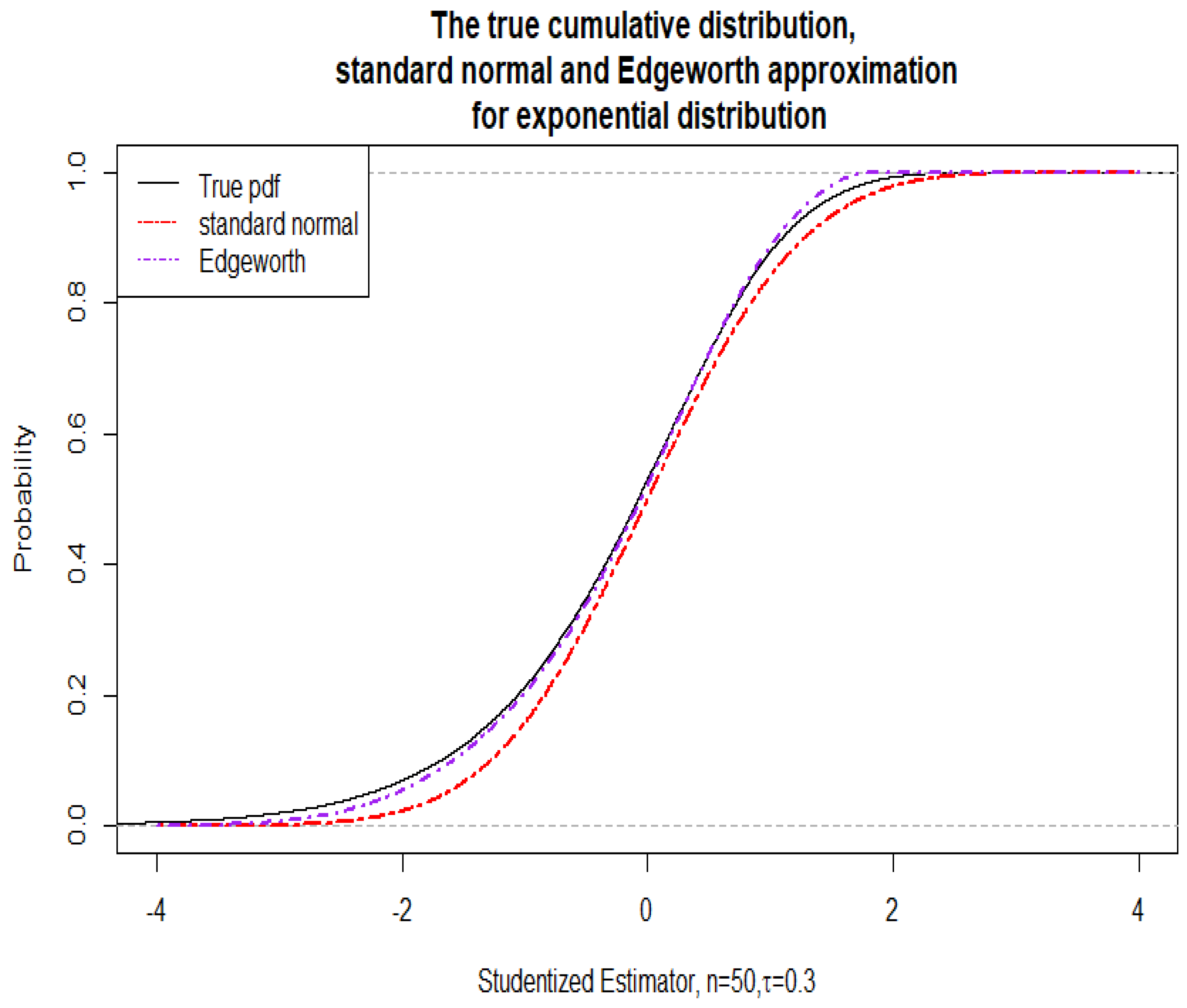
confidence intervals. The approximations were extremely accurate for such small sample sizes. We have not reproduce all these here, as our main goal was to investigate the practically more relevant studentized case. We only include one graph (
Figure 1) where the case
is demonstrated graphically. The “true” cdf of the estimator for comparison was obtained via the empirical cdf based on 50,000 simulations from standard exponentially distributed data of size
The resulting confidence intervals at a nominal
level had actual coverage of 0.90 for the Edgeworth and 0.9014 for the normal approximation. At nominal
, they were 0.9490 and 0.9453, respectively. At nominal
they were 0.9858 for Edgeworth versus 0.9804 for the normal approximation.
In the practically relevant studentized case, we were unable to obtain such good results for sample sizes as low as the ones from the standardized case. This is, of course, to be expected, as in this case there was a need to estimate the and the C quantities using the data. The moderate sample sizes at which the CF and numerical inversion methods deliver significantly more precise results depend, of course, on the distribution of C itself. For the exponential distribution, these turn out to be in the range of 20, 50, 100, 150 to about 200. For larger sample sizes, all three methods—the normal theory-based confidence intervals, the ones obtained by the numerical inversion and the CF-based intervals—become very accurate but the discrepancy between their accuracy becomes negligibly small and, for that reason, we do not report it here.
Before presenting thorough numerical simulations, we include one illustrative graph (
Figure 2) for the case
where the studentized case is demonstrated. The graph demonstrates the virtually uniform improvement when the Edgeworth approximation is used instead of the simple normal approximation. A comparison was made with the “true” cdf (obtained via the empirical cdf based on 50,000 simulations from standard exponentially distributed data of size
). We found that at 50,000 replications a stabilization occurred and that further increase of the replications seemed unnecessary. The resulting confidence intervals at a nominal
level had actual coverage of 0.877 for the numerical inversion of the Edgeworth, with 0.869 for the normal approximation. At
nominal level, the actual coverage was 0.921 for the numerical inversion of the Edgeworth versus 0.917 for the normal approximation.
Next, we include
Table 1 and
Table 2 showing the effects of applying our methodology for constructing confidence intervals for the expectiles. The moderate samples included in the comparison were chosen as 20, 50, 100, 150, and 200. The two tables illustrate the results for two common confidence levels used in practice (
for
Table 1 and
for
Table 2). The best performer in each row is in bold font. Examination of
Table 1 and
Table 2 shows that the “true” coverage probabilities approached the nominal probabilities when the sample size increased. As expected, the discrepancies in accuracy between the different approximations also decreased when the sample size
n increased. As the confidence intervals were based on asymptotic arguments, this demonstrates the consistency of our procedure. For the chosen levels of confidence, our new confidence intervals virtually
always outperformed the ones based on the normal approximation. There appears to be a downward bias in the coverage probabilities across the tables for both normal and Edgeworth-based methods. This bias grows smaller as
n increases above 200. We observe that the value of
also influenced the bias, with smaller values of
impacting the bias more significantly. This was expected, as these values of
lead to expectiles that are further in the right tail of the distribution of the loss variable
X and, hence, are more difficult to estimate. As is known, the Edgeworth approximation’s strength is in the central part of the distribution. However, at small values of
we focus on the tail, where it does not necessarily improve over the normal approximation.


