On the Existence and Uniqueness of Solutions for Neutral-Type Caputo Fractional Differential Equations with Iterated Delays: Hyers–Ulam–Mittag–Leffler Stability

Abstract

This study investigates nonlinear Caputo-type fractional differential equations with iterated delays, focusing on the neutral type. Initially formulated by D. Bainov and the second author of the current paper between 1972 and 1978, these superneutral equations have been extensively studied in scholarly inquiry. The present research seeks to reinvigorate interest in such delays within sophisticated frameworks of differential equations, particularly those involving fractional calculus. The primary objectives are to thoroughly examine neutral-type fractional differential equations with iterated delays and provide novel insights into their existence and uniqueness by applying Bielecki’s and Chebyshev’s norms for solution constraints analysis. Additionally, this work establishes Hyers–Ulam–Mittag–Leffler stability for these equations.

1. Introduction

Fractional differential equations with intricate dependencies of the delay on the solution and its derivatives have been encountered in various domains of science and engineering, showcasing the complexity and depth of mathematical modeling in these fields. Delays have been shown to significantly influence system dynamics, adding analytical layers. A wealth of knowledge has been provided by [1,2], shedding light on fractional calculus intricacies. Functional differential equations with retarded arguments discussed by [3,4] offer broader perspectives on diverse applications.

Recent advancements in fractional calculus have been recognized as expanding its applications across various fields, making it pertinent for superneutral equations with iterated delays to be revisited. These equations are deemed critical for modeling systems with long memory effects, such as those found in biological systems, engineering (e.g., lossless transmission lines), vibrating masses, and physics [1,4,5,6,7,8]. The growing interest is driven by their potential to provide more accurate predictions compared to traditional models. Essential groundwork has been laid by our findings for numerous numerical studies focused on real-world applications such as control system optimization or population dynamics modeling—areas where precise solutions are crucial. Foundational insights into uniqueness and stability analysis have been provided, enabling further exploration into practical implementations using computational simulations akin to those developed previously.

Numerous studies have been dedicated to exploring the existence and uniqueness of solutions to initial problems related to differential functional equations. The most comprehensive findings regarding differential functional equations in a Banach space often stem from utilizing the principle of fixed points for contraction operators. Nonetheless, researchers are intrigued by uncovering the specific conditions that govern the existence and uniqueness of solutions for particular classes of differential functional equations situated in finite-dimensional and countable-dimensional spaces.

Functional differential equations of superneutral type represent a variant of neutral-type differential functional equations, where the transformed argument intricately intertwines with the derivative of the solution. Reference [9] has rigorously established theorems concerning the local and global existence as well as uniqueness of solutions for differential functional equations of superneutral type with an iterated transformed argument. Noteworthy is the imposition of Lipschitz conditions on the right-hand sides of the equations in the theorems pertaining to the global existence of solutions within the realm of vector functions showcasing derivatives that adhere to the Lipschitz condition. These types of iterated arguments have been connected to foundational studies on difference-differential equations. The work [10] has addressed scalar linear differential-difference equations of neutral type for smooth solutions over extended intervals. The paper [11] has used polynomial quasi-solutions to ensure smoothness at delay-multiple points by compensating dimensional inaccuracies through residuals. Iterative functional differential equations have been further discussed in the works [12,13,14,15], providing existence results for smooth and analytical solutions.

In the realm of mathematical research, related to the current work, ref. [16,17,18,19] stand out as pivotal references, delving into the nuanced aspects of existence and uniqueness concerning solutions to the Caputo fractional-order delay differential equations. Employing advanced mathematical tools such as Chebyshev and Bielecki norms alongside the Banach contraction principle, the authors of the aforementioned works have established the existence, uniqueness, and Ulam–Hyers–Mittag–Leffler stability of solutions to the Caputo fractional-order delay differential equation. This groundbreaking research underscores the growing significance and widespread applications of stability analysis in various forms of fractional differential equations, reflecting the evolving landscape of scientific inquiry and technological innovation, as well as the importance of the integral representation of the solution when studying different types of stability [20,21]. Alternative approaches through the integral representation of solutions [22] and the quantum Laplace transform [23] have been acknowledged to provide sufficient conditions for Hyers–Ulam type stability, suggesting these methods can be utilized instead of the classical fixed-point approach.

Significant developments have deepened our understanding of stability within fractional systems. In [24], Ulam stabilities for nonlinear iterative integro-differential equations are explored, while [25] examines asymptotic properties specific to fractional delay systems. The work in [26] delves into Riemann–Liouville order stability concepts. Additionally, Ulam stability is investigated across varied contexts in [27], whereas Hyers–Ulam–Rassias considerations are detailed for first-order cases in [28]. Contributions further elucidate Hyers–Ulam–Rassias frameworks concerning linear fractional systems under distributed delays involving Riemann–Liouville derivatives [22].

Despite extensive literature on the existence, uniqueness, and stability of delay fractional differential equations, there remains a noticeable gap in addressing iterated delays ($\mathcal{ID}$) within the current body of research. This is an area that has yet to be fully explored.

Consider the following initial value problem ($\mathcal{IVP}$) for the Caputo fractional differential equation of neutral-type ($\mathcal{NF}rDE$) with $\mathcal{ID}$:

$$\begin{array}{cc}\hfill & D^{\alpha }x\left(t\right)=f\left(t,x\left(t\right),D^{\alpha }x\left(t\right),x\left({\tau }_0\right),D^{\alpha }x\left({\tau }_0\right)\right),t\in J_1\hfill \\ \hfill & x\left(t\right)=0,t\in J_0,\hfill \end{array}$$

(1)

where

$$\begin{array}{cc}\hfill {\tau }_k& ={\tau }_k\left(t,x\left(t\right),D^{\alpha }x\left(t\right),x\left({\tau }_{k+1}\right),D^{\alpha }x\left({\tau }_{k+1}\right)\right),k=0,1,\dots ,m-1\hfill \\ \hfill {\tau }_m& ={\tau }_m\left(t,x\left(t\right),D^{\alpha }x\left(t\right)\right),\hfill \end{array}$$

(2)

and $x\in \mathbb{R},$ and $D^{\alpha }$ is the Caputo-type fractional derivative of order $0<\alpha <1$ with the lower limit zero and $t\in J,$ where $J=J_0\bigcup J_1,$$J_0=(-\infty ,0],J_1=(0,1].$

Let denote by $C(J,\mathbb{R})$ the Banach space of continuous functions $J\to \mathbb{R}$ with topology of uniform convergence, and let $F\in C(J,\mathbb{R})$ be a bounded function,

$${\Omega }_s=\{\xi :\left|\xi \right|\le {\omega }_s,{\omega }_s\in \mathbb{R}\}$$

$${\omega }_0={\displaystyle \frac{1}{\Gamma \left(\alpha \right)}}\underset{0}{\overset{1}{\int }}{(t-s)}^{\alpha -1}F\left(s\right)\mathrm{d}s,{\omega }_1=sup\{F\left(t\right),t\in J\}.$$

Finally, we consider D as a subset of $J\times G,G=G_1\times G_1,G_1={\Omega }_0\times {\Omega }_1.$

Remark 1. 

As detailed in [29], when tackling these specific equations, it is beneficial to assume that both the solution and its fractional derivative maintain Lipschitz continuity. This assumption plays a crucial role in ensuring the existence and uniqueness of the solutions. To confirm these properties, all functions involved must exhibit Lipschitz continuity across their arguments, with corresponding Lipschitz constants meeting predefined constraints.

Let us denote by $C^{*}(J,\mathbb{R})$ the set of Lipshitz continuous functions on the interval J with Caputo-type fractional derivative satisfying the Lipschitz condition as well, i.e., $x\in C^{*}(J,\mathbb{R})$ follows the assumptions

i.

$\left|x\left(\tau \right)-x\left(\tilde{\tau }\right)\right|\le {\delta }_x|\tau -\tilde{\tau }|;$

ii.

$\left|D^{\alpha }x\left(\tau \right)-D^{\alpha }x\left(\tilde{\tau }\right)\right|\le {\delta }_x^{\alpha }|\tau -\tilde{\tau }|.$

The structure of this paper is as follows: Section 2 outlines fundamental concepts and insights into fractional calculus theory. Section 3 presents the main results on the existence and uniqueness of solutions for nonlinear $\mathcal{NF}rDE$ with $\mathcal{ID}$ (1) through Chebyshev and Bielecki norms, alongside results on Ulam–Hyers–Mittag–Leffler stability for the problem addressed. An example provided in Section 4 illustrates the main results. Lastly, Section 5 concludes with research findings and commentary.

2. Fractional Calculus: Definitions

This section presents essential concepts and findings that are utilized in subsequent parts of the paper. We start by detailing definitions from fractional calculus, with references [1,2] offering all necessary features and information on fractional derivatives.

Definition 1. 

Let $a\in \mathbb{R},$$\alpha \in (0,1)$ be arbitrary constants and f be a locally Lebesgue integrable function.

(i) 

The fractional order integral α of a function f with a lower limit of integration a can be determined by the formula

$$I_{a+}^{\alpha }f\left(t\right)={\displaystyle \frac{1}{\Gamma \left(\alpha \right)}}\underset{a}{\overset{t}{\int }}{(t-s)}^{\alpha -1}f\left(s\right)\mathrm{d}s,$$

where $\Gamma$ is the gamma function.

(ii) 

The Riemann–Liouville fractional derivative is given by

$${}_{RL}D_{a+}^{\alpha }f\left(t\right)={\displaystyle \frac{\mathrm{d}}{\mathrm{dt}}}{I}_{a+}^{1-\alpha }f\left(t\right),D_{a+}^{0}f\left(t\right)=f\left(t\right).$$

(iii) 

The Caputo fractional derivative for all $t>a$ of fractional order α is expressed as

$$D_{a+}^{\alpha }f\left(t\right)={}_{RL}D_{a+}^{\alpha }[f\left(s\right)-f\left(a\right)]\left(t\right).$$

If f is absolutely continuous on $\mathbb{R}$, then, the next formula gives a direct definition of the Caputo left-sided derivative:

$$D_{a+}^{\alpha }f\left(t\right)={\displaystyle \frac{1}{\Gamma (1-\alpha )}}\underset{a}{\overset{t}{\int }}{\displaystyle \frac{f^{\prime }\left(s\right)\mathrm{d}s}{{(t-s)}^{\alpha }}}.$$

The following relations [2] containing fractional derivatives and special functions will be used:

(a)

$D_{a+}^{0}f\left(t\right)=f\left(t\right);$

(b)

$D_{a+}^{\alpha }{I}_{a+}^{\alpha }f\left(t\right)=f\left(t\right);$

(c)

$I_{a+}^{\alpha }{D}_{a+}^{\alpha }f\left(t\right)=f\left(t\right)-f\left(a\right);$

(d)

$\Gamma (\alpha +1)=\alpha \Gamma \left(\alpha \right)$ and $\Gamma \left(\alpha \right)\Gamma (1-\alpha )={\displaystyle \frac{\pi }{sin\alpha \pi }}$ (Euler’s reflection formula).

Lemma 1 

([17]). For $\vartheta >0$ and $\gamma >-1,$

$$\underset{0}{\overset{t}{\int }}{(t-s)}^{\vartheta -1}{s}^{\gamma }\mathrm{d}s={\displaystyle \frac{\Gamma \left(\vartheta \right)\Gamma (\gamma +1)}{\Gamma (\vartheta +\gamma +1)}}{t}^{\vartheta +\gamma }.$$

Lemma 2. 

The $\mathcal{IVP}$ for $\mathcal{NF}rDE$ (1) is equivalent to the following integral representation:

$$x\left(t\right)=\left\{\begin{array}{cc}0,\hfill & t\in J_0,\hfill \\ {\displaystyle \frac{1}{\Gamma \left(\alpha \right)}}{\int }_0^t{(t-s)}^{\alpha -1}f\left(s,x\left(s\right),D^{\alpha }x\left(s\right),x\left({\tau }_0\right),D^{\alpha }x\left({\tau }_0\right)\right)ds,\hfill & t\in J_1,\hfill \end{array}\right.$$

(3)

where ${\tau }_k,k=0,1,\dots ,m$ are defined by (2).

Remark 2. 

As highlighted in [9], we assume that restrictions on the growth of the functions f and ${\tau }_k$ in $\mathcal{IVP}$ for $\mathcal{NF}rDE$ (1) are established through Lipschitz conditions for scalar norms in $\mathbb{R}$. Then, the conditions for the solution of the inequality $x\left({\tau }_k\right)⩽{\tau }_k$ can be formulated in terms of quadratic inequalities, independent of m, with respect to the corresponding Lipschitz constants.

The next two sections outline two distinct cases of the main results. The first case employs a uniform Lipschitz constant across all arguments of the functions, facilitating broader applicability in qualitative analysis while potentially sacrificing some specificity. Conversely, the second case assigns distinct Lipschitz constants to each argument in the right side of the equation, thereby enhancing precision in the analysis.

3. Existence and Uniqueness of Solutions: Ulam–Hyers–Mittag–Leffler Stability of the Solutions

3.1. Case 1 of the Main Results: Unified Lipschitz Constants

This section demonstrates results related to the existence and uniqueness of solutions for the $\mathcal{IVP}$ for $\mathcal{NF}rDE$ (1) over interval $J.$ We establish these findings under the following assumptions:

$\left({\aleph }_1\right)$ 

The function f is defined and continuous in the domain $D=J\times G,$ and for $x_1,x_3\in C^{*}(J,{\Omega }_1)$ (or $x_2,x_4\in C^{*}(J,{\Omega }_0)$) satisfies

(a) 

$|f\left(t,x_1,x_2,x_3,x_4\right)|\le F\left(t\right);$

(b) 

$f\left(t,x_1,x_2,x_3,x_4\right)-f\left(t,y_1,y_2,y_3,y_4\right)|\le {\delta }_f{\sum }_{j=1}^4\left|x_j-y_j\right|,$ where ${\delta }_f$ is positive constant;

(c) 

$f\left(0,0,0,0,0\right)=0.$

$\left({\aleph }_2\right)$ 

The functions ${\tau }_k,k=0,1,\dots ,m-1$ are defined and continuous in the domain $D=J\times G,$ and ${\tau }_m:J\times G_1$ and for $x_1,x_3\in C^{*}(J,{\Omega }_1)$ satisfies

(a) 

$|{\tau }_k\left(t,x_1,x_2,x_3,x_4\right)|\le t,k=0,1,\dots ,m-1;$

(b) 

$|{\tau }_m\left(t,x_1,x_2\right)|\le t;$

(c) 

${\tau }_k\left(t,x_1,x_2,x_3,x_4\right)-{\tau }_k\left(t,y_1,y_2,y_3,y_4\right)|\le {\delta }_{\tau }{\sum }_{j=1}^4\left|x_j-y_j\right|,$ where ${\delta }_{\tau }>0;$

(d) 

${\tau }_m\left(t,x_1,x_2\right)-{\tau }_m\left(t,y_1,y_2\right)|\le {\delta }_{\tau }{\sum }_{j=1}^2\left|x_j-y_j\right|$.

$\left({\aleph }_3\right)$ 

The inequality

$$(1+{\displaystyle \frac{1}{\Gamma (\alpha +1)}}){\lambda }_f^{\tau }<1$$

holds for ${\lambda }_f^{\tau }={\delta }_f\left(1+\left({\delta }_{\tau }\left({\delta }_x+{\delta }_x^{\alpha }\right)+1\right){\sum }_{j=0}^m{\left({\delta }_x+{\delta }_x^{\alpha }\right)}^j{\delta }_{\tau }^j\right).$

$\left({\aleph }_4\right)$ 

The inequalities expressed as

$$(1+{\displaystyle \frac{1}{\Gamma \left(\alpha \right)\sqrt{2(2\alpha -1)\theta }}}){\lambda }_f^{\tau }{e}^{\theta }<1\mathrm{for}\mathrm{some}\alpha \in \left({\displaystyle \frac{1}{2}},1\right)\mathrm{and}\theta >0$$

and

$$e^{\theta }(1+{\displaystyle \frac{1}{\Gamma (\alpha +1)}}){\lambda }_f^{\tau }<1\mathrm{for}\mathrm{some}\alpha \in \left(0,1\right)and\theta >0$$

hold for ${\lambda }_f^{\tau }$—defined as in condition $\left({\aleph }_3\right).$

Before presenting our main results, we need the following lemma concerning linear first-order difference inequalities [30,31]:

Lemma 3. 

For the $\mathcal{IVP}$

$$K\left({\xi }_n\right)\le aK\left({\xi }_{n+1}\right)+b,K\left({\xi }_m\right)\le K_m,$$

the inequality

$$K\left({\xi }_0\right)\le a^m{K}_m+b\sum _{j=0}^{m-1}{a}^j$$

holds for $n=0,1,\dots ,m-1,a,b\in \mathbb{R}.$

Proof. 

The proof of the lemma follows immediately by induction, but we may sketch it.

• By simple iteration,

  $$\begin{array}{cc}& K\left({\xi }_{m-1}\right)\le aK\left({\xi }_m\right)+b\le a{K}_m+b\hfill \\ & K\left({\xi }_{m-2}\right)\le aK\left({\xi }_{m-1}\right)+b\le a^2{K}_m+ab+b\hfill \\ & K\left({\xi }_{m-3}\right)\le aK\left({\xi }_{m-2}\right)+b\le a^3{K}_m+a^{2}b+ab+b.\hfill \end{array}$$

  Inductively, it is easy to see that

  $$K\left({\xi }_{m-k}\right)\le a^k{K}_m+b\sum _{j=0}^{k-1}{a}^j.$$

  Assume that the above inequality holds for $k=s,$ i.e., $K\left({\xi }_{m-s}\right)\le a^s{K}_m+b{\sum }_{j=0}^{s-1}{a}^j.$ Then, for $s=0$, we have the initial condition and for $s=1:$ we have $K\left({\xi }_{m-1}\right)\le a{K}_m+b.$ Let $s=s+1;$ we have $K\left({\xi }_{m-(s+1)}\right)\le aK\left({\xi }_{m-(s+1)+1}\right)+b=aK\left({\xi }_{m-s}\right)+b\le a(a^s{K}_m+b{\sum }_{j=0}^{s-1}{a}^j)+b=a^{s+1}{K}_m+b{\sum }_{j=0}^{s-1}{a}^{j+1}+b=a^{s+1}{K}_m+b{\sum }_{j=0}^s{a}^j.$ Thus, for $k=m$ follows our statement. □

Theorem 1. 

Assume that $\left({\aleph }_1\right),\left({\aleph }_2\right)$ are satisfied. Then, the initial problem (1) has at least one solution $x\in C^{*}(J,{\Omega }_1)$. Moreover, if $\left({\aleph }_3\right)$ is satisfied, this solution is unique.

Proof. 

Consider the set $\tilde{X}\subset C^{*}\left(J,{\Omega }_0\right)$ of all functions $\tilde{x}$ satisfying the conditions

$$\begin{array}{cc}\hfill & |\tilde{x}\left(t\right)-\tilde{x}\left(\tilde{t}\right)|⩽{\delta }_x^{\alpha }\left(\right|t-\tilde{t}\left|\right),|x\left(t\right)-x\left(\tilde{t}\right)|⩽{\delta }_x\left(\right|t-\tilde{t}\left|\right),x\left(t\right)=0,t\in J_0,\hfill \end{array}$$

(4)

for $t,\tilde{t}\in J_1;|t-\tilde{t}|⩽h$ where $h>0$ is a sufficiently small number.

Evidently, $\tilde{X}$ is a convex and closed and, according to (4), relatively compact set; then, let the operator ${\mathcal{T}}_f$ act in $\tilde{X}$ consistent with the following formulas:

$$\begin{array}{cc}\hfill {\mathcal{T}}_f\left(\tilde{x}\right)\left(t\right)& =f\left(t,x\left(t\right),\tilde{x}\left(t\right),x\left({\tau }_0\right),\tilde{x}\left({\tau }_0\right)\right),t\in J_1\hfill \\ \hfill {\mathcal{T}}_f\left(\tilde{x}\right)\left(t\right)& =0,t\in J_0\hfill \end{array}$$

(5)

where $x\left(t\right)={\displaystyle \frac{1}{\Gamma \left(\alpha \right)}}{\int }_0^t{(t-s)}^{\alpha -1}\tilde{x}\left(s\right)ds$.

Since $\tilde{x}\left(t\right)=D^{\alpha }x\left(t\right)$, the operator equation $\tilde{x}={\mathcal{T}}_f\left(\tilde{x}\right)$ is equivalent to the initial value problem (1).

It should be established that ${\mathcal{T}}_f$, as defined in (5), acts as a contraction mapping on $\tilde{X}$ with respect to the Chebyshev norm ${\parallel ·\parallel }_C$.

Initially, for $t\in J_0$ and $\tilde{x},\tilde{y}\in \tilde{X}$ by (5),

$$\left|{\mathcal{T}}_f\left(\tilde{x}\right)\left(t\right)-{\mathcal{T}}_f\left(\tilde{y}\right)\left(t\right)\right|=0$$

and for $t\in J_1$, we have

$$\begin{array}{cc}\hfill \left|{\mathcal{T}}_f\left(\tilde{x}\right)\left(t\right)-{\mathcal{T}}_f\left(\tilde{y}\right)\left(t\right)\right|& =|f\left(t,x\left(t\right),\tilde{x}\left(t\right),x\left({\tau }_0\right),\tilde{x}\left({\tau }_0\right)\right)-f\left(t,y\left(t\right),\tilde{y}\left(t\right),y\left({\tau }_0\right),\tilde{y}\left({\tau }_0\right)\right)|,\hfill \end{array}$$

(6)

where ${\tau }_k,k=0,1,\dots ,m$ are given by (2).

Afterward, from assumption $\left({\aleph }_1\right),$ for the right-side part of (6) and $t\in J,k=0,1,\dots ,m$ we have the following inequality:

$$\begin{array}{cc}\hfill & |f\left(t,x\left(t\right),\tilde{x}\left(t\right),x\left({\tau }_0\right),\tilde{x}\left({\tau }_0\right)\right)-f\left(t,y\left(t\right),\tilde{y}\left(t\right),y\left({\tau }_0\right),\tilde{y}\left({\tau }_0\right)\right)|\hfill \\ \hfill & \le {\delta }_f\left(|x\left(t\right)-y\left(t\right)|+|\tilde{x}\left(t\right)-\tilde{y}\left(t\right)|+|x\left({\tau }_0\right)-y\left({\tau }_0\right)|+|\tilde{x}\left({\tau }_0\right)-\tilde{y}\left({\tau }_0\right)|\right).\hfill \end{array}$$

(7)

Now, let us introduce, for clarity, the following notations; as a reminder, each argument ${\tau }_k$ of x and y depends, through iterative steps, on them, i.e.,

$$\begin{array}{cc}& {\tau }_k^x={\tau }_k(t,x\left(t\right),\tilde{x}\left(t\right),x\left({\tau }_{k+1}^x\right),\tilde{x}\left({\tau }_{k+1}^x\right)),k=0,1,\dots ,m-1;\hfill \\ & {\tau }_k^y={\tau }_k(t,y\left(t\right),\tilde{y}\left(t\right),y\left({\tau }_{k+1}^y\right),\tilde{y}\left({\tau }_{k+1}^y\right)),k=0,1,\dots ,m-1;\hfill \\ & {\tau }_m^x={\tau }_m(t,x\left(t\right),\tilde{x}\left(t\right)),{\tau }_m^y={\tau }_m(t,y\left(t\right),\tilde{y}\left(t\right)).\hfill \end{array}$$

Let us first examine the third and fourth addend in the right side of inequality (7) for ${\tau }_k,k=0,1,\dots ,m$ defined by (2), and taking into account that $\tilde{x},\tilde{y}\in \tilde{X}$, it follows that

$$\begin{array}{cc}\hfill |x\left({\tau }_k^x\right)-y\left({\tau }_k^y\right)|& \le \left|x\left({\tau }_k^x\right)-x\left({\tau }_k^y\right)\right|+\left|x\left({\tau }_k^y\right)-y\left({\tau }_k^y\right)\right|\hfill \\ \hfill & \le {\delta }_x\left|{\tau }_k^x-{\tau }_k^y\right|+\left|x\left({\tau }_k^y\right)-y\left({\tau }_k^y\right)\right|\hfill \\ \hfill |\tilde{x}\left({\tau }_k^x\right)-\tilde{y}\left({\tau }_k^y\right)|& \le \left|\tilde{x}\left({\tau }_k^x\right)-\tilde{x}\left({\tau }_k^y\right)\right|+\left|\tilde{x}\left({\tau }_k^y\right)-\tilde{y}\left({\tau }_k^y\right)\right|\hfill \\ \hfill & \le {\delta }_x^{\alpha }\left|{\tau }_k^x-{\tau }_k^y\right|+\left|\tilde{x}\left({\tau }_k^y\right)-\tilde{y}\left({\tau }_k^y\right)\right|.\hfill \end{array}$$

(8)

Note that for the second addend on the right side of (8), we have

$$\underset{0\le {\tau }_k^y\le t}{max}\left|x\left({\tau }_k^y\right)-y\left({\tau }_k^y\right)\right|\le \underset{s\in J}{max}\left|x\left(s\right)-y\left(s\right)\right|=\parallel x-y\parallel ,k=0,1,\dots ,m.$$

Let us introduce the following notations: $\left|x\left(t\right)-y\left(t\right)\right|+\left|\tilde{x}\left(t\right)-\tilde{y}\left(t\right)\right|=U,t\in J_1.$ Now, by assumption $\left({\aleph }_2\right),$ we have, for $k=0,\dots ,m-1$,

$$\begin{array}{cc}\hfill & \left|{\tau }_k^x-{\tau }_k^y\right|=\left|{\tau }_k(t,x\left(t\right),\tilde{x}\left(t\right),x\left({\tau }_{k+1}\right),\tilde{x}\left({\tau }_{k+1}\right))-{\tau }_k(t,y\left(t\right),\tilde{y}\left(t\right),y\left({\tau }_{k+1}\right),\tilde{y}\left({\tau }_{k+1}\right))\right|\hfill \\ \hfill & \le {\delta }_{\tau }\left(\left|x\left(t\right)-y\left(t\right)\right|+\left|\tilde{x}\left(t\right)-\tilde{y}\left(t\right)\right|+\left|x\left({\tau }_{k+1}\right)-y\left({\tau }_{k+1}\right)\right|+\left|\tilde{x}\left({\tau }_{k+1}\right)-\tilde{y}\left({\tau }_{k+1}\right)\right|\right)\hfill \\ \hfill & ={\delta }_{\tau }\left(U+\left|x\left({\tau }_{k+1}\right)-y\left({\tau }_{k+1}\right)\right|+\left|\tilde{x}\left({\tau }_{k+1}\right)-\tilde{y}\left({\tau }_{k+1}\right)\right|\right).\hfill \end{array}$$

(9)

The last two summation terms can be evaluated via (8), as, for $k=m,$ by $\left({\aleph }_2\right),$ we have

$$\begin{array}{cc}\hfill \left|{\tau }_m^x-{\tau }_m^y\right|& =\left|{\tau }_m(t,x\left(t\right),\tilde{x}\left(t\right))-{\tau }_m(t,y\left(t\right),\tilde{y}\left(t\right))\right|\hfill \\ \hfill & \le {\delta }_{\tau }\left(\left|x\left(t\right)-y\left(t\right)\right|+\left|\tilde{x}\left(t\right)-\tilde{y}\left(t\right)\right|\right)={\delta }_{\tau }U.\hfill \end{array}$$

(10)

Let this be denoted by $K\left({\tau }_0\right)=\left|x\left({\tau }_0^x\right)-y\left({\tau }_0^y\right)\right|+\left|\tilde{x}\left({\tau }_0^x\right)-\tilde{y}\left({\tau }_0^y\right)\right|.$ Then, we obtain, for (7),

$$\left|{\mathcal{T}}_f\left(\tilde{x}\right)\left(t\right)-{\mathcal{T}}_f\left(\tilde{y}\right)\left(t\right)\right|\le {\delta }_f(U+K\left({\tau }_0\right)).$$

(11)

Taking into account (8)–(10), for the second addend in the right side of inequality (11), we have

$$\begin{array}{cc}\hfill K\left({\tau }_0\right)& =\left|x\left({\tau }_0^x\right)-x\left({\tau }_0^y\right)+x\left({\tau }_0^y\right)-y\left({\tau }_0^y\right)\right|+\left|\tilde{x}\left({\tau }_0^x\right)-\tilde{x}\left({\tau }_0^y\right)+\tilde{x}\left({\tau }_0^y\right)-\tilde{y}\left({\tau }_0^y\right)\right|\hfill \\ & \le U+\left({\delta }_x+{\delta }_x^{\alpha }\right)|{\tau }_0^x-{\tau }_0^y|\le U\left(1+{\delta }_{\tau }\left({\delta }_x+{\delta }_x^{\alpha }\right)\right)+{\delta }_{\tau }\left({\delta }_x+{\delta }_x^{\alpha }\right)K\left({\tau }_1\right)\hfill \\ \hfill K\left({\tau }_1\right)& =\left|x\left({\tau }_1^x\right)-y\left({\tau }_1^y\right)\right|+\left|\tilde{x}\left({\tau }_1^x\right)-\tilde{y}\left({\tau }_1^y\right)\right|\hfill \\ & \le U\left(1+{\delta }_{\tau }\left({\delta }_x+{\delta }_x^{\alpha }\right)\right)+{\delta }_{\tau }\left({\delta }_x+{\delta }_x^{\alpha }\right)K\left({\tau }_2\right)\hfill \\ & \dots \hfill \\ & K\left({\tau }_{m-1}\right)\le U\left(1+{\delta }_{\tau }\left({\delta }_x+{\delta }_x^{\alpha }\right)\right)+{\delta }_{\tau }\left({\delta }_x+{\delta }_x^{\alpha }\right)K\left({\tau }_m\right)\hfill \\ & K\left({\tau }_m\right)\le U\left(1+{\delta }_{\tau }\left({\delta }_x+{\delta }_x^{\alpha }\right)\right)\hfill \end{array}$$

Then, we derive the following difference inequality:

$$\begin{array}{cc}\hfill K\left({\tau }_n\right)& \le U\left(1+{\delta }_{\tau }\left({\delta }_x+{\delta }_x^{\alpha }\right)\right)+{\delta }_{\tau }\left({\delta }_x+{\delta }_x^{\alpha }\right)K\left({\tau }_{n+1}\right),n=0,1,\dots ,m-1\hfill \\ \hfill K\left({\tau }_m\right)& \le U\left(1+{\delta }_{\tau }\left({\delta }_x+{\delta }_x^{\alpha }\right)\right),U=|x\left(t\right)+y\left(t\right)|+|\tilde{x}\left(t\right)+\tilde{y}\left(t\right)|,t\in J_1.\hfill \end{array}$$

In addition, for the second addend in the right side of (11), it can be derived by Lemma 3 for $a={\delta }_{\tau }\left({\delta }_x+{\delta }_x^{\alpha }\right)$ and $b=K_m=U\left(1+{\delta }_{\tau }\left({\delta }_x+{\delta }_x^{\alpha }\right)\right)$:

$$\begin{array}{cc}\hfill K\left({\tau }_0\right)& \le U\left({\delta }_{\tau }\left({\delta }_x+{\delta }_x^{\alpha }\right)+1\right)\sum _{j=0}^m{\left({\delta }_x+{\delta }_x^{\alpha }\right)}^j{\delta }_{\tau }^j.\hfill \end{array}$$

Finally, for (6), we obtain

$$\begin{array}{cc}\hfill & \left|{\mathcal{T}}_f\left(\tilde{x}\right)\left(t\right)-{\mathcal{T}}_f\left(\tilde{y}\right)\left(t\right)\right|=|f\left(s,x\left(s\right),\tilde{x}\left(s\right),x\left({\tau }_0\right),\tilde{x}\left({\tau }_0\right)\right)-f\left(s,y\left(s\right),\tilde{y}\left(s\right),y\left({\tau }_0\right),\tilde{y}\left({\tau }_0\right)\right)|\hfill \\ \hfill & \le {\delta }_f(U+K\left({\tau }_0\right))\le {\delta }_f\left(1+\left({\delta }_{\tau }\left({\delta }_x+{\delta }_x^{\alpha }\right)+1\right)\sum _{j=0}^m{\left({\delta }_x+{\delta }_x^{\alpha }\right)}^j{\delta }_{\tau }^j\right)U.\hfill \end{array}$$

(12)

Then,

$$\begin{array}{cc}\hfill & |{\mathcal{T}}_f\left(\tilde{x}\right)\left(t\right)-{\mathcal{T}}_f\left(\tilde{y}\right)\left(t\right)|\le {\lambda }_f^{\tau }\left(|x\left(t\right)-y\left(t\right)|+|\tilde{x}\left(t\right)-\tilde{y}\left(t\right)|\right)\hfill \\ \hfill & \le {\lambda }_f^{\tau }\left({\displaystyle \frac{1}{\Gamma \left(\alpha \right)}}{\int }_0^t{(t-s)}^{\alpha -1}|\tilde{x}\left(s\right)-\tilde{y}\left(s\right)|ds+|\tilde{x}\left(t\right)-\tilde{y}\left(t\right)|\right)\hfill \\ \hfill & \le {\lambda }_f^{\tau }\left({\displaystyle \frac{1}{\Gamma \left(\alpha \right)}}{\int }_0^t{(t-s)}^{\alpha -1}ds+1\right)\underset{0\le \overline{s}\le t}{max}|\tilde{x}\left(\overline{s}\right)-\tilde{y}\left(\overline{s}\right)|\hfill \\ \hfill & \le {\lambda }_f^{\tau }\left({\displaystyle \frac{1}{\Gamma (\alpha +1)}}+1\right){\parallel \tilde{x}-\tilde{y}\parallel }_C\hfill \end{array}$$

(13)

where ${\lambda }_f^{\tau }={\delta }_f\left(1+\left({\delta }_{\tau }\left({\delta }_x+{\delta }_x^{\alpha }\right)+1\right){\sum }_{j=0}^m{\left({\delta }_x+{\delta }_x^{\alpha }\right)}^j{\delta }_{\tau }^j\right).$

Therefore, based on assumption $\left({\aleph }_3\right)$, ${\mathcal{T}}_f$ is verified as a contraction with respect to the Chebyshev norm ${\parallel ·\parallel }_C$ on $\tilde{X}$. The subsequent part of the proof follows by the Banach contraction principle. □

Following this, Bielecki’s norm ${\parallel ·\parallel }_B\left({\parallel x\parallel }_B:={max}_{t\in J}\left|x\left(t\right)\right|e^{-\theta t},\theta >0,J\subset {\mathbb{R}}_{+}\right)$ is used to derive the above similar results for (1).

Theorem 2. 

Assume that $\left({\aleph }_1\right),\left({\aleph }_2\right)$, and $\left({\aleph }_4\right)$ are satisfied. Then, the initial problem (1) has a unique solution $x\in C^{*}(J,{\Omega }_1)$.

Proof. 

Similarly to the proof in Theorem 1, as discussed in [16,17,18,19], we establish that ${\mathcal{T}}_f$, as previously defined by (5), is a contraction on X via the Bielecki’s norm ${\parallel ·\parallel }_B$. Given the routine nature of the process, we focus only on the primary difference within our proof:

For any given $t\in J$, we have

$$\begin{array}{cc}& \left|{\mathcal{T}}_f\left(\tilde{x}\right)\left(t\right)-{\mathcal{T}}_f\left(\tilde{y}\right)\left(t\right)\right|\le |f\left(t,x\left(t\right),\tilde{x}\left(t\right),x\left({\tau }_0\right),\tilde{x}\left({\tau }_0\right)\right)-f\left(t,y\left(t\right),\tilde{y}\left(t\right),y\left({\tau }_0\right),\tilde{y}\left({\tau }_0\right)\right)|\hfill \\ & \le {\lambda }_f^{\tau }\left({\displaystyle \frac{1}{\Gamma \left(\alpha \right)}}{\int }_0^t{(t-s)}^{\alpha -1}\underset{0\le s\le t}{max}|\tilde{x}\left(s\right)-\tilde{x}\left(s\right)|ds+\underset{0\le \overline{s}\le t}{max}|\tilde{x}\left(\overline{s}\right)-\tilde{y}\left(\overline{s}\right)|\right)\hfill \\ & \le \left({\displaystyle \frac{1}{\Gamma (\alpha +1)}}+1\right)e^{\theta }{\lambda }_f^{\tau }{\parallel \tilde{x}-\tilde{y}\parallel }_B,\hfill \end{array}$$

where ${\lambda }_f^{\tau }={\delta }_f\left(1+\left({\delta }_{\tau }\left({\delta }_x+{\delta }_x^{\alpha }\right)+1\right){\sum }_{j=0}^m{\left({\delta }_x+{\delta }_x^{\alpha }\right)}^j{\delta }_{\tau }^j\right).$

In a manner analogous to the proof of Theorem 1, it follows that

$${∥{\mathcal{T}}_f\left(\tilde{x}\right)-{\mathcal{T}}_f\left(\tilde{y}\right)∥}_B\le e^{\theta }{\lambda }_f^{\tau }\left({\displaystyle \frac{1}{\Gamma (\alpha +1)}}+1\right){\parallel x-y\parallel }_B,\tilde{x},\tilde{y}\in C^{*}(J,{\Omega }_0).$$

It should be noted that, for $\alpha \in \left({\displaystyle \frac{1}{2}},1\right)$ and by Hölder’s inequality,

$$\begin{array}{cc}\hfill {\int }_0^t{(t-s)}^{\alpha -1}{e}^{\theta s}ds& \le {\left({\int }_0^t{(t-s)}^{2(\alpha -1)}ds\right)}^{{\displaystyle \frac{1}{2}}}{\left({\int }_0^t{e}^{2\theta s}ds\right)}^{{\displaystyle \frac{1}{2}}}\le {\displaystyle \frac{1}{\sqrt{2\theta }}}{\displaystyle \frac{1}{\sqrt{2\alpha -1}}}{e}^{\theta }.\hfill \end{array}$$

Therefore,

$$\begin{array}{cc}& \left|{\mathcal{T}}_f\left(\tilde{x}\right)\left(t\right)-{\mathcal{T}}_f\left(\tilde{y}\right)\left(t\right)\right|\le |f\left(t,x\left(t\right),\tilde{x}\left(t\right),x\left({\tau }_0\right),\tilde{x}\left({\tau }_0\right)\right)-f\left(t,y\left(t\right),\tilde{y}\left(t\right),y\left({\tau }_0\right),\tilde{y}\left({\tau }_0\right)\right)|ds\hfill \\ & \le {\lambda }_f^{\tau }\left({\displaystyle \frac{1}{\Gamma \left(\alpha \right)}}{\int }_0^t{(t-s)}^{\alpha -1}\underset{0\le s\le t}{max}|\tilde{x}\left(s\right)-\tilde{x}\left(s\right)|ds+\underset{0\le \overline{s}\le t}{max}|\tilde{x}\left(\overline{s}\right)-\tilde{y}\left(\overline{s}\right)|\right)\hfill \\ & ={\lambda }_f^{\tau }\left({\displaystyle \frac{1}{\Gamma \left(\alpha \right)}}{\int }_0^t{(t-s)}^{\alpha -1}{e}^{\theta s}ds+e^{\theta \overline{s}}\right){\parallel \tilde{x}-\tilde{y}\parallel }_B\hfill \\ & \le {\lambda }_f^{\tau }{e}^{\theta }\left(1+{\displaystyle \frac{1}{\Gamma \left(\alpha \right)\sqrt{2(2\alpha -1)\theta }}}\right){\parallel \tilde{x}-\tilde{y}\parallel }_B.\hfill \end{array}$$

Thus, ${\mathcal{T}}_f$ acts as a contraction under Bielecki’s norm ${\parallel ·\parallel }_B$ on X. The remaining proof can be derived from the Banach contraction principle as a result of $\left({\aleph }_4\right)$. □

Remark 3. 

It can be shown that the proofs of Theorems 1 and 2 can be performed by the equivalent integral form of the solutions (Lemma 2), as in [17]. The two approaches are equivalent, with some additional assumptions.

Let the conditions $\left({\mathcal{H}}_1^{*}\right)$$|D^{\alpha }x\left(t\right)|\le {\displaystyle \frac{1}{\Gamma (2-\alpha )}}\left|x\left(t\right)\right|$ and $\parallel x\parallel ={max}_{t\in J}\left|x\left(t\right)\right|+{max}_{t\in J}\left|D^{\alpha }x\left(t\right)\right|$ hold for $t\in J$.

Let $X=\left\{x\in C^{*}(J,{\Omega }_1)\right\}$, and consider the operator ${\mathcal{T}}_f:X\to X$, defined by the formula

$${\mathcal{T}}_{f}x\left(t\right)=\left\{\begin{array}{cc}{\displaystyle \frac{1}{\Gamma \left(\alpha \right)}}{\int }_0^t{(t-s)}^{\alpha -1}f\left(s,x\left(s\right),D^{\alpha }x\left(s\right),x\left({\tau }_0\right),D^{\alpha }x\left({\tau }_0\right)\right)ds,\hfill & t\in J_1\hfill \\ 0,\hfill & t\in J_0,\hfill \end{array}\right.$$

where ${\tau }_k,k=0,1,\dots ,m$ are defined by (2).

Let $x,y\in C(J,{\Omega }_1).$ We must show that ${\mathcal{T}}_f$ is a contraction on $X.$

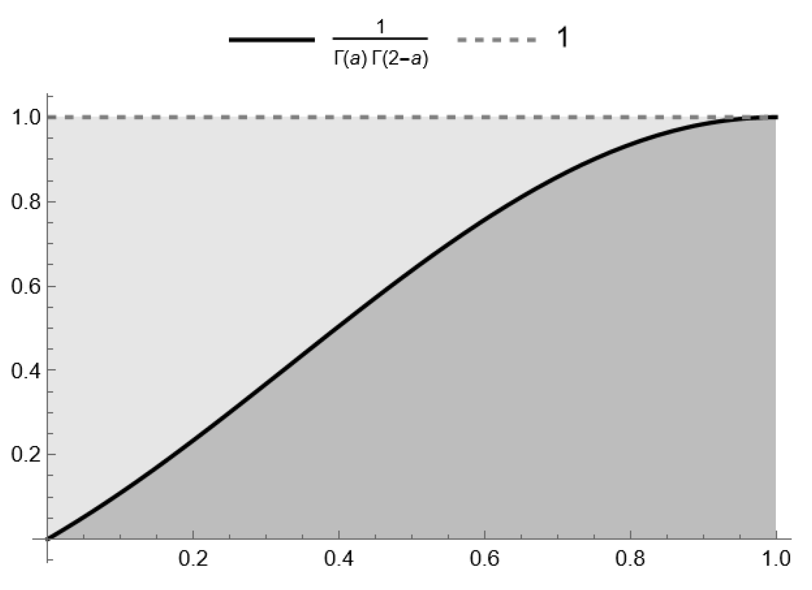
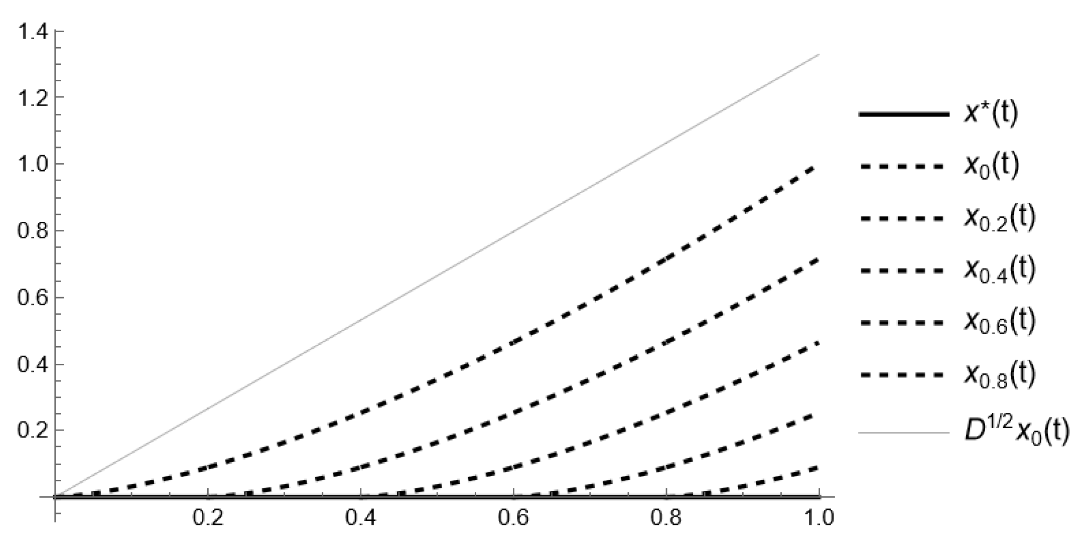
• Obviously, $|{\mathcal{T}}_{f}x\left(t\right)-{\mathcal{T}}_{f}y\left(t\right)|=0,t\in J_0$, and for $t\in J_1$, we have

  $$\begin{array}{cc}& |{\mathcal{T}}_{f}x\left(t\right)-{\mathcal{T}}_{f}y\left(t\right)|⩽{\displaystyle \frac{1}{\Gamma \left(\alpha \right)}}|{\int }_0^t{(t-s)}^{\alpha -1}f\left(s,x\left(s\right),D^{\alpha }x\left(s\right),x\left({\tau }_0\right),D^{\alpha }x\left({\tau }_0\right)\right)ds\hfill \\ & -{\int }_0^t{(t-s)}^{\alpha -1}f\left(s,y\left(s\right),D^{\alpha }y\left(s\right),y\left({\tau }_0\right),D^{\alpha }y\left({\tau }_0\right)\right)ds|\hfill \\ & ⩽{\displaystyle \frac{{\lambda }_f^{\tau }}{\Gamma \left(\alpha \right)}}{\int }_0^t{(t-s)}^{\alpha -1}\left(\left|x\left(s\right)-y\left(s\right)\right|+\left|D^{\alpha }x\left(s\right)-D^{\alpha }y\left(s\right)\right|\right)ds\hfill \\ & ⩽{\displaystyle \frac{{\lambda }_f^{\tau }}{\Gamma \left(\alpha \right)}}\left(\underset{0⩽s⩽t}{max}\left|x\left(s\right)-y\left(s\right)\right|+\underset{0⩽s⩽t}{max}\left|D^{\alpha }x\left(s\right)-D^{\alpha }y\left(s\right)\right|\right){\int }_0^t{(t-s)}^{\alpha -1}ds\hfill \\ & ⩽{\displaystyle \frac{{\lambda }_f^{\tau }}{\Gamma (\alpha +1)}}\parallel x-y\parallel .\hfill \end{array}$$

  In addition, taking into account the first definition of Caputo-type fractional derivative (iii), presented in Definition 1, the assumption $\left({\mathcal{H}}_1^{*}\right)$, and Euler’s reflection formula (d),

  $$\begin{array}{cc}& |D^{\alpha }{\mathcal{T}}_{f}x\left(t\right)-D^{\alpha }{\mathcal{T}}_{f}y\left(t\right)|\hfill \\ & ⩽{\displaystyle \frac{1}{\Gamma (1-\alpha )}}\left|{\int }_0^t{(t-s)}^{-\alpha }\right({\displaystyle \frac{(\alpha -1)}{\Gamma \left(\alpha \right)}}{\int }_0^t{(t-s)}^{\alpha -2}f\left(s,x\left(s\right),D^{\alpha }x\left(s\right),x\left({\tau }_0\right),D^{\alpha }x\left({\tau }_0\right)\right)ds\hfill \\ & -{\displaystyle \frac{(\alpha -1)}{\Gamma \left(\alpha \right)}}{\int }_0^t{(t-s)}^{\alpha -2}f\left(s,y\left(s\right),D^{\alpha }y\left(s\right),y\left({\tau }_0\right),D^{\alpha }y\left({\tau }_0\right)\right)ds\left)ds\right|\hfill \\ & ⩽{\displaystyle \frac{{\lambda }_f^{\tau }(\alpha -1)t^{\alpha -1}}{(\alpha -1)\Gamma \left(\alpha \right)\Gamma (1-\alpha )}}\parallel x-y\parallel {\int }_0^t{(t-s)}^{-\alpha }ds⩽{\displaystyle \frac{t^{1-\alpha }{\lambda }_f^{\tau }}{(1-\alpha )\Gamma \left(\alpha \right)\Gamma (1-\alpha )}}\parallel x-y\parallel \hfill \\ & ⩽{\displaystyle \frac{{\lambda }_f^{\tau }sin\alpha \pi }{\pi (1-\alpha )}}\parallel x-y\parallel ⩽{\displaystyle \frac{{\lambda }_f^{\tau }}{\pi }}\parallel x-y\parallel ⩽{\lambda }_f^{\tau }\parallel x-y\parallel .\hfill \end{array}$$

  Thus,

  $$\parallel {\mathcal{T}}_{f}x-{\mathcal{T}}_{f}y\parallel \le {\displaystyle \frac{{\lambda }_f^{\tau }}{\Gamma (\alpha +1)}}\parallel x-y\parallel +{\lambda }_f^{\tau }\parallel x-y\parallel ={\lambda }_f^{\tau }({\displaystyle \frac{1}{\Gamma (\alpha +1)}}+1).$$

  The aforementioned inequality can be directly derived from the relation (c) of the Caputo fractional derivative (Section 2). Nevertheless, for stability analysis, we require the following inequality:

  $$\begin{array}{cc}& |D^{\alpha }{\mathcal{T}}_{f}x\left(t\right)-D^{\alpha }{\mathcal{T}}_{f}y\left(t\right)|\hfill \\ & ⩽{\displaystyle \frac{1}{\Gamma (1-\alpha )}}\left|{\int }_0^t{(t-s)}^{-\alpha }\right({\displaystyle \frac{(\alpha -1)}{\Gamma \left(\alpha \right)}}{\int }_0^t{(t-s)}^{\alpha -2}f\left(s,x\left(s\right),D^{\alpha }x\left(s\right),x\left({\tau }_0\right),D^{\alpha }x\left({\tau }_0\right)\right)ds\hfill \\ & -{\displaystyle \frac{(\alpha -1)}{\Gamma \left(\alpha \right)}}{\int }_0^t{(t-s)}^{\alpha -2}f\left(s,y\left(s\right),D^{\alpha }y\left(s\right),y\left({\tau }_0\right),D^{\alpha }y\left({\tau }_0\right)\right)ds\left)ds\right|\hfill \\ & ⩽{\displaystyle \frac{{\lambda }_f^{\tau }(\alpha -1)t^{\alpha -1}}{(\alpha -1)\Gamma \left(\alpha \right)\Gamma (1-\alpha )}}\parallel x-y\parallel {\int }_0^t{(t-s)}^{-\alpha }ds⩽{\displaystyle \frac{t^{1-\alpha }{\lambda }_f^{\tau }}{(1-\alpha )\Gamma \left(\alpha \right)\Gamma (1-\alpha )}}\parallel x-y\parallel \hfill \\ & ⩽{\displaystyle \frac{{\lambda }_f^{\tau }}{\Gamma \left(\alpha \right)\Gamma (2-\alpha )}}\parallel x-y\parallel .\hfill \end{array}$$

  Consequently,

  $$\parallel {\mathcal{T}}_{f}x-{\mathcal{T}}_{f}y\parallel \le {\displaystyle \frac{{\lambda }_f^{\tau }}{\Gamma (\alpha +1)}}\parallel x-y\parallel +{\displaystyle \frac{{\lambda }_f^{\tau }}{\Gamma \left(\alpha \right)\Gamma (2-\alpha )}}\parallel x-y\parallel ={\displaystyle \frac{{\lambda }_f^{\tau }}{\Gamma \left(\alpha \right)}}({\displaystyle \frac{1}{\alpha }}+{\displaystyle \frac{1}{\Gamma (2-\alpha )}}),$$

  as the inequality ${\displaystyle \frac{1}{\Gamma \left(\alpha \right)\Gamma (2-\alpha )}}={\displaystyle \frac{1}{\Gamma \left(\alpha \right)(1-\alpha )\Gamma (1-\alpha )}}={\displaystyle \frac{sin\alpha \pi }{(1-\alpha )\pi }}<1,\alpha \in (0,1)$, which confirms our estimation (see Figure 1 and Figure 2).

Analogous to references [16,17,18,19], we employ the Ulam–Hyers–Mittag–Leffler stability concept to elucidate our present problem.

Consider the $\mathcal{NF}rDE$ with $\mathcal{ID}$ (1), associated with the following inequality:

$$\left|D^{\alpha }y\left(t\right)-f\left(t,y\left(t\right),D^{\alpha }y\left(t\right),y\left({\tau }_0\right),D^{\alpha }y\left({\tau }_0\right)\right)\right|\le \epsilon E_{\alpha }\left(t^{\alpha }\right),t\in J_1,$$

(14)

where ${\tau }_k,k=0,1,\dots ,m$ are defined by (2) and the Mittag–Leffler function $E_{\alpha }$ is given by

$$E_{\alpha }\left(z\right):=\sum _{j=0}^{\infty }{\displaystyle \frac{z^j}{\Gamma (j\alpha +1)}},z\in \mathbb{C},\mathfrak{R}\left(\alpha \right)>0.$$

(15)

Definition 2. 

Equation (1) is Ulam–Hyers–Mittag–Leffler-stable concerning $E_{\alpha }\left(t^{\alpha }\right)$ if there exists a constant ${\mathcal{C}}_{ML}>0$ such that for each $\epsilon >0$ and for each solution $y\in$$C^{*}(J,\mathbb{R})$ to (14), there exists a solution $x\in C^{*}(J,\mathbb{R})$ to (1) such that

$$|y\left(t\right)-x\left(t\right)|\le {\mathcal{C}}_{ML}\epsilon E_{\alpha }\left(t^{\alpha }\right),t\in J.$$

Remark 4. 

A function $y\in C^{*}(J,\mathbb{R})$ is a solution of the inequality (14) if and only if there exists a function $\tilde{h}\in C^{*}(J,\mathbb{R})$ (depending on y) such that

(i) 

$|\tilde{h}\left(t\right)|\le \epsilon E_{\alpha }\left(t^{\alpha }\right)$ for all $t\in J$;

(ii) 

$D^{\alpha }y\left(t\right)=f\left(t,y\left(t\right),D^{\alpha }y\left(t\right),y\left({\tau }_0\right),D^{\alpha }y\left({\tau }_0\right)\right)+\tilde{h}\left(t\right)$ for all $t\in J$.

Let $y\in C^{*}(J,{\Omega }_1)$ be a solution to (14). We denote by $x\in C^{*}(J,{\Omega }_1)$ the unique solution of the following $\mathcal{IVP}$:

$$\begin{array}{cc}& D^{\alpha }x\left(t\right)=f\left(t,x\left(t\right),D^{\alpha }x\left(t\right),x\left({\tau }_0\right),D^{\alpha }x\left({\tau }_0\right)\right),t\in J_1,\hfill \\ & x\left(t\right)=y\left(t\right),t\in J_0.\hfill \end{array}$$

Additionally, we examine the corresponding integral form of the aforementioned equation:

$$x\left(t\right)=\left\{\begin{array}{cc}y\left(t\right),\hfill & t\in J_0,\hfill \\ y\left(0\right)+{\displaystyle \frac{1}{\Gamma \left(\alpha \right)}}{\int }_0^t{(t-s)}^{\alpha -1}f\left(s,x\left(s\right),D^{\alpha }x\left(s\right),x\left({\tau }_0\right),D^{\alpha }x\left({\tau }_0\right)\right)ds,\hfill & t\in J_1.\hfill \end{array}\right.$$

(16)

Taking into account Lemma 1 and equalities (15) and (16), we present the following:

Remark 5. 

Let $y\in C^{*}(J,\mathbb{R})$ be a solution of the inequality (14). Then, y is a solution of the following integral inequality:

$$\begin{array}{cc}& \mid y\left(t\right)\left.-y\left(0\right)-{\displaystyle \frac{1}{\Gamma \left(\alpha \right)}}{\int }_0^t{(t-s)}^{\alpha -1}f\left(t,y\left(s\right),D^{\alpha }y\left(s\right),y\left({\tau }_0\right),D^{\alpha }y\left({\tau }_0\right)\right)ds\right|\hfill \\ & \le {\displaystyle \frac{\epsilon }{\Gamma \left(\alpha \right)}}{\int }_0^t{(t-s)}^{\alpha -1}{E}_{\alpha }\left(s^{\alpha }\right)ds\le {\displaystyle \frac{\epsilon }{\Gamma \left(\alpha \right)}}{\int }_0^t{(t-s)}^{\alpha -1}\sum _{k=0}^{\infty }{\displaystyle \frac{s^{k\alpha }}{\Gamma (k\alpha +1)}}ds\hfill \\ & ={\displaystyle \frac{\epsilon }{\Gamma \left(\alpha \right)}}\sum _{k=0}^{\infty }{\displaystyle \frac{1}{\Gamma (k\alpha +1)}}{\int }_0^t{(t-s)}^{\alpha -1}{s}^{k\alpha }ds={\displaystyle \frac{\epsilon }{\Gamma \left(\alpha \right)}}\sum _{k=0}^{\infty }{\displaystyle \frac{t^{(k+1)\alpha }}{\Gamma (k\alpha +1)}}{\displaystyle \frac{\Gamma \left(\alpha \right)\Gamma (k\alpha +1)}{\Gamma \left(\right(k+1)\alpha +1)}}\hfill \\ & =\epsilon \sum _{k=0}^{\infty }{\displaystyle \frac{t^{(k+1)\alpha }}{\Gamma \left(\right(k+1)\alpha +1)}}\le \epsilon \sum _{n=0}^{\infty }{\displaystyle \frac{t^{n\alpha }}{\Gamma (n\alpha +1)}}\le \epsilon E_{\alpha }\left(t^{\alpha }\right)\hfill \end{array}$$

In the subsequent discussion, we present the Henry–Gronwall inequality, which is applicable to fractional-order differential equations.

Lemma 4. 

Let $z,\omega :[0,H)\to [0,\infty )$ be continuous functions where $H\le \infty$. If ω is nondecreasing and there are constants $\eta \ge 0$ and $0<\alpha <1$ such that

$$z\left(t\right)\le \omega \left(t\right)+\eta {\int }_0^t{(t-s)}^{\alpha -1}z\left(s\right)ds,t\in [0,H),$$

then,

$$z\left(t\right)\le \omega \left(t\right)+{\int }_0^t\left(\sum _{n=1}^{\infty }{\displaystyle \frac{{(\eta \Gamma \left(\alpha \right))}^n}{\Gamma \left(n\alpha \right)}}{(t-s)}^{n\alpha -1}\omega \left(s\right)\right)ds,t\in [0,H).$$

Remark 6. 

Under the hypothesis of Lemma 4, let $\omega \left(t\right)$ be a nondecreasing function on $[0,H)$. Then, we have $z\left(t\right)\le \omega \left(t\right)E_{\alpha }\left(\eta \Gamma \left(\alpha \right)t^{\alpha }\right)$.

Theorem 3. 

Assume that $\left({\aleph }_1\right),\left({\aleph }_2\right)$, and $\left({\aleph }_3\right)$ are satisfied. Then, $\mathcal{NF}rDE$ (1) is $\mathcal{UHML}$ stable.

Proof. 

Now, we proceed to prove our claim by considering the proof in Theorem 1 and Remark 3. By Remark 5 and equality (16), it is evident that, for $t\in J,$

$$\left|y\left(t\right)-y\left(0\right)-{\displaystyle \frac{1}{\Gamma \left(\alpha \right)}}{\int }_0^t{(t-s)}^{\alpha -1}f\left(s,x\left(s\right),D^{\alpha }x\left(s\right),x\left({\tau }_0\right),D^{\alpha }x\left({\tau }_0\right)\right)ds\right|\le \epsilon E_{\alpha }\left(t^{\alpha }\right)$$

and, given the fact $\left|y\right(t)-x(t\left)\right|=0$, for $t\in J_0$.

For all $t\in J_1$, it follows from $\left({\aleph }_1\right)$ and $\left({\aleph }_2\right)$ that

$$\begin{array}{cc}\hfill \left|y\right(t)-x(t\left)\right|& \le \left|y\left(t\right)-y\left(0\right)-{\displaystyle \frac{1}{\Gamma \left(\alpha \right)}}{\int }_0^t{(t-s)}^{\alpha -1}f\left(s,y\left(s\right),D^{\alpha }y\left(s\right),y\left({\tau }_0\right),D^{\alpha }y\left({\tau }_0\right)\right)ds\right|\hfill \\ & +\left|{\displaystyle \frac{1}{\Gamma \left(\alpha \right)}}{\int }_0^t{(t-s)}^{\alpha -1}f\left(s,y\left(s\right),D^{\alpha }y\left(s\right),y\left({\tau }_0\right),D^{\alpha }y\left({\tau }_0\right)\right)ds\right.\hfill \\ & \left.-{\displaystyle \frac{1}{\Gamma \left(\alpha \right)}}{\int }_0^t{(t-s)}^{\alpha -1}f\left(s,x\left(s\right),D^{\alpha }x\left(s\right),x\left({\tau }_0\right),D^{\alpha }x\left({\tau }_0\right)\right)ds\right|\hfill \\ & \le \epsilon E_{\alpha }\left(t^{\alpha }\right)+{\displaystyle \frac{1}{\Gamma \left(\alpha \right)}}{\int }_0^t{(t-s)}^{\alpha -1}|f\left(s,x\left(s\right),D^{\alpha }x\left(s\right),x\left({\tau }_0\right),D^{\alpha }x\left({\tau }_0\right)\right)\hfill \\ & -f\left(s,y\left(s\right),D^{\alpha }y\left(s\right),y\left({\tau }_0\right),D^{\alpha }y\left({\tau }_0\right)\right)|ds\hfill \\ & \le \epsilon E_{\alpha }\left(t^{\alpha }\right)+{\displaystyle \frac{{\lambda }_f^{\tau }}{\Gamma \left(\alpha \right)}}{\int }_0^t{(t-s)}^{\alpha -1}\left(|y\left(s\right)-x\left(s\right)|+|D^{\alpha }y\left(s\right)-D^{\alpha }x\left(s\right)|\right)ds.\hfill \end{array}$$

Similarly to the proof of Theorem 1 and Theorem 3.1 (ii) [17] for $u\in C^{*}\left(J,{\mathbb{R}}_{+}\right)$, we can define the operator ${\mathcal{T}}_f$ by

$${\mathcal{T}}_{f}u\left(t\right)=\left\{\begin{array}{cc}0,\hfill & t\in J_0,\hfill \\ \epsilon E_{\alpha }\left(t^{\alpha }\right)+{\displaystyle \frac{{\lambda }_f^{\tau }}{\Gamma \left(\alpha \right)}}{\int }_0^t{(t-s)}^{\alpha -1}\left(u\left(s\right)+D^{\alpha }u\left(s\right)\right)ds,\hfill & t\in J_1.\hfill \end{array}\right.$$

We verify that ${\mathcal{T}}_f$ is a Picard operator. For all $t\in J$, it follows

$$\begin{array}{cc}\hfill |{\mathcal{T}}_{f}u\left(t\right)-{\mathcal{T}}_{f}v\left(t\right)|& \le {\displaystyle \frac{{\lambda }_f^{\tau }}{\Gamma \left(\alpha \right)}}{\int }_0^t{(t-s)}^{\alpha -1}\left(|u\left(s\right)-v\left(s\right)|+|D^{\alpha }u\left(s\right)-D^{\alpha }v\left(s\right)|\right)ds\hfill \\ & \le {\displaystyle \frac{{\lambda }_f^{\tau }}{\Gamma \left(\alpha \right)}}{\int }_0^t{(t-s)}^{\alpha -1}\underset{0\le s\le t}{max}|u\left(s\right)-v\left(s\right)|ds+{\lambda }_f^{\tau }\underset{0\le \overline{s}\le t}{max}|u\left(\overline{s}\right)-v\left(\overline{s}\right)|\hfill \\ & \le {\lambda }_f^{\tau }\left({\displaystyle \frac{1}{\Gamma (\alpha +1)}}+1\right){\parallel u-v\parallel }_C.\hfill \end{array}$$

Consequently, due to condition $\left({\aleph }_3\right)$, ${\mathcal{T}}_f$ is a contraction via the Chebyshev norm ${\parallel ·\parallel }_C$ on $C\left(J,{\mathbb{R}}_{+}\right).$

Applying Banach’s contraction principle to ${\mathcal{T}}_f$ confirms that ${\mathcal{T}}_f$ is a Picard operator and let $u^{*}$ be a fixed point. Then, for $t\in J$,

$$u^{*}\left(t\right)=\epsilon E_{\alpha }\left(t^{\alpha }\right)+{\displaystyle \frac{{\lambda }_f^{\tau }}{\Gamma \left(\alpha \right)}}{\int }_0^t{(t-s)}^{\alpha -1}\left(u^{*}\left(s\right)+D^{\alpha }{u}^{*}\left(s\right)\right)ds.$$

Regarding increasing solution $u^{*}$ verification, let $\mu :={min}_{s\in J}\left\{u^{*}\left(s\right)+D^{\alpha }{u}^{*}\left(s\right)\right\}\in {\mathbb{R}}_{+}$ and for $0\le t_1<t_2\le 1$, and we have

$$\begin{array}{cc}\hfill u^{*}\left(t_2\right)-u^{*}\left(t_1\right)& =\epsilon \left[E_{\alpha }\left(t_2^{\alpha }\right)-E_{\alpha }\left(t_1^{\alpha }\right)\right]\hfill \\ & +{\displaystyle \frac{{\lambda }_f^{\tau }}{\Gamma \left(\alpha \right)}}{\int }_0^{t_1}\left[{\left(t_2-s\right)}^{\alpha -1}-{\left(t_1-s\right)}^{\alpha -1}\right]\left(u^{*}\left(s\right)+D^{\alpha }{u}^{*}\left(s\right)\right)ds\hfill \\ & +{\displaystyle \frac{{\lambda }_f^{\tau }}{\Gamma \left(\alpha \right)}}{\int }_{t_1}^{t_2}{\left(t_2-s\right)}^{\alpha -1}\left(u^{*}\left(s\right)+D^{\alpha }{u}^{*}\left(s\right)\right)ds\hfill \\ & \ge \epsilon \left[E_{\alpha }\left(t_2^{\alpha }\right)-E_{\alpha }\left(t_1^{\alpha }\right)\right]+{\displaystyle \frac{\mu {\lambda }_f^{\tau }}{\Gamma (\alpha +1)}}\left(t_2^{\alpha }-t_1^{\alpha }\right)>0.\hfill \end{array}$$

Then, if $u^{*}$ is indeed increasing, we have

$$\begin{array}{cc}\hfill u^{*}\left(t\right)& \le \epsilon E_{\alpha }\left(t^{\alpha }\right)+{\displaystyle \frac{{\lambda }_f^{\tau }}{\Gamma \left(\alpha \right)}}{\int }_0^t{(t-s)}^{\alpha -1}{u}^{*}\left(s\right)ds+{\displaystyle \frac{{\lambda }_f^{\tau }}{\Gamma \left(\alpha \right)\Gamma (2-\alpha )}}{\int }_0^t{(t-s)}^{\alpha -1}{u}^{*}\left(s\right)ds\hfill \\ & \le \epsilon E_{\alpha }\left(t^{\alpha }\right)+{\displaystyle \frac{{\lambda }_f^{\tau }}{\Gamma \left(\alpha \right)}}(1+{\displaystyle \frac{1}{\Gamma (2-\alpha )}}){\int }_0^t{(t-s)}^{\alpha -1}{u}^{*}\left(s\right)ds.\hfill \end{array}$$

Employing Gronwall’s Lemma 4 and Remark 4 yields us

$$u^{*}\left(t\right)\le {\mathcal{C}}_{ML}\epsilon E_{\alpha }\left(t^{\alpha }\right),t\in J,$$

where

$${\mathcal{C}}_{ML}:=E_{\alpha }\left({\lambda }_f^{\tau }(1+{\displaystyle \frac{1}{\Gamma (2-\alpha )}})\right).$$

Specifically, if $u^{*}=|y-x|$, then $|y\left(t\right)-x\left(t\right)|\le {\mathcal{C}}_{ML}\epsilon E_{\alpha }\left(t^{\alpha }\right),t\in J.$ Thus, (1) is $\mathcal{UHML}$ stable. □

Theorem 4. 

Assume that $\left({\aleph }_1\right),\left({\aleph }_2\right)$ and $\left({\aleph }_4\right)$ are satisfied. Then, $\mathcal{NF}rDE$ (1) is $\mathcal{UHML}$ stable.

Proof. 

The proof of $\mathcal{UHML}$ stability mirrors that of Theorem 3; hence it is omitted here. □

3.2. Case 2 of the Main Results: Distinct Lipschitz Constants

In this section, we will present only the main differences in the statement and proofs of the theorems, as the main results on existence and uniqueness and HUML stability will be considered simultaneously.

$\left({\aleph }_1^{*}\right)$  

The function f is defined and continuous in the domain $D=J\times G,$ and for $x,x_{\tau }\in C^{*}(J,{\Omega }_1)$ (or $y,y_{\tau }\in C^{*}(J,{\Omega }_0)$) satisfies

(a) 

$|f\left(t,x,y,x_{\tau },y_{\tau }\right)|\le F\left(t\right);$

(b) 

$f\left(t,x,y,x_{\tau },y_{\tau }\right)-f\left(t,\tilde{x},\tilde{y},\widetilde{x_{\tau }},\widetilde{y_{\tau }}\right)|\le {\delta }_f|x-\tilde{x}|+{\delta }_f^{\alpha }\left|y-\tilde{y}\right|+{\delta }_f^{\tau }|x_{\tau }-\widetilde{x_{\tau }}|+{\delta }_f^{{\tau }_{\alpha }}\left|y_{\tau }-\widetilde{y_{\tau }}\right|,$ where ${\delta }_f,{\delta }_f^{\alpha },{\delta }_f^{\tau }$ and ${\delta }_f^{{\tau }_{\alpha }}$ are positive constants;

(c) 

$f\left(0,0,0,0,0\right)=0.$

$\left({\aleph }_2^{*}\right)$  

The functions ${\tau }_k,k=0,1,\dots ,m-1$ are defined and continuous in the domain $D=J\times G$ and ${\tau }_m:J\times G_1$ and for $x,x_{\tau }\in C^{*}(J,{\Omega }_1)$ satisfy

(a) 

$|{\tau }_k\left(t,x,y,x_{\tau },y_{\tau }\right)|\le t,k=0,1,\dots ,m-1;$

(b) 

$|{\tau }_m\left(t,x,y\right)|\le t;$

(c) 

${\tau }_k\left(t,x,y,x_{\tau },y_{\tau }\right)-{\tau }_k\left(t,\tilde{x},\tilde{y},\widetilde{x_{\tau }},\widetilde{y_{\tau }}\right)|\le {\delta }_{\tau }|x-\tilde{x}|+{\delta }_{\tau }^{\alpha }\left|y-\tilde{y}\right|+{\delta }_{\tau }^{\tau }|x_{\tau }-\widetilde{x_{\tau }}|+{\delta }_{\tau }^{{\tau }_{\alpha }}\left|y_{\tau }-\widetilde{y_{\tau }}\right|$ where ${\delta }_{\tau },{\delta }_{\tau }^{\alpha },{\delta }_{\tau }^{\tau }$ and ${\delta }_{\tau }^{{\tau }_{\alpha }}$ are positive constants;

(d) 

${\tau }_m\left(t,x,y\right)-{\tau }_m\left(t,\tilde{x},\tilde{y}\right)|\le {\delta }_{\tau }|x-\tilde{x}|+{\delta }_{\tau }^{\alpha }\left|y-\tilde{y}\right|$

$\left({\aleph }_3^{*}\right)$ 

The inequality

$${\sigma }_f^{\tau }<1$$

holds for ${\sigma }_f^{\tau }=\left({\delta }_f+{\delta }_f^{\tau }+{\kappa }_1\right){\displaystyle \frac{1}{\Gamma (\alpha +1)}}+\left({\delta }_f^{\alpha }+{\delta }_f^{{\tau }_{\alpha }}+{\kappa }_2\right),$ where ${\kappa }_1=({\delta }_f^{\tau }{\delta }_x+{\delta }_f^{{\tau }_{\alpha }}{\delta }_x^{\alpha })\left(\sum _{j=1}^m{({\delta }_{\tau }^{\tau }{\delta }_x+{\delta }_{\tau }^{{\tau }_{\alpha }}{\delta }_x^{\alpha })}^j\right)N_{\tau }\left(j\right)$ and ${\kappa }_2=({\delta }_f^{\tau }{\delta }_x+{\delta }_f^{{\tau }_{\alpha }}{\delta }_x^{\alpha })\left(\sum _{j=1}^m{({\delta }_{\tau }^{\tau }{\delta }_x+{\delta }_{\tau }^{{\tau }_{\alpha }}{\delta }_x^{\alpha })}^j\right)M_{\tau }\left(j\right)$ for

$$N_{\tau }\left(j\right)=\left\{\begin{array}{cc}{\delta }_{\tau }+{\delta }_{\tau }^{\tau }\hfill & j=0,1,\dots ,m-1\hfill \\ {\delta }_{\tau }\hfill & j=m\hfill \end{array}\right.$$

$$M_{\tau }\left(j\right)=\left\{\begin{array}{cc}{\delta }_{\tau }^{\alpha }+{\delta }_{\tau }^{{\tau }_{\alpha }}\hfill & j=0,1,\dots ,m-1\hfill \\ {\delta }_{\tau }^{\alpha }\hfill & j=m.\hfill \end{array}\right.$$

$\left({\aleph }_4^{*}\right)$  

The inequalities expressed as

$$e^{\theta }{\sigma }_{f_B}^{\tau }<1\mathrm{for}\mathrm{some}\alpha \in \left({\displaystyle \frac{1}{2}},1\right)\mathrm{and}\theta >0$$

for ${\sigma }_{f_B}^{\tau }=\left({\delta }_f+{\delta }_f^{\tau }+{\kappa }_1\right){\displaystyle \frac{1}{\Gamma \left(\alpha \right)\sqrt{2(2\alpha -1)\theta }}}+\left({\delta }_f^{\alpha }+{\delta }_f^{{\tau }_{\alpha }}+{\kappa }_2\right)$ and

$$e^{\theta }{\sigma }_f^{\tau }<1\mathrm{for}\mathrm{some}\alpha \in \left(0,1\right)and\theta >0$$

hold for ${\sigma }_f^{\tau }$—defined as in condition $\left({\aleph }_3^{*}\right).$

Theorem 5. 

Assume that the conditions $\left({\aleph }_1^{*}\right),\left({\aleph }_2^{*}\right)$ and $\left({\aleph }_3^{*}\right)$ hold.

Then,

(i) $\mathcal{IVP}$ (1) has a unique solution $x\in C^{*}(J,{\Omega }_1);$

(ii) $\mathcal{NF}rDE$ (1) is $\mathcal{UHML}$ stable.

Proof. 

Similarly to the proof of Theorem 1, we set $\tilde{X}\subset C^{*}\left(J_1,{\Omega }_1\right)$ of all functions x satisfying the conditions (4) and we define ${\mathcal{T}}_f$, through (5) or its integral form, presented in Lemma (2) for proving statement (i). It should be established that ${\mathcal{T}}_f$ is a contraction mapping on $\tilde{X}$ with respect to the Chebyshev norm ${\parallel ·\parallel }_C$. Taking into account conditions $\left({\aleph }_1^{*}\right)$ and $\left({\aleph }_2^{*}\right)$, we derive a Lipschitz constants relation. In detail form,

$$\begin{array}{cc}\hfill & \left|{\mathcal{T}}_f\left(\tilde{x}\right)\left(t\right)-{\mathcal{T}}_f\left(\tilde{y}\right)\left(t\right)\right|=|f\left(t,x\left(t\right),\tilde{x}\left(t\right),x\left({\tau }_0\right),\tilde{x}\left({\tau }_0\right)\right)-f\left(t,y\left(t\right),\tilde{y}\left(t\right),y\left({\tau }_0\right),\tilde{y}\left({\tau }_0\right)\right)|\hfill \\ \hfill & \le {\delta }_f|x\left(t\right)-y\left(t\right)|+{\delta }_f^{\alpha }|\tilde{x}\left(t\right)-\tilde{y}\left(t\right)|+{\delta }_f^{\tau }|x\left({\tau }_0\right)-y\left({\tau }_0\right)|+{\delta }_f^{{\tau }_{\alpha }}|\tilde{x}\left({\tau }_0\right)-\tilde{y}\left({\tau }_0\right)|\hfill \\ \hfill & \le ({\delta }_f+{\delta }_f^{\tau })|x\left(t\right)-y\left(t\right)|+({\delta }_f^{\alpha }+{\delta }_f^{{\tau }_{\alpha }})|\tilde{x}\left(t\right)-\tilde{y}\left(t\right)|+({\delta }_f^{\tau }{\delta }_x+{\delta }_f^{{\tau }_{\alpha }}{\delta }_x^{\alpha })|{\tau }_0^x-{\tau }_0^y|\hfill \\ \hfill & \le ({\delta }_f+{\delta }_f^{\tau })|x\left(t\right)-y\left(t\right)|+({\delta }_f^{\alpha }+{\delta }_f^{{\tau }_{\alpha }})|\tilde{x}\left(t\right)-\tilde{y}\left(t\right)|+({\delta }_f^{\tau }{\delta }_x+{\delta }_f^{{\tau }_{\alpha }}{\delta }_x^{\alpha })\hfill \\ \hfill & \times \left(({\delta }_{\tau }+{\delta }_{\tau }^{\tau })\right|x\left(t\right)-y\left(t\right)|+({\delta }_{\tau }^{\alpha }+{\delta }_{\tau }^{{\tau }_{\alpha }})|\tilde{x}\left(t\right)-\tilde{y}\left(t\right)|+({\delta }_{\tau }^{\tau }{\delta }_x+{\delta }_{\tau }^{{\tau }_{\alpha }}{\delta }_x^{\alpha })|{\tau }_1^x-{\tau }_1^y\left|\right).\hfill \end{array}$$

(17)

By applying Lemma 3 with parameters $a={\delta }_{\tau }^{\tau }{\delta }_x+{\delta }_{\tau }^{{\tau }_{\alpha }}{\delta }_x^{\alpha }$, $b=({\delta }_{\tau }+{\delta }_{\tau }^{\tau })|x\left(t\right)-y\left(t\right)|+({\delta }_{\tau }^{\alpha }+{\delta }_{\tau }^{{\tau }_{\alpha }})|\tilde{x}\left(t\right)-\tilde{y}\left(t\right)|$, and initial condition $K_{{\tau }_m}\le {\delta }_{\tau }|x\left(t\right)-y\left(t\right)|+{\delta }_{\tau }^{\alpha }|\tilde{x}\left(t\right)-\tilde{y}\left(t\right)|$, we obtain that $|{\tau }_0^x-{\tau }_0^y|\le (\sum _{j=1}^m{({\delta }_{\tau }^{\tau }{\delta }_x+{\delta }_{\tau }^{{\tau }_{\alpha }}{\delta }_x^{\alpha })}^j)\left(N_{\tau }\left(j\right)|x\left(t\right)-y\left(t\right)|+M_{\tau }\left(j\right)|\tilde{x}\left(t\right)-\tilde{y}\left(t\right)|\right),$ where

$$N_{\tau }\left(j\right)=\left\{\begin{array}{cc}{\delta }_{\tau }+{\delta }_{\tau }^{\tau }\hfill & j=0,1,\dots ,m-1\hfill \\ {\delta }_{\tau }\hfill & j=m\hfill \end{array}\right.$$

$$M_{\tau }\left(j\right)=\left\{\begin{array}{cc}{\delta }_{\tau }^{\alpha }+{\delta }_{\tau }^{{\tau }_{\alpha }}\hfill & j=0,1,\dots ,m-1\hfill \\ {\delta }_{\tau }^{\alpha }\hfill & j=m\hfill \end{array}\right.$$

$$\begin{array}{cc}\hfill & \left|{\mathcal{T}}_f\left(\tilde{x}\right)\left(t\right)-{\mathcal{T}}_f\left(\tilde{y}\right)\left(t\right)\right|\le ({\delta }_f+{\delta }_f^{\tau })|x\left(t\right)-y\left(t\right)|+({\delta }_f^{\alpha }+{\delta }_f^{{\tau }_{\alpha }})|\tilde{x}\left(t\right)-\tilde{y}\left(t\right)|\hfill \\ \hfill & +({\delta }_f^{\tau }{\delta }_x+{\delta }_f^{{\tau }_{\alpha }}{\delta }_x^{\alpha })\left(\sum _{j=1}^m{({\delta }_{\tau }^{\tau }{\delta }_x+{\delta }_{\tau }^{{\tau }_{\alpha }}{\delta }_x^{\alpha })}^j\right)\left(N_{\tau }\left(j\right)|x\left(t\right)-y\left(t\right)|+M_{\tau }\left(j\right)|\tilde{x}\left(t\right)-\tilde{y}\left(t\right)|\right)\hfill \\ \hfill & \le ({\delta }_f+{\delta }_f^{\tau }+{\kappa }_1)|x\left(t\right)-y\left(t\right)|+({\delta }_f^{\alpha }+{\delta }_f^{{\tau }_{\alpha }}+{\kappa }_2)|\tilde{x}\left(t\right)-\tilde{y}\left(t\right)|,\hfill \end{array}$$

(18)

where ${\kappa }_1=({\delta }_f^{\tau }{\delta }_x+{\delta }_f^{{\tau }_{\alpha }}{\delta }_x^{\alpha })\left(\sum _{j=1}^m{({\delta }_{\tau }^{\tau }{\delta }_x+{\delta }_{\tau }^{{\tau }_{\alpha }}{\delta }_x^{\alpha })}^j\right)N_{\tau }\left(j\right)$ and ${\kappa }_2=({\delta }_f^{\tau }{\delta }_x+{\delta }_f^{{\tau }_{\alpha }}{\delta }_x^{\alpha })\left(\sum _{j=1}^m{({\delta }_{\tau }^{\tau }{\delta }_x+{\delta }_{\tau }^{{\tau }_{\alpha }}{\delta }_x^{\alpha })}^j\right)M_{\tau }\left(j\right).$

Finally, by condition $\left({\aleph }_3^{*}\right)$, ${\mathcal{T}}_f\left(\tilde{x}\right)$ is a contraction mapping on $\tilde{X}$ with respect to the Chebyshev norm ${\parallel ·\parallel }_C$ with ${\sigma }_f^{\tau }=\left({\delta }_f+{\delta }_f^{\tau }+{\kappa }_1\right){\displaystyle \frac{1}{\Gamma (\alpha +1)}}+\left({\delta }_f^{\alpha }+{\delta }_f^{{\tau }_{\alpha }}+{\kappa }_2\right)$.

Analogous to Theorem 3, for statement (ii), taking into account (i), ${\mathcal{T}}_f$ is a contraction on $\tilde{X}$ and applying Banach’s contraction principle, ${\mathcal{T}}_f$ is a Picard operator and, similarly to the proof of Theorem 3, we define, for $t\in J$,

$$u^{*}\left(t\right)=\epsilon E_{\alpha }\left(t^{\alpha }\right)+{\displaystyle \frac{1}{\Gamma \left(\alpha \right)}}{\int }_0^t{(t-s)}^{\alpha -1}\left(({\delta }_f+{\delta }_f^{\tau }+{\kappa }_1)u^{*}\left(s\right)+({\delta }_f^{\alpha }+{\delta }_f^{{\tau }_{\alpha }}+{\kappa }_2)D^{\alpha }{u}^{*}\left(s\right)\right)ds.$$

Then, $u^{*}$ is increasing, and we have

$$u^{*}\left(t\right)\le \epsilon E_{\alpha }\left(t^{\alpha }\right)+{\displaystyle \frac{1}{\Gamma \left(\alpha \right)}}({\delta }_f+{\delta }_f^{\tau }+{\kappa }_1+{\displaystyle \frac{{\delta }_f^{\alpha }+{\delta }_f^{{\tau }_{\alpha }}+{\kappa }_2}{\Gamma (2-\alpha )}}){\int }_0^t{(t-s)}^{\alpha -1}{u}^{*}\left(s\right)ds.$$

Employing Gronwall’s Lemma 4 and Remark 4 yields us

$$u^{*}\left(t\right)\le {\mathcal{C}}_{ML}\epsilon E_{\alpha }\left(t^{\alpha }\right),t\in J,$$

where

$${\mathcal{C}}_{ML}:=E_{\alpha }\left(({\delta }_f+{\delta }_f^{\tau }+{\kappa }_1+{\displaystyle \frac{{\delta }_f^{\alpha }+{\delta }_f^{{\tau }_{\alpha }}+{\kappa }_2}{\Gamma (2-\alpha )}})\right).$$

Specifically, if $u^{*}=|y-x|$, then,

$$|y\left(t\right)-x\left(t\right)|\le {\mathcal{C}}_{ML}\epsilon E_{\alpha }\left(t^{\alpha }\right),t\in J.$$

Thus, (1) is $\mathcal{UHML}$ stable. □

Theorem 6. 

Assume that the conditions $\left({\aleph }_1^{*}\right),\left({\aleph }_2^{*}\right)$, and $\left({\aleph }_4^{*}\right)$ hold. Then,

(i) $\mathcal{IVP}$ (1) has a unique solution $x\in C^{*}(J,{\Omega }_1);$

(ii) $\mathcal{NF}rDE$ (1) is $\mathcal{UHML}$ stable.

Proof. 

The proof is analogous to Theorems 2 and 5 by applying Bielecki’s norm ${\parallel ·\parallel }_B$ on X, so we omit it here. □

4. Applications

In this particular section, our objective is to present an illustrative example that aims to offer a tangible demonstration of establishing the uniqueness of solutions within this context. Moreover, it should be noted that the results obtained in this proposed example are consistent with those observed for the integer case.

Example 1. 

We consider the following $\mathcal{IVP}$ for $\mathcal{NF}rDE$ with $\mathcal{ID}$:

$$\left\{\begin{array}{c}{D}^{{\displaystyle \frac{1}{2}}}x\left(t\right)=\mu {\displaystyle \frac{x(t-D^{\frac{1}{2}}x\left(t\right))}{x\left(t\right)+1}},t\in (0,1]\hfill \\ x\left(t\right)=0,t⩽0\hfill \end{array}\right.$$

(19)

Let $\mu ={\displaystyle \frac{\sqrt{\pi }}{8(1+\sqrt{\pi })}}.$ There is zero solution of $\mathcal{IVP}$ (19). Let us check the conditions of the Theorem 1:

$$\begin{array}{cc}\hfill & |f(t,x_1,x_2,x_3,x_4)-f(t,y_1,y_2,y_3,y_4)|=|\mu {\displaystyle \frac{x_3}{x_1+1}}-\mu {\displaystyle \frac{y_3}{y_1+1}}|=\mu |{\displaystyle \frac{x_3-y_3+y_1{x}_3-x_1{y}_3}{(x_1+1)(y_1+1)}}|\hfill \\ \hfill & \le \mu |x_3-y_3+y_1{x}_3-x_1{y}_3+y_1{y}_3-y_1{y}_3|\le \mu |x_3-y_3+y_1(x_3-y_3)+y_3(y_1-x_1)|\hfill \\ \hfill & \le 2\mu |x_3-y_3|+\mu |y_1-x_1|\le {\delta }_f\left(\right|x_3-y_3|+|y_1-x_1\left|\right).\hfill \\ \hfill & |{\tau }_0(t,x_1,x_2,x_3,x_4)-{\tau }_0(t,y_1,y_2,y_3,y_4)|=|t-x_2-t+y_2|\le {\delta }_{\tau }|y_2-x_2|\hfill \end{array}$$

Setting ${\delta }_f={\displaystyle \frac{\sqrt{\pi }}{4(1+\sqrt{\pi })}},{\delta }_{\tau }=1,\Gamma (3/2)={\displaystyle \frac{\sqrt{\pi }}{2}}\approx 0.886227$, we have the following inequality:

$${\displaystyle \frac{\sqrt{\pi }}{4(1+\sqrt{\pi })}}(2+{\delta }_x+{\delta }_x^{\alpha })(1+{\displaystyle \frac{2}{\sqrt{\pi }}})<1,$$

which holds for $0\le {\delta }_x<{\displaystyle \frac{2\sqrt{\pi }}{2+\sqrt{\pi }}}$ and $0\le {\delta }_x^{\alpha }<{\displaystyle \frac{2\sqrt{\pi }-{\delta }_x(2+\sqrt{\pi })}{2+\sqrt{\pi }}}.$

Since the conditions of Theorem 1 are satisfied, $\mathcal{IVP}$ (19) has a unique solution. Furthermore, it is $\mathcal{UHML}$ stable and

$$|y\left(t\right)-x\left(t\right)|\le {\mathcal{C}}_{ML}\epsilon E_{\alpha }\left(t^{\frac{1}{2}}\right),t\in [0,1],$$

where

$${\mathcal{C}}_{ML}=E_{\alpha }\left({\displaystyle \frac{\sqrt{\pi }}{4(1+\sqrt{\pi })}}(2+{\delta }_x+{\delta }_x^{\alpha })({\displaystyle \frac{2}{\sqrt{\pi }}}+1)\right)$$

Example 2. 

We examine $\mathcal{IVP}$ for a modified version of the logistic model from biology, represented by the following $\mathcal{NF}rDE$:

$$\left\{\begin{array}{c}{D}^{\frac{1}{2}}x\left(t\right)=x\left(t\right)\left(a\left(t\right)-x\left(t-b\left(t\right){\left(D^{\frac{1}{2}}x\left(t\right)\right)}^2\right)\right),0<t\le 1\hfill \\ x\left(t\right)=0,t⩽0.\hfill \end{array}\right.$$

(20)

where $a\left(t\right)={\displaystyle \frac{3\sqrt{\pi }}{4\sqrt{t}}}$ and $b\left(t\right)={\displaystyle \frac{16}{9\pi t}}$. For $0<t\le 1$ and any constant $c\in (0,1)$ [32], there are the following solutions of $\mathcal{IVP}$ (20) (see Figure 3):

$$x^{*}\left(t\right)=0\mathrm{and}{x}_c\left(t\right)=0,t\in [0,c],x_c\left(t\right)={(t-c)}^{{\displaystyle \frac{3}{2}}},t\in (c,t].$$

It can be established that $D^{\frac{1}{2}}{x}_0\left(t\right)={\displaystyle \frac{3\sqrt{\pi }}{4}}t$. The second solution does not satisfy the Lipschitz continuity condition, so the conditions of Theorem 1 are not satisfied and there is no unique solution on (0,1].

In case $a\left(t\right)$ is constant and the neutral part is zero in Example 2, a linear fractional equation is derived, which has been thoroughly studied in [33]. This study addresses stability, existence, uniqueness, and numerical solutions of the fractional-order logistic equation with Caputo-type derivatives. First-order non-autonomous logistic equations as models for populations in deteriorating environments have been analyzed in [34]. The global asymptotic stability of positive periodic solutions to first-order non-autonomous logistic equations with delay has been investigated in [35]. Stability and Hopf bifurcation related to the fractional-order logistic equation with two different delays have been examined in [36]. A solution using Mittag–Leffler function properties for the fractional logistic equation has been proposed in [37].

5. Conclusions

This study focused on analyzing nonlinear Caputo-type fractional differential equations characterized by $\mathcal{ID}$ classified under superneutral type due to inherent recurrence relations. By employing Chebyshev’s and Bielecki’s norms, sufficient conditions ensuring the existence and uniqueness of the solutions, alongside Ulam–Hyers–Mittag–Leffler stability, are derived—a critical aspect underscored throughout contemporary investigations paralleling findings observed among similar systems regarding estimation constants. The applicability of our findings has been enhanced by introducing novel theoretical insights into superneutral equations with iterated delays. Robust frameworks for uniqueness and stability have been established, providing essential tools for future numerical studies. These contributions are deemed crucial for real-world applications such as the optimization of control systems and the modeling of biological dynamics.

Several open problems and future research directions emerge from our findings:

1.

Establishing sufficient conditions that guarantee the system is Ulam–Hyers–Mittag–Leffler stable over broader intervals for various initial functions;

2.

Exploring classes of neutral-type fractional differential systems incorporating infinite iterative delays but subjected to less stringent constraints on their right-hand side components;

3.

Investigating whether replacing traditional Lipschitz requirements with continuity matrices, such as [9], could lead to new insights in generalized norm applications within appropriate functional spaces.

These avenues promise to expand the theoretical frameworks underpinning modern advancements, fostering a deeper comprehension of the complex phenomena encountered across diverse disciplines today.

References

- Kilbas, A.A.; Srivastava, H.M.; Trujillo, J.J. Theory and Applications of Fractional Differential Equations; Elsevier Science BV: Amsterdam, The Netherlands, 2006. [Google Scholar]
- Podlubny, I. Fractional Differential Equation; Academic Press: San Diego, CA, USA, 1999. [Google Scholar]
- Myshkis, A. Linear Differential Equations with Retarded Argument; Nauka: Moscow, Russia, 1972. (In Russian) [Google Scholar]
- Hale, J.; Lunel, S. Introduction to Functional Differential Equations; Springer Science & Business Media: New York, NY, USA, 1993. [Google Scholar]
- Diethelm, K. The Analysis of Fractional Differential Equations an Application-Oriented Exposition Using Differential Operators of Caputo Type; Lecture Notes in Mathematics; Springer: Berlin, Germany, 2010; Volume 2004. [Google Scholar]
- Phu, N.; Lupulescu, V.; Van Hoa, N. Neutral fuzzy fractional functional differential equations. Fuzzy Sets Syst. 2021, 419, 1–34. [Google Scholar] [CrossRef]
- Shah, R.; Irshad, N. Ulam–Hyers–Mittag–Leffler Stability for a Class of Nonlinear Fractional Reaction–Diffusion Equations with Delay. Int. J. Theor. Phys. 2025, 64, 20. [Google Scholar] [CrossRef]
- Ahmadian, A.; Ismail, F.; Salahshour, S.; Baleanu, D.; Ghaemi, F. Uncertain viscoelastic models with fractional order: A new spectral tau method to study the numerical simulations of the solution. Commun. Nonlinear Sci. Numer. Simul. 2017, 53, 44–64. [Google Scholar] [CrossRef]
- Konstantinov, M.; Bainov, D. Theorems for existence and uniqueness of the solution for systems of differential equations of superneutral type with iterated delay (in Russian). Bull. Math. Soc. Sci. Math. Roum. 1976, 20, 151–158. [Google Scholar]
- Cherepennikov, V.; Ermolaeva, V. Smooth solutions to some differential-difference equations of neutral type. J. Math. Sci. 2008, 149, 1648–1657. [Google Scholar] [CrossRef]
- Cherepennikov, V.; Kim, A. Smooth Solutions of Linear Functional Differential Equations of Neutral Type. In Springer Proceedings in Mathematics & Statistics; Springer: Cham, Switzerland, 2020; Volume 318. [Google Scholar] [CrossRef]
- Cheng, S. Smooth solutions of iterative functional differential equations. Dyn. Syst. and Appl. Proc. 2004, 226, 228–252. [Google Scholar]
- Cheng, S.; Si, J.; Wang, X. An existence theorem for iterative functional differential equations. Acta Math. Hung. 2002, 94, 1–17. [Google Scholar] [CrossRef]
- Si, J.; Zhang, W. Analytic solutions of a class of iterative functional differential equations. J. Comput. Appl. Math. 2004, 162, 467–481. [Google Scholar] [CrossRef]
- Si, J.; Zhang, W.; Cheng, S. Smooth solutions of an iterative functional equation. In Functional Equations and Inequalities; Mathematics and Its Applications; Springer: Dordrecht, The Netherlands, 2000; Volume 518, pp. 221–232. [Google Scholar] [CrossRef]
- Tunç, O. New Results on the Ulam–Hyers–Mittag–Leffler Stability of Caputo Fractional-Order Delay Differential Equations. Mathematics 2024, 12, 9. [Google Scholar] [CrossRef]
- Niazi, A.U.K.; Wei, J.; Rehman, M.; Denghao, P. Ulam-Hyers-Mittag-Leffler stability for nonlinear fractional neutral differential equations. Sb. Math. 2018, 209, 1337–1350. (In Russian) [Google Scholar] [CrossRef]
- Wang, J.; Zhang, Y. Ulam–Hyers–Mittag-Leffler stability of fractional-order delay differential equations. Optimization 2014, 63, 1181–1190. [Google Scholar] [CrossRef]
- Wang, J.; Li, X. Ulam type stability of fractional order ordinary differential equations. J. Appl. Math. Comput. 2014, 45, 449–459. [Google Scholar] [CrossRef]
- Madamlieva, E.; Konstantinov, M.; Milev, M.; Petkova, M. Integral Representation for the Solutions of Autonomous Linear Neutral Fractional Systems with Distributed Delay. Mathematics 2020, 364, 8. [Google Scholar] [CrossRef]
- Konstantinov, M.; Madamlieva, E.; Petkova, M.; Cholakov, S. Asymptotic stability of nonlinear perturbed neutral linear fractional system with distributed delay. Aip Conf. Proc. 2021, 2333, 1. [Google Scholar] [CrossRef]
- Kiskinov, H.; Madamlieva, E.; Zahariev, A. Hyers–Ulam and Hyers–Ulam–Rassias stability for Linear Fractional Systems with Riemann–Liouville Derivatives and Distributed Delays. Axioms 2023, 12, 637. [Google Scholar] [CrossRef]
- Etemad, S.; Stamova, I.; Ntouyas, S.K.; Tariboon, J. Quantum Laplace Transforms for the Ulam–Hyers Stability of Certain q-Difference Equations of the Caputo-like Type. Fractal Fract. 2024, 8, 443. [Google Scholar] [CrossRef]
- Tunç, O.; Tunç, C. Ulam stabilities of nonlinear iterative integro-differential equations. Rev. Real Acad. Cienc. Exactas Fis. Nat. Ser. A-Mat. 2023, 117, 118. [Google Scholar] [CrossRef]
- Krol, K. Asymptotic properties of fractional delay differential equations. Appl. Math. Comput. 2011, 218, 1515–1532. [Google Scholar] [CrossRef]
- Agarwal, R.; Hristova, S.; O’Regan, D. Stability concepts of Riemann-Liouville fractional-order delay nonlinear systems. Mathematics 2021, 9, 435. [Google Scholar] [CrossRef]
- Otrocol, D.; Ilea, V. Ulam stability for a delay differential equation. Cent. Eur. J. Math. 2013, 7, 1296–1303. [Google Scholar] [CrossRef]
- Tunç, C.; Biçer, E. Hyers-Ulam-Rassias stability for a first order functional differential equation. J. Math. Fund. Sci. 2015, 47, 143–153. [Google Scholar] [CrossRef]
- Konstantinov, M. Functional differential equations with iterated delay—A survey. IJPAM 2016, 109, 129–139. [Google Scholar] [CrossRef]
- Agarwal, R.P. Difference Equations and Inequalities: Theory, Methods, and Applications; CRC Press: Boca Raton, FL, USA, 2000. [Google Scholar] [CrossRef]
- Elaydi, S. An Introduction to Difference Equations; Springer: New York, NY, USA, 2005. [Google Scholar] [CrossRef]
- Hartman, P. Ordinary Differential Equations; SIAM: Philadelphia, PA, USA, 2002. [Google Scholar] [CrossRef]
- El-Sayed, A.; El-Mesiry, A.; El-Saka, A. On the fractional-order logistic equation. Appl. Math. Lett. 2007, 20, 817–823. [Google Scholar] [CrossRef]
- Hallam, T.; Clark, C. Non-autonomous logistic equations as models of populations in a deteriorating environment. J. Theor. Biol. 1981, 93, 303–311. [Google Scholar] [CrossRef]
- Lisena, B. Global attractivity in nonautonomous logistic equations with delay. Nonlinear Anal. Real World Appl. 2008, 9, 53–63. [Google Scholar] [CrossRef]
- El-Saka, H.; El-Sherbeny, D.; El-Sayed, A. Dynamic analysis of the fractional-order logistic equation with two different delays. Comput. Appl. Math. 2024, 43, 369. [Google Scholar] [CrossRef]
- Chauhan, J.; Jana, R.; Nieto, J.; Shah, P.; Shukla, A. Fractional Calculus Approach to Logistic Equation and its Application. In Fixed Point Theory and Fractional Calculus. Forum for Interdisciplinary Mathematics; Debnath, P., Srivastava, H.M., Kumam, P., Hazarika, B., Eds.; Springer: Singapore, 2022; pp. 261–274. [Google Scholar] [CrossRef]
Disclaimer/Publisher’s Note: The statements, opinions and data contained in all publications are solely those of the individual author(s) and contributor(s) and not of MDPI and/or the editor(s). MDPI and/or the editor(s) disclaim responsibility for any injury to people or property resulting from any ideas, methods, instructions or products referred to in the content. |
© 2025 by the authors. Licensee MDPI, Basel, Switzerland. This article is an open access article distributed under the terms and conditions of the Creative Commons Attribution (CC BY) license (https://creativecommons.org/licenses/by/4.0/).
Share and Cite
Madamlieva, E.; Konstantinov, M. On the Existence and Uniqueness of Solutions for Neutral-Type Caputo Fractional Differential Equations with Iterated Delays: Hyers–Ulam–Mittag–Leffler Stability. Mathematics 2025, 13, 484. https://doi.org/10.3390/math13030484
Madamlieva E, Konstantinov M. On the Existence and Uniqueness of Solutions for Neutral-Type Caputo Fractional Differential Equations with Iterated Delays: Hyers–Ulam–Mittag–Leffler Stability. Mathematics. 2025; 13(3):484. https://doi.org/10.3390/math13030484
Chicago/Turabian StyleMadamlieva, Ekaterina, and Mihail Konstantinov. 2025. "On the Existence and Uniqueness of Solutions for Neutral-Type Caputo Fractional Differential Equations with Iterated Delays: Hyers–Ulam–Mittag–Leffler Stability" Mathematics 13, no. 3: 484. https://doi.org/10.3390/math13030484
APA StyleMadamlieva, E., & Konstantinov, M. (2025). On the Existence and Uniqueness of Solutions for Neutral-Type Caputo Fractional Differential Equations with Iterated Delays: Hyers–Ulam–Mittag–Leffler Stability. Mathematics, 13(3), 484. https://doi.org/10.3390/math13030484