Abstract
Nanofluids have the proven capacity to significantly improve the thermal efficiency of a heat exchanging system due to the presence of conductive nanoparticles. The aim of this study is to simulate the forced convection on a non-Newtonian hybrid with a nanofluid (Al2O3-TiO2-H2O) in a hexagonal enclosure by the Galerkin finite element method (GFEM). The physical model is a hexagonal enclosure in two dimensions, containing a heated cylinder embedded at the center. The bottom, middle left, and right walls of the enclosure are all considered cold (), while the top wall is considered to be moving, and the remaining middle, upper left, and right walls have the adiabatic condition. The Prandtl number ( = ), Reynolds number ( = 50, 100, 300 and 500), power law index (n = , , , and ), volume fractions of nanoparticles ( = , , , and ), and Hartmann numbers ( = 0, 10, 20 and 30) are considered in the model. The findings are explained in terms of sensitivity tests and statistical analysis for various numbers, n, and numbers employing streamlines, isotherms, velocity profiles, and average Nusselt numbers. It is observed that the inclusion of improves the convective heat transfer at the surging values of . However, if the augmenting heat transfer requires any control mechanism, integrating a non-zero number is found to stabilize the system for the purpose of thermal efficacy.
MSC:
76D05; 65N30
1. Introduction
The thermal enhancement of common liquids (water, engine oil, and others) is a complicated and ineffective process [1,2]. Most of the industrial sectors such as nuclear energy, water dam, and thermal engineering are struggling to increase the productivity and efficiency of the heat transfer applications through the common liquids. Combining nanoparticles with a traditional fluid to boost thermal conductivity is one well-liked method. This is how the concept of nanofluid came into being as introduced by Choi and Eastman [3]. The popularity of nanofluid has been increasing since the last decade in widespread applications such as heat exchanging, biomedical sectors, and solar energy [4,5]. Due to the continuous progression of scientific research, extensive experiments are executed to improve the efficiency and flow development of the nanofluid [6], which has led to a new type of modern fluid recognized as a hybrid nanofluid [7,8,9,10]. Any fluid containing more than one distinct nanofluid can be considered a hybrid nanofluid, depending on the kinds of nanoparticles present. In fact, the introduction of a hybrid nanofluid further increased the industrial applications’ thermal efficiency as reported in the literature [11,12,13]. Finding the ideal nanoparticle composition ratio while taking into account the physico-chemical properties is the fundamental goal of studying hybrid nanofluids. Compared to conventional fluids, hybrid nanofluids exhibit superior rheological properties and a higher viscosity [1]. Nanoparticles are usually defined as metallic components (example: Cu, Ag, Au) or oxides of metals (example: , , , ) with a particle range of 1–100 nm. Hybrid nanofluids were first introduced experimentally by Jana et al. [14], who considered two distinct nanomaterials suspended in a base fluid. When a small metal nanoparticle quantity or nanotube is added to an oxide or metal nanoparticle that remains suspended in a fundamental fluid, the temperature properties become noticeably apparent. Hybrid nanofluids have many advantageous properties, including improved heat transfer and thermal conductivity for comprehensive understandings of energy transmission for applications in heating and cooling industries, significant point-of-view ratio, advantages of single suspension, and the nonmaterial’s synergistic effect [15,16,17,18,19,20].
By applying these hybrid nanofluid processes, a great significance of exploration has been achieved. Thanks to a novel material design concept presented by Niihara [21], the nanocomposites greatly improve the physical and thermal properties. Jana et al. [14] reported that the ability of the fluid to conduct heat was enhanced by the incorporation of a few single and hybrid nano-additives. Suresh et al. [22] analyzed the consolidation process of a hybrid nanofluid. They discussed nanomaterials, which significantly enhanced their physical and thermal properties, and mentioned nanostructures. Using radiation of a partial pass boundary over a rotational flow, Nadeem et al. [23] and Hayat et al. [24] investigated the / hybrid nanofluid and the three-dimensional effects of this flow on a circular cylinder. A relatively small number of published works about hybrid nanofluid [25,26,27] was found, despite the fact that there appeared to be a notable amount of research on nanoparticles. The work presented by Subhashini et al. [28] considered an evolving vertical sheet experiencing a mixed thermal flow of nanofluids. During the analysis period, it was assumed that both the extending velocities and the outflow would remain constant. Another notion regards whether the plate moved to follow the open stream or stayed in an identical direction. However, the concept of convective heat transfer requires more than just the fluid velocity.
One of the main concerns of the researchers is forced convection, which may enhance the heat transfer within an enclosure or cavity [29,30]. The study of shaped geometries provided the platform to test and tune input parameters (mostly dimensionless) to study potential outcomes numerically before designing the final prototype for any industrial application [31,32,33]. Recently, a cylindrical shaped geometry embedded within a triangular, rectangular, polygonal, or hexagonal enclosure has been gaining strong interest due to the resemblance with the battery module design [34]. The emphasis was given on the temperature difference and spatial inhomogeneity between the cylinder and the cavity. A cylindrical heated source within a hexagonal cavity can potentially represent the setup of a battery arrangement within a device. The placement of batteries in an optimum position would improve the energy efficiency of a device. Therefore, the stacked batteries should be placed in such a way that the temperature homogeneity and rigidity of the system could be sustained [34]. Therefore, it would be worth investigating if the hybrid nanofluid within a heat exchanging device could be as efficient as the stacked battery within the similar geometry.
The present numerical investigation examines a non-Newtonian hybrid nanofluid force convection flow in two dimensions for a power law within a hexagonal enclosure in the presence of a centrally heated cylinder. This study has taken into consideration hybrid nanoparticles alumina–titanium dioxide (Al2O3-TiO2-H2O) and base fluid water (). The numerical results for streamlines, isotherms, average Nusselt number, and temperature profiles, as well as velocity profiles, were investigated. It was found that increasing the amount of volume fraction, the power law index, as well as Reynolds number increased the average Nusselt number. Conversely, a notable reduction in the average Nusselt number occurred for variations in while increasing . Furthermore, the system’s and of nanoparticles enhanced the transmission of heat within the enclosure by producing eddies and whirls in the streamlines, thus increasing the conductivity of heat.
2. Overview of the Physical Model
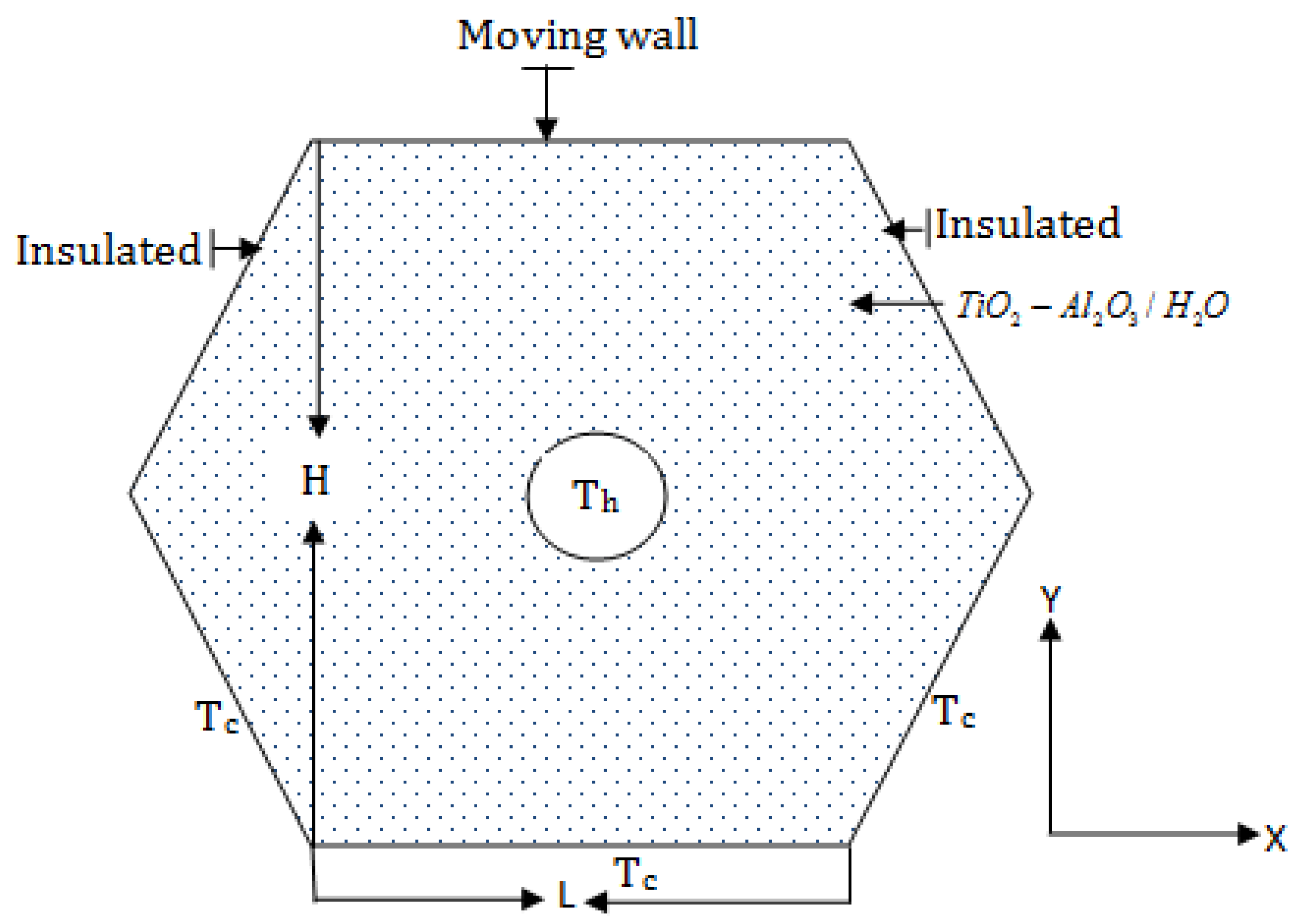
Figure 1 depicts the physical domain with the coordinate system. An incompressible laminar fluid flow in an enclosed space is defined using the Boussinesq approximation. It has been hypothesized that the non-Newtonian (Al2O3-TiO2-H2O)–water nanofluid was contained in the enclosure. In addition, it is anticipated that the base fluid and nanoparticles that are solid will be in thermal equilibrium and moving at an identical rate. Heat exchange performance in the hexagonal enclosure is provided by hot cylinders. The top left and right walls are shown to be adiabatic in Figure 1, while the bottom left, right, and bottom walls are shown to be cooled.
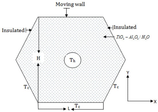
Figure 1.
Schematic diagram of the model considered in this study.
2.1. Non-Newtonian Nanofluid’s Physical Characteristics
Applying the mixture rule as outlined by [35,36] will yield the actual density of the nanofluid:
where denotes the fraction of nanoparticle size, denotes the base fluid’s density, and denotes the solid object’s density. Using the mass averaging method for nanofluids [36], the heat capacity and thermal expansion coefficient of the nanofluid are ascertained:
where the variables and represent the heat capacity and the thermal expansion coefficient of the base fluid, and the variables and represent the heat capacity and thermal expansion coefficient of the solid particle, as well. From the model of Corcione et al. [37,38], the nanofluid’s viscosity is defined as
In this case, the base fluid’s viscosity is , and n is the power law index. The shear rate magnitude might be derived this way by applying the Frobenius norm:
where is the flow shear rate, which can be stated next. The shear rate’s magnitude is :
In the present investigation, the diameter of the base fluid, , is obtained by the following, where the dimension of the nanoparticles is nm:
where kgmol−1 is the molecular weight of the base fluid, and is the Avogadro number. In addition, , the temperature-dependent effective thermal conductivity, is defined in [37,38] and is displayed below:
where , where k is taken into consideration for this study, and , , k (freezing temperature), and and represent the effective thermal conductivity base fluid and nanoparticles, respectively. The thermophysical characteristics of the base fluid and solid ferroparticles were taken from the published literature [39,40,41].
2.2. Characteristics of Hybrid Nanofluids
The following characteristics were obtained from the literature [42,43]:
Concentration on
The term density ()
Dynamic viscosity ()
The term thermal volume heat expansion parameter ()
Parameter for thermal volume heat expansion
Thermal conductivity (k)
The hybrid nanofluid’s heat transfer ratio, , is provided as
where
Electrical conductivity ()
3. Governing Dimensional Equations
The governing equations can be presented as the following:
3.1. Boundary Conditions
As per the illustration in Figure 1, the bottom and lower middle left and right walls are considered cold. Therefore, the temperature, T, is equal to the cold temperature, i.e., . Similarly, the circular surface (heated cylinder) is considered to be heated, and T is equal to , which represents the heated condition. The insulated walls do not contain any heat exchange properties. Based on the aforementioned summary, the boundary conditions of the current problem are as follows.
At bottom and lower middle left and right walls,
On the circular surface,
On the insulated walls,
3.2. Non-Dimensional Formula for Governing Equations
Presenting the subsequent parameters and non-dimensional factors,
Now we change the the governing equations to the dimensionless form by using Equation (26) as follows:
Equation of continuity:
u-Momentum equation:
v-Momentum equation:
Energy equation:
3.3. Physical Quantities
The computation of the heat transfer rate by the Nusselt number can be formulated as both local and average numbers.
The local Nusselt number on the surface of the heated cylinder is depicted as follows:
where the angular coordinate is denoted by . Integrating Equation (31) over the inner cylinder surface yields the calculated :
The surface area of the inner cylinder is represented by s.
4. Thermophysical Properties
The volume fraction of nanoparticles, denoted by , is considered in this study. The symbol represents the volume fraction of alumina (Al2O3) and titanium dioxide (TiO2-H2O). Water functions as the enclosure’s base fluid in the mean time. The thermophysical properties of the base fluid, nanoparticles (Al2O3) and (TiO2-H2O), are displayed in Table 1.

Table 1.
Thermophysical properties of the contents of the hybrid nanofluid [44].
5. Numerical Methods
The present study employs the finite element Galerkin weighted residual technique. The entire fluid domain is divided into non-overlapping triangular elements to determine velocity and temperature using quadratic interpolation functions with four nodes. In contrast, linear interpolation algorithms are used to calculate the pressure gradient. Utilizing these interpolation functions, the dependent variables within each element are approximated in local element coordinates. To solve the governing equations, a set of global nonlinear algebraic equations is generated, and the Newton–Raphson iteration method is applied. Convergence of the weighted residual technique is assessed for all variables, ensuring that the difference between successive iterations, , satisfies the condition , where F is the generic variables. This process for the finite element Galerkin weighted residual technique is described in detail in [45,46].
Grid Independent Test and Code Validation
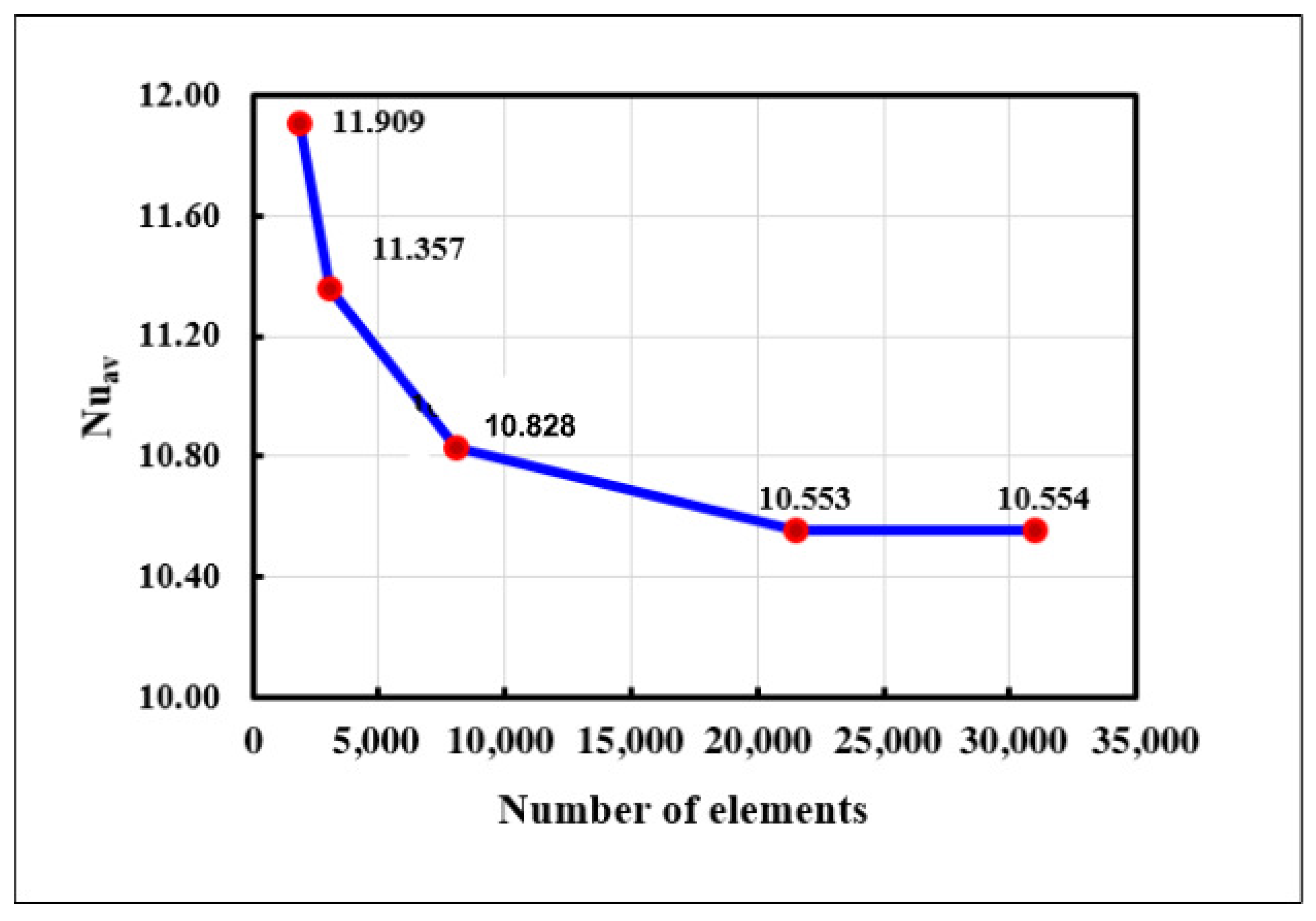
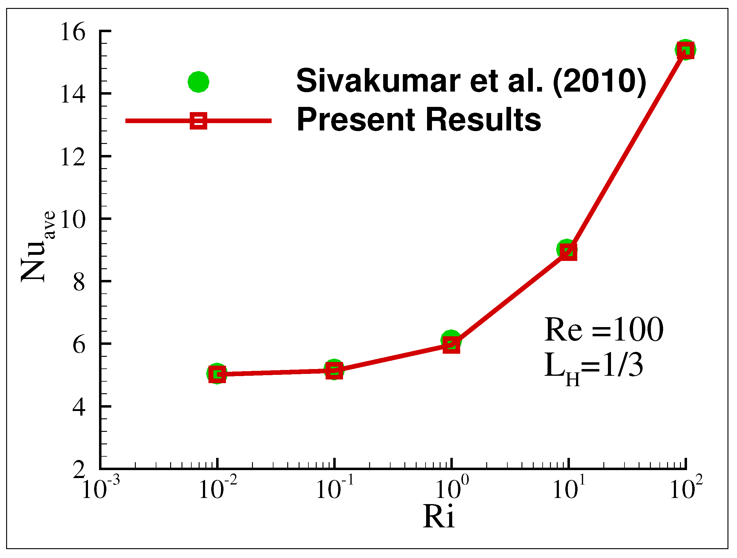
Using the parametric values for the grid independence test, = 300, = 10, = 6.2, and n = 0.6, the ideal number of elements for this finite element method (FEM) is ascertained for this non-Newtonian force convective nanofluid flow model. The domain is partitioned into five sets of triangle elements by the number of elements 1900, 3074, 8078, 21,558, and 31,012, respectively. The magnitudes for the triangle parts 21,558, and 31,012 are nearly equal as Figure 2 illustrates. Therefore, the 21,558 triangle pieces of elements are considered suitable for the study.For the mixed convection, a quantitative comparison of the average Nusselt number () with the results of a study on a lid-driven cavity with a localized heating by Sivakumar et al. [47] is presented in Figure 3 for the conditions , , and . This comparison demonstrates excellent agreement. The code validation for the non-Newtonian power-law fluids and nanofluids were conducted in the previous study by the same authors in [46].
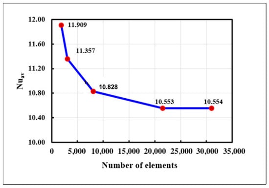
Figure 2.
Grid independence test for the finite element method.

Figure 3.
Quantitative comparison for code validation with the results of Sivakumar et al. [47] in terms of the average Nusselt number () at , , and .
6. Results and Discussion
This study focused on simulating forced convection in a non-Newtonian hybrid nanofluid within a hexagonal enclosure using numerical simulation based on the Galerkin finite element method (GFEM). Due to the consideration of laminar flow under forced convection, numbers started from a lower range at 50, going up to 500 to investigate the sensitivity of the system. The study considered the following parameters: Prandtl number , Reynolds number = 50, 100, 300, 500, power law index n = 0.6, 0.8, 1.0, 1.2, 1.4, nanoparticle volume fractions = 0.0, 0.01, 0.02, 0.03, 0.04, and Hartmann number = 0, 10, 20, 30. The graphical representation of the numerical results are discussed in the following sub-sections:
6.1. Effect of on Streamlines and Isotherms
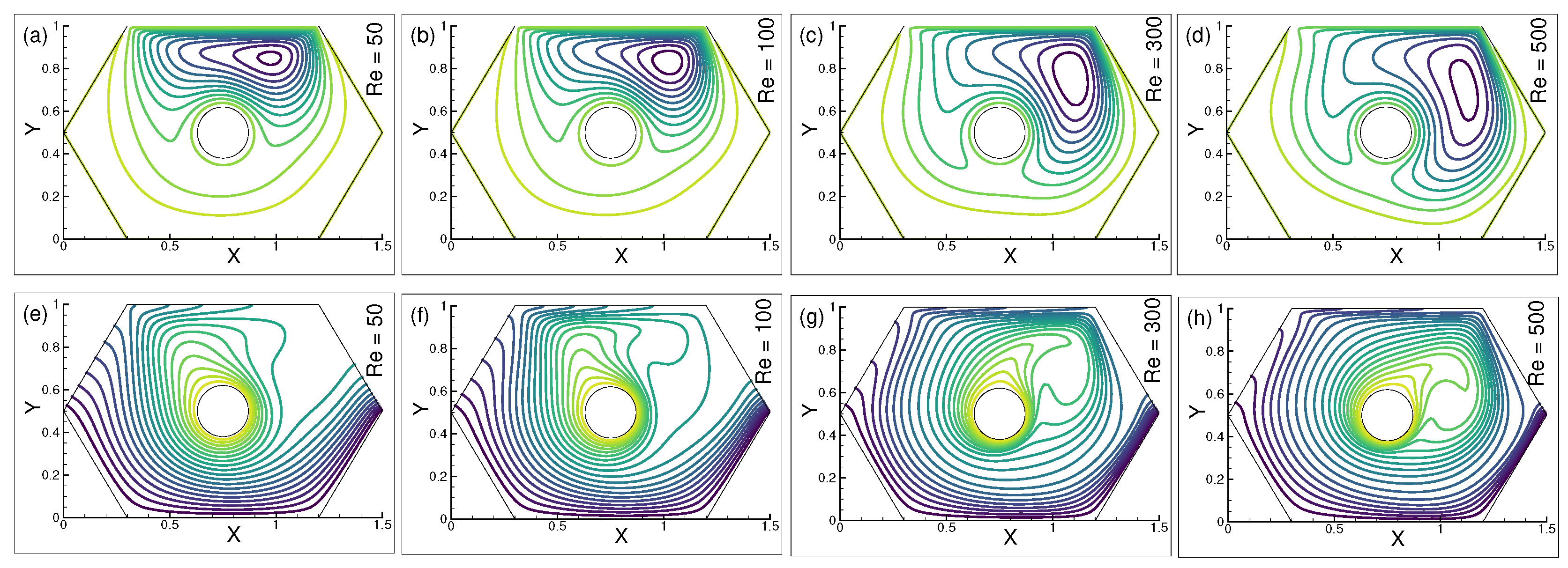
The streamlines and isotherms were obtained for comprehensive qualitative comparisons focusing on the changes in the circulation patterns as , , and varied.Figure 4a–d show how affected streamlines for various values of . The stream gradients are dominant next to the upper walls for = 50, and there is small-scale vorticity in the proximity of the moving wall in Figure 4a. However, beneath the heated circle, three parabolic-shaped recirculations are seen. The dominant streamline and vorticity beneath the upper wall appear as well as they did in the previous Figure 4b. Meanwhile, unique revolving forms appear below as well as on the edge of the right corner. In Figure 4c, the vorticity approaches towards the left corner wall, and the density of the stream gradients declines below the upper wall. A second recirculation can be seen encircling the heated circle, and two larger ones emerge beneath it. In Figure 4d, the gradient density appears sparser as is increased. The size, shape, and location of the vorticity are changed.
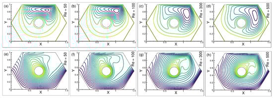
Figure 4.
Changes in (a–d) streamlines and (e–h) isotherms for = 50, 100, 300, and 500, when = , n = and = 10.
Figure 4e–h show the thermal variation for distinct values of . The thermal lines in Figure 4e emerge close to the middle left walls’ base for = 50. The thermal density progressively decreases in the area surrounding the bottom wall. Above the right edge of the heated circle, an additional distinct cavity is formed. This can be attributed to the absence of any temperature gradients in the vicinity of the wall’s top left corner. Temperature gradients in Figure 4f resemble those in the preceding figure, despite the cavities’ slightly different sizes. Figure 4g demonstrates the formation of multiple parabolic-shaped cavities above the right border of the heated circles, as well as a large cavity near the left top corner of the chamber. Inside the chamber, the empty space moves. In Figure 4h, for = 500, the thermal density is noticeably sparser, and a new cavity shape appears close to the enclosure’s left corner wall. There is low movement of fluid in the cavity’s center and an active high-velocity gradient near the walls. The velocity gradient increases at the circular surrounds and decreases near the walls as the cells grew sparser and bigger, indicating that the thermal expansion seems to be potent for all frames.
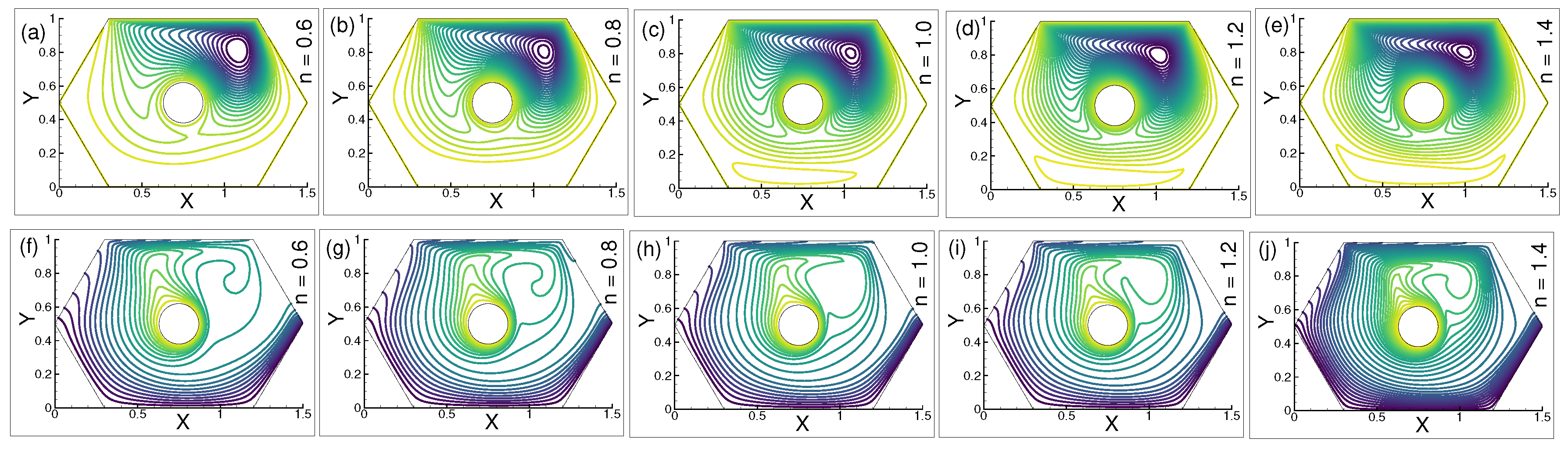
6.2. Effect of Power Law Index n on Streamlines and Isotherms
The effect of the power law index (n) on streamlines is demonstrated in Figure 5a–e. At n = in Figure 5a, the streamlines assemble close to the upper moving wall, developing additional tiny vortices. A substantial vortex can be detected in the right middle corner, while a single, asymmetrical vortex can be seen in the left middle corner and beneath the chamber’s walls. In Figure 5b, the shape and size of the vorticity improve considerably in the middle right corner as the viscosity increases at the point n = , and the number of vortices increases in the middle left corner in a similar manner. Conversely, a large vortex can be seen beneath the upper wall, and the stream gradients seem to be dominant next to it. Figure 5c for the Newtonian case, n = , shows a noticeable change. All recirculations around the left and right borders are also developed, and there is a large vortex below the upper moving wall, around which the stream gradients gather. Taking into consideration the preceding illustrations, the number of recirculations is increased as seen in Figure 5d for viscosity n = . Additionally, the streamlines appear below the heated circle. The large recirculation approaching near the right middle corner and stream gradients seem to be more developed below the upper wall which is visible in Figure 5e for n = . The vortices that form beneath the upper wall nearly diminish as a result of the increasing viscosity. The density of the streamline also decreases in the heated circle’s left and right borders.

Figure 5.
Evolutions of (a–e) streamlines and (f–j) isotherms for n = , , , , and , when = , = and = 300.
The isothermal lines in Figure 5f are mostly visible beneath the heated circle, and their density gradually decreases as one approaches the bottom wall. The upper and left upper walls of the heated circle are formed by the thermal cavities. In addition to the thermal lines being visible in Figure 5g similar to the earlier figure, the distribution of the isotherms starts to increase. In Figure 5h, the thermal lines start to vanish in the upper left wall, and further cavities can be observed close to the upper right corner. Figure 5i,j show the newly formed thermal cavities beneath the upper moving wall as the viscosity increases at . However, the isotherms demonstrate no discernible change from the previous figures.
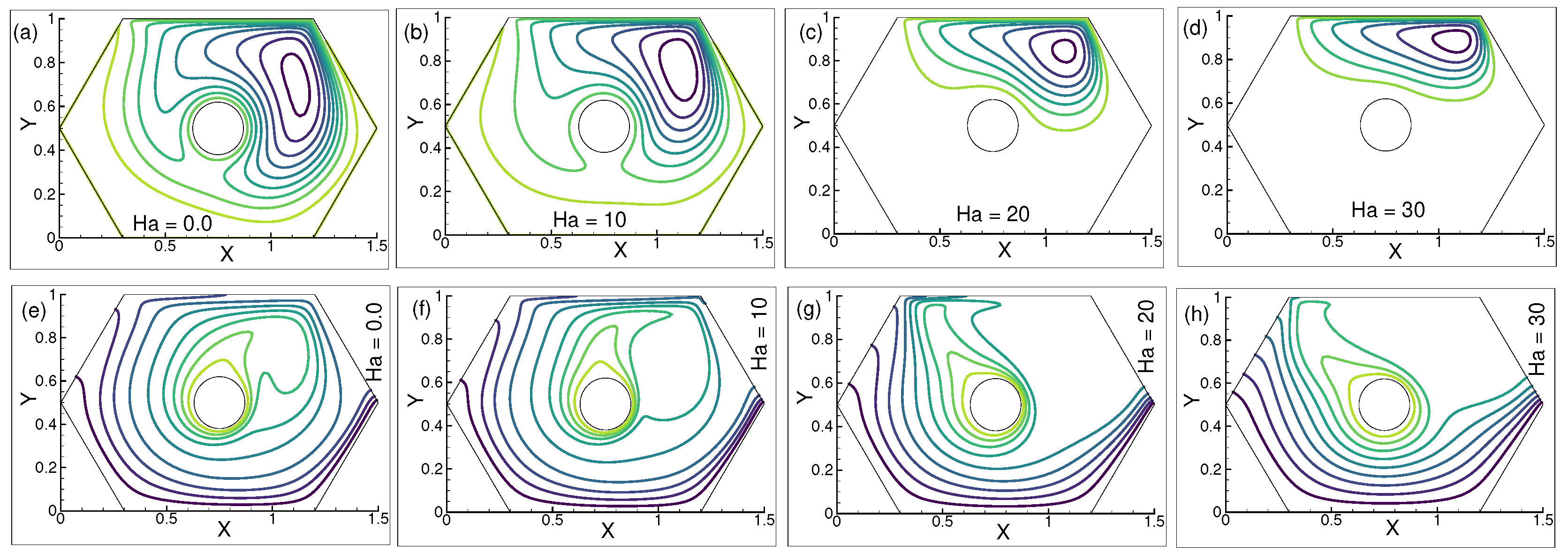
6.3. Impact of on Streamlines and Isotherms
Figure 6a–d display the streamlines for a selection of values. The stream gradients are the most visible next to the moving wall in Figure 6a, and for = 0, additional vortices form next to the top left corner of the enclosure. Compared to the region above the circles, the streamlines below the circles appear more sparse. In Figure 6b, the streamlines below the circles drastically diminish but stay at the same level beneath the moving wall and in the upper left corner. Figure 6c,d show that for = 20 to 30, there is only a partial recirculation below the heat circle, which leaves a space between the stream curve and below the circle void. Compared to the preceding figure, the vorticity size beneath the upper wall appears to be smaller.
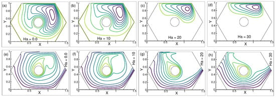
Figure 6.
Influence on (a–d) streamlines and (e–h) isotherms for = , , , and at fixed = 300, n = and = .
Moreover, Figure 6e–h show the thermal distribution for changing while keeping the values for n = , = 300, and = constant. The formation of variously shaped thermal cavities above the left corner and the gathering of isothermal lines at the bottom wall are depicted in Figure 6e. In Figure 6f, a big cavity forms. In the enclosure, below the upper left wall and next to the middle left wall, there is a void. A larger parabolic-shaped cavity is formed above the right edge of the heated circle. Figure 6g,h illustrate that a large vacuum forms beneath the upper left wall for = 20 to 30, and a changing size of the thermal cavity above the circle’s right corner. As they approach the bottom walls of each figure, the heated circle, the isotherms disperse, and the temperature gradients become less apparent. There are sizeable regions where the thermal lines can be seen beneath the enclosure’s left and right walls.
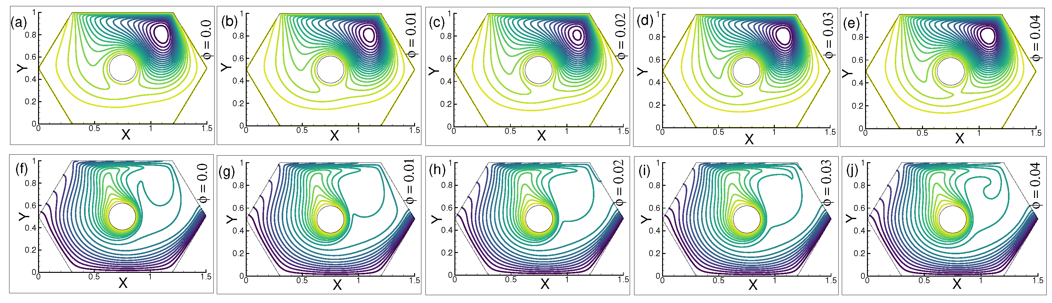
6.4. Influence of on Streamlines and Isotherm
The effects of = , , and on the streamline patterns for constant n = , = 10, and = 300 are shown in Figure 7a–c. Numerous vortices form close to the top left corner of the chamber, and there are a good number of recirculations from below the heated cylinder. The dominant gradients of the stream can be seen next to the moving wall. The stream gradients in Figure 7d,e appear sparser as the volume fraction increases. A solitary vortex can be seen beneath the heated cylinder in Figure 7e. In addition, Figure 7f–j show the distribution of isotherms for various values of . The thermal lines for = 0 are shown in Figure 7f. A number of cavities emerge above the right edge heated cylinder as thermal gradients congregated close to the wall at the bottom. Adjacent to the enclosure’s upper left corner, a sizeable cavity develops. For = , the distribution of isotherms in Figure 7g marginally changes above the heated cylinder, and a significant vacuum develops close to the upper left wall.
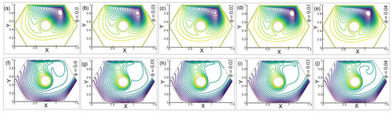
Figure 7.
Changes in the patterns of (a–e) streamlines, and (f–j) isotherms for = , , , and , when = , = 300, = 10, and n = .
Moreover, Figure 7h,i show that the streamlines dominate the bottom wall as the value of augments. An isothermal line of nearly the identical shape is visible near the upper corner of the enclosure. In Figure 7j, a more developed isothermal density is observed close to the base of the moving wall, leaving a void in the proximity of the middle left wall for = .
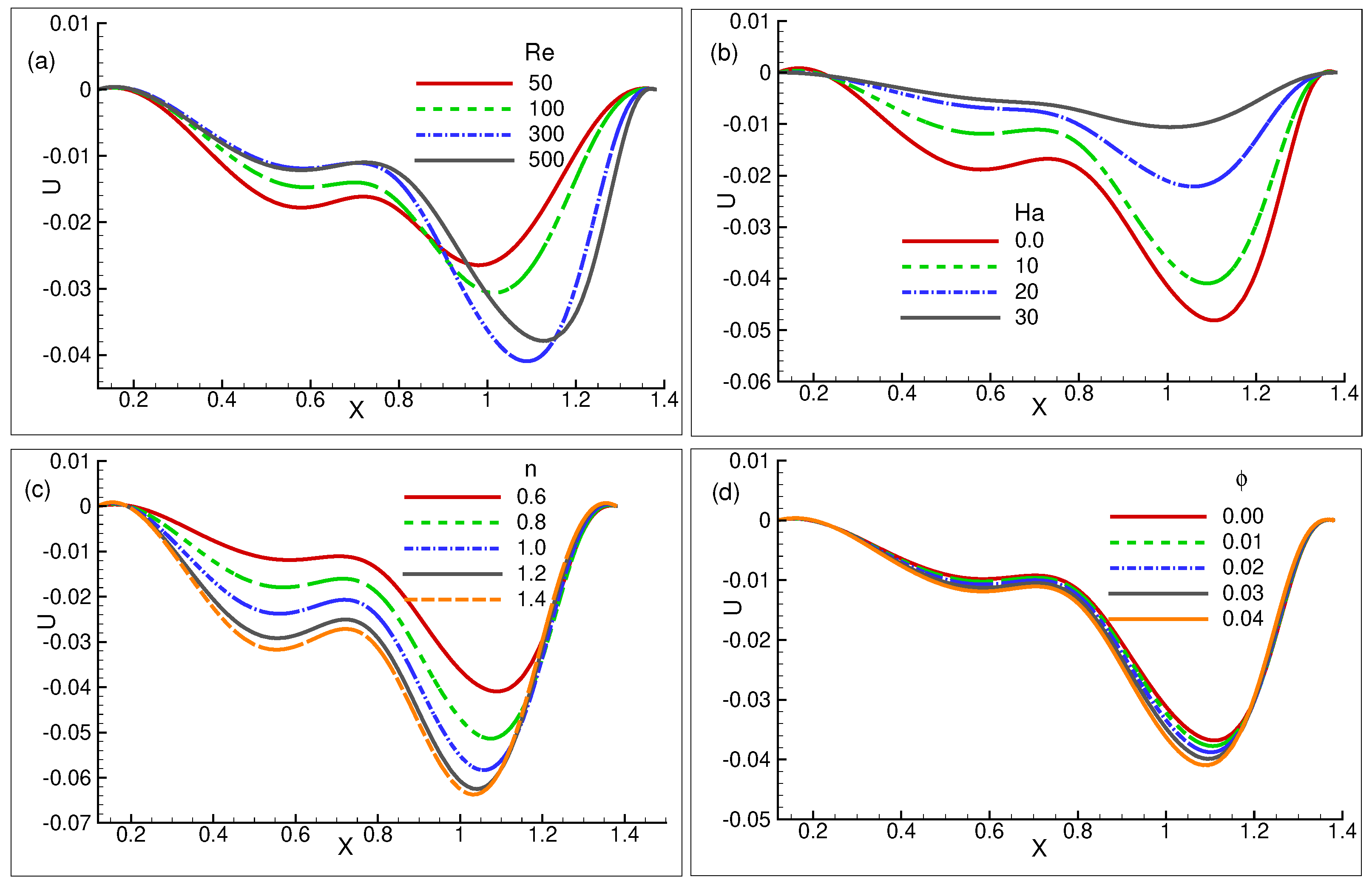
6.5. Distribution of Velocity for , , , and n
Figure 8a demonstrates the horizontal velocity components for the various numbers at the point y = . For a higher value of , the velocity profile propagates with higher magnitudes as follows from the point 0 where it originates. The velocity profiles all exhibit negative magnitudes as they begin to decline from the origin 0. Eventually, all of the curves come together at x = . Due to the dominance of the buoyancy force, velocity profiles follow the longest path in the domain as the number is increased. For = 500, the largest magnitude is apparent at x = . Figure 8b illustrates the variation in the velocity profiles. The velocity profiles all decrease after they overcome the origin 0. The largest positive magnitude for = is visible at x = , and as increases from to 30, it gradually decreases in magnitude. For = 30, a smooth, straight curve is evident, while for = 0, a further distorted curve is noticed. The variations in the power law-index n = , , , , and have the impact on the velocity distribution along the line x at y = as shown in Figure 8c. The velocity profiles all decrease after they cross the origin 0. The largest positive magnitude for = is visible at x = , and as increases from to 30, it gradually decreases in magnitude. Due to the viscosity n = , the velocity moves quickly along the short path. The magnitudes of the velocity profiles exhibit a progressive decline in values as n increases, reaching a maximum negative value that is minimal at x = for n = , which is perceptible.
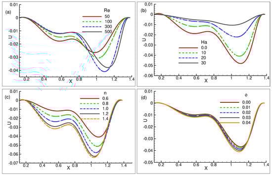
Figure 8.
Velocity profiles (a) for = 50, 100, 300, and 500 (b) for = , 10, 20, and 30 (c) for n = , , , , and for constant values = 10, = and = 300, (d) for = , , , , and .
Moreover, Figure 8d illustrates the variation in the velocity profiles. The velocity profiles all decrease after they depart from the origin 0. The largest positive magnitude for = is visible at x = , and as increases from to 30, it gradually decreases in magnitude. Figure 8d displays the velocity profiles for setting the values of = 300, n = , as well as = 10 to emphasize the effect in the velocity profiles.The base fluid = shows the highest scale in the velocity profile. The peak amplitudes of profiles gradually plummet from positive to negative as the volume fraction starts to increase. The velocity path displays a sign shift from negative to positive. The entire velocity profile path exhibits visible compactness, and the change in velocity path is insignificant.
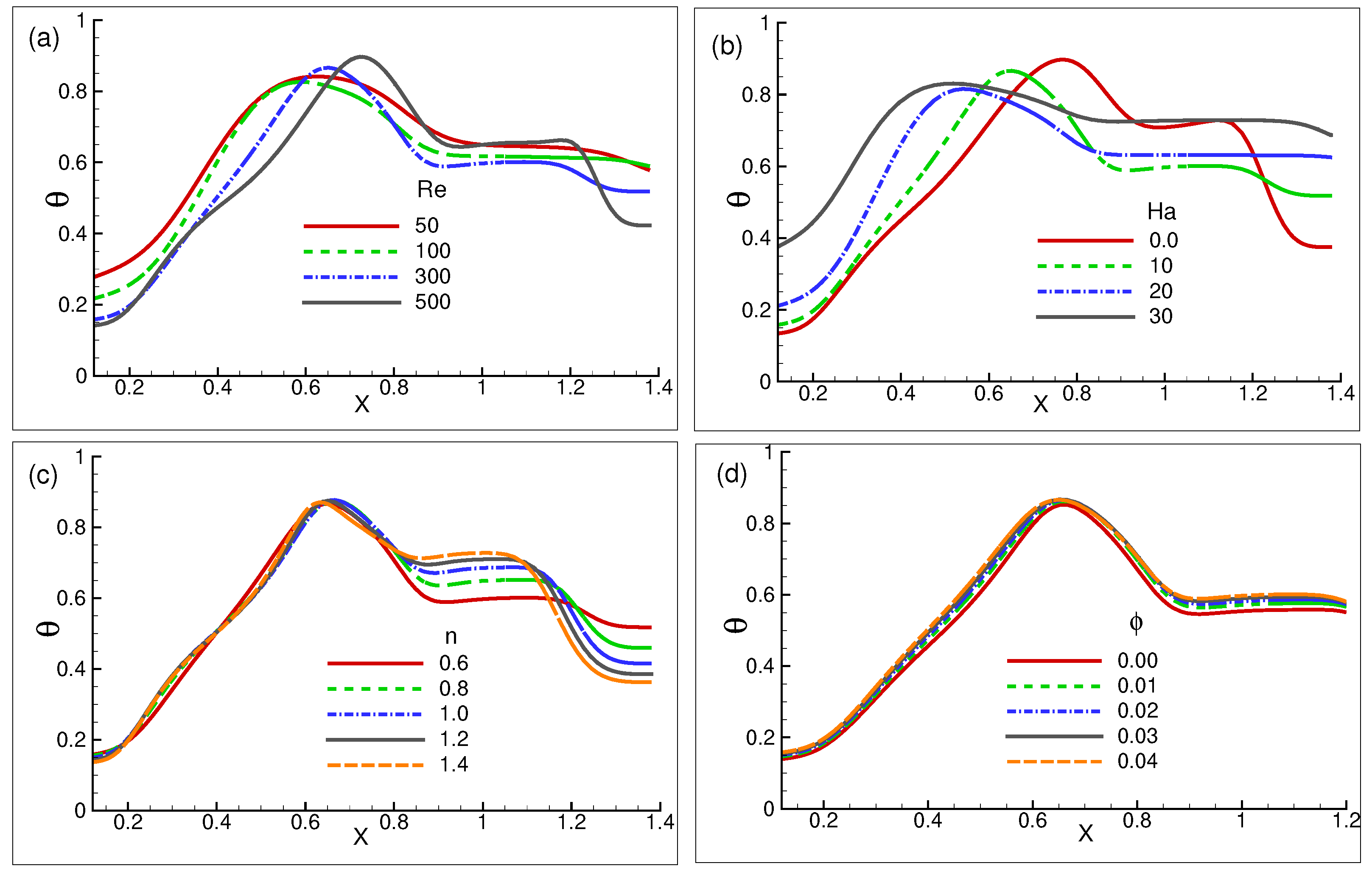
6.6. Evolution of Temperature for ,, and n
The thermal distribution for the variation in at y = is shown in Figure 9a. As goes up, the peak of the amplitudes gradually declines, with a noticeable exception at = 500. The distribution clearly illustrates that for = 300 and 500, the thermal path is shown to be irregular after their magnitudes. Furthermore, the figure makes it evident that as increases, the thermal performance becomes more well distributed. In addition, for fixed = 300, n = , and = , the influence of temperature distribution for the Hartman number is illustrated in Figure 9b. At x = , the temperature profile of = reaches its maximum amplitude even though it starts from a lower level. The temperature movement begins slightly higher than the preceding curve and appears to be lesser in magnitude as is increased to 10. The temperature profiles for = 20 to 30 exhibit ascending magnitude levels from beginning to end. Following their peak amplitude, all of the temperature curves exhibit a downward trend. Meanwhile, Figure 9c shows the thermal distribution with respect to the various power law index n values. Following the point x = 7, the temperature movement path n = appears to be a straight line. For all values of n, the temperature magnitude reaches its maximum at x = . After that, it gradually declines as the power law index increases. For every power law index n, the thermal variation is visible after the points x= . At x = , the convection rate is observed to be the opposite result for all power law indexes n.
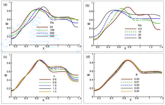
Figure 9.
Temperature profiles of (a) for = 50, 100, 300, and 500 for set = , = 10 and n = (b) for = , 10, 20, and 30, while for set n = , = and = 300, (c) for n = , , , , and while for set = 10, = 300, and = (d) for = , , , , and , while for set = 10, = 300,and n = at the point y = .
Figure 9d displays the impact of variation in temperature on various values of in order to look for patterns in the temperature profile. At x = , the temperature scale appears lower for base fluid = . At x = , the maximum magnitude is created for = , and the temperature magnitude increases progressively as the value of increases from to . The temperature curve sharply decreases after x = , reaching its lowest temperature magnitudes at x = , plays a significant role in the force convection flow trend due to the proportionate relationship between convection characteristics and the fluid volume fraction.
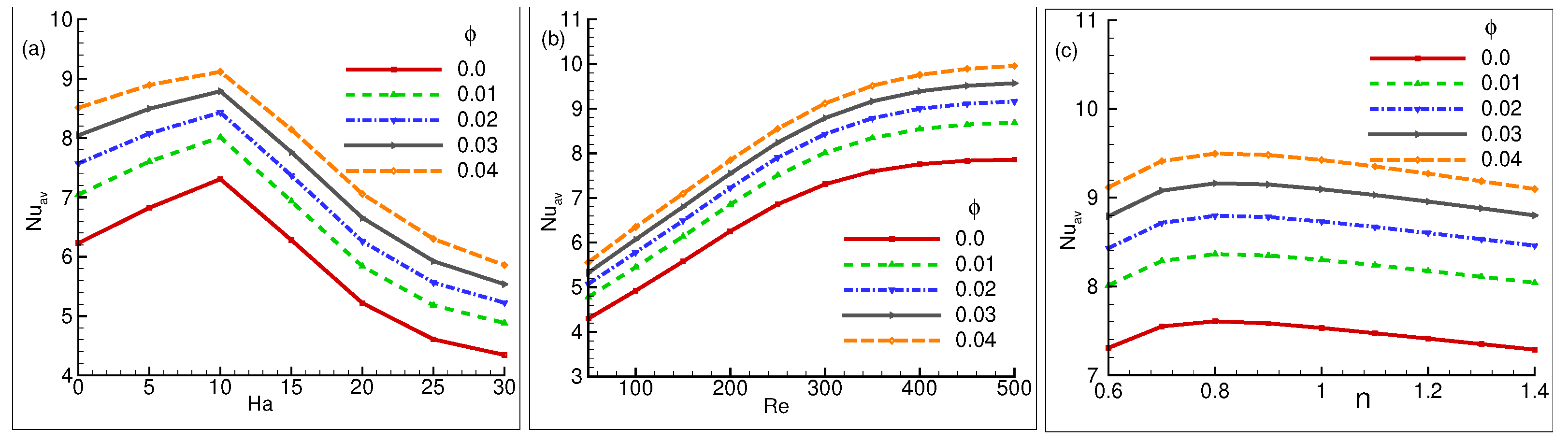
6.7. Changes in Average Nusselt Numbers
Figure 10a–c illustrate how the average Nusselt for cylinder behaves with relation to heat transport when is changed. Figure 10a illustrates how the heat transfer rate of seems to be getting bigger for = 0 to 5 and then decreasing for = . For the values ranging from = 0 to 5, the thermal rate enhances with increasing the value of , but it then starts to decline with increasing . The declines from = 5 to 30 for each case as augments. For = , the begins to rise at y = for the value of = 0 to 5. However, it then begins to decline again, commencing at points and progressively declining with the augmentation of both and . Furthermore, Figure 10b illustrates the average Nusselt number given the variance in as well as . For = , the conductivity rate increases. As both and improve, the rate of heat transfer increases. From the range = 400 to 500, the rate of improvement in thermal conductivity is found to be declining. Finally, the average Nusselt number for the variation of and the power law index n is presented in Figure 10c. At = 0, the heat transfer rate increases after rising from n = to , and it gradually plummets to n = . For n = to , the heat transfer rate seems to improve while the amount of increases, but it then begins to progressively drop once more. As increases, the thermal lines exhibit an improved peak values as well, as seen in the figure.
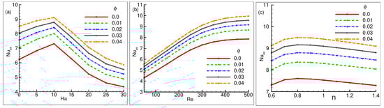
Figure 10.
Variations of for (a) = , 10, 20, and 30 (b) = 50, 100, 300, and 500 (c) n = , , , , and .
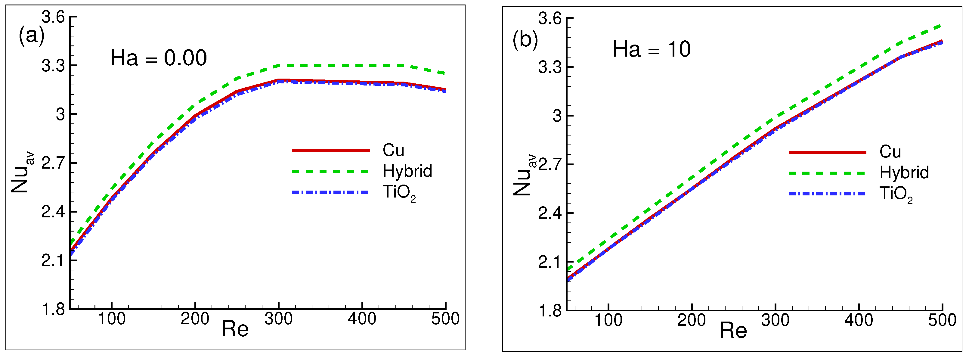
The for , , and both of the combined nanofluids are shown in Figure 11a,b for = , for the fixed values of = 300 and n = . The hybrid nanofluid is positioned higher than the individual two as can be seen in both figures. The integration of a single-phase nanofluid (either or ) does not seem to make any difference, as their corresponding curves overlap each other. This is an evidential outcome that hybrid nanofluids improve the thermal efficiency by increasing the average rate of heat transfer.
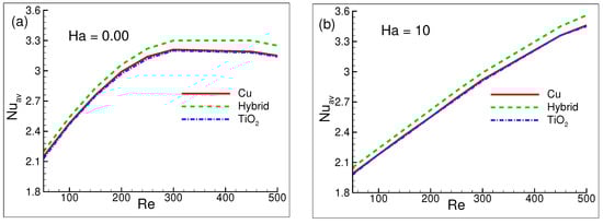
Figure 11.
Average Nusselt number variations for (a) = and (b) = while = = , and = 300, n = .
6.8. Statistical Analysis and Parametric Sensitivity Tests
6.8.1. Correlation Development
The response surface methodology (RSM) is a well-known statistical analytic technique to develop correlations among input variables with a view to developing a prediction equation [48]. The second-order model often produces a good estimate of the response, even in cases where there are other RSM models. As reported in the literature, the quadratic RSM model is [48]
In this case, , , , , , , , , , and are the coefficients of the corresponding terms, and y is the output function. Finding the response function that matches the closest to the interaction between independent parts is the primary goal. In this case, a second-order RSM model based on central composite design (CCD) is used [49]. This RSM model is based on CCD, and it has 20 runs total for 3 independent factors: 6 center, 8 cube, and 6 axial points per factor. The coded level for the CCD-based RSM is shown in Table 2. In addition, Table 3 expresses the real values, response function values, and 20 runs of coded values. In this study, the RSM explains how the response function () is affected by the included parameters (, , and ).
Table 2.
Coded levels and design variables for CCD.
Table 3.
Levels of input factors and response function.
Furthermore, Table 4 presents the results of the RSM statistical exploration conducted on this model. The degrees of freedom (DOF) denote the maximum number of independent terms. Additionally, the p-value indicate the likelihood that the null hypothesis would hold true for a specific statistical model. The model is considered significant when the p-value is smaller, usually <, as this indicates that the null hypothesis is rejected. Although the model possesses a less adjusted value (), the statistical analysis and testing methods show that the () for is indeed superior, suggesting that this model is appropriate for generating the response function . Lack-of-fit is another important statistic that needs to be incredibly modest in order for a model to be considered appropriate. After completing this investigation using RSM, the coefficients of Equation (33) are obtained. As a result, the initial correlation of Equation (33) among the response function y () and the independent factors , and are obtained in appropriate form, and this relation is expressed as a coded unit which is in Equation (34):
Table 4.
Analysis of variance for .
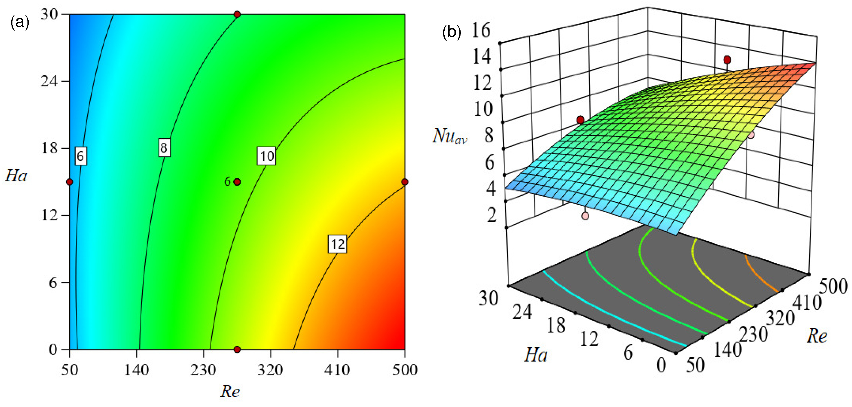
6.8.2. Response Surface Analysis
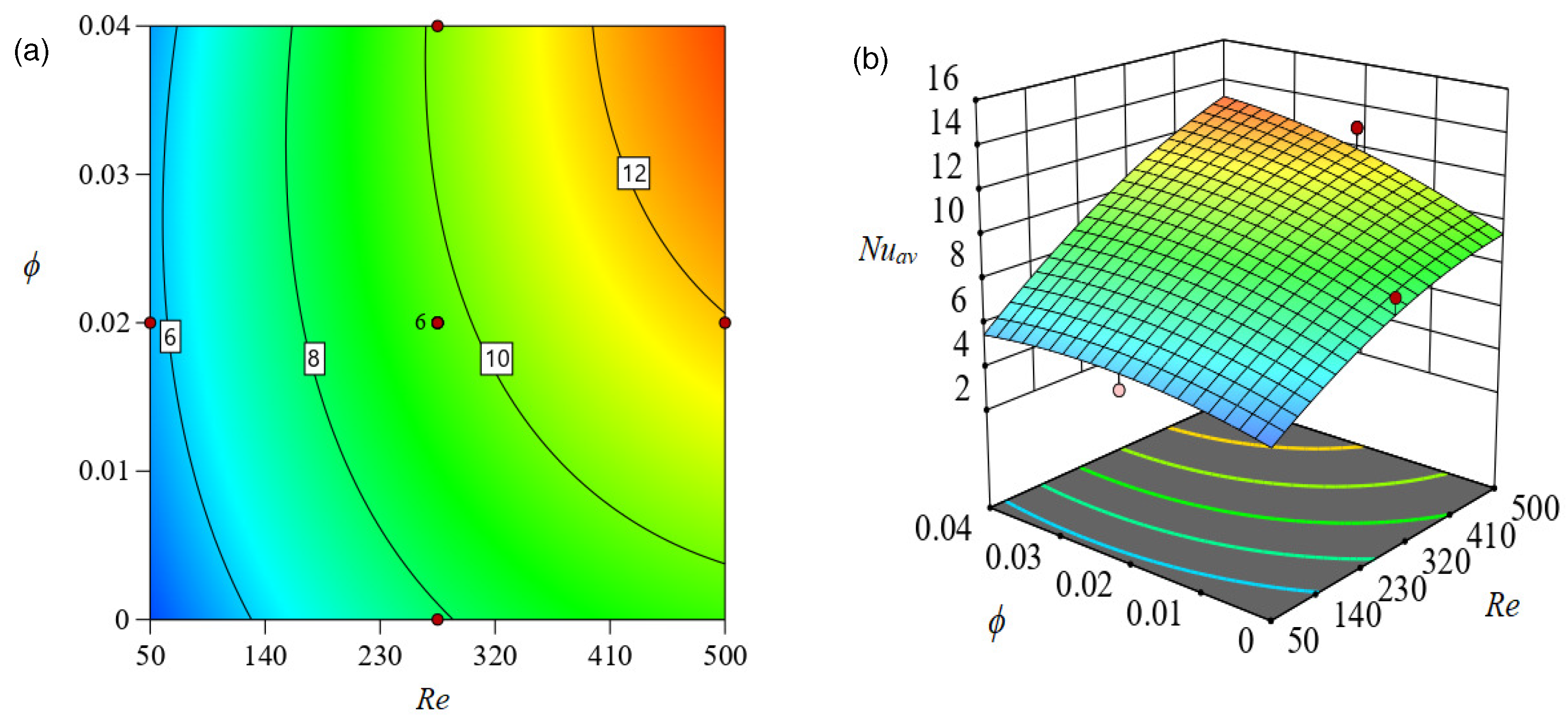
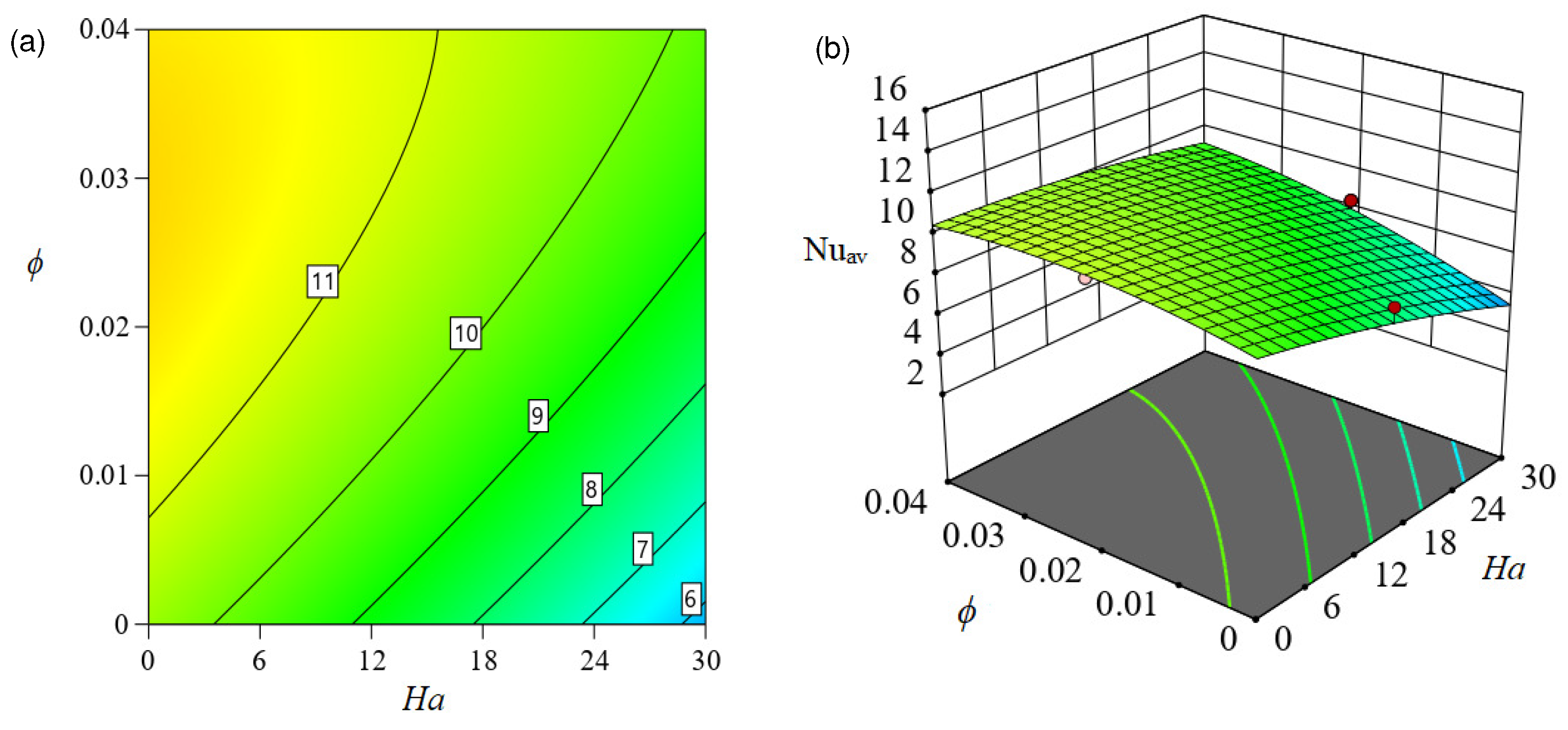
Figure 12, Figure 13 and Figure 14 present and contour plots, respectively, about the response surface developed using RSM (to predict ) in order to evaluate the influence of independent factors on the response function. The response of to and is visualized in Figure 12. Evidently, the response function is augmented for but decreased for as this contour map makes evident. When is increased from 50 (coded value −1) to 275 (coded value 0), the rate of heat transmission is increased by around . Furthermore, the increases by approximately when the magnitude of increases from 275 (coded value 0) to 500 (coded value 1). The contour in Figure 12a shows that the fluctuation rate of is at the largest magnitude of and the lowest value of (coded value −1). Likewise, Figure 14 illustrates the concurrent impact of and on . Here, the changing rate of is developed by increasing the size of while decreasing the magnetic field strength (). Nevertheless, the rate of changing in is lower than it was in the prior two cases.
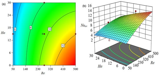
Figure 12.
Effect of and on in (a) (b) .
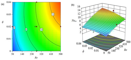
Figure 13.
Effect of Re and on in (a) (b) .
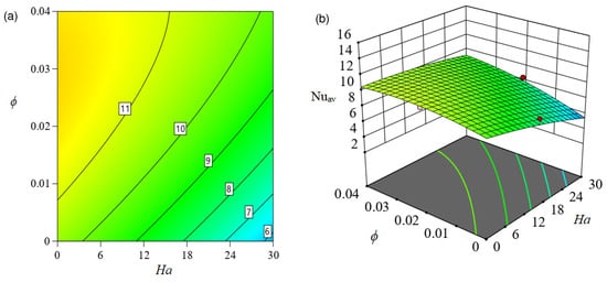
Figure 14.
Effect of Ha and on in (a) (b) .
7. Conclusions
The present research employed a numerical model to look into forced convection with a heated cylinder embedded in the hexagonal chamber in order to examine the non-Newtonian power-law hybrid nanofluids. It was shown that the non-dimensional components, such as , n, , and , influenced the outcomes. The results could be comprehended both numerically and visually when the outline presented the numerical data. The investigation was carried out using the finite element analysis method. The analysis, which was performed for various values of the aforementioned parameters, produced the following key findings:
- (I)
- The heat transfer of non-Newtonian hybrid nanofluid fluids, thermal velocity, power law index (n), nanoparticle volume fraction (), Hartman number (), and numbers all possessed considerable effects on the fluid characteristics.The maximum exhibited more stable distribution of velocity profiles. However, as was imposed, the fluid demonstrated quasi-static behavior, regardless of the numbers. The power law fluid showed more stable response in terms of fluid mobility, whereas fluid corresponding to would require elevated numbers to stabilize the system. The impact of on velocity distribution had a marginal impact compared to other dimensionless parameters.
- (II)
- As , n, and increased, the average Nusselt number increased but the opposite outcome was observed at . The maximum value of average was obtained at , , and ( nanoparticles). The outcome was more thermally efficient for .
- (III)
- The temperature profiles, however, yielded the maximum value at at a non-zero number. The temperature profiles were more impacted by and rather than n or .
- (IV)
- The hybrid nanofluid improved the rate of heat transfer by approximately comparing to a single-phase nanofluid system (either or ).
Further investigations could be conducted in the future by extensively focusing on the uniformity index of the heated walls of the enclosure. At higher numbers, the effect of heat transfer and temperature gradient will be accelerated, leading to an improvement in the uniformity index of the heating surface. In the future, this will also provide improved insights on the cooling mechanism of the enclosure containing hybrid nanofluids.
Author Contributions
M.N.-A.-A.S.: Conceptualization, data curation, formal analysis, methodology, writing—original draft; S.I.: Conceptualization, data curation, formal analysis, methodology, writing—original draft; M.U.A.: formal analysis, methodology, writing—original draft; M.F.H.: formal analysis, methodology, writing—original draft; M.M.M.: Conceptualization, data curation, formal analysis, methodology, funding acquisition, project administration, supervision. All authors have read and agreed to the published version of the manuscript.
Funding
(i) North South University, Grant No.: CTRG-24-SEPS-05, (ii) Ministry of Science and Technology, Bangladesh Government (Appl. No.: 1717932033 for 2024–2025).
Data Availability Statement
Data can be shared upon request. The manuscript is not associated with any third party data.
Conflicts of Interest
The authors declare no conflicts of interest.
References
- Arif, M.; Suneetha, S.; Basha, T.; Reddy, P.B.A.; Kumam, P. Stability analysis of diamond-silver-ethylene glycol hybrid based radiative micropolar nanofluid: A solar thermal application. Case Stud. Therm. Eng. 2022, 39, 102407. [Google Scholar] [CrossRef]
- Anee, M.J.; Siddiqa, S.; Hasan, M.F.; Molla, M.M. Lattice Boltzmann simulation of natural convection of ethylene glycol-alumina nanofluid in a C-shaped enclosure with MFD viscosity through a parallel computing platform and quantitative parametric assessment. Phys. Scr. 2023, 98, 095203. [Google Scholar] [CrossRef]
- Choi, S.U.; Eastman, J.A. Enhancing Thermal Conductivity of Fluids with Nanoparticles; Technical Report; Argonne National Lab. (ANL): Argonne, IL, USA, 1995. [Google Scholar]
- Khan, U.; Zaib, A.; Bakar, S.A.; Ishak, A. Stagnation-point flow of a hybrid nanoliquid over a non-isothermal stretching/shrinking sheet with characteristics of inertial and microstructure. Case Studies Therm. Eng. 2021, 26, 101150. [Google Scholar] [CrossRef]
- Khetib, Y.; Abo-Dief, H.M.; Alanazi, A.K.; Said, Z.; Memon, S.; Bhattacharyya, S.; Sharifpur, M. The Influence of Forced Convective Heat Transfer on Hybrid Nanofluid Flow in a Heat Exchanger with Elliptical Corrugated Tubes: Numerical Analyses and Optimization. Appl. Sci. 2022, 12, 2780. [Google Scholar] [CrossRef]
- Nikushchenko, D.; Pavlovsky, V.; Nikushchenko, E. Fluid Flow Development in a Pipe as a Demonstration of a Sequential Change in Its Rheological Properties. Appl. Sci. 2022, 12, 3058. [Google Scholar] [CrossRef]
- Muneeshwaran, M.; Srinivasan, G.; Muthukumar, P.; Wang, C.C. Role of hybrid-nanofluid in heat transfer enhancement–A review. Int. Comm. Heat Mass Transf. 2021, 125, 105341. [Google Scholar] [CrossRef]
- Xiong, Q.; Altnji, S.; Tayebi, T.; Izadi, M.; Hajjar, A.; Sundén, B.; Li, L.K. A comprehensive review on the application of hybrid nanofluids in solar energy collectors. Sustain. Energy Technol. Assess. 2021, 47, 101341. [Google Scholar] [CrossRef]
- Hussain, S.M.; Jamshed, W. A comparative entropy based analysis of tangent hyperbolic hybrid nanofluid flow: Implementing finite difference method. Int. Comm. Heat Mass Transf. 2021, 129, 105671. [Google Scholar] [CrossRef]
- Anee, M.J.; Hasan, M.F.; Siddiqa, S.; Molla, M.M. MHD Natural Convection and Sensitivity Analysis of Ethylene Glycol Cu-Al2O3 Hybrid Nanofluids in a Chamber with Multiple Heaters: A Numerical Study of Lattice Boltzmann Method. Int. J. Energy Res. 2024, 2024, 5521610. [Google Scholar] [CrossRef]
- Ahmad, F.; Abdal, S.; Ayed, H.; Hussain, S.; Salim, S.; Almatroud, A.O. The improved thermal efficiency of Maxwell hybrid nanofluid comprising of graphene oxide plus silver/kerosene oil over stretching sheet. Case Stud. Therm. Eng. 2021, 27, 101257. [Google Scholar] [CrossRef]
- Jamshed, W.; Alanazi, A.K.; Isa, S.S.P.M.; Banerjee, R.; Eid, M.R.; Nisar, K.S.; Alshahrei, H.; Goodarzi, M. Thermal efficiency enhancement of solar aircraft by utilizing unsteady hybrid nanofluid: A single-phase optimized entropy analysis. Sustain. Energy Technol. Assess. 2022, 52, 101898. [Google Scholar] [CrossRef]
- Abbasi, A.; Al-Khaled, K.; Khan, M.I.; Khan, S.U.; El-Refaey, A.M.; Farooq, W.; Jameel, M.; Qayyum, S. Optimized analysis and enhanced thermal efficiency of modified hybrid nanofluid (Al2O3, CuO, Cu) with nonlinear thermal radiation and shape features. Case Studies Therm. Eng. 2021, 28, 101425. [Google Scholar] [CrossRef]
- Jana, S.; Salehi-Khojin, A.; Zhong, W.H. Enhancement of fluid thermal conductivity by the addition of single and hybrid nano-additives. Thermochim. Acta 2007, 462, 45–55. [Google Scholar] [CrossRef]
- Alharbi, A.A.; Alzahrani, A.R.R. A COMSOL-Based Numerical Simulation of Heat Transfer in a Hybrid Nanofluid Flow at the Stagnant Point across a Stretching/Shrinking Sheet: Implementation for Understanding and Improving Solar Systems. Mathematics 2024, 12, 2493. [Google Scholar] [CrossRef]
- Nihaal, K.M.; Mahabaleshwar, U.S.; Swaminathan, N.; Laroze, D.; Shevchuk, I.V. A Numerical Investigation of Activation Energy Impact on MHD Water-Based Fe3O4 and CoFe2O4 Flow between the Rotating Cone and Expanding Disc. Mathematics 2024, 12, 2530. [Google Scholar] [CrossRef]
- Alhowaity, A.; Bilal, M.; Hamam, H.; Alqarni, M.; Mukdasai, K.; Ali, A. Non-Fourier energy transmission in power-law hybrid nanofluid flow over a moving sheet. Sci. Rep. 2022, 12, 10406. [Google Scholar] [CrossRef]
- Bilal, S.; Khan, N.Z.; Shah, I.A.; Awrejcewicz, J.; Akgül, A.; Riaz, M.B. Heat and flow control in cavity with cold circular cylinder placed in non-newtonian fluid by performing finite element simulations. Coatings 2021, 12, 16. [Google Scholar] [CrossRef]
- Nadeem, S.; Hamed, Y.; Riaz, M.B.; Ullah, I.; Alzabut, J. Finite element method for natural convection flow of Casson hybrid (Al2O3–Cu/water) nanofluid inside H-shaped enclosure. AIP Adv. 2024, 14, 085130. [Google Scholar] [CrossRef]
- Zahid, F.; Riaz, M.B. Computational analysis of EMHD nanofluid flow over a thermally conductive surface: Enhancing heat transfer for industrial applications. Int. J. Thermofluids 2024, 25, 100987. [Google Scholar] [CrossRef]
- Niihara, K. New design concept of structural ceramics ceramic nanocomposites. J. Ceram. Soc. Jpn. 1991, 99, 974–982. [Google Scholar] [CrossRef]
- Suresh, S.; Venkitaraj, K.; Selvakumar, P.; Chandrasekar, M. Synthesis of Al2O3–Cu/water hybrid nanofluids using two step method and its thermo physical properties. Colloids Surf. A Physicochem. Eng. Asp. 2011, 388, 41–48. [Google Scholar] [CrossRef]
- Nadeem, S.; Abbas, N.; Khan, A. Characteristics of three dimensional stagnation point flow of Hybrid nanofluid past a circular cylinder. Res. Phys. 2018, 8, 829–835. [Google Scholar] [CrossRef]
- Hayat, T.; Nadeem, S.; Khan, A. Rotating flow of Ag-CuO/H2O hybrid nanofluid with radiation and partial slip boundary effects. Eur. Phys. J. E 2018, 41, 75. [Google Scholar] [CrossRef] [PubMed]
- Nadeem, S.; Abbas, N. On both MHD and slip effect in micropolar hybrid nanofluid past a circular cylinder under stagnation point region. Can. J. Phys. 2019, 97, 392–399. [Google Scholar] [CrossRef]
- Sheikholeslami, M.; Mehryan, S.; Shafee, A.; Sheremet, M.A. Variable magnetic forces impact on magnetizable hybrid nanofluid heat transfer through a circular cavity. J. Mol. Liq. 2019, 277, 388–396. [Google Scholar] [CrossRef]
- Hassan, M.; Ellahi, R.; Bhatti, M.M.; Zeeshan, A. A comparative study on magnetic and non-magnetic particles in nanofluid propagating over a wedge. Can. J. Phys. 2019, 97, 277–285. [Google Scholar] [CrossRef]
- Subhashini, S.; Sumathi, R. Dual solutions of a mixed convection flow of nanofluids over a moving vertical plate. Int. J. Heat Mass Transf. 2014, 71, 117–124. [Google Scholar] [CrossRef]
- Hasan, M.F.; Himika, T.A.; Molla, M.M. Large-eddy simulation of airflow and heat transfer in a general ward of hospital. In AIP Conference Proceedings; AIP Publishing: Melville, NY, USA, 2016; Volume 1754. [Google Scholar]
- Hassan, S.; Himika, T.A.; Molla, M.M.; Hasan, F. Lattice Boltzmann simulation of fluid flow and heat transfer through partially filled porous media. Comput. Eng. Phys. Model. 2019, 2, 38–57. [Google Scholar]
- Khan, Y.; Majeed, A.H.; Shahzad, H.; Awan, F.J.; Iqbal, K.; Ajmal, M.; Faraz, N. Numerical computations of non-Newtonian fluid flow in hexagonal cavity with a square obstacle: A hybrid mesh–based study. Front. Phys. 2022, 10, 891163. [Google Scholar] [CrossRef]
- Battira, M.M.; Brahmi, C.; Bessaih, R.; Chadi, K. Forced Convection of Cu-Water Nanofluid in Vented Square Enclosure with an Interior Rotating Hexagonal Cylinder. Int. J. Heat Technol. 2023, 41, 339. [Google Scholar] [CrossRef]
- Molla, M.M.; Hasan, M.F.; Islam, M.M. Elucidating thermal phenomena of non-Newtonian experimental data based copper-alumina-ethylene glycol hybrid nanofluid in a cubic enclosure with central heated plate by machine learning validations of D3Q27 MRT-LBM. Int. J. Thermofluids 2025, 26, 101033. [Google Scholar] [CrossRef]
- Yang, J.S.; Min, J.K.; Yang, C.; Jung, K. Numerical studies of natural convection phenomena for a vertical cylinder with multiple lateral baffles in triangular and hexagonal enclosures. Case Stud. Therm. Eng. 2023, 45, 102971. [Google Scholar] [CrossRef]
- Xuan, Y.; Li, Q. Heat transfer enhancement of nanofluids. Int. J. Heat Fluid Flow 2000, 21, 58–64. [Google Scholar] [CrossRef]
- Hossain, A.; Nag, P.; Molla, M.M. Mesoscopic simulation of MHD mixed convection of non-newtonian ferrofluids with a non-uniformly heated plate in an enclosure. Phys. Scr. 2022, 98, 015008. [Google Scholar] [CrossRef]
- Corcione, M.; Cianfrini, M.; Quintino, A. Two-phase mixture modeling of natural convection of nanofluids with temperature-dependent properties. Int. J. Therm. Sci. 2013, 71, 182–195. [Google Scholar] [CrossRef]
- Corcione, M.; Cianfrini, M.; Quintino, A. Natural convection in square enclosures differentially heated at sides using alumina-water nanofluids with temperature-dependent physical properties. Therm. Sci. 2015, 19, 591–608. [Google Scholar]
- Alsabery, A.I.; Tayebi, T.; Kadhim, H.T.; Ghalambaz, M.; Hashim, I.; Chamkha, A.J. Impact of two-phase hybrid nanofluid approach on mixed convection inside wavy lid-driven cavity having localized solid block. J. Adv. Res. 2021, 30, 63–74. [Google Scholar] [CrossRef]
- Eshaghi, S.; Izadpanah, F.; Dogonchi, A.S.; Chamkha, A.J.; Hamida, M.B.B.; Alhumade, H. The optimum double diffusive natural convection heat transfer in H-Shaped cavity with a baffle inside and a corrugated wall. Case Stud. Therm. Eng. 2021, 28, 101541. [Google Scholar] [CrossRef]
- Alsabery, A.I.; Hashim, I.; Hajjar, A.; Ghalambaz, M.; Nadeem, S.; Saffari Pour, M. Entropy generation and natural convection flow of hybrid nanofluids in a partially divided wavy cavity including solid blocks. Energies 2020, 13, 2942. [Google Scholar] [CrossRef]
- Ma, Y.; Mohebbi, R.; Rashidi, M.; Yang, Z. MHD convective heat transfer of Ag-MgO/water hybrid nanofluid in a channel with active heaters and coolers. Int. J. Heat Mass Transf. 2019, 137, 714–726. [Google Scholar] [CrossRef]
- Tiwari, R.K.; Das, M.K. Heat transfer augmentation in a two-sided lid-driven differentially heated square cavity utilizing nanofluids. Int. J. Heat Mass Transf. 2007, 50, 2002–2018. [Google Scholar] [CrossRef]
- Oztop, H.F.; Abu-Nada, E. Numerical study of natural convection in partially heated rectangular enclosures filled with nanofluids. Int. J. Heat Fluid Flow 2008, 29, 1326–1336. [Google Scholar] [CrossRef]
- Basak, T.; Roy, S.; Thirumalesha, C. Finite element analysis of natural convection in a triangular enclosure: Effects of various thermal boundary conditions. Chem. Eng. Sci. 2007, 62, 2623–2640. [Google Scholar] [CrossRef]
- Siddiki, M.N.A.A.; Islam, S.; Ahmmed, M.U.; Molla, M.M. Numerical simulation of a non-Newtonian nanofluid on mixed convection in a rectangular enclosure with two rotating cylinders. Int. J. Amb. Energy 2024, 45, 2332525. [Google Scholar] [CrossRef]
- Sivakumar, V.; Sivasankaran, S.; Prakash, P.; Lee, J. Effect of heating location and size on mixed convection in lid-driven cavities. Comput. Math. Appl. 2010, 59, 3053–3065. [Google Scholar] [CrossRef]
- Montgomery, D.C. Design and Analysis of Experiments; John Wiley & Sons Inc.: New York, NY, USA, 2001; 200p. [Google Scholar]
- Box, G.E.; Wilson, K.B. On the Experimental Attainment of Optimum Conditions. In Breakthroughs in Statistics: Methodology and Distribution; Springer: New York, NY, USA, 1992; pp. 270–310. [Google Scholar]
Disclaimer/Publisher’s Note: The statements, opinions and data contained in all publications are solely those of the individual author(s) and contributor(s) and not of MDPI and/or the editor(s). MDPI and/or the editor(s) disclaim responsibility for any injury to people or property resulting from any ideas, methods, instructions or products referred to in the content. |
© 2025 by the authors. Licensee MDPI, Basel, Switzerland. This article is an open access article distributed under the terms and conditions of the Creative Commons Attribution (CC BY) license (https://creativecommons.org/licenses/by/4.0/).