Abstract
The sustainability and adequacy of pension systems are central to public policy debates in aging societies. This paper introduces a novel microsimulation model with probabilistic behavior to assess these dual challenges in the Spanish pension system. The model employs a mixed-projection method, integrating a macro approach—using economic and demographic aggregates from official sources such as the Spanish Statistics Office (INE) and Eurostat—with a micro approach based on the Continuous Sample of Working Lives (MCVL) dataset from Spanish Social Security. This framework enables individual-level projections of key labor market variables, including work time, salary, and initial pensions, under diverse reform scenarios. The results demonstrate the model’s ability to predict initial pensions with high accuracy, providing detailed insights into adequacy by age, gender, and income levels, as well as distributional measures such as density functions and quantiles. Sustainability findings indicate that pension expenditures are projected to stabilize at 13.9% of Gross Domestic Product (GDP) by 2050. The proposed model provides a robust and versatile tool for policymakers, offering a comprehensive evaluation of the long-term impacts of pension reforms on both system sustainability and individual adequacy.
MSC:
91B64; 91B82; 49J55; 62P25; 65C60
1. Introduction
The pension system should allow individuals to enjoy a well-deserved retirement after their working lives, serving as a vital or even the sole source of income for a significant proportion of the older population. It acts as an essential safeguard against poverty among older Europeans [1]. However, the demographic aging process in most developed countries poses serious sustainability challenges to welfare states, placing strain on healthcare, dependency care, and particularly on pension expenditures [2,3]. Additionally, recent economic crises have exacerbated pressure on public finances, necessitating substantial pension system reforms [4].
These reforms have a clear macroeconomic effect in improving sustainability, as demonstrated in several international studies [5,6]. In the Spanish case, this is particularly highlighted by the work of De la Fuente et al. [7], among others. When studying the sustainability of the system, it is equally important to evaluate adequacy to fully analyze a pension system. System reforms influence individuals’ pensions at a micro level, shaping both their initial amounts and long-term adequacy [8]. A pension system is deemed ’sufficient and adequate’ when it prevents old-age poverty and provides a stable income to support lifetime consumption during retirement [9]. Furthermore, adequacy may vary depending on individual characteristics, as noted by Fisher et al. [10] and Sharn et al. [11].
In the literature, two main approaches are commonly identified to analyze the sustainability of a pension system. Researchers can examine its effects at the macro level [12] or at the micro level [13]. While macro models provide projections at an aggregate scale, they are not particularly helpful for exploring how savings, health, and retirement decisions are made at the individual level. With the availability of micro-level databases containing extensive information and advanced econometric techniques, it is now feasible to use microsimulators to evaluate policy effects at the individual level—an advantage that micro models hold over macro models, as they provide detailed insights into individual behavior.
The purpose of this research is to analyze, simultaneously, the sustainability and adequacy of the Spanish pension system. To this end, we have developed a microsimulation model with probabilistic behavior that utilizes micro-level data from the Spanish Social Security, which contains comprehensive information on individual workers.
In light of the above, this paper makes a significant contribution to the literature on pensions by introducing a novel microsimulation model for Spain (and potentially for other countries with similar socioeconomic and demographic contexts), leveraging detailed micro-level data. The paper’s two principal contributions are as follows: First, it adopts a micro-level approach that captures individual characteristics, enabling the projection of labor market variables at the individual level and calculating the potential initial retirement pension for each individual. Second, the simulator incorporates a micro-level approach to capture individual retirement behaviors through a probabilistic model. This model considers factors such as the minimum age required for eligibility for retirement benefits and the threshold age to avoid early retirement penalties. We refer to this methodology as “adaptive probability”, which enhances the accuracy of predicting initial pension benefits under scenarios of gradual and incremental system reforms, exemplified by the retirement pension reform introduced in Spain in 2011. These features—individual-level pension estimation and probabilistic retirement behavior modeling—significantly improve the accuracy of predictions for initial pensions under smooth system reform scenarios. Furthermore, by integrating macro and micro analytical perspectives, this simulator enables a more precise implementation of reforms and offers a comprehensive evaluation of the system’s sustainability and adequacy. The model also provides highly disaggregated information by age, gender, and income level, offering valuable evidence to support policy decision-making. Finally, we can conclude that this study offers a substantial contribution to pension research by introducing a novel approach for simultaneously evaluating the sustainability and adequacy of a pension system, thereby providing the scientific community with valuable insights.
The rest of the article is structured as follows: Section 2 reviews the relevant literature on pension system sustainability and adequacy, emphasizing the advantages of microsimulation models over traditional macro approaches. Section 3 describes the data sources and methods used to develop a hybrid simulation model for contributory pensions in Spain, including disability, orphanhood, widowhood, and retirement pensions. This section also explains how macro and micro approaches are integrated to project pension expenditures and evaluate adequacy with a gender-disaggregated perspective. Section 4 presents the results, focusing on sustainability projections, disaggregated adequacy metrics, and detailed analyses of pension inflows, outflows, and replacement rates. Finally, Section 5 discusses the main conclusions, highlighting the contributions of the hybrid model to understanding the interaction between sustainability and adequacy, and providing policy-relevant insights to address income inequality and enhance pension adequacy.
2. Literature Review
Existing social security systems in most developed countries serve as the foundation for both contributory and non-contributory pension schemes. In most cases, revenues are generated from the earnings of current workers to finance the system’s pensions. Consequently, one generation’s pensions are not funded by its own contributions, but rather by those of the next generation. This scheme functions effectively when there is an adequate ratio of workers to pensioners. However, the demographic aging process, coupled with recent economic crises, poses a significant challenge to the sustainability of traditional pension systems in these countries [14,15], placing pressure on public finances and creating the need for substantial pension reforms, improving sustainability, as evidenced by the Spanish case in the works of De la Fuente et al. [16], Jimeno [17], Boldrin et al. [18], Alonso and Herce [19], and De la Peña et al. [20], among others.
There are two main approaches to analyzing the effects of a pension reform: macro-level and micro-level methodologies. Macro models have traditionally been used to estimate pension expenditures, primarily focusing on the sustainability of the system. In contrast, microsimulation models offer evidence on both the sustainability and adequacy of pension systems, as demonstrated by the works of Borella and Moscarola [21] and Van Sonsbeek [22], and others.
Microsimulation models enable the projection of various characteristics of heterogeneous individuals within a population, using either parameters set by researchers or stochastic processes. These models support a wide range of approaches, distinguishing between those that use cross-sectional or longitudinal data, open models (considering migration flows) or closed models, and those that incorporate individual behavior into decision-making processes, as highlighted in the studies by Li and O’Donoghue [13] and Dekkers and Van den Bosch [23].
Furthermore, within micro models, different methodologies can be identified [24]. One approach involves integrating econometric analysis with life cycle theory, using financial incentives such as peak value or accrual value to determine optimal retirement timing. Examples of this application include Stock and Wise [25] and Coile and Gruber [26] in the United States, Baker et al. [27] in Canada, Blundell et al. [28] in the United Kingdom, Borsch-Supan et al. [29] in Germany, and Patxot et al. [30] in Spain, among others.
Another variant of microsimulation models that incorporates behavioral aspects employs a dual theoretical model approach. This methodology addresses a dual problem, solving it as an exercise in optimal stopping, where the retirement age is determined at the point where an individual’s utility or welfare is maximized. This welfare function considers, on one hand, the marginal utility of consumption during retirement, and on the other, the benefits of maximizing leisure in retirement. In this model, retirement decisions can be made at any time but are irreversible once enacted. Notable works in this approach include Jeon and Park [31], Dybvig and Liu [32], and Jeon et al. [33], who use a Cobb–Douglas, Constant Elasticity of Substitution (CES) function, and a general utility function to represent the utility of consumption and leisure, or Choi et al. [34] and Yang and Koo [35], who study optimal consumption and investment decisions. These studies distinguish themselves by employing various optimization variables and estimation methods within the dual framework, such as differential equations or martingales.
There are studies focusing on the adequacy of pension systems, such as those conducted by Knoef et al. [36] for the Dutch system, or Chia and Tsui [37], who assessed the adequacy of Singapore’s pension system. Other works that simultaneously analyze sustainability and adequacy, mainly using microsimulation models, include those by Borella and Moscarola [21], Van Sonsbeek [22], Buddelmeyer et al. [38], and Stensnes and Stølen [39].
3. Materials and Methods
3.1. Spanish Pension Simulation Design
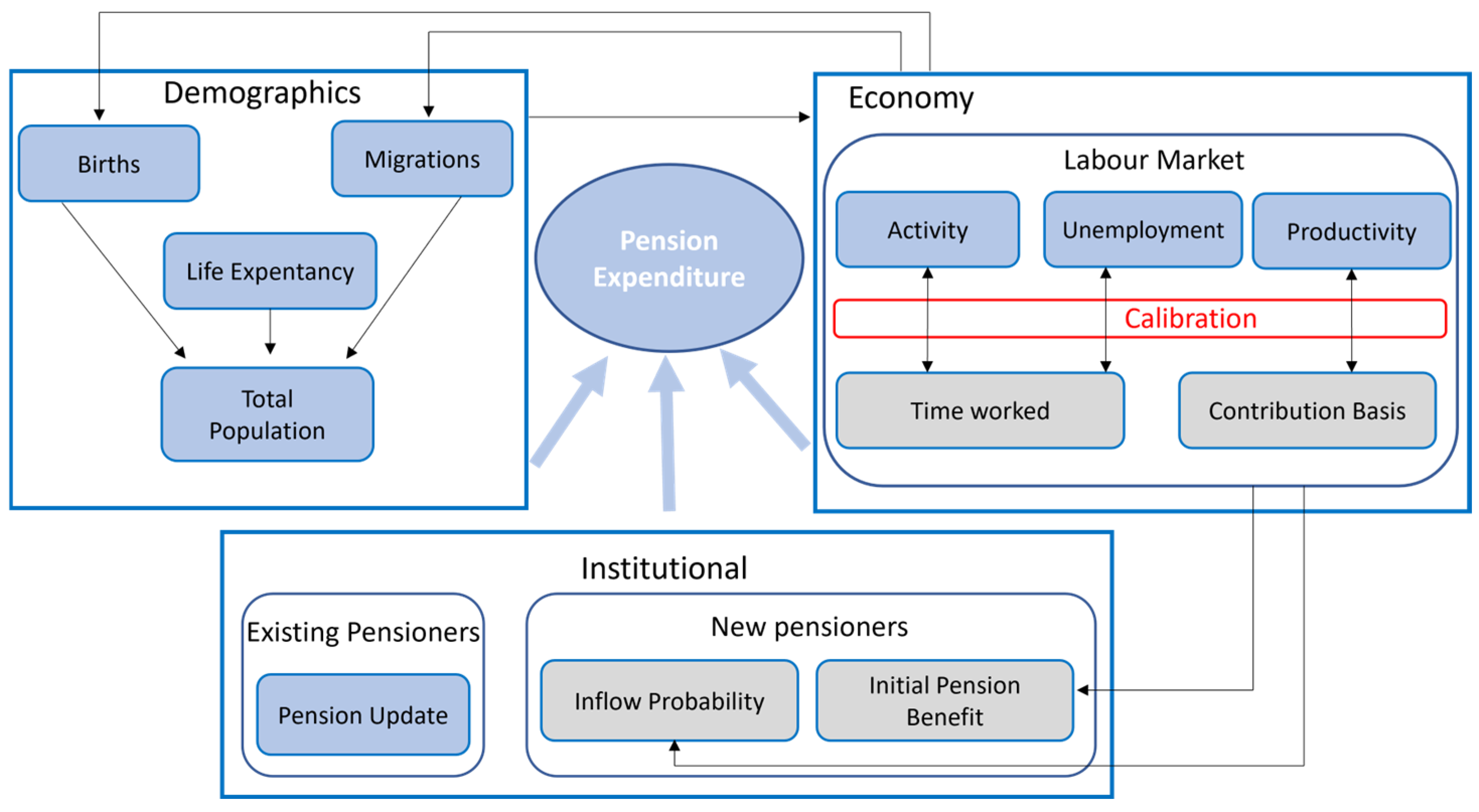
Figure 1 illustrates the simulation structure employed in this study, which enables the simultaneous analysis of the sustainability and adequacy of the social security contributory pension system. To project pension expenditures up to the year 2060, and to evaluate their adequacy with a focus on gender, three key factors are considered:
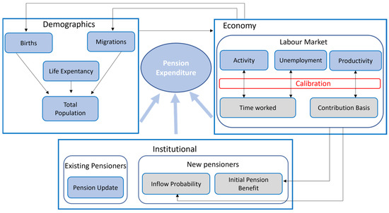
Figure 1.
Diagram of the hybrid pension simulation model.
- Demographic Evolution: This is determined by three components: births, net migration flows, and life expectancy. Births and migration are particularly influenced by the economic context.
- Economic Dynamics: These determine the state of the labor market, where factors such as the activity rate, unemployment level, productivity, and Gross Domestic Product (GDP) are crucial. These economic indicators are, in turn, influenced by demographic trends, particularly those affecting the working-age population.
- Institutional Environment: This includes the current legislation and any changes or modifications to it. These regulations affect existing pensioners through pension revaluation and new pensioners, impacting both the calculation of initial pension and eligibility to become a pensioner.
To integrate these three modules, a hybrid or mixed model has been adopted, implemented using the SAS code, which merges a macro approach and a micro approach. The macro approach, highlighted in blue in Figure 1, is predominantly applied in the demographic and labor market/economy modules. Conversely, the micro approach, indicated in gray, is used in the labor market module and in estimating variables affecting new pensioners. Since both approaches are employed within the labor market module, calibration of the estimates is essential in certain scenarios to ensure consistency. Calibration is performed from top to bottom, for example, for each individual, the probability of being employed is calculated based on their characteristics. Then, using the macro-level unemployment rate, individuals with the highest probabilities are selected as employed. This process facilitates the calibration between the micro approach and macro-level data, enabling the validation of results.
3.2. Data
The datasets used in this study are sourced from multiple providers, all of which are European or Spanish public institutions. These sources are described below, categorized by whether they supply macro-level aggregated data or individual-level micro data.
3.2.1. Macro Data: Demographic and Macroeconomic Scenario
This section outlines the demographic and labor market modules and dataset, which, in their central scenario, adhere to the core assumptions and data from the projections by Eurostat and the European Commission’s Ageing Working Group (AWG) (European Commission, 2017). This approach is categorized as “macro”, with a significant level of disaggregation. Data are detailed by age, sex, and year, while variables such as Gross Domestic Product (GDP) or the Consumer Price Index (CPI) are provided as single annual values.
The baseline demographic scenario is based on EUROstat Population Projections (EUROPOP, Eurostat 2019). For Spain, these projections anticipate a gradual and moderate increase in the fertility rate, from 1.32 children per woman in 2013 to 1.55 by 2060, marking one of the lowest fertility rates globally. Additionally, the scenario predicts a significant rise in life expectancy at birth during the same period, increasing by 6 years for men and 4.8 years for women, reaching 85.5 and 90 years, respectively, by 2060. However, the recent COVID-19 pandemic has prompted a slight downward revision of these projections, reducing expected life spans by approximately one year. Eurostat projects that the negative net migration balance observed in Spain in recent years—approximately 100,000 people in 2014—will gradually diminish and reverse starting in 2025, following an upward path that peaks at around 300,000 net inflows by 2050 and declines smoothly for the remainder of the period.
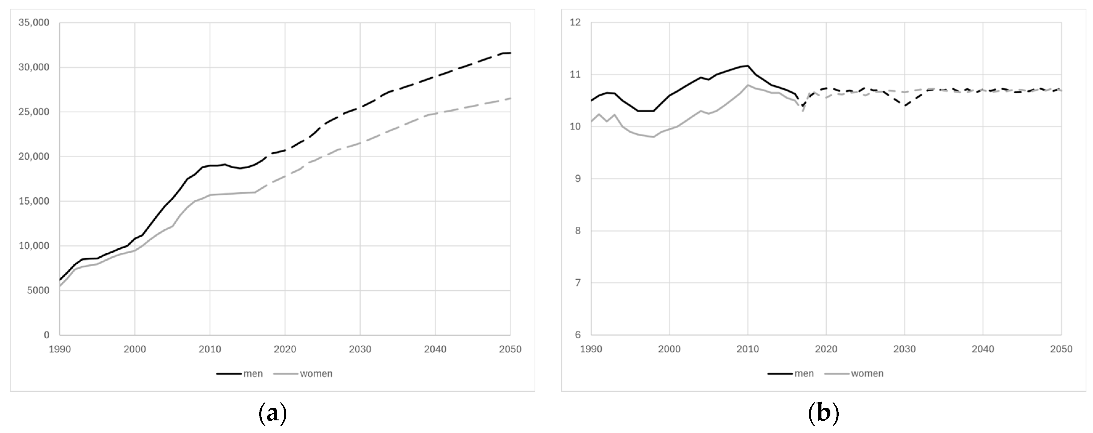
According to Eurostat’s estimates, population growth is projected until the late 2040s, followed by a gradual decline to approximately 47 million inhabitants, a figure slightly higher than at the beginning of the projection period. In addition to this inverted U-shaped trend, another significant outcome is the aging of Spanish society, as illustrated in Figure 2. The percentage of the population over 65 years of age is expected to increase until 2050, with slightly higher values for women due to their longer life expectancy.
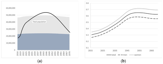
Figure 2.
(a) Expected evolution of the total population of Spain (women—blue, and men—gray); (b) elderly dependency ratio (by gender) [40].
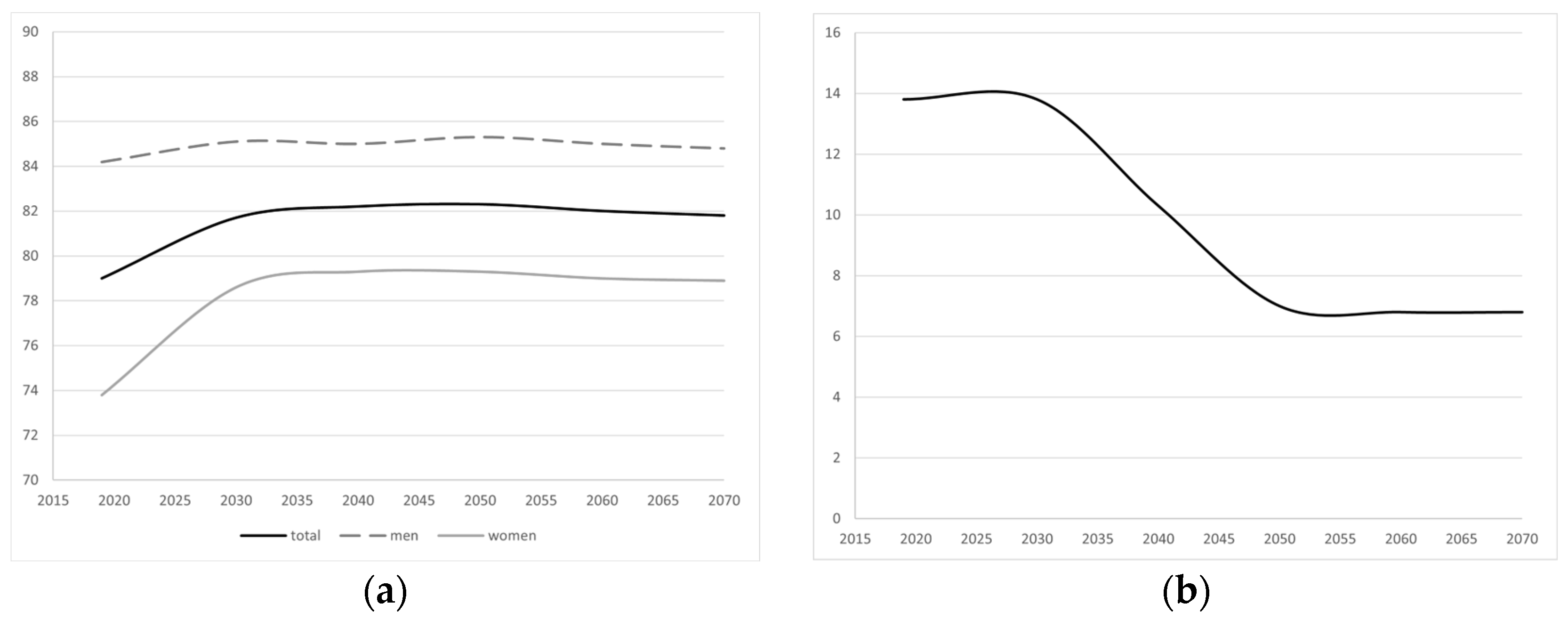
For the labor market variables, the projected evolution of the activity rate, differentiated by gender, along with the unemployment rate through 2070, is illustrated in Figure 3.
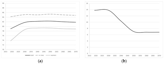
Figure 3.
(a) Evolution of the activity rate (by gender); (b) unemployment rate. Period 2018–2070 [1].
Furthermore, concerning other macroeconomic variables, it is projected that both the GDP deflator and the CPI will converge to a rate of 1.8% by 2025 and will remain constant for the rest of the projection period.
3.2.2. Micro Data: Individual Working Life
As shown in Figure 1, the micro approach is primarily applied during two phases. Initially, it involves the individual projection of key characteristics of a person’s working life. Subsequently, using this information, the initial retirement pension for new pensioners is calculated, mimicking the social security calculations. These calculations are performed using the MCVL (Continuous Sample of Working Lives), a dataset composed of anonymized individual-level microdata extracted from social security records.
The administrative file comprises a 4% sample of individuals from the reference population, which includes over 25 million people who have had some type of economic interaction with social security during a particular year. These interactions involve making contributions—either through employment or contributory unemployment—or receiving some type of contributory benefit, such as retirement, disability, widowhood, orphanhood, or benefits for family members. Consequently, each year, the MCVL contains information on approximately 1 million people.
In various files, the MCVL provides retrospective information on the following:
- Individuals: For each person selected in the sample, details such as date of birth, gender, country of birth, nationality, autonomous regions, and more are reported.
- Contribution base: For each individual and year, information is provided on the monthly and annual contribution base. Data are available from 1980 onwards.
- Affiliation: Displays all contracts held by each person selected in the MCVL throughout their working life, with details on the start date, type of labor relationship, part-time/full-time status, type of contract, etc.
- Pensions/benefits: Reflects the contributory benefits received by individuals, highlighting key details such as the type of benefit (retirement, widowhood, disability, etc.), the date of recognition, revaluation, and more.
Previously, with retrospective information up to the base year provided by the MCVL, estimates are obtained with a high level of disaggregation on labor market participation, days worked in the year, or the annual contribution base, which will subsequently be used in the projection.
Using the 2016 MCVL file, individuals who are not receiving a pension and are thus considered active at the end of 2016 are selected. The most important labor-related variables for each of these individuals are then projected up to 2060.
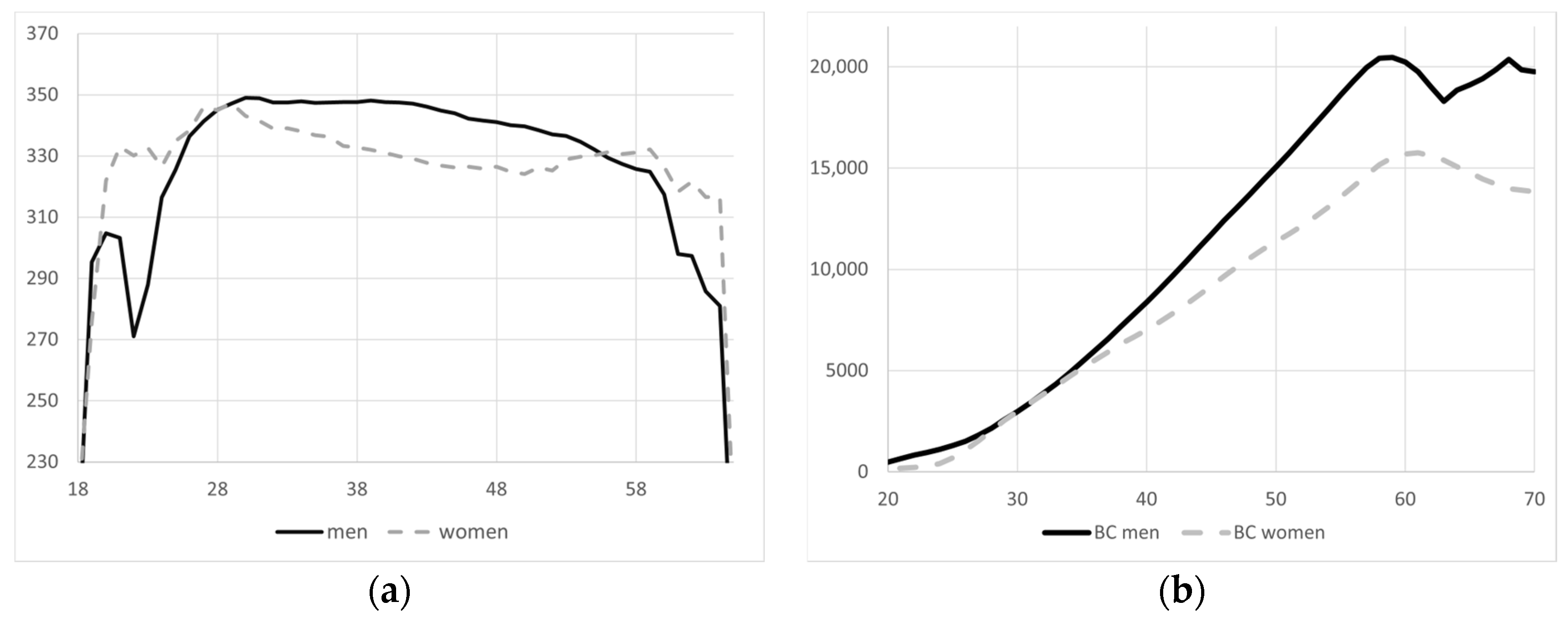
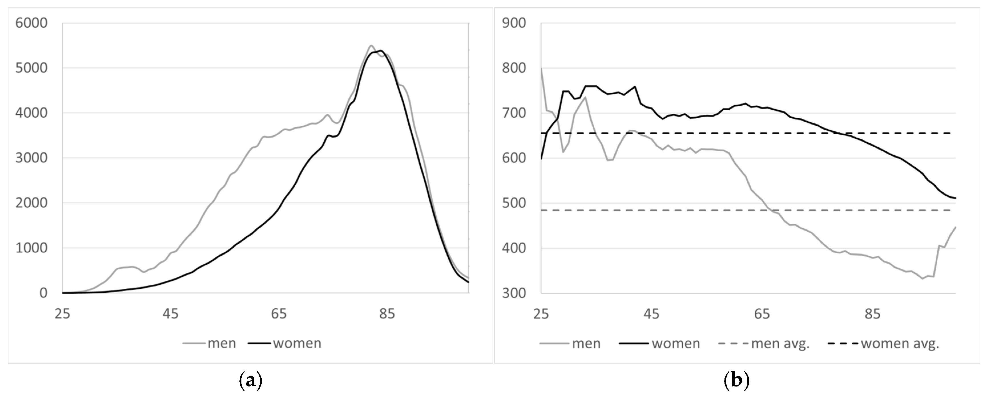
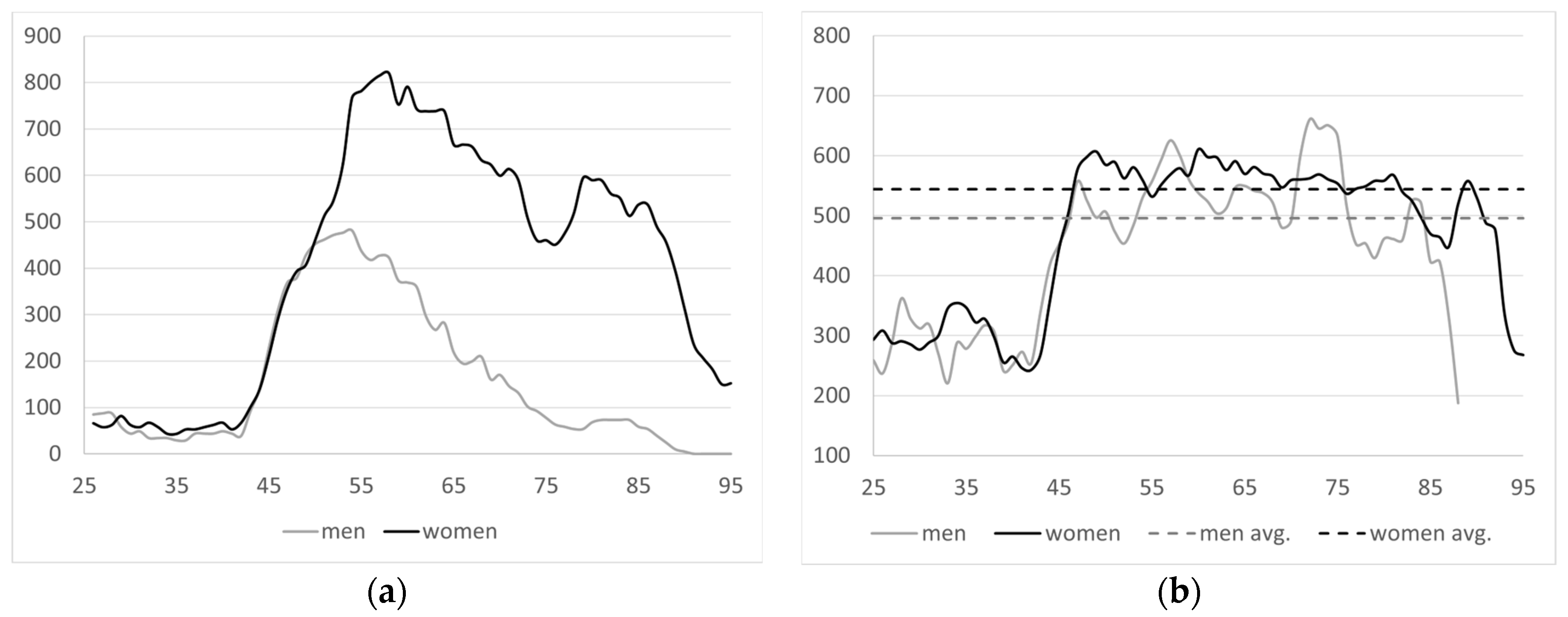
As previously indicated, due to the high level of disaggregation of the information offered in the MCVL, it is possible to obtain estimations with a high level of detail. Figure 4 shows, using the MCVL affiliation information, the days worked according to the age and gender of the selected individuals, as well as the average annual contribution base of the workers by age and gender.
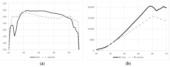
Figure 4.
(a) Number of days worked per year by age; (b) average annual contribution base by age and gender [41].
With this retrospective information, it is possible to generate data on the time worked or wages that will be used later in the projection and simulation. Figure 4a,b illustrate the time worked as well as the evolution of the contributory base for retired persons between 2014 and 2016, differentiated by gender.
Using these calculations and considering 2016 as the baseline, projections are individually made for the active population of that year, determining whether they are employed or not, the number of days worked per year, and the annual contribution base until the year 2060 or until the individual reaches the age of 75. These projections are based on socio-demographic variables such as gender, age, educational level, and GDP growth. Figure 5a,b display the average values of the contribution base and months worked, categorized by gender and year, derived from the aggregation of individual data from the previously conducted micro projection.
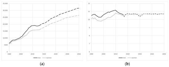
Figure 5.
(a) Average annual contribution base by gender and year; (b) months worked by gender and year. Observed values (solid line) and projected values (dotted line) [41].
This approach facilitates a deeper understanding of how demographic and economic factors interact to shape future labor market outcomes and pension contributions.
3.3. Contributory Pension System Projection
Contributory pensions are economic benefits, typically indefinite, granted to beneficiaries who have had a prior legal relationship with the social security system and meet specific requirements depending on the type of pension. The amount of the pension is determined based on contributions made by the worker and the employer during the period considered for calculating the pension’s regulatory base.
The types of contributory pensions include the following:
- Retirement: A lifelong economic benefit granted to workers who cease employment due to age or reduce their working hours and salary as legally established.
- Permanent disability: Covers the loss of wages or professional income suffered by an individual affected by a pathological or traumatic process that reduces or nullifies their working capacity. It can be partial, total, absolute, or involve major disability.
- Survivorship: These benefits are designed to compensate for the economic need caused by the death of certain individuals. They are classified as widowhood, orphanhood, and family allowance.
This section presents the projection methodology for the five types of contributory pensions: retirement, widowhood, disability, orphanhood, and family allowance. The methodology differs between retirement pensions and the other four types. For retirement pensions, a purely micro approach is employed using the MCVL from social security. This micro method generates individual-level values for working time and salaries, enabling the estimation of potential annual pensions for each person under existing legislation. These micro estimates are then aggregated to obtain macro-level indicators, such as the average initial pension.
For the other four types of contributory pensions (widowhood, disability, orphanhood, and family allowance), a more macro projection method is applied. Instead of micro-level calculations, projections are performed at the level of a “representative agent” by age and gender. These values are derived from social security statistics (e.g., average pension by age and gender) and data from the Spanish Statistics Office (INE) (e.g., population, mortality rates).
This section outlines the main features of the pension model, which projects key expenditure variables disaggregated by age, gender, and year for the four contributory pensions mentioned (widowhood, disability, orphanhood and family allowance). The projection of retirement pensions will be developed in greater detail in the next section.
- Projection Model
The projection proposal will enable the estimation of total pension expenditure for the analysis of the system’s sustainability, in addition to the average pension by gender and age group, which provides information on adequacy while incorporating the gender component.
Total pension expenditure in year t () is calculated using information disaggregated by gender and age and can be expressed as follows:
where j refers to the type of contributory pensions considered (j = 1,…,5 relating to retirement, widowhood, disability, orphanhood and family allowances), s is related to gender (s = 1,2 for male and female), and e for age, while is the average annual pension of pension type j, for gender s and age e, and is the number of pensions in that year for the same breakdown as above.
- Number of pensions by gender and age
As regards the evolution in the number of pensions, a stock value, , is considered along with annual inflow and outflow values.
With regard to pension inflows, referred to as , a separate analysis will be made for the calculation method of each type of contributory pension in the relevant section, whereas the number of outflows in year t for a given age and gender is obtained on the basis of the mortality rate, either from the Spanish Statistics Office (INE 2018) or Eurostat, as , as follows:
where is the number of existing pensions for age e in year t−1.
The total number of pensions in a year is obtained from the pensions of the previous year, together with the evolution of the inflows and outflows in that year.
- Average pension by gender and age
The other element that must be calculated is the pension for each contributory pension type, indicated by . The initial pension for new pensioners, denoted as , will be described in each of the different sections below. The final average pension for the outflows for each age and gender, referred to as , is calculated as the weighted average of the number of existing pensions from individuals one year younger in the previous year, revalued that year (called ), and the number of new pensions in the year, so that
where 1/2 is used to specify that the year’s inflows are evenly distributed throughout the year.
Finally, the average pension for each type of retirement, by age and gender, as the mean of the different pensions calculated above, is determined using the following formula:
The main characteristics of each of the several types of contributory pensions are detailed below. To this end, for each type of pension, firstly, the number of pensions and average pension benefit by age and gender in the baseline year are shown, which will be taken as the starting values in the projection. Then, different estimation methods are proposed for the most relevant variables in each case (initial pension, number of inflows, etc.), which will be necessary to project these variables regarding the benefit amount and the number of pensions.
3.3.1. Widowhood Pension
- Number of pensions and average pensions in the baseline year by gender
Using the baseline information, the figures below show the total number of widowhood pensions per age and gender, as well as the existing average pension, which are considered the starting values for the projection. In 2016, there were a total of 2,180,666 female widowhood pensioners receiving an average monthly pension of EUR 655, and 178,385 male widowhood pensioners receiving an average monthly pension of EUR 484. Based on this stock, for the baseline year, the projected number of pensions, , and average pension amount, , are shown in Figure 6.

Figure 6.
(a) Number of widowhood pensions per age and gender in baseline year; (b) average pension per age and gender in baseline year [41].
- Number of inflows
The number of new widowhood pensions in a certain projected year is calculated by multiplying the population for that year by the probability of receiving a widowhood pension for each gender s calculated in the baseline, which remains constant over the entire projection period.
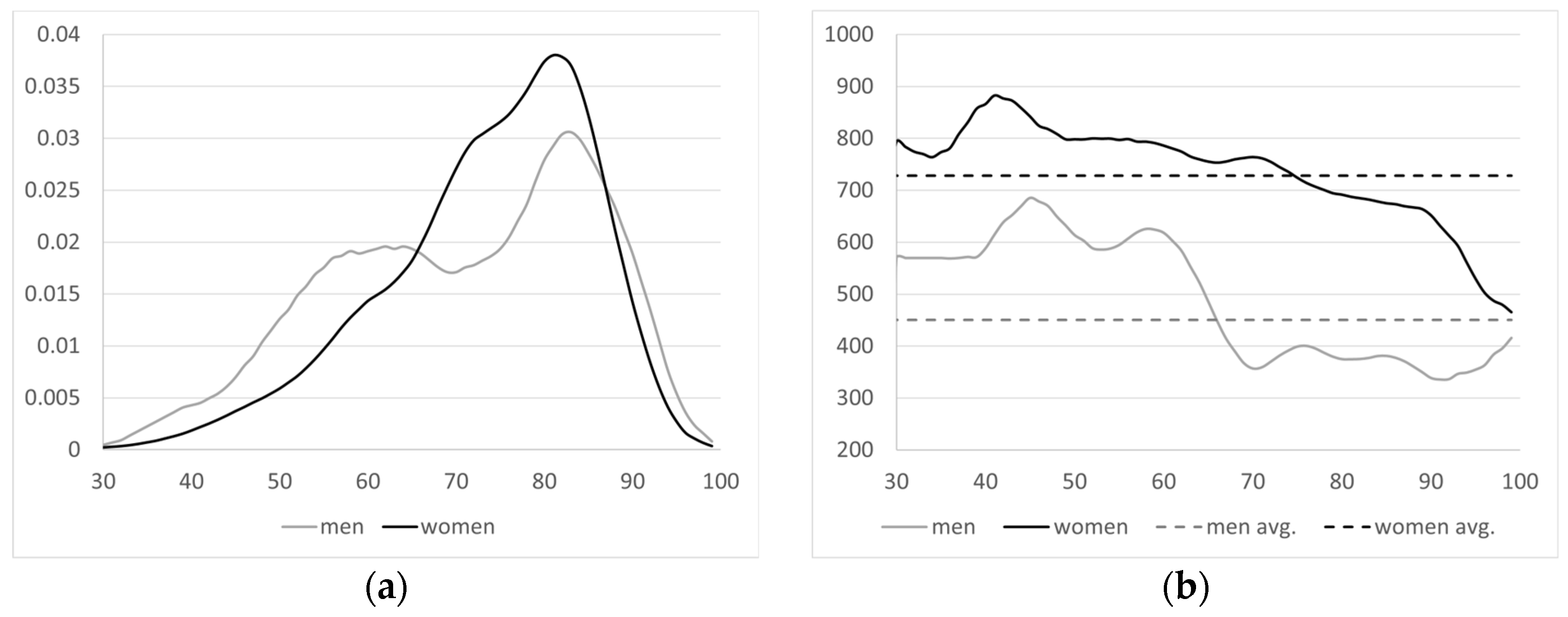
Figure 7 shows for each gender.
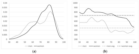
Figure 7.
(a) Density function of widowhood inflows in the baseline year by age and gender; (b) average initial pension in the baseline year by age and gender [41].
The probability of widowhood inflows is calculated by dividing the number of new widowhood pensions by age and gender in the baseline year by the existing population in that year:
This is shown in Figure 7a. The number of pension outflows and the total widowhood is not significant compared to the standard estimate.
- Initial Pension
The initial widowhood pension is calculated as shown below. The initial pension in the baseline year is calculated for each gender and age as shown in Figure 7b. This information is used to determine the differential between the initial pension for a certain age and gender and the mean initial pension for that gender, so that
where is the average initial pension in the baseline year for s.
Next, the fact that new widowhood pensions must result from an outflow from the system due to the death of the decedent, an individual of the opposite sex who was an active worker , retired, , or permanently disabled , must be considered. Therefore, the basis on which to calculate the widowhood benefit in year t is the mean income of each of the three options considered:
where , and are the different incomes in employment, retirement and disability situations of the decedent in the previous year. Once this value is established, it is compared with the sum from the previous year to determine the increase over the year. This amount is used to calculate the starting pension for a certain gender, as follows:
Next, to disaggregate this amount by age, the initial widowhood pension for a certain year is calculated for the different ages and genders as follows:
To calculate the final pension and average pension, the standard method indicated in the previous section is used.
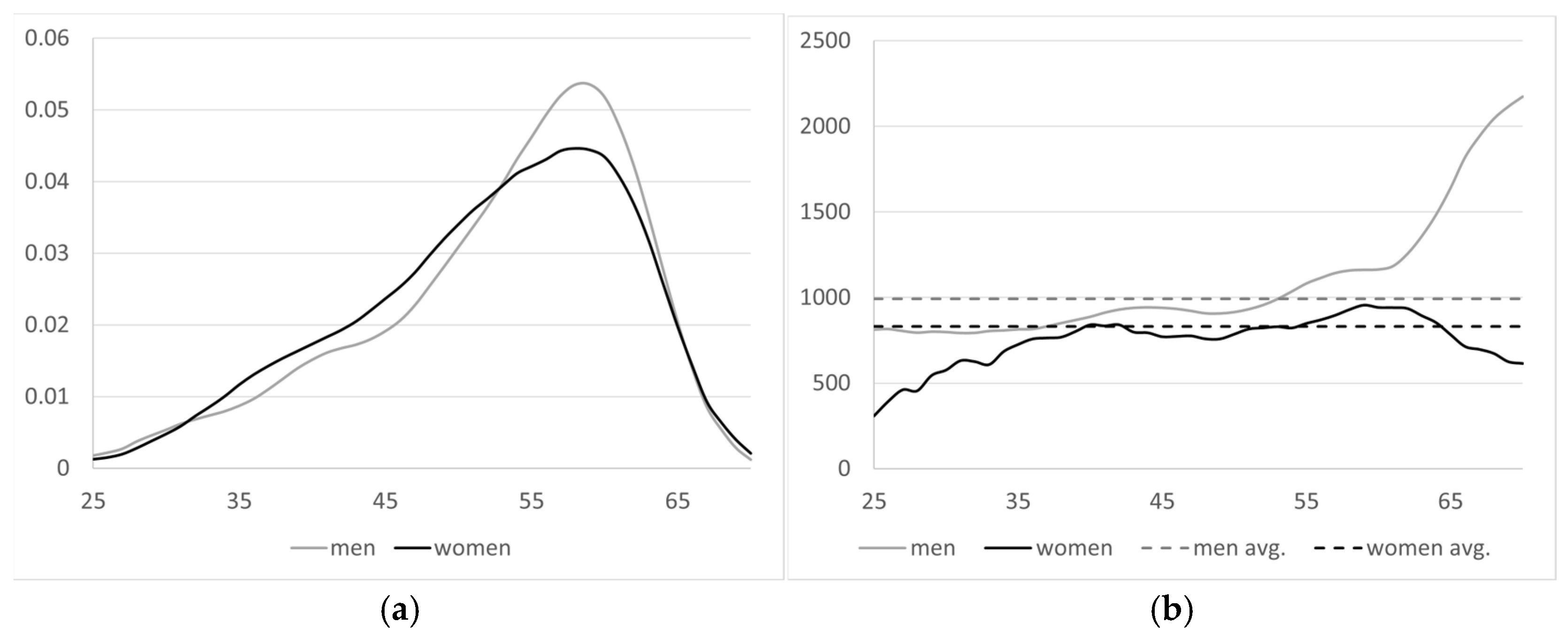
3.3.2. Disability Pension
- Number of pensions and average pensions in the baseline year by gender
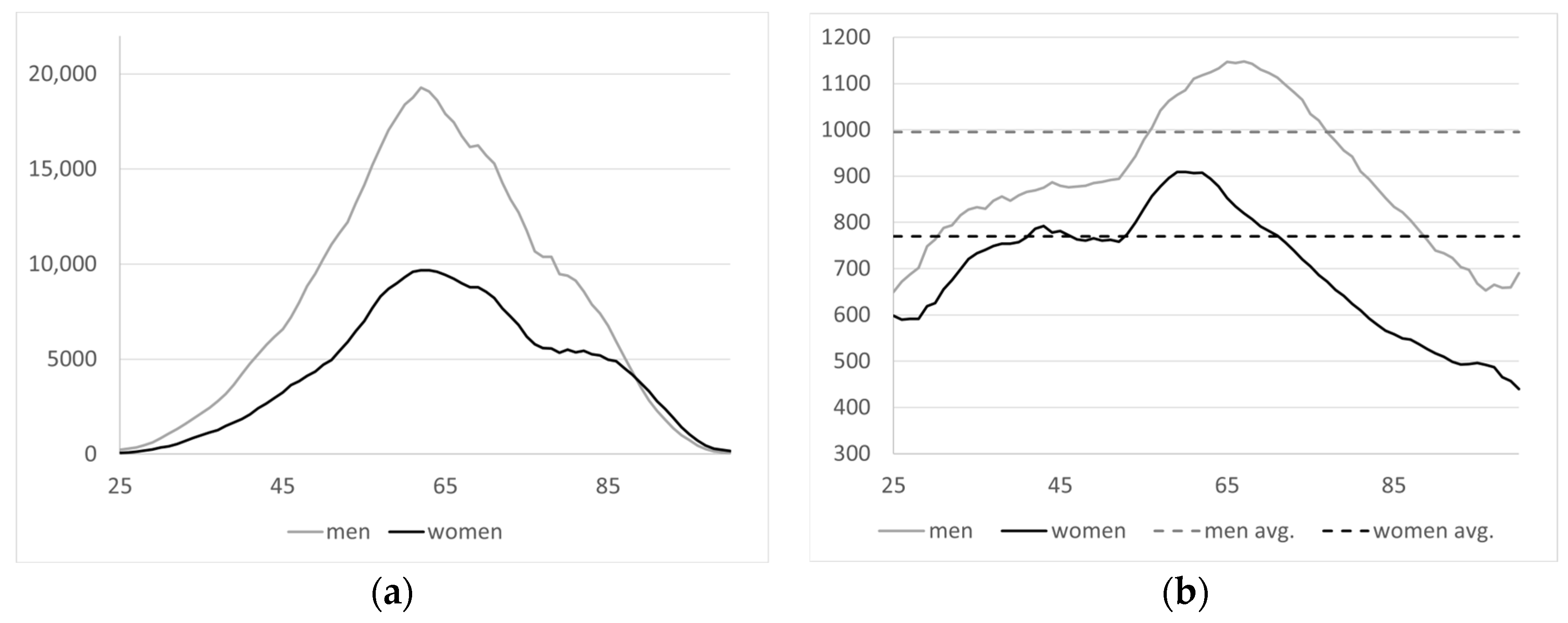
For the baseline year, Figure 8 shows the total number of disability pensions by age and gender, as well as the existing average pension for the different stocks considered at the start of the projection.
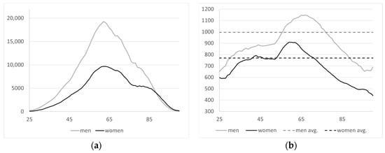
Figure 8.
(a) Number of disability pensions by age and gender in baseline year; (b) average pension by age and gender in baseline year [41].
For the baseline year, there were 333,521 female disability pensioners receiving an average monthly pension of EUR 800, and 609,628 male pensioners receiving an average monthly pension of EUR 995. Using these baseline year values, the projected number of pensions, , and the average pension, , are calculated according to the following expressions.
- Number of inflows
The number of new disability pensions is calculated by multiplying the working population by the probability of becoming disabled for each gender s calculated in the baseline year, which remains constant over the entire projection period.
The probability of becoming disabled is calculated by dividing the total disabilities for one gender by the working population of that gender in the year for the baseline year:
Once the total number of disabilities by gender has been established for a certain year, this figure is disaggregated for different ages using the density function calculated in the baseline year, which is constant throughout the projection period.
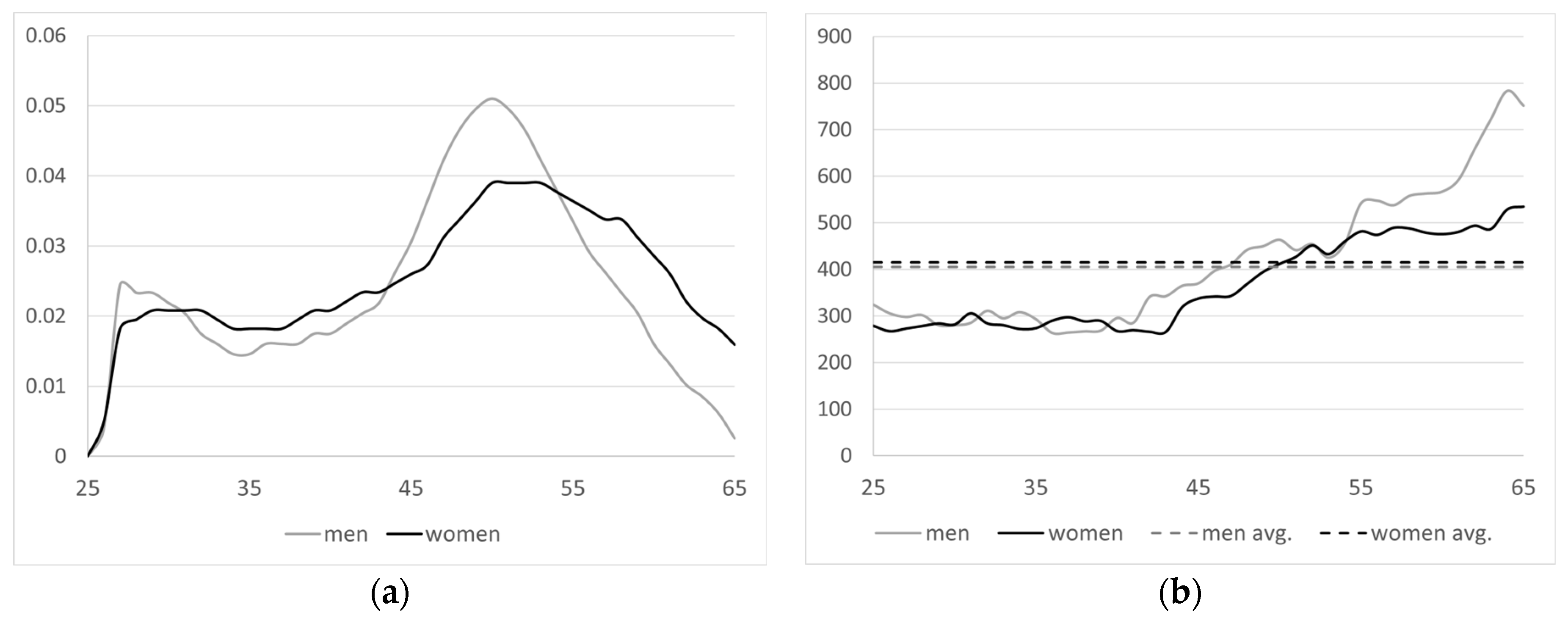
The density function for each gender is calculated for the baseline year by dividing the disability inflows for a certain age by the total number of inflows of that gender, as shown in Figure 9.
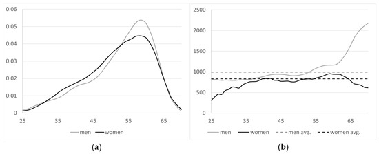
Figure 9.
(a) Density function of disability inflows in the baseline year according to age—by gender; (b) starting disability pension in the baseline year according to age—by gender [41].
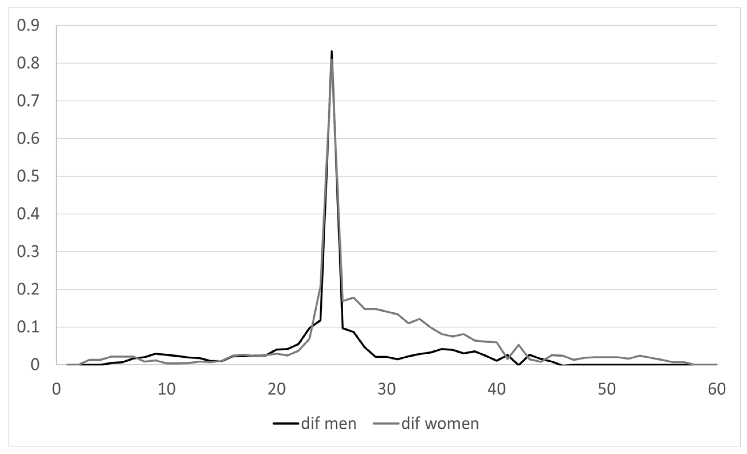
- Number of outflows
Given the unique characteristics of these pensions, the profile for disability outflows differs somewhat from that of the rest of the population. Figure 10a shows the probability of disability pension outflows for the baseline year according to data from the MCVL in comparison with the mortality rate provided by the INE for the Spanish population in that baseline year. Figure 10b depicts the mortality differential between the two series, which is
where refers to the disability pension outflow rate derived from MCVL data, whereas is the outflow rate linked to mortality calculated by the INE for the entire population that year.
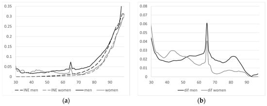
Figure 10.
(a) Disability outflow rate according to MCVL and outflows linked to mortality based on INE tables in baseline year, by age and gender; (b) series in the baseline year, by age and gender [41,42].
Using this series, the estimated number of outflows for any year in the projection period is calculated as follows: the outflow rate is initially estimated for a certain year by combining the mortality rate published by an official agency (INE or EUROSTAT)—known as —with the excess mortality previously obtained in the baseline year.
Outflows for a certain year are determined by applying this outflow rate to the sum of pensions from the previous year and new pensions added that year:
- Initial pension
The initial disability pension is linked to the wages of a worker who experiences an accident or illness. The initial pension for a specific gender and year, , is determined as the starting pension from the previous year, increased in the same proportion as the wages (contribution base, ) increase between those two years.
being . After calculating the increase in the mean initial pension, the pension for each age is then determined by using the differential found in the mean initial pension by age for each gender in the baseline year, obtained in Figure 9.
where the differential is calculated as , in which is the initial disability pension for each gender in the baseline year.
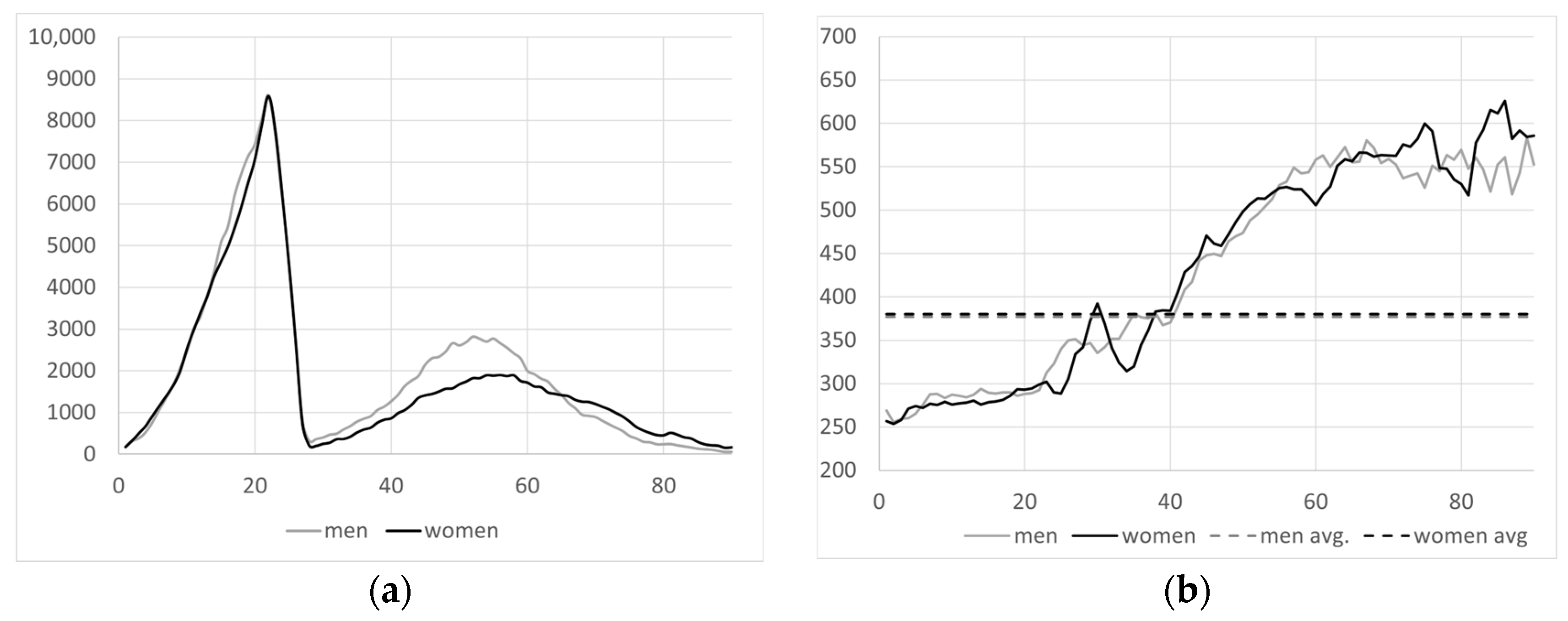
3.3.3. Orphanhood Pension
- Number of pensions and average pensions in the baseline year by gender
Using the MCVL data, Figure 11 shows the total number of orphanhood pensions by age and gender, , as well as the existing average pension, , which are considered the starting values for the projection.

Figure 11.
(a) Number of orphanhood pensions by age and gender in baseline year; (b) average pension by age and gender in baseline year [41].
For the baseline year, there were 161,344 female orphanhood pensioners receiving an average monthly pension of EUR 377, and 177,177 male pensioners receiving an average monthly benefit of EUR 377. Based on these starting figures, the projection up to 2060 is carried out as indicated below.
- Number of inflows
The number of new orphanhood pensions in a certain projected year, is calculated by multiplying the population for that year, , by the probability of starting to receive an orphanhood pension for each gender s calculated in the baseline year, which remains constant over the entire projection period.
Figure 12 shows for each gender.
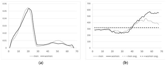
Figure 12.
(a) Density function of orphanhood inflows in the baseline year by age and gender; (b) average initial pension in the baseline year by age and gender [41].
The probability of new orphanhood pensions is calculated by dividing the number of new orphanhood pensions by age and gender in the baseline year by the existing population in that year:
This is shown in Figure 12a.
- Number of outflows
Similar to the case of disability pensions, orphanhood pensions have certain unique features. Figure 13 shows the difference between the orphanhood outflow rate obtained from MCVL data in the baseline year, , and the mortality rate provided by INE for that same year. Therefore, the figure depicts the following:
where was already defined as the outflow rate linked exclusively to the INE mortality tables.
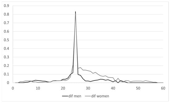
Figure 13.
in the baseline year by age and gender [41,42].
Next, the orphanhood outflow rate series is calculated for a certain projection year as the sum of the mortality rate published by INE or Eurostat, , and the outflow differential for this population group as calculated above:
Thus, orphanhood outflows are determined as follows:
where is the total number of orphanhood pensions by age and gender in the previous period. The total number of orphanhood pensions does not differ substantially from the standard estimation method.
- Initial pension
The initial orphanhood pension is calculated as shown below. The starting pension in the baseline year, , is initially calculated for each gender and age, as shown in Figure 12b. This information is used to determine the differential between the initial pensions:
where is the average initial pension in the baseline year for gender s.
Next, new orphanhood pensions, , must result from an outflow from the system due to the death of the decedent, an individual who was an active worker, , retired, , or permanently disabled . Therefore, the basis for calculating the orphanhood benefit in year t is the mean income of each of the three options considered:
Once this value has been obtained and compared with the amount in the previous year, the increase over the year is calculated. Using this amount, the initial pension for a given gender is obtained as follows:
Next, to disaggregate this amount by age, the initial orphanhood pension for a certain year is calculated for the different ages and genders as follows:
To calculate the outflow pensions, the final number of orphanhood pensions and average pension, the standard method indicated in the previous section is used.
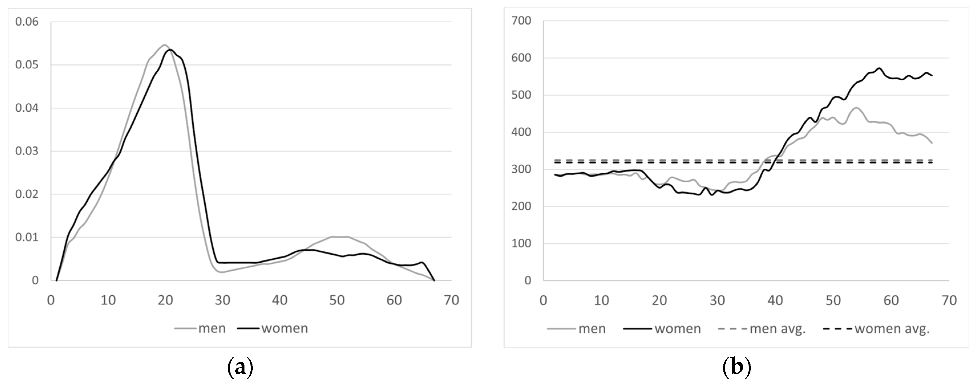
3.3.4. Family Allowance Pension
- Number of pensions and average pensions in the baseline year by gender
For the baseline year, Figure 14 shows the total number of family allowance pensions by age and gender, , as well as the existing average pension, , which are the figures used to start the projection.
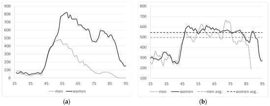
Figure 14.
(a) Number of family allowance pensions by age and gender in baseline year; (b) average pension by age and gender in baseline year [41].
There were 28,914 female family allowance pensioners receiving an average monthly pension of EUR 544, and 11,338 male pensioners receiving an average monthly pension of EUR 496.
- Number of inflows
The number of new family allowance pensions is calculated in a manner similar to that of orphanhood. The number of inflows is calculated by multiplying the population for that year, , by the probability of receiving a family allowance pension for each gender s calculated in the baseline year, which remains constant over the entire projection period.
Figure 15 shows the for each gender. This probability is calculated by dividing the number of new family allowance pensions by age and gender in the baseline year, , by the existing population in that year:
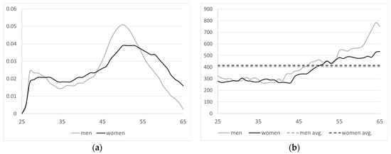
Figure 15.
(a) Density function of family allowance inflows in the baseline year by age and gender—; (b) average initial pension in the baseline year by age and gender [41].
- Initial pension
As is the case with orphanhood, the growth rate between two years for the average family allowance pension is determined as follows:
where was defined previously. After obtaining this value, Figure 15a is used to disaggregate by age, so that
and . The projection for retirement pensions is described below.
To calculate the outflow pensions, the final number of family allowance pensions and average pension, the standard method indicated in the previous section is used.
3.3.5. Retirement Pension
- Spanish Retirement pension and the Implementation of 2011 Reform
The public pay-as-you-go pension system is based on the principle of intergenerational solidarity, meaning that active workers finance the benefits of those receiving a pension. The main source of funding for the contributory pension system is the social contributions made by employers and employees as a percentage of the contribution base, limited by certain caps and minimums on earnings. System expenditures are generated by the payment of retirement benefits. A retirement pension is a financial benefit granted once the established age is reached, to individuals who fully or partially cease to perform the activity under which they were included in the social security system and can prove that they fulfilled the set contribution period (there are several types of retirement: ordinary, partial, flexible and early). Prior to the 2011 reform, the main requirement for receiving a retirement pension was to have made social security contributions for at least 15 years, with at least 2 years being within the last 15 years before the statutory retirement age. Once the pensioner’s right to receive this benefit has been acknowledged, the starting benefit received, also known as the initial pension, depends on the retirement age (65 years old to receive 100% of the pension), the number of years of contributions (35 years to receive 100% of the pension sum) and the earnings (contribution bases) over the previous 15 years. It is calculated as follows:
This method of calculating the retirement pension is based on the income earned by the future pensioner in the years prior to retiring. Therefore, the benefit, referred to as , is calculated as the regulatory base (BR) multiplied by the reduction factor, , which depends on the number of years worked, and another factor,, which depends on the retirement age. Using the formula shown in the equation above, each of the quantities indicated in the formula must be developed, starting with the BR for a person who retires in the year t:
Therefore, BR is the mean contribution base over the last 15 years, where the amount, is the contribution base of year i, and the variable is the inflation rate in year i. This contribution base is essentially the annual income earned within the thresholds (the lower and upper limits depend on the worker’s job category). Contribution gaps are filled less generously than in the past. The most recent 48 months are calculated using the minimum contribution base, and all previous months are calculated using 50% of the minimum contribution base, instead of 100% of the minimum base.
There are two more elements needed to calculate , which are considered reduction factors: the first of these is related to the number of years in which contributions were paid, called n, with a minimum of 15 years of contributions required in order to be eligible to receive the pension. Its formula is as follows:
The second reduction factor in Equation (34) is related to the retirement age, as individuals below the age of 61, for the unemployed, and 63, for active workers, are not eligible. Early retirement in the event of dismissal (in the case of general early retirement, the minimum age for eligibility is 63 and the annual reduction coefficient is 7.5% per year in advance of the standard age) is structured as follows:
Once has been determined, certain maximum and minimum values stipulated by law each year are applied so that the benefit falls between these two amounts. The above refers to the calculation of new pensions in the system. Pensions already in the system will be updated according to the annual CPI.
The reform also aimed to balance the financial sustainability of the pension system by aligning benefit calculations with contribution periods. This approach reflects a broader trend in developed countries to adapt pension systems to increasing life expectancy and changing labor market dynamics. These adjustments were designed to ensure intergenerational equity while maintaining adequate income levels for pensioners.
Based on this regulatory framework in place at the beginning of 2010, the pension reform of 2011, which began to be implemented in 2013, essentially involved raising the statutory retirement age from 65 to 67, gradually extending the calculation of the regulatory base to 25 years, as well as the number of years required to receive 100% of the pension. Table 1 shows the rate of implementation of the reform, up to full implementation in 2027, for the most relevant parameters.

Table 1.
2011 Reform—evolution of the statutory retirement age, number of years for calculation of the BR and coefficient related to the minimum time worked to avoid penalization [41].
- Number of pensions and average pensions in the baseline year
For the baseline year 2016, Figure 16 shows the total number of retirement pensions by age and gender, as well as the existing average pension. These are the values that will be used to start the projection.
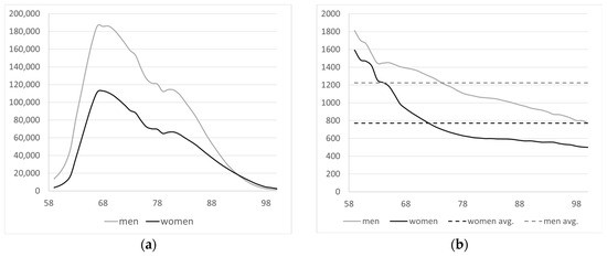
Figure 16.
(a) Number of retirement pensions by age and gender in baseline year; (b) average pension by age and gender in baseline year [41].
There were 2,125,985 female pensioners receiving an average monthly pension of EUR 756, and 3,605,892 male pensioners receiving an average monthly pension of EUR 1,211. Based on this volume of retirement pensioners, the way in which pension inflows are generated and the starting pension are described below.
- Initial retirement pension
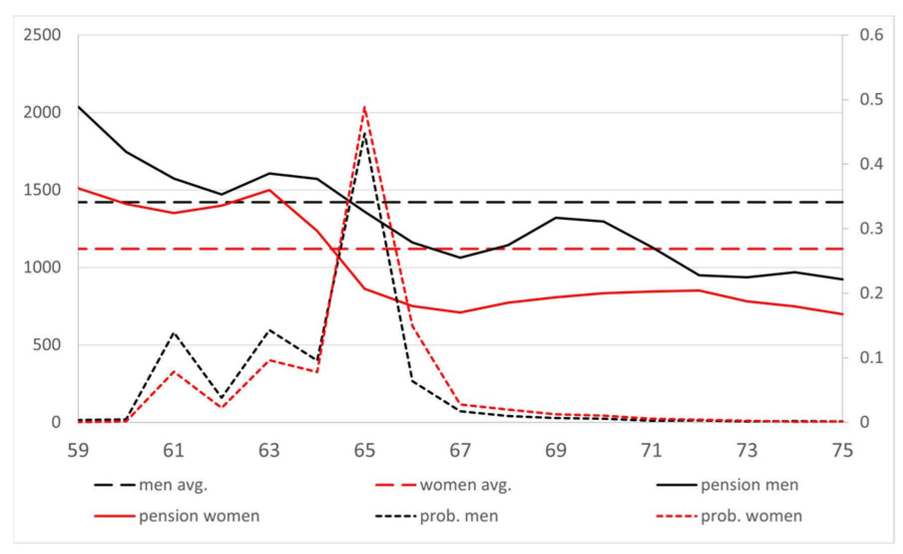
Figure 17 shows the average retirement pension by age and gender in the baseline year, as well as the proportion of individuals who retire that year. Higher initial pensions are observed for younger ages and a sustained difference in benefits is seen for the entire estimated age group. Regarding the projection years, individual employment history information is available up to 2060 or until the person reaches the age of 75. By applying the formulas indicated in the previous section for calculating the initial pension to each individual in each projection year, the individual starting pension is determined.

Figure 17.
Average pension (dashed line), pension by age (solid line), and proportion of retired individuals (dotted line) by age and gender in baseline year [41].
- Number of retirement inflows
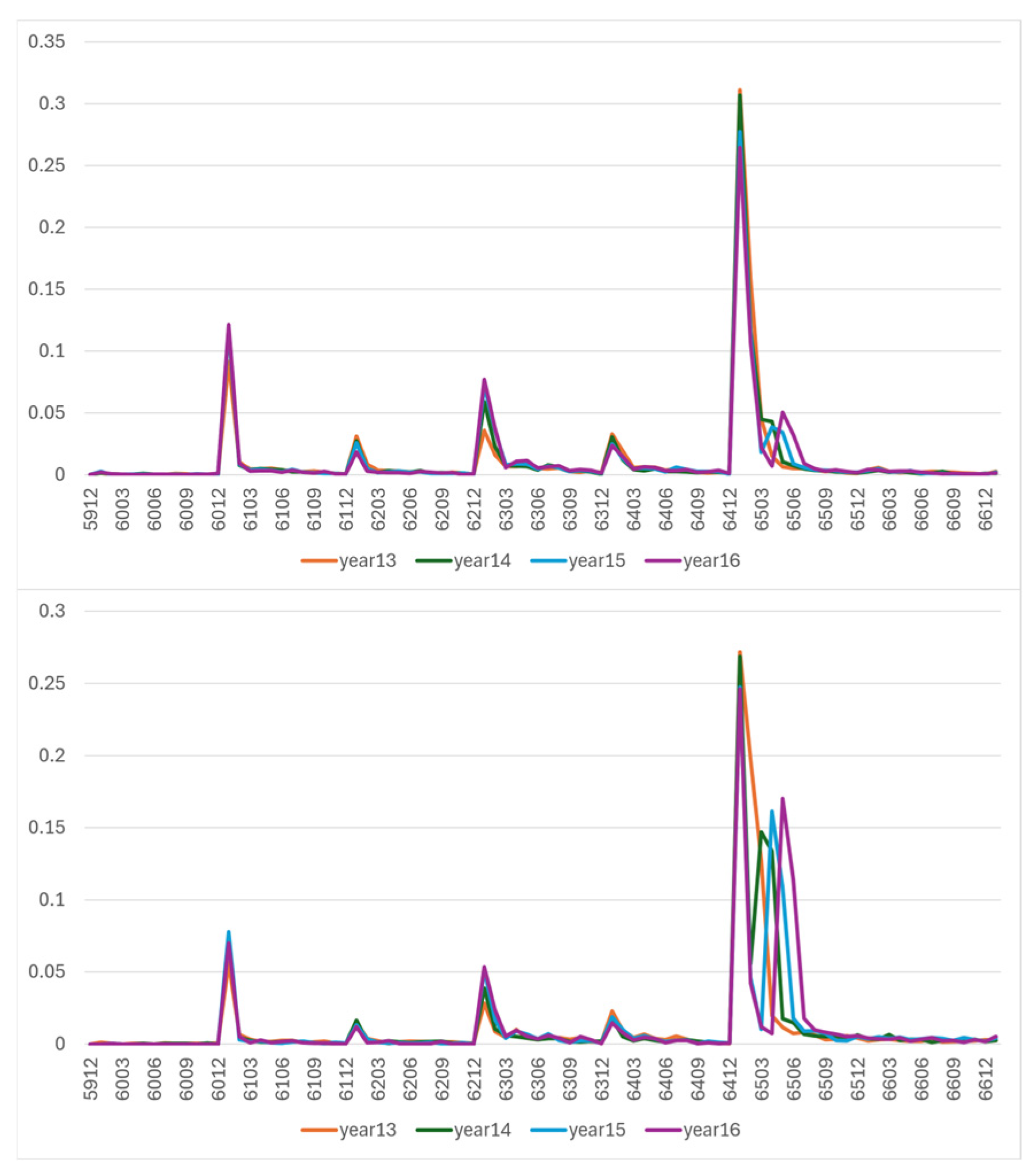
In terms of the starting retirement pensions, MCVL data have been used to calculate the effect that the 2011 reform is having on the behavior of monthly inflows (rather than at discrete ages as most simulators do), finding the behavior shown in Figure 18.
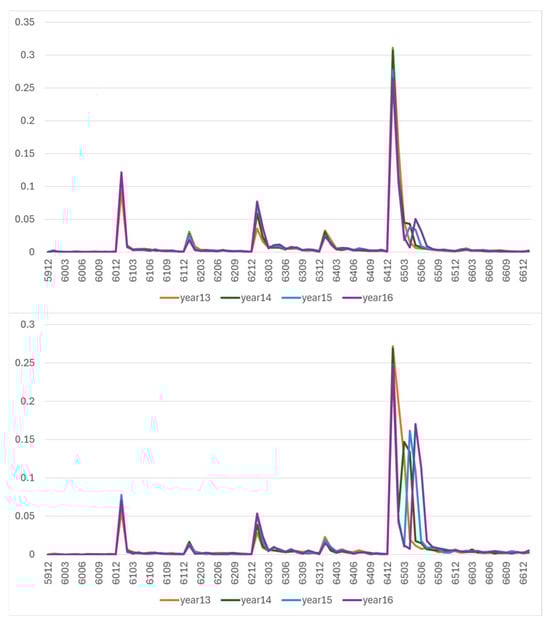
Figure 18.
Retirement inflows according to age and month over the past 4 years. Men (above) and women (below) [41].
As shown, the distribution of male inflows has not been altered by the introduction of the 2011 reform, with only a slight upturn in inflows at the age of 65 and 3 months in the last 2 years (2015 and 2016). However, the number of female inflows is much more sensitive to the implementation of the reform, as the minimum contribution period is not reached, which forces many women to delay their retirement as the statutory retirement age shifts.
This sensitive response to the implementation of the reform, in light of the inflows at the voluntary and statutory retirement age, is reflected in the projection of this model up to 2060.
4. Results
In this section, the simulation results are presented from both the sustainability and adequacy perspectives, with different levels of disaggregation in the estimations.
4.1. Sustainability of the Spanish Pension System
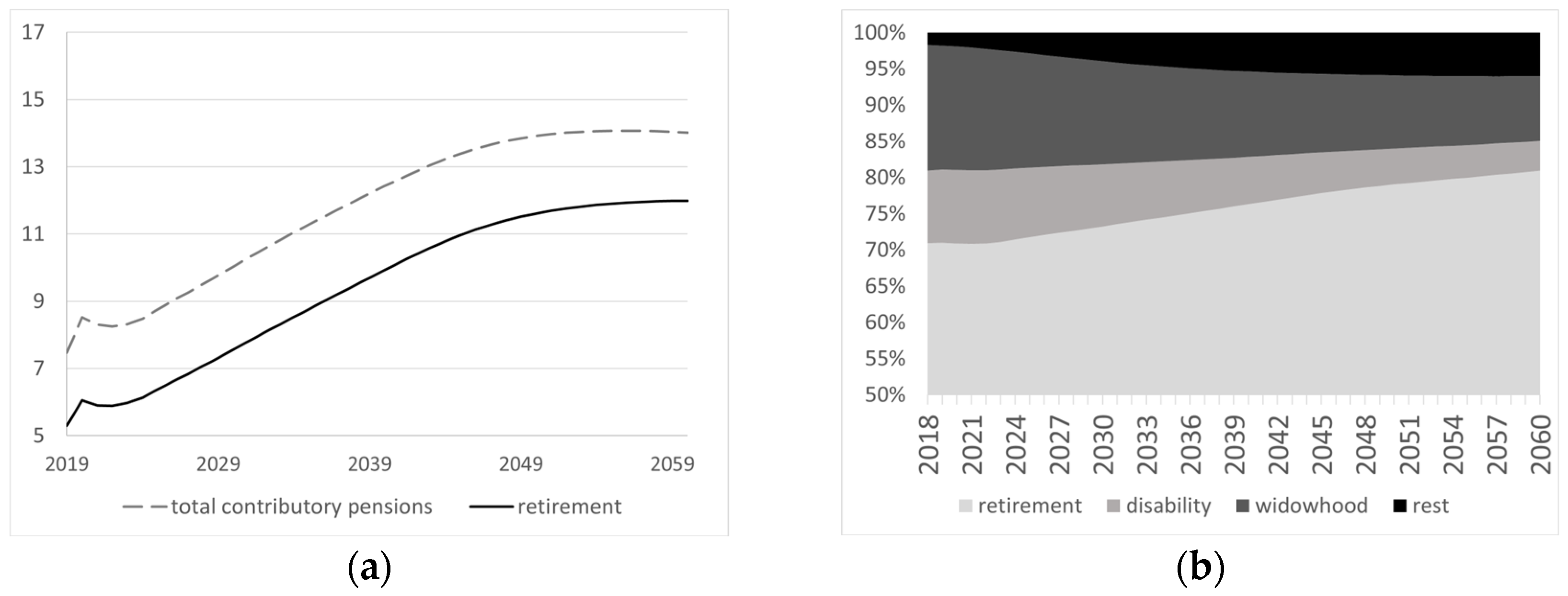
Regarding the sustainability of the contributory pension system, Figure 19 illustrates the evolution of pension expenditures as a percentage of GDP (Figure 19a), as well as the proportion of each pension type in total expenditures (Figure 19b).
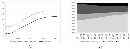
Figure 19.
(a) Expenditure on contributory pensions (and retirement); (b) percentage of total expenditure on contributory pensions for different pension types [41].
The COVID-19 crisis led to an increase in expenditure because of falling GDP, which later stabilized. Without the implementation of the 2013 reform, the trend suggests that pension expenditures would reach more than 13.9% of GDP (The estimated value of expenditure as a percentage of GDP falls within a range similar to that found in other studies conducted for Spain, such as [7], which reported a value of 13.5%, or Independent Authority for Fiscal Responsibility (AIReF), which found it to be 13.4%), a value similar to those reported in other studies, such as the Ageing Report 2018 by the European Commission (2018) estimated in 13.9 in 2030. This expenditure is expected to remain stable from the 2050s onward. Regarding the distribution of different components of this expenditure, retirement pensions, already constituting the largest share, increase their proportion, primarily offset by a reduction in widowhood pensions.
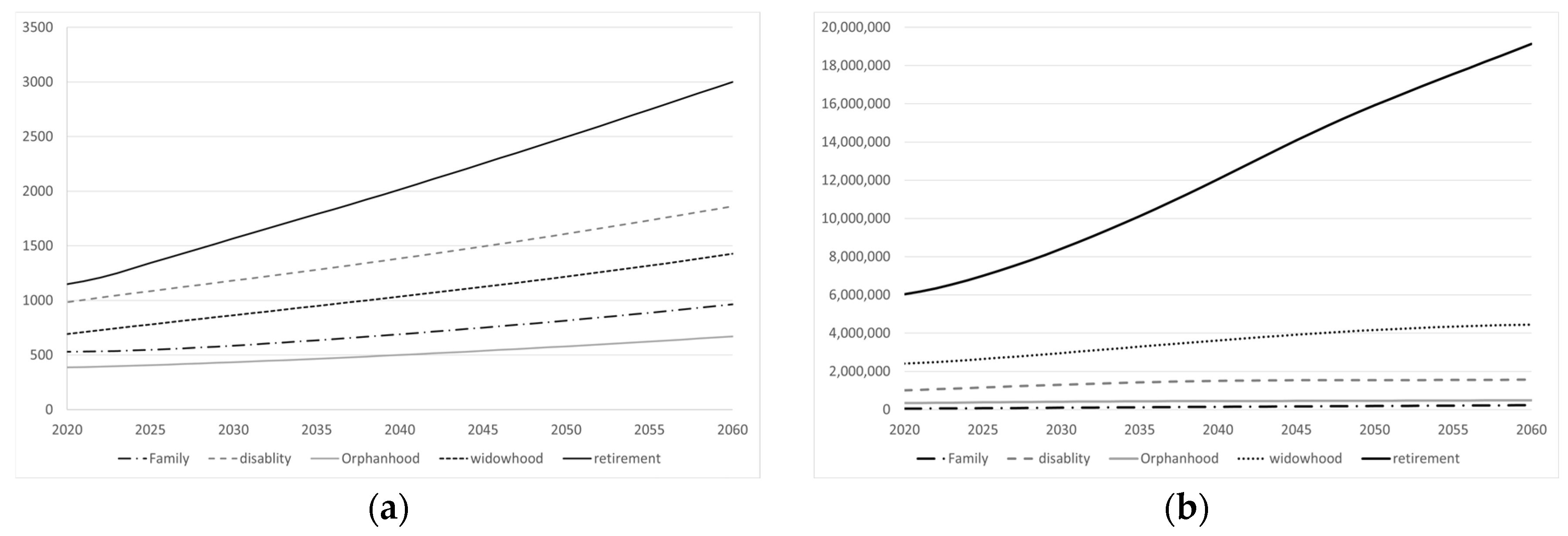
Figure 20 shows the five types of contributory pensions estimated in this microsimulation model, presenting the average pension and the number of pensioners for each of them during the projected period. The results of the previous figure are confirmed, since retirement pensions represent the greatest future expense, both due to the greater number of pensioners, in comparison to the other contributory pensions, and the average pension, which is higher.
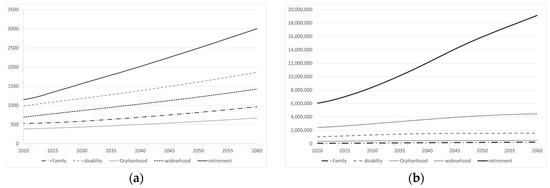
Figure 20.
(a) Average pension by type of contributory pension; (b) number of pensioners by type of contributory pension [41].
4.2. Adequacy of the Retirement Pension System
The adequacy of the pension system is a critical element when analyzing pension systems and potential reforms. A system that generates benefits to protect older individuals from poverty and ensures sufficient income is fundamental.
This paper focuses on incorporating adequacy measures with disaggregated perspective, estimating different elements that affect pension expenditure, especially retirement pensions. It begins by analyzing the evolution of pension inflows and the average initial pension over the projection period. The average retirement pension in the system is then analyzed as well as the number of retired pensioners, as shown in Figure 21.
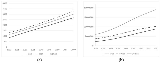
Figure 21.
(a) Average retirement pension by gender; (b) number of retirement pensions by gender [41].
The average pension demonstrates linear and consistent growth throughout the period, with annual growth rates of 2.4% per year. In terms of the total number of pensioners, we project significant growth, driven by growth rates of approximately 4.0% mid-period, tapering to 1.7% annual increases in the last decade. This trend elevates the number of pensioners from nearly 6 million to 18 million. The combination of these alongside institutional and labor market elements is propelling pension expenditures upwards.
It is possible to delve deeper into generating estimates for various levels of pension benefits— beyond the average value typically provided in most research—whether for the initial pension, existing pensions within the system, or by types of pensions and gender. As an example, Table 2 illustrates the evolution of the retirement pension for the 2nd, 4th, 6th, and 8th deciles of the income distribution in the selected years.
Table 2.
Evolution of 4 deciles of retirement pensions. Total number of pensioners [41].
The analysis of Table 2 enables the determination of whether the pension system acts as a reducer of inequality by examining the distance between the different deciles of the retirement pension distribution. As time progresses, there is an increasing dispersion in the distribution of retirement pensions. This outcome is particularly significant when conducting analyses on the adequacy of the pension system.
Continuing with a gender-disaggregated analysis, we track the evolution of initial pensions and the number of retirement inflows throughout the projected period (Figure 22).
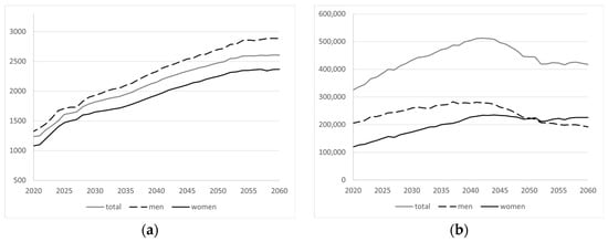
Figure 22.
(a) Initial retirement pension; (b) retirement inflows [41].
In the initial years, the growth of the initial pension is noticeably contained due to the implementation of the 2011 reform, a trend that dissipates after 2027. It is also observed that the differential between men and women is maintained over time, with amounts of EUR 2886 and EUR 2367 per month, respectively, representing 82% of the male benefit. The estimated values for the initial pension align with the range reported in the 2018 Ageing Report by the European Commission.
Regarding the inflows into the retirement system, although significantly lower for women at the beginning of the period, there is a convergence in the number of new pensioners starting from the 2050s.
The micro approach allows us to generate results with a higher level of disaggregation. For instance, Table 3 presents the initial pension for new pensioners by age in specific years.
Table 3.
Average initial pension in a 3-year projection (2020, 2030, 2040) [41].
Measuring adequacy, two concepts are commonly used: the substitution rate, which compares the average pension to the average wage in a given year, and the replacement rate (TR), measured as the first pension received by a new pensioner relative to their last wage before retirement.
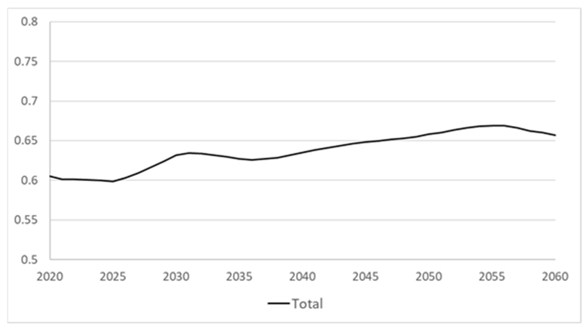
Considering the microsimulation previously described, this value can be calculated individually using the datasets. Figure 23 presents the average replacement rate for the projected period.
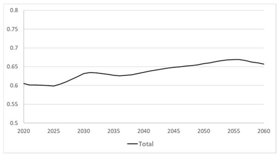
Figure 23.
Replacement rate of new retirement pensioners [41].
It is observed that, at the beginning of the period, the initial pension accounts for 60% of the last salary received for both men and women. This variable is expected to remain constant throughout the period, with a slight increase towards the end.
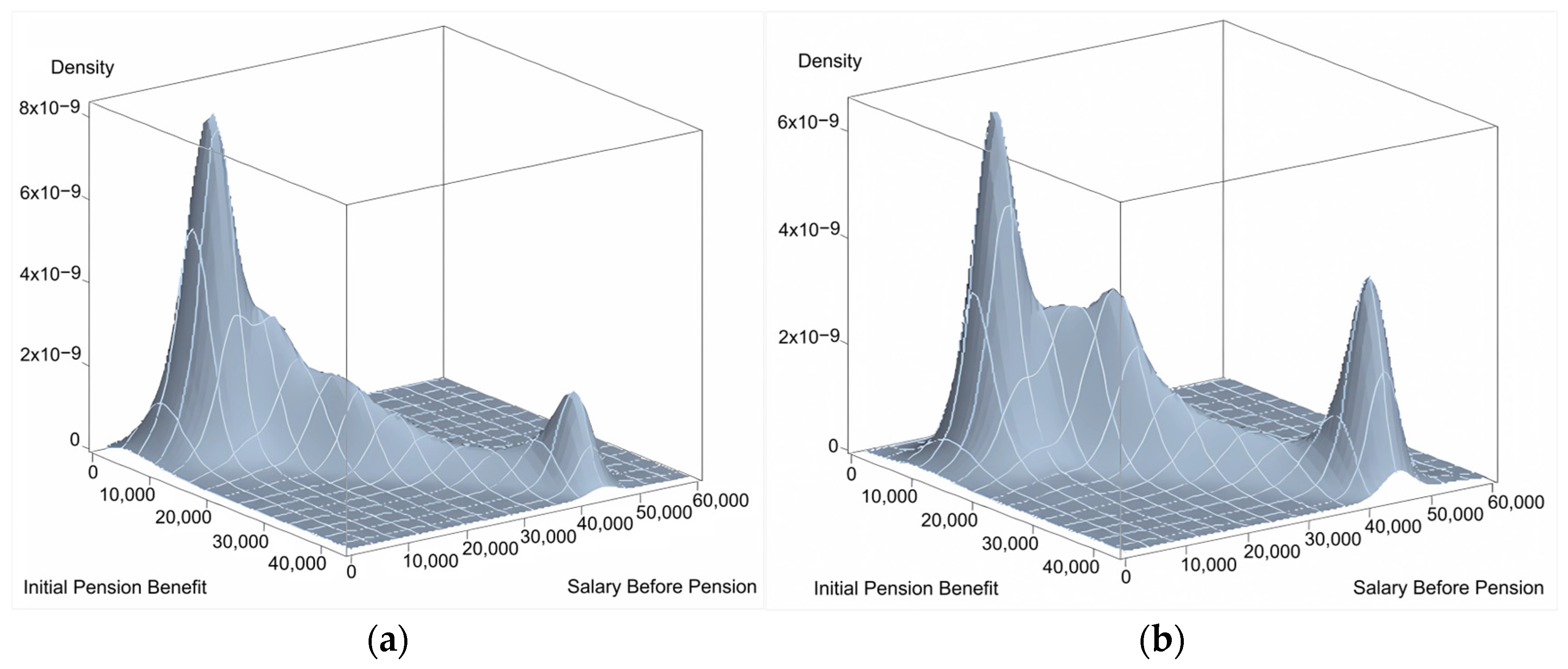
Alongside calculating the average ”replacement rate”, the micro approach allows for the generation of results with a higher level of disaggregation. For example, if one wishes to analyze the adequacy of the system for all new pensioners in a specific year, it is possible to calculate the density functions that link the two variables of interest (initial pension and last salary) using non-parametric estimations [43].
In 2025, there is a positive relationship between the initial pension and the last salary, as illustrated in the surface graph (Figure 24) through a diagonal line with a positive slope. The majority of new female pensioners receive an entry pension of EUR 10,000 per year, which is slightly higher for men. In both cases, some workers achieve the maximum pension of nearly EUR 38,000 per year, a situation that occurs more frequently among men than women.
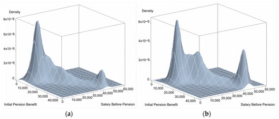
Figure 24.
(a) Initial pension and last salary of new female pensioners in 2025. Female; (b) initial pension and last salary of new female pensioners in 2025. Male [41].
These figures incorporate a key element for analyzing adequacy, as they detail the number of pensioners at each pension level. This allows for the determination of the percentage of individuals who receive a low pension, insufficient to provide adequate income in old age.
5. Conclusions
The vast majority of simulation models focus on analyzing the sustainability of pension systems using different approaches, such as accounting aggregates or general equilibrium models. The novelty of this paper lies in proposing a new simulation model for pension expenditure that not only analyses sustainability but also adequacy, offering a high degree of disaggregation in the results. To achieve this, we propose a mixed model that combines a macro approach, utilizing data from public institutions like INE and Eurostat, with a micro approach using the MCVL dataset from Spanish Social Security, which projects relevant labor market variables such as work time and wages at the individual level. This dual approach allows for the generation of gender-disaggregated calculations of various pension-related variables, introducing an innovative element of analysis previously absent in pension modeling.
In terms of sustainability, the projected pension expenditure as a proportion of GDP is expected to reach 13.9% by the end of the projection period. The inclusion of gender analysis reveals consistently lower earnings for women compared to men throughout the period, highlighting the importance of considering gender in pension systems. Regarding adequacy, disaggregated calculations of new pensions are performed and analyzed using density functions and by assessing different deciles of the pension distribution. This detailed analysis provides valuable insights into the risk of poverty among pensioners and could inform policy improvements to address income inequality and enhance pension adequacy.
Considering the characteristics of our model, there are several potential extensions that could enhance its capabilities in future research. First, replacing the current macro approach with a general equilibrium model, combined with the micro approach, could provide a more comprehensive framework for analyzing interactions between economic and demographic variables. Second, incorporating machine learning methods into the retirement decision analysis would improve the model’s predictive power and flexibility. Lastly, given the model’s emphasis on adequacy and poverty analysis, integrating the concept of ‘household’ into the databases would be highly valuable. This could be achieved by utilizing household surveys, offering richer insights into income distribution and social inequalities at a more detailed level.
Author Contributions
Conceptualization, J.V.-G., I.M.-A. and L.J.G.V.; Methodology, J.V.-G. and I.M.-A.; Software, J.V.-G.; Validation, J.V.-G. and I.M.-A.; Formal analysis, J.V.-G. and I.M.-A.; Investigation, J.V.-G., I.M.-A. and L.J.G.V.; Resources, J.V.-G. and I.M.-A.; Data curation, J.V.-G. and I.M.-A.; Writing—original draft preparation, J.V.-G. and I.M.-A.; Writing—review and editing, J.V.-G., I.M.-A. and L.J.G.V.; Visualization, J.V.-G.; Supervision, J.V.-G. and I.M.-A.; Project administration, J.V.-G. All authors have read and agreed to the published version of the manuscript.
Funding
This work was supported by funds from the Recovery, Transformation and Resilience Plan, financed by the European Union (Next Generation), through the INCIBE-UCM: “Cybersecurity for Innovation and Digital Protection” Chair. The content of this article does not reflect the official opinion of the European Union. Responsibility for the information and views expressed therein lies entirely with the authors.
Data Availability Statement
The data used in this study can be accessed through official sources such as the Spanish Statistics Office (INE), Eurostat and the Spanish Social Security.
Conflicts of Interest
The authors declare no conflicts of interest.
References
- European Commission. The 2018 Ageing Report: Economic and Budgetary Projections for the EU Member States (2016–2070); European Economy Institutional Paper No. 079; European Commission: Brussels, Belgium, 2018; Available online: http://data.europa.eu/doi/10.2765/615631 (accessed on 5 December 2024).
- Heer, B.; Polito, V.; Wickens, M.R. Population Aging, Social Security, and Fiscal Limits. J. Econ. Dyn. Control 2020, 116, 103913. [Google Scholar] [CrossRef]
- Laun, T.; Markussen, S.; Vigtel, T.C.; Wallenius, J. Health, Longevity, and Retirement Reform. J. Econ. Dyn. Control 2019, 103, 123–157. [Google Scholar] [CrossRef]
- Valls Martínez, M.d.C.; Santos-Jaén, J.M.; Amin, F.-u.; Martín-Cervantes, P.A. Pensions, Ageing and Social Security Research: Literature Review and Global Trends. Mathematics 2021, 9, 3258. [Google Scholar] [CrossRef]
- Grech, A.G. What Makes Pension Reforms Sustainable? Sustainability 2018, 10, 2891. [Google Scholar] [CrossRef]
- Godínez-Olivares, H.; Boado-Penas, M.d.C.; Pantelous, A.A. How to Finance Pensions: Optimal Strategies for Pay-as-You-Go Pension Systems. J. Forecast. 2016, 35, 13–33. [Google Scholar] [CrossRef]
- De la Fuente, A.; García, M.A.; Sánchez Martín, A.R. La Salud Financiera del Sistema Público de Pensiones Español: Proyecciones de Largo Plazo y Factores de Riesgo. Hacienda Pública Española/Rev. Public Econ. 2019, 229, 123–156. [Google Scholar] [CrossRef]
- Bazzana, D. Ageing Population and Pension System Sustainability: Reforms and Redistributive Implications. Econ. Politica 2020, 37, 971–992. [Google Scholar] [CrossRef]
- Holzmann, R.; Hinz, R. Old-Age Income Support in the 21st Century: An International Perspective on Pension Systems and Reform; The World Bank: Washington, DC, USA, 2005; Available online: https://documents1.worldbank.org/curated/en/466041468141262651/pdf/32672.pdf (accessed on 5 December 2024).
- Fisher, G.G.; Chaffee, D.; Sonnega, A. Retirement Timing: A Review and Recommendations for Future Research. Work Aging Retire. 2016, 2, 2. [Google Scholar] [CrossRef]
- Scharn, M.; Sewdas, R.; Boot, C.R.L.; Huisman, M.; Lindeboom, M.; van der Beek, A.J. Domains and Determinants of Retirement Timing: A Systematic Review of Longitudinal Studies. BMC Public Health 2018, 18, 1083. [Google Scholar] [CrossRef]
- Börsch-Supan, A.; Ludwig, A.; Winter, J. Ageing, Pension Reform and Capital Flows: A Multi-Country Simulation Model. Economica 2006, 73, 625–658. [Google Scholar] [CrossRef]
- Li, J.; O’Donoghue, C. A Survey of Dynamic Microsimulation Models: Uses, Model Structure and Methodology. Int. J. Microsimul. 2013, 6, 3–55. [Google Scholar] [CrossRef]
- Komp, K.; Johansson, S. Population Ageing in a Lifecourse Perspective: Developing a Conceptual Framework. Ageing Soc. 2016, 36, 1937–1960. [Google Scholar] [CrossRef]
- Martin, L.G. Demography and Aging. In Handbook of Aging and the Social Sciences, 7th ed.; Binstock, R.H., George, L.K., Eds.; Academic Press: San Diego, CA, USA, 2011; pp. 33–45. [Google Scholar] [CrossRef]
- De la Fuente, A.; García, M.A.; Sánchez Martín, A.R. ¿Hacia una contrarreforma de pensiones? Notas para el Pacto de Toledo. Hacienda Pública Española/Rev. Public Econ. 2020, 232, 115–143. [Google Scholar] [CrossRef]
- Jimeno, J.F. El Sistema de Pensiones Contributivas en España: Cuestiones Básicas y Perspectivas en el Medio Plazo; Documento de Trabajo No. 2000-15; Fundación de Estudios de Economía Aplicada (FEDEA): Madrid, Spain, 2000. [Google Scholar]
- Boldrin, M.; Jiménez-Martín, S.; Peracchi, F. Sistema de Pensiones y Mercado de Trabajo en España; Fundación BBVA: Bilbao, Spain, 2001. [Google Scholar]
- Alonso, J.; Herce, J.A. Balance del Sistema de Pensiones y Boom Migratorio en España. Proyecciones del Modelo Modpens de Fedea a 2050; Documento de Trabajo No. 2003-02; Fundación de Estudios de Economía Aplicada (FEDEA): Madrid, Spain, 2003. [Google Scholar]
- De La Peña, J.I.; Fernández-Ramos, M.C.; Garayeta, A.; Martín, I.D. Transforming Private Pensions: An Actuarial Model to Face Long-Term Costs. Mathematics 2022, 10, 1082. [Google Scholar] [CrossRef]
- Borella, M.; Moscarola, F.C. Microsimulation of Pension Reforms: Behavioural versus Nonbehavioural Approach. J. Pension Econ. Financ. 2010, 9, 583–607. [Google Scholar] [CrossRef]
- Van Sonsbeek, J.-M. Micro Simulations on the Effects of Ageing-Related Policy Measures. Econ. Model. 2010, 27, 968–979. [Google Scholar] [CrossRef]
- Dekkers, G.; Van den Bosch, K. Prospective Microsimulation of Pensions in European Member States. In Applications of Microsimulation Modelling; Dekkers, G., Van den Bosch, K., Eds.; Imprint Academic: Budapest, Hungary, 2016; pp. 13–33. [Google Scholar]
- Gonzalez Garibay, M. The Retirement Decision in Dynamic Microsimulation Models: An Exploratory Review. Int. J. Microsimulation 2023, 16, 19–48. [Google Scholar] [CrossRef]
- Stock, J.; Wise, D.A. The Pension Inducement to Retire: An Option Value Analysis. In Issues in the Economics of Aging; Wise, D., Ed.; University of Chicago Press: Chicago, IL, USA, 1994; pp. 205–229. [Google Scholar]
- Coile, C.; Gruber, J. Social Security and Retirement. NBER Work. Pap. Ser. 2000, 7830, 1–40. Available online: http://www.nber.org/papers/w7830.pdf (accessed on 5 December 2024).
- Baker, M.; Gruber, J.; Milligan, K. The Retirement Incentive Effects of Canada’s Income Security Programs. Can. J. Econ. 2004, 37, 261–290. [Google Scholar] [CrossRef]
- Blundell, R.; Meghir, C.; Smith, S. Pension Incentives and the Pattern of Early Retirement. Econ. J. 2002, 112, C153–C170. [Google Scholar] [CrossRef]
- Börsch-Supan, A.; Reil-Held, A.; Schunk, D. Saving Incentives, Old-Age Provision and Displacement Effects: Evidence from the Recent German Pension Reform. J. Pension Econ. Financ. 2008, 7, 295–319. [Google Scholar] [CrossRef]
- Patxot, C.; Solé, M.; Souto, G.; Spielauer, M. The Impact of the Retirement Decision and Demographics on Pension Sustainability: A Dynamic Microsimulation Analysis. Int. J. Microsimul. 2018, 11, 84–108. [Google Scholar] [CrossRef]
- Jeon, J.; Park, K. Optimal Job Switching and Retirement Decision. Appl. Math. Comput. 2023, 443, 127777. [Google Scholar] [CrossRef]
- Dybvig, P.H.; Liu, H. Lifetime Consumption and Investment: Retirement and Constrained Borrowing. J. Econ. Theory 2010, 145, 885–907. [Google Scholar] [CrossRef]
- Jeon, J.; Kwak, M.; Park, K. Horizon Effect on Optimal Retirement Decision. Quant. Financ. 2022, 23, 123–148. [Google Scholar] [CrossRef]
- Choi, K.J.; Shim, G.; Shin, Y.H. Optimal Portfolio, Consumption-Leisure and Retirement Choice Problem with CES Utility. Math. Financ. 2008, 18, 445–472. [Google Scholar] [CrossRef]
- Yang, Z.; Koo, H. Optimal Consumption and Portfolio Selection with Early Retirement Option. Math. Oper. Res. 2018, 43, 1378–1404. [Google Scholar] [CrossRef]
- Knoef, M.; Been, J.; Alessie, R.; Caminada, K.; Goudswaard, K.; Kalwij, A. Measuring Retirement Savings Adequacy: Developing a Multi-Pillar Approach in the Netherlands. J. Pension Econ. Financ. 2016, 15, 55–89. [Google Scholar] [CrossRef]
- Chia, N.C.; Tsui, A.K.C. Life Annuities of Compulsory Savings and Income Adequacy of the Elderly in Singapore. J. Pension Econ. Financ. 2003, 2, 41–65. [Google Scholar] [CrossRef]
- Buddelmeyer, H.; Freebairn, J.; Kalb, G. Evaluation of Policy Options to Encourage Welfare to Work. Aust. Econ. Rev. 2006, 39, 273–292. [Google Scholar] [CrossRef]
- Stensnes, K.; Stølen, N.M. Pension Reform in Norway: Microsimulating Effects on Government Expenditures, Labour Supply Incentives, and Benefit Distribution; Discussion Papers No. 524; Statistics Norway, Research Department: Oslo, Norway, 2007; Available online: https://hdl.handle.net/10419/192506 (accessed on 5 December 2024).
- Eurostat. Europop2019—Population Projections at National Level (2019–2100). Available online: https://ec.europa.eu/eurostat/web/population-demography/population-projections/database (accessed on 5 December 2024).
- Spanish Social Security. Continuous Sample of Working Lives (MCVL). Available online: https://www.seg-social.es/wps/portal/wss/internet/EstadisticasPresupuestosEstudios/Estadisticas/EST211 (accessed on 5 December 2024).
- Spanish Statistics Office (Instituto Nacional de Estadística, INE). Mortality Tables by Year, Sex, Age, and Functions. Available online: https://www.ine.es/jaxiT3/Tabla.htm?t=27153&L=0 (accessed on 5 December 2024).
- Härdle, W.; Werwatz, A.; Müller, M.; Sperlich, S. Nonparametric and Semiparametric Models; Springer Series in Statistics; Springer: Berlin/Heidelberg, Germany, 2004. [Google Scholar] [CrossRef]


Disclaimer/Publisher’s Note: The statements, opinions and data contained in all publications are solely those of the individual author(s) and contributor(s) and not of MDPI and/or the editor(s). MDPI and/or the editor(s) disclaim responsibility for any injury to people or property resulting from any ideas, methods, instructions or products referred to in the content. |
© 2025 by the authors. Licensee MDPI, Basel, Switzerland. This article is an open access article distributed under the terms and conditions of the Creative Commons Attribution (CC BY) license (https://creativecommons.org/licenses/by/4.0/).