Article

A Two-Stage Adaptive Differential Evolution Algorithm with Accompanying Populations

1
School of Science, Southwest Petroleum University, Xindu Road, Chengdu 610500, China
2
Institute for Artificial Intelligence, Southwest Petroleum University, Xindu Road, Chengdu 610500, China
3
National Key Laboratory of Oil and Gas Reservoir Geology and Exploitation, Southwest Petroleum University, Xindu Road, Chengdu 610500, China
4
School of Energy, Geoscience, Infrastructure and Society, Heriot-Watt University, Riccarton Mains Road, Edinburgh EH14 4AS, Scotland, UK
*
Author to whom correspondence should be addressed.
Mathematics 2025, 13(3), 440; https://doi.org/10.3390/math13030440
Submission received: 31 December 2024 / Revised: 19 January 2025 / Accepted: 25 January 2025 / Published: 28 January 2025
(This article belongs to the Section E: Applied Mathematics)

Abstract

:
Stochastic simulations are often used to determine the crossover rates and step size of evolutionary algorithms to avoid the tuning process, but they cannot fully utilize information from the evolutionary process. A two-stage adaptive differential evolution algorithm (APDE) is proposed in this article based on an accompanying population, and it has unique mutation strategies and adaptive parameters that conform to the search characteristics. The global exploration capability can be enhanced by the accompanying population to achieve a balance between global exploration and local search. This algorithm has proven to be convergent with a probability of 1 using the theory of Markov chains. In numerical experiments, the APDE is statistically compared with nine comparison algorithms using the CEC2005 and CEC2017 standard set of test functions, and the results show that the APDE is statistically superior to the comparison methods.

1. Introduction

Among many evolutionary optimization methods, differential evolution (DE) is a heuristic stochastic search algorithm based on population differences. For its simple structure, easy implementation, fast convergence, and robustness, DE is widely used in various fields such as data mining [1], pattern recognition [2], digital filter design [3], artificial neural networks [4], and electromagnetism [5]. However, the performance of DE depends seriously on the control parameters and mutation strategies. Inappropriate parameters or mutation strategies will reduce the convergence performance of the algorithm or fall into the local optimum. Therefore, many scholars have conducted research on the update strategy and algorithmic structure of DE algorithms in recent years. Current improvements in DE can mainly be categorized as follows: multi-population [6], multi-evolutionary model [7], parameter adaptive [8,9], strategy and search space adaptive [10,11,12,13], variant strategy updating [14,15,16,17], online algorithmic configurations [18], parameter free [19], etc.
Incorporating multi-population or multi-evolution modules into the algorithm can improve the global search capability and convergence rate of the evolutionary algorithm. For example, DSPPDE [6] employs the idea of isolated evolution and information exchanging in parallel DE algorithms via serial program structure; MEDE [7] realizes multi-strategy cooperation based on the fact that each evolution strategy of DE has common peculiarities but different characteristics; MCDE [8] uses a population structure with multi-populations so that covariance learning can establish a proper rotational coordinate system for the crossover operation, and it uses adaptive control parameters to balance the ability of population surveys and convergence; BMEA-DE [9] divides the population into three sub-populations based on fitness, which uses separate variation strategies and control parameters for different populations.
On the other hand, the parameters are critical to the accuracy of DE and its convergence rate. For example, if the mutation rate of CR is too small, it will reduce the ability of the algorithm in the global search and eventually fall into the local optimum; if the mutation rate of CR is too large, it is computationally consuming, resulting in a decrease in the speed of convergence of the algorithm. Therefore, many scholars have introduced adaptive operators to adjust parameters based on certain information. For example, ADE [10] introduces an adaptive mutation operator according to the comparison between each individual’s fitness and the best one’s fitness, and it adds a competition operation with a random new population to improve the global search capability. ISADE [11] incorporates space-adaptive ideas into DE to realize the automatic search for the suitable space and improve the convergence rate and accuracy. IDE [12] generates the initial population with a reverse learning strategy and selects individuals via the Metropolis criterion of simulated annealing algorithms. APSDE [13] optimizes the mutation strategy and control parameters through the accompanying population, in which individuals are composed of suboptimal solutions.
The mutation operator of DE has high randomness and is mainly composed of only one evolutionary direction. This kind of operator makes DE prone to problems such as premature phenomena and slow convergence speeds. Moreover, DE cannot realize both a global search of space and local optimization operations at the same time. As a result, many scholars have conducted many studies on the update strategy of DE. SSDE [14] employs an opposition-based learning method to enhance global convergence performance when producing the initial population. GSDE [15] optimizes the exploitation ability with Gaussian random walk and local search performances with simplified crossovers and mutations based on individuals’ performance. SEFDE [16] achieves the feedback adjustment of mutation strategies via the stage of the individual, which can be self-adaptively determined by designing the state judgment factor. Consequently, the algorithm can obtain a trade-off between exploration and exploitation. HHSDE [17] introduces a new mutation operation to improve the efficiency of mutations within the new harmony generation mechanics of the harmony algorithm (HS).
In addition, some algorithmic configuration methods have been developed in recent years. For example, OAC [18] selects a trial strategy for vector generation via the multi-armed bandit algorithm, in which kernel density estimation is employed to tune the control parameters during the searching process.
In summary, most of the studies on the improvements in DE are focused on the strategies of mutation operators and control parameters, often disregarding the algorithm’s distinctive search characteristics across various stages.
In general, evolutionary algorithms are generally divided into two stages. The main task of the first stage of the algorithm is to explore the target region globally. Meanwhile, in the second stage, the focus shifts to narrowing down the search region to the neighborhood of the better-performing particles, aiming at finding the locally optimal solutions in the region and avoiding premature convergence. Thus, in this paper, a novel two-stage algorithm is proposed. This algorithm has two kinds of populations and constructs new mutation patterns with adaptive direction vector weight factors and crossover factors. As a result, it is able to achieve fast convergence and avoid the local optimum.

2. A Two-Stage Adaptive Differential Evolution Algorithm (APDE) with Accompanying Populations

In this section, a two-stage adaptive differential evolutionary algorithm with accompanying populations is proposed. In this algorithm, we use different mutation strategies for the test and accompanying populations in order to maximize the mutation efficiency.
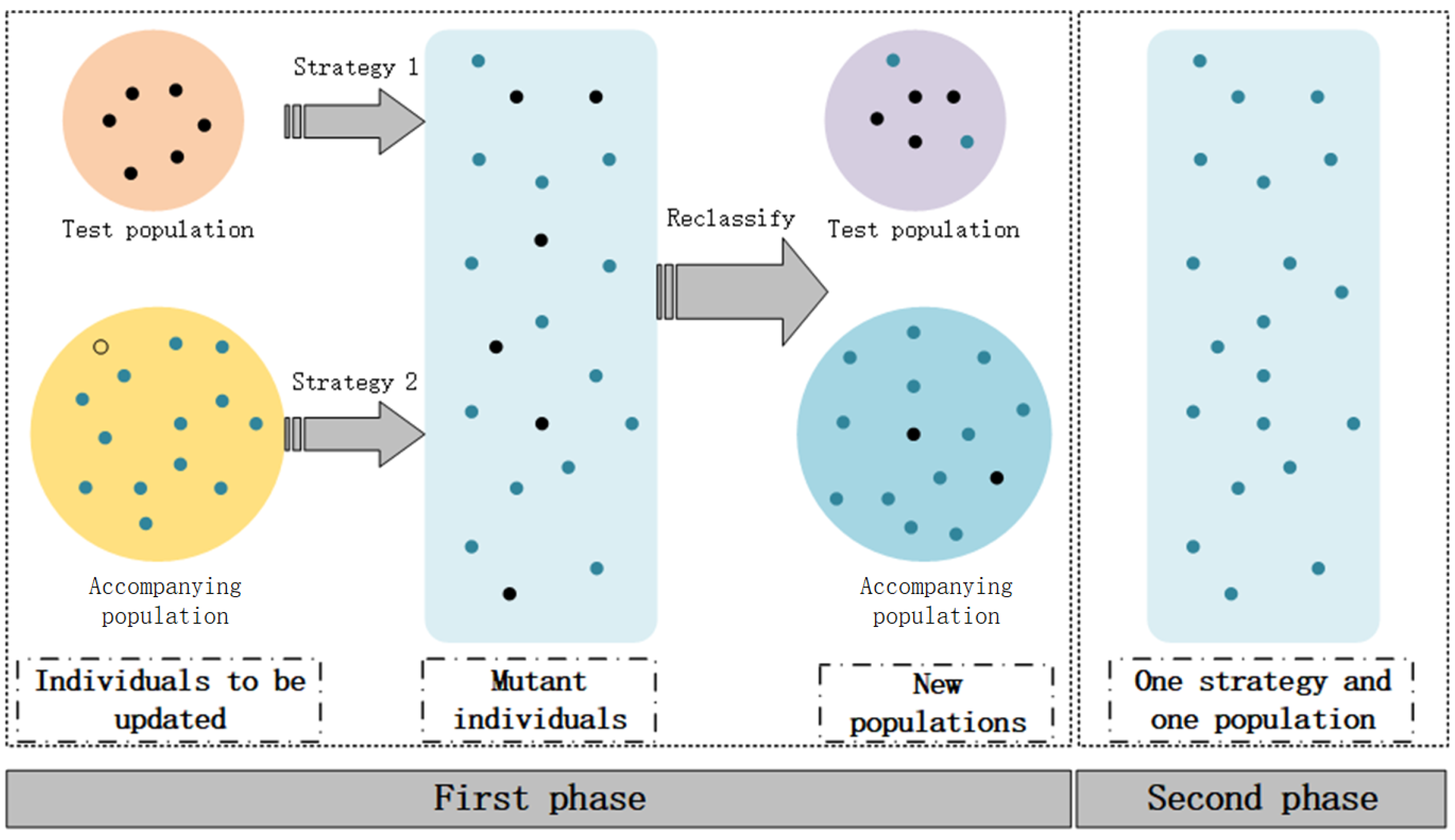
The updated individuals will be reclassified according to their fitness value, which ensures evolutionary diversity and achieves information exchange between populations. In addition, APDE divides the algorithm into two stages according to the search characteristics of the evolutionary algorithm. Therefore, the algorithm can quickly converge in the early stage and escapes local optimum efficiently in the later stage by enhancing its stochastic mutability. This operation can help improve computing efficiency and maintain convergence speeds. Figure 1 depicts the specific operation of each stage in APDE.

2.1. Initialization

APDE uses the Good Point Set Method [20] to generate the initial population. Then, the initial individuals are evenly distributed in the search space to overcome blindness and randomness and improve population diversity. The initialization formulas are as follows:
r j = 2 cos 2 π × j 2 π × j 2 D + 3 2 D + 3 ,
x i j 0 = x i j L + mod r j × i , 1 × x i j U x i j L .
Here, j 1 , 2 , , D , i 1 , 2 , , N . x i j L and x i j U are the upper and lower bounds of the range of values taken by the jth component x i j of the individual.

2.2. Population Segmentation

The population of APDE is divided into 2 classes. One is the test population, for which its main function is to explore the optimal solution based on the information of the optimal individuals. The other one is the accompanying population, which has lower fitness values and is randomly distributed throughout the entire search space. Its primary function is to explore uncharted regions and augment population diversity. After multiple trials, APDE uses a empirical 3:7 ratio to divide the population, and the individuals are reordered according to the fitness value at the end of each iteration. The segmentation operation can be specifically expressed as follows:
f I = s o r t f x 1 f x 2 f x N P ,
c i = 0 , i f f x i g f 0.3 N P , 1 , o t h e r w i s e .
where c i is the population classification information for the ith individual. Here, 0 indicates the test population, and 1 indicates the accompanying population.

2.3. Improved Mutation Operator

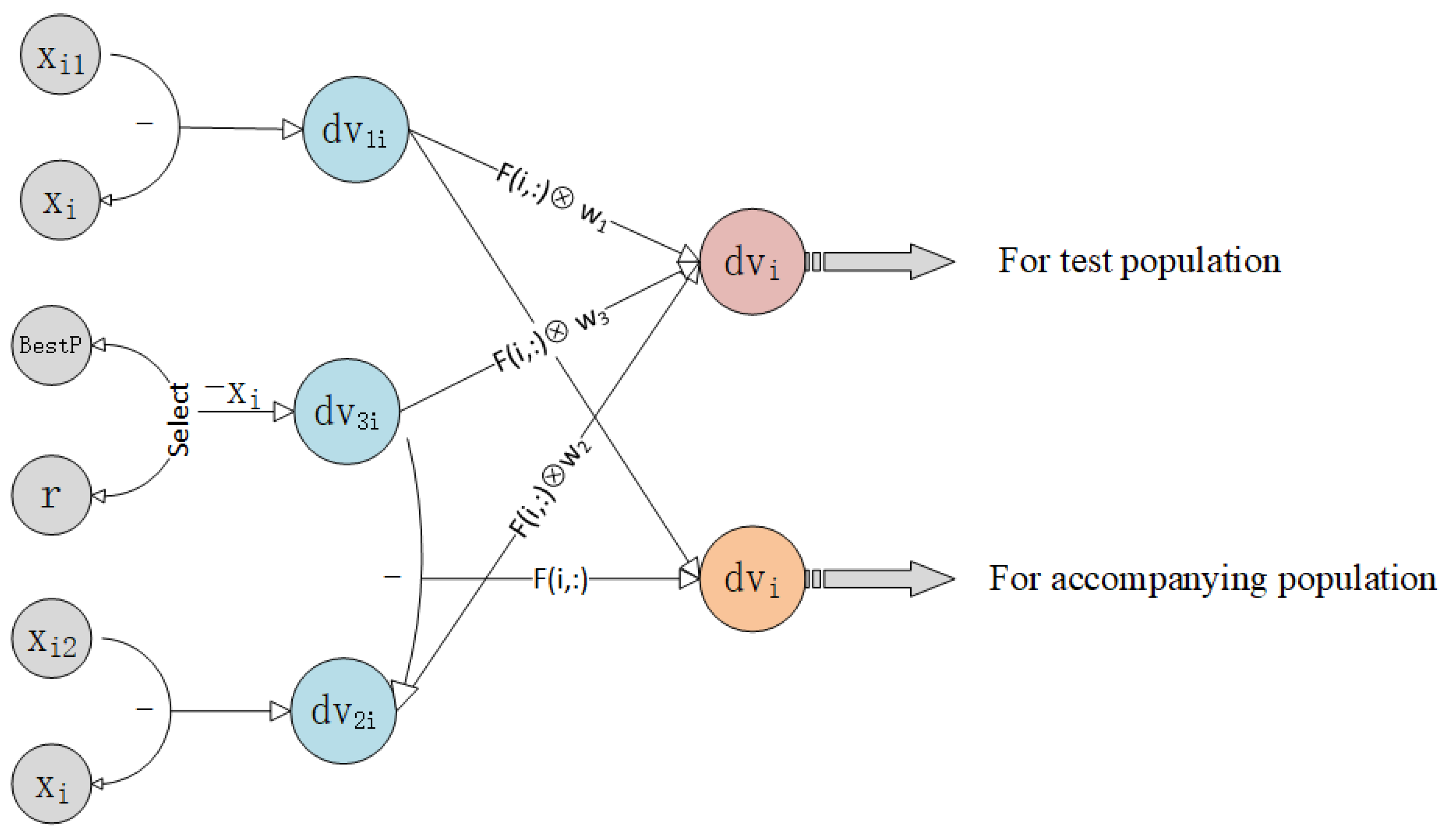
In 2022, Civicioglu [19] proposed an elitist mutation operator in the Bernstein–Levy differential evolution(BDE) algorithm, which uses three vectors to generate mutation directions. The generation process of this mutation operator is partially elitist. This structure enhances the algorithm’s local search capability and improves the algorithm’s ability to generate effective mutation patterns. The first two direction vectors d v 1 and d v 2 are generated by obtaining the difference in the two different individuals selected at random. The generation method is as follows:
d v 1 = x i 1 x i = 1 : N i 1 = p e r m u t e 1 : N , d v 2 = x i 2 x i = 1 : N i 2 = p e r m u t e 1 : N , i 1 i 2 , a n d i 1 , i 2 1 : N .
where p e r m u t e 1 : N denotes the vector replacement function.
d v 3 is generated via the location information about the current optimal solution. The information can be used directly or after numerical perturbation within the limits of the relevant search space.
(1) When current optimal solution B e s t P is used directly,
d v 3 i = B e s t P x i .
(2) When current optimal solution B e s t P is used after applying a numerical perturbing progress,
r 0 = B e s t P + k 1 3 x i U B e s t P ,
r = r + k 2 3 x i L r 0 ,
d v 3 i = r x i .
k 1 and k 2 are random numbers obeying a uniform distribution in 0 , 1 .
BDE selects these two generation methods with a probability of 50%. However, this strategy is too dependent on randomness and does not match the search characteristics of the algorithm. As a result, it slows down the convergence of the algorithm in the early stage and squanders computational resources. Obviously, the generation in (1) is more conducive for the algorithm for quickly approaching the current optimal solution, while the generation in (2) is more suitable for enhancing the global search capability of the algorithm. Therefore, the algorithm in this paper innovates the mutation strategy as follows.
d v 3 i = B e s t P x i , i f c i = 1 , r x i , o t h e r w i s e .
To synthesize the three direction vectors in the test population, an adaptive weight factor is proposed in this paper according to the iterative process of the algorithm:
w 1 = w 2 = r a n d N , 1 ,
w 3 = w 1 + o n e s N , 1 w 1 × 0.6 × sin π 2 × 1 e p k e p o c h .
where w 1 , w 2 , and w 3 are the combined weight factors of d v 1 , d v 2 , and d v 3 ; e p k is the current iteration number; e p o c h is the maximum number of iterations. It is easy to know from the above equations that d v 1 and d v 2 are generated in the same way, so they have the same weights. In order to fully utilize the leadership of the current optimal solution, the weight of d v 3 should be higher than w 1 and w 2 and increase with the number of iterations. As a result, d v 3 is a direction vector with elite strategies.
For the accompanying population, its combined direction vector consists of the difference between direction vectors d v 2 and d v 3 . This structure enables the accompanying population to have a stronger exploration ability.
In summary, the combined direction vector d v is defined as follows:
d v i , : = F i , : w 1 d v 1 i , : + w 2 d v 2 i , : + w 3 d v 3 i , : , i f c i = 0 , d v 1 i , : + F i , : d v 3 i , : d v 2 i , : , o t h e r w i s e .
where ⊗ denotes the Hadamard product. F ( i , : ) is the value of the evolutionary step size of the ith individual. The step size is generated by the Levy distribution, which has more powerful exploratory capabilities. Figure 2 exemplifies the specific way in which the mutation operates.

2.4. Crossover and Selection

The crossover rate plays a critical role in the global searching ability and convergence speed of DE, which are conflicting. Thus, the key is to find a suitable crossover rate to balance the convergence rate and the global searching ability. The adaptive exponential distribution is employed to generate crossover rates rather than the traditional constant value in APDEs, which enables the algorithm to efficiently escape the local optimum in later stages.
C R = 0.3 + 0.6 × 1 e 5 e p k e p o c h .
The crossover process is controlled by the mapping matrix from BDE, in which the permutation operation is employed to embed the crossover rate CR into the searching directions of each individual. This embedding map is initialized as an N × D zero matrix. At each BDE iteration step, the numerical values of the map elements are updated via the following Equation (15):
m a p i , h 1 : [ C R × D ] = 1 ,
x ˜ = x + m a p d v .
where h = p e r m u t e d ( 1 : D ) , and  x ˜ is an offspring generation after crossover and mutation. When the value of x ˜ is outside the search region, it will be adapted by a random number within the search region.
Finally, we can update the populations as follows.
x i g + 1 = x ˜ i g , i f f x ˜ i < f x i , x i g , o t h e r w i s e .

2.5. Two-Stage Evolutionary Strategy

As is known to all, it is challenging for evolutionary algorithms to avoid falling into a local optimum without reducing the algorithm’s convergence rate. Indeed, it is to balance the randomness and optimization of the search within the algorithmic process. Thus, we focus on solving the problem with different search goals in the early and later stages of the algorithm.
A multi-population strategy can enhance the algorithm’s search ability and population diversity, enabling rapid convergence in the early stages and emphasizing selecting random mutation strategies in the later stage.
In the two stages of the proposed algorithm, we use half of the maximum iteration as the dividing point, and we implement different mutation operator selection strategies. In the first stage, APDE formulates different mutation strategies with various populations, thus achieving effective information exchange between populations. In the second stage, the quality of individuals in the test and accompanying populations increases, and the efficiency of multi-population strategy decreases. As a result, the test and accompanying populations are merged in this stage, and the mutation strategies are selected with equal probability. This operation increases the algorithmic randomness to enhance the search capability of the algorithm in the later stages. The pseudo-code of the APDE is as shown in Algorithm 1.
Algorithm 1 APDE Algorithm.
1:
/ / Initialization;
2:
r j = 2 c o s ( ( 2 π j ) / ( 2 D + 3 ) ) ;
3:
x i j ( 0 ) = x i j L + m o d ( i r j , 1 ) × ( x i j U x i j L ) ;
4:
B e s t X = m i n f ( x i ) | i 1:NP;
5:
for  I t e r a t i o n = 1 t o M a x C y c l e  do
6:
     / / Population Segmentation;
7:
     [ f I ] = s o r t ( [ f ( x 1 ) f ( x 2 ) f ( x N P ) ] ) ;
8:
    if  f ( x i ( g ) ) f 0.3 N P  then
9:
         c i = 0
10:
    else
11:
         c i = 1
12:
    end if
13:
     / / Generation of Random Direction Vectors;
14:
     d v 1 = x i 1 x i = 1 : N P | i 1 = p e r m u t e ( [ i : N ] )
15:
     d v 2 = x i 2 x i = 1 : N P | i 2 = p e r m u t e ( [ i : N ] ) | i 1 i 2 , a n d i 1 , i 2 [ 1 : N ] ;
16:
     / / Generation of Evolutionary Step Size Value;
17:
    for  i = 1 to N P  do
18:
         F ( i , 1 ) = 1 / ( β · ϕ ) | ϕ Γ ( α = 0.50 , β / 2 | U 1 : 16 );
19:
         F ( 1 : N P , 1 : D ) = ( ( F ( 1 : N P , 1 ) ) T ) ( 1 : N P , 1 ) · O ( 1 , 1 : D )
20:
    end for
21:
     / / First Phase;
22:
    if  I t e r a t i o n 1 / 2 M a x C y c l e  then
23:
        if  c i = 0  then
24:
            d v 3 i = B e s t X x i ;
25:
            d v ( i , : ) = F ( i , : ) ( w 1 d v 1 ( i , : ) + w 2 d v 2 ( i , : ) + w 3 d v 3 ( i , : ) ) ;
26:
        else
27:
            d v 3 i = r x i ;
28:
            d v ( i , : ) = d v 1 ( 1 , : ) + F ( i , : ) ( d v 3 ( i , : ) d v 2 ( i , : ) ) ;
29:
        end if
30:
    end if
31:
     / / Second Phase;
32:
    if  I t e r a t i o n > 1 / 2 M a x C y c l e  then
33:
        if  a < b | ( a , b ) U ( 0 , 1 )  then
34:
            d v 3 i = B e s t X x i ;
35:
        else
36:
            d v 3 i = r x i ;
37:
        end if
38:
        if  a < b | ( a , b ) U ( 0 , 1 )  then
39:
            d v ( i , : ) = F ( i , : ) ( w 1 d v 1 ( i , : ) + w 2 d v 2 ( i , : ) + w 3 d v 3 ( i , : ) ) ;
40:
        else
41:
            d v ( i , : ) = d v 1 ( 1 , : ) + F ( i , : ) ( d v 3 ( i , : ) d v 2 ( i , : ) ) ;
42:
        end if
43:
    end if
44:
     / / Crossing and Selection;
45:
     m a p ( i = 1 : N , j = 1 : D ) = 0 ;
46:
     C R = 0.3 + 0.6 × ( 1 e 5 e p k e p o c h ) ;
47:
    for  i = 1 to N P  do
48:
         m a p ( i , h ( 1 : [ C R × D ] ) ) = 1 ;
49:
    end for
50:
     / / Generation of Trial Pattern Vectors;
51:
     x ˜ = x + m a p d v ;
52:
     / / Boundary Control Mechanism;
53:
    for  i = 1 to N P  do
54:
        for  j = 1 to D do
55:
           if  x ˜ i j < l o w j o r x ˜ i j > u p j  then
56:
                x ˜ i j = l o w j + δ · ( u p j l o w j ) | δ U ( 0 , 1 ) ;
57:
           end if
58:
        end for
59:
    end for
60:
     / / Update;
61:
    for  i = 1 to N P  do
62:
        if  f ( x ˜ i ) < f ( x i )  then
63:
            [ x i , f ( x i ) ] = [ x ˜ i , f ( x ˜ i ) ] ;
64:
        end if
65:
    end for
66:
     f ( x γ ) = m i n f ( x i ) | i 1 : N P ;
67:
     [ B e s t X , B e s t O b j v a l ] = [ f ( x γ ) , x γ ] .
68:
end for

3. Convergence Analysis of APDE

In this section, the convergence of APDE is analyzed using the tool of Markov chains [21]. It is shown that the presented algorithm converges to the global optimum in probability.
Definition 1. 
Let a random sequence X n ; n 0 consist of random variables taking values on a discrete set; the totality of the discrete values is denoted as H L = j . H L is called the state space. If for n 1 , i k H L k n + 1 , there is
P X n + 1 = i n + 1 X n = i n , , X 0 = i 0 = P X n + 1 = i n + 1 X n = i n .
Then, X n ; n 0 is called a Markov Chain [21].
The state space H L of the random sequence X n ; n 0 can either be finite or infinite states as needed, and for the differential evolution class of algorithms, we consider H L to be finite.
Definition 2. 
Let m and n be positive integers. If the Markov Chain is in state i at time m, the probability of transferring to state j after n steps is P i j m , m + n = P X m + n = j X m = i . If the corresponding transfer probabilities are independent of time m, that is, P i j m , m + n = P i j n , the Markov chain X n ; n 0 is said to be time-homogeneous [21].
Lemma 1. 
When the crossover rate C R is fixed, the population sequence X n ; n 0 of APDE is a finite time-homogeneous Markov Chain.
Proof. 
Let the length of individuals be M, the population size be N, and the dimension of the state space be v; then, the size of the state space is v N M . As the individuals in APDE take real values and the state space of the population sequence is a finite set under finite precision conditions, the sequence of populations is finite. Also, the mutation, crossover, and selection operators of the population sequence in APDE are independent with time t when the crossover rate is a constant. The next state X t + 1 is solely dependent on the current state X t . Therefore, the sequence of populations is time-homogeneous. As a result, X n ; n 0 is a finite time-homogenous Markov Chain. □
Let X t = x 1 ( t ) , x 2 ( t ) , , x N ( t ) be a population sequence during the tth iteration. x i ( t ) is an individual in X t , and f is the fitness function on X t . Let
f * = m i n f ( x ) , x X t
be the global optimal fitness value; then, we have the following definition.
Definition 3. 
Let f t = m i n f ( x i ( t ) ) , i = 1 , 2 , , N be a sequence of random variables. The variables in the sequence denote the best fitness of the population in the state at time t. An algorithm is said to be convergent if and only if
lim t P f t = f * = 1 .
This definition indicates that algorithm convergence means that the probability of containing the global optimal solution in the population is almost 1, as the algorithm iterates through a sufficient number of generations.
Theorem 1. 
When the number of iterations of the algorithm is large enough, the APDE algorithm converges to the optima of the problem with a probability of 1.
Proof. 
Let p i ( t ) be the probability that population X t is in state s i , p i j ( t ) be the probability that population X t moves from state s i to state s j , S be the state collection, I be a set consisting of optimal states, and C R be a constant value. Note that p t = i I p i ( t ) ; by the nature of Markov chains, we have
p t + 1 = s i S j I p i ( t ) p i j ( t ) = i I j I p i ( t ) p i j ( t ) + i I j I p i ( t ) p i j ( t ) .
Moreover,
i I j I p i ( t ) p i j ( t ) + i I j I p i ( t ) p i j ( t ) = i I p i ( t ) = p t .
It is equal to
i I j I p i ( t ) p i j ( t ) = p t i I j I p i ( t ) p i j ( t ) .
So, there is
0 p t + 1 = i I j I p i ( t ) p i j ( t ) + p t i I j I p i ( t ) p i j ( t ) i I j I p i ( t ) p i j ( t ) + p t .
After crossover and mutation, an individual will not be selected when its fitness value is worse than the current optimal solution, and there is
i I j I p i ( t ) p i j ( t ) = 0 .
Then,
0 p t + 1 p t .
So,
lim t p t = 0 .
This is because
lim t P f t = f * = 1 i I p i ( t ) = 1 lim t p t = 1 .
We have
lim t P f t = f * = 1 .
In APDE, C R is adaptive in the range of ( 0.3 , 0.9 ) . The probability p i j ( t ) is determined primarily by the probability of state transfers resulting from the mutation process. It is calculated as follows:
p ( v , s i ) s j ( t ) = n = 1 N K ( n ) ,
K ( n ) = ( 1 C R ) × S e l ( m a p ( i , n ) = 0 ) + C R × S e l ( m a p ( i , n ) = 1 ) ,
S e l ( x ) = 1 , x i s t r u e , 0 , x i s f a l s e .
Here, m a p ( i , n ) denotes the mutation locus generated for the nth dimension of the ith individual. N denotes the dimension of the optimization problem.
From the previous proof, we can conclude that the probability of the optimal solution being included in the global optimum converges to 1 when K ( n ) takes a lower bound of 0.1 or an upper bound of 0.9. Additionally, we have
lim t P i j ( t | K ( n ) = 0.1 ) lim t P i j ( t | C R ( 0.3 , 0.9 ) ) lim t P i j ( t | K ( n ) = 0.9 ) .
It can be shown that when C R is taken adaptively in ( 0.3 , 0.9 ) , the conclusion can still be reached using the Squeeze Theorem [22].
In summary, APDE can find the optimal solution with a probability of 1 under the condition that the number of iterations is sufficiently large.

4. Numerical Experiment

In this paper, we employ the test functions in CEC2005 and CEC2017 to verify the performance of APDE, the specific information of which is listed in Appendix A and Appendix B. The algorithm of this paper is compared to six DE-type variants and three other types of intelligent optimization algorithms. Each algorithm is set to run 30 times independently, with the maximum number of function evaluations set at 1000 × D . The values of the dimension D are given in Table A1 and Table A2 in Appendix A. Finally, we used the Wilcoxon signed-rank test to assess the significant difference between APDE and the competition algorithms.

4.1. Comparative Analysis with APDE and DE-Type Algorithms

In this section, CoDE [23], DE [24], BDE, JADE [25], NSDE [26], and SaDE [27] are selected as comparisons to verify the performance of APDE. In Table 1, the initial values of their internal parameters are listed, and the experimental results are shown in Table 2 and Table 3. The results show that APDE achieves optimal values with respect to 16 test functions in CEC2005 and 13 test functions in CEC2017. Although APDE fails to achieve the best results in the remaining test functions, it still performs well in several comparative algorithms. Among the 16 multi-peak test functions of CEC2005, APDE fails to find the optimal solution in only three test functions. This indicates that APDE has a strong ability to jump out of the local optimum and still maintains good optimization performance with respect to multi-extreme problems.
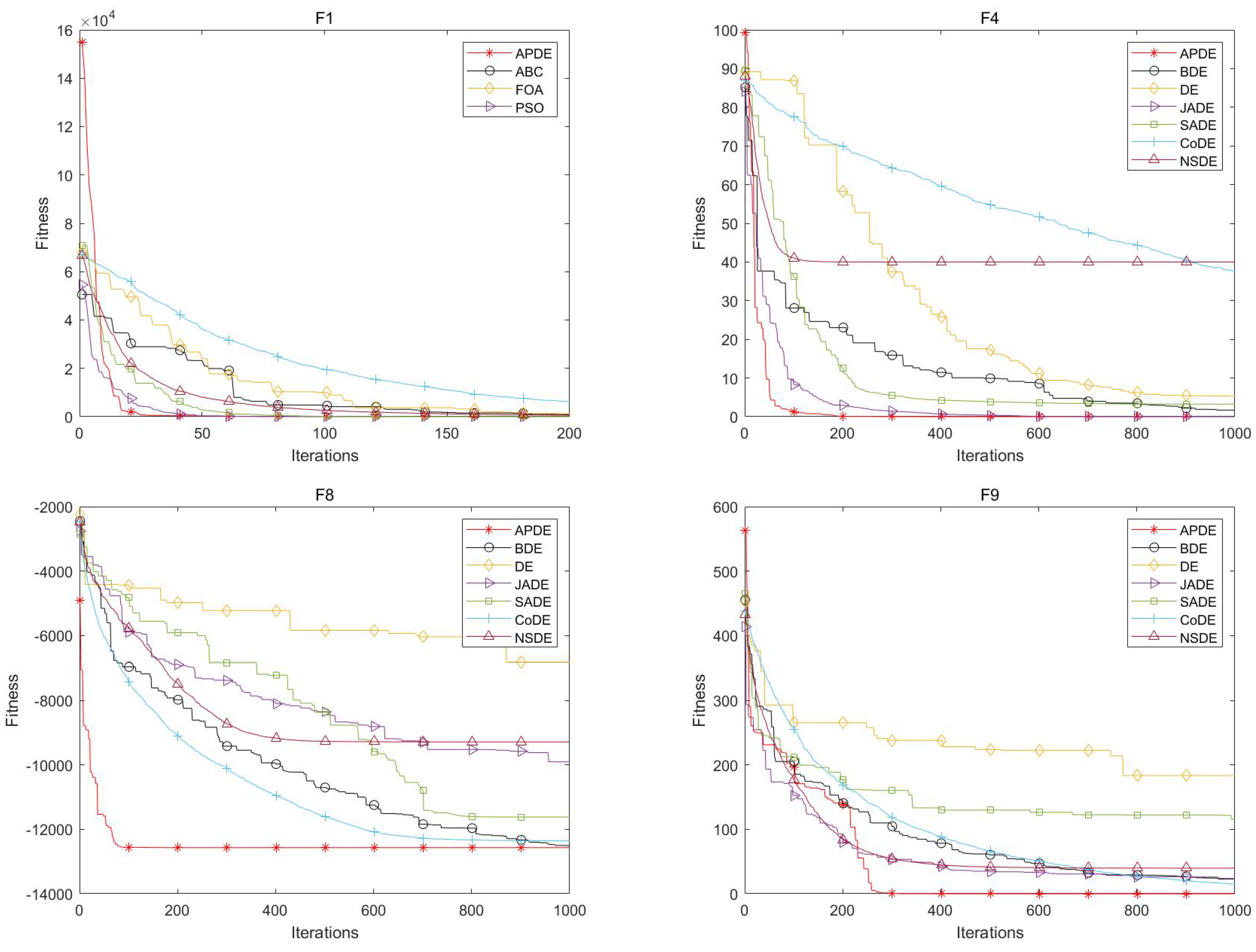
The convergence curves of the six comparison algorithms with respect to test functions F1, F4, F8, and F9 in CEC2005 are illustrated in Figure 3. The horizontal coordinate is the number of iterations, and the vertical coordinate is the adaptation value. From these figures, it can be seen that the convergence curve of APDE is significantly faster than that of the comparison algorithms, especially with respect to F8. For problem F8, APDE is able to converge to the optimal solution more quickly, while the other comparative algorithms all appear to fall into the phenomenon of the local optimum, resulting in slow convergence or being unable to converge to the optimal solution.
Figure 4 shows the convergence curves of the six comparison algorithms on test functions F5, F8, F20, and F26 in CEC2017. It can be seen that the convergence curve of APDE is faster than the comparison algorithms and has an extremely strong global search capability. Taking F20 as an example, we find that APDE appears to fall into the local optimum at about 100 iterations, and the convergence speed slows down significantly but soon jumps out of the local optimum and rapidly approaches the optimal solution. In contrast, other algorithms converge much slower after falling into a local optimum and fail to jump out of that search region.

4.2. Comparative Analysis with APDE and Non-DE Algorithms

In this section, three algorithms, FOA [28], PSO [29], and ABC [30], are selected for comparison to verify the performance of APDE. The initial values of the internal parameters of the comparison method are given in Table 4. The experimental results in Table 5 and Table 6 show that APDE achieved optimal values for 17 test functions in CEC2005 and 27 test functions in CEC2017. Although APDE failed to achieve the best results on the remaining eight functions, it still ranked second or found the optimal value among several comparative algorithms.
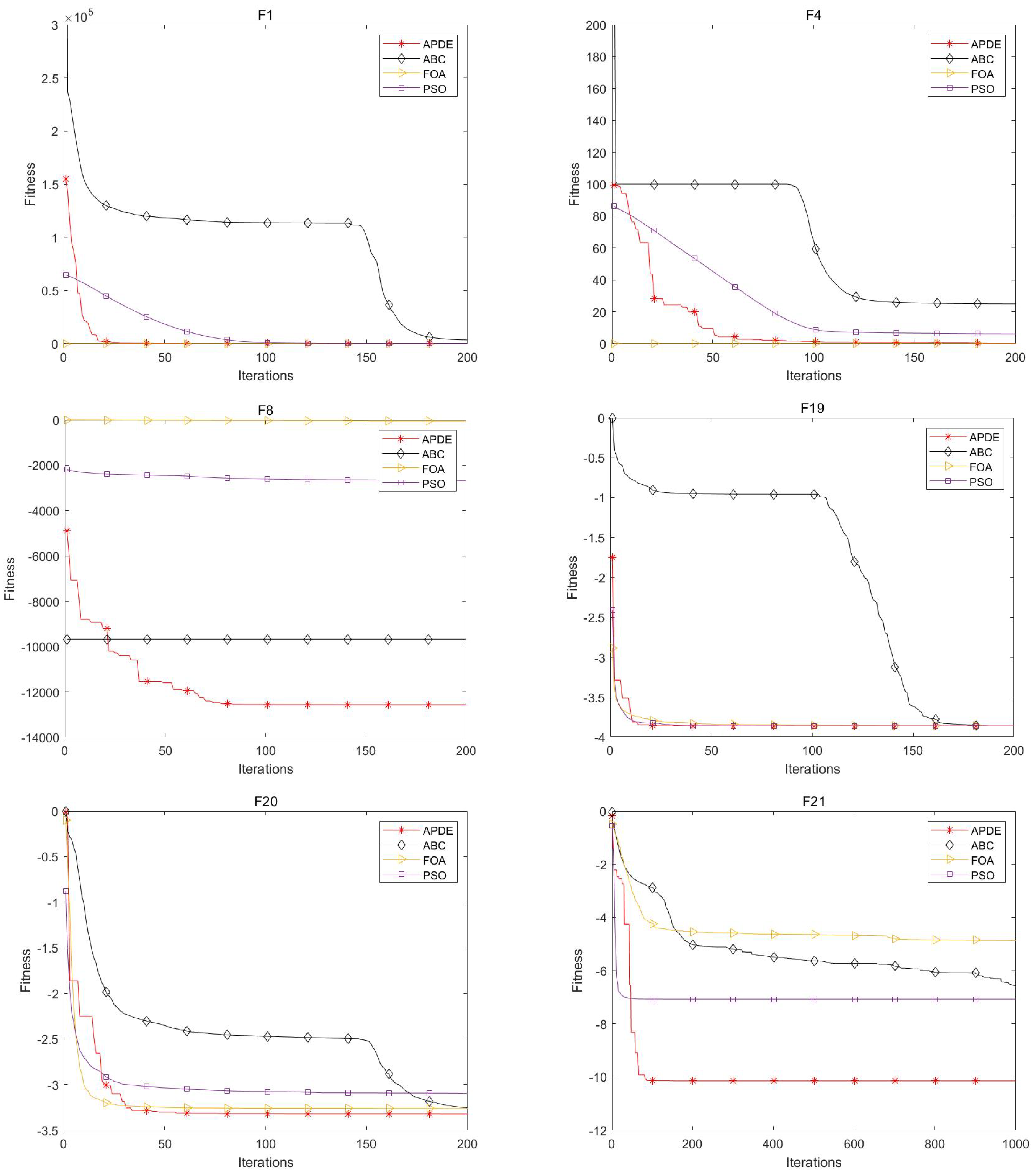
In Figure 5, the convergence curves of the three comparison algorithms with respect to test functions F1, F4, F8, F19, F20, and F21 in CEC2005 are presented. It can be seen from the figure that APDE can not only converge more quickly but also finds better solutions compared to other algorithms. On F1 and F4, the APDE converges second only to the FOA, which is due to the fact that the initial fitness value of the FOA is more close to the optimal solution 0. With respect to F8, F19, F20, and F21, the optimal value of the test function is negative, and the FOA has no initial solution advantage. At this point, APDE achieves the fastest convergence rate, as well as the smallest fitness value, through its powerful global exploration capability.
In Figure 6, the convergence curves of the three comparison algorithms on test functions F1, F5, F9, F22, F24, and F28 with respect to CEC2017 are presented. APDE has a unique two-stage structure and a mutation strategy that is more conducive to global search. Then, APDE is able to jump out of the current search region after briefly falling into a local optimum, which enhances the vitality of the algorithm. As can be seen in Figure 6, APDE has the fastest convergence rate, as well as the optimal fitness value, especially for F22. After APDE and PSO fall into a local optimum at the same node, PSO slowly stops updating the optimal solution, whereas APDE obtains a secondary search capability by jumping out of the current search region.

4.3. Wilcoxon Signed-Rank Test

To further analyze the performance of APDE, the Wilcoxon signed rank test is employed in this paper to compare the experimental results of CEC2005 and CEC2017 provided by APDE and other algorithms in a two-by-two manner. The Wilcoxon signed-rank test adds the ranks of the absolute values of the difference between the observed values and the center of the null hypothesis according to different signs as its test statistic. It suits paired comparisons without needing the differences between pairs of data to be normally distributed. From Table A3 and Table A4 in the Appendix B, we give the results of the significance comparisons based on the Wilcoxon signed rank test with p l e v e l = 0.5 . The comparison results are represented as (+, =, -) in the last row of Table A3 and Table A4. Here, (+) indicates that APDE is statistically superior to the comparison algorithms on current benchmark functions. (=) indicates that APDE is statistically neck-to-neck relative to the effect of the correlation comparison algorithm. (-) indicates that APDE does not perform better than the competition algorithms with respect to the current benchmark function.
The Wilcoxon signed-rank test results on the CEC2005 test set can be expressed as follows: CoDE (15,7,1), DE (15,6,2), BDE (16,7,0), JADE (16,4,3), NSDE (19,3,1), SaDE (16,5,2), FOA (21,0,2), PSO (21,2,0), and ABC (19,2,2). APDE outperforms the comparison algorithm in solving 158 of the 207 standardized test functions of CEC2005, and it performs statistically neck-to-neck relative to the comparison algorithm with respect to 36 functions.
The results on CEC2017 are: CoDE (29,0,0), DE (27,0,2), BDE (26,0,3), JADE (24,0,5), NSDE (21,0,8), SaDE (22,0,7), FOA (29,0,0), PSO (26,0,3), ABC (29,0,0). Here APDE outperforms the comparison algorithm in solving 233 of the 261 standardized test functions, and performs statistically worse than the comparison algorithm on only 28 functions.

4.4. Computational Complexity Analysis

The time complexity of APDE and the other comparison algorithms in this paper is O ( 1000 × D × N ) . Therefore, to deeply analyze the computational complexity of APDE, Table 7 provides the execution times of each algorithm running 20,000 times on CEC2017’s F18. The table indicates that the computational speed of APDE is surpassed by only PSO among the 10 algorithms evaluated, a circumstance that may be attributed to the simplistic architecture of PSO. Nevertheless, the employment of PSO necessitates a considerable investment of latent time dedicated to the fine-tuning of parameters. It can be observed from Figure 7 that APDE exhibits stability across problems of varying dimensions, with its runtime not significantly altering with an increase in dimensionality. This further validates the advantage of APDE in addressing high-dimensional problems.

5. Conclusions

Traditional DE-type algorithms are all parametric, which often need a lengthy process of parameter tuning, especially in solving different models to guarantee accuracy. Additionally, few of the current algorithms have been designed to take into account the characteristics of the iterative process. These may lead to an inadequate equilibrium between the efficiency and accuracy of the algorithm.
This paper proposes a two-stage adaptive differential evolutionary algorithm with accompanying populations, which develops different mutation strategies based on the search characteristics of each stage in the algorithm. APDE divides the search process into two phases by analyzing the search features, giving the calculation of adaptive weight factors and crossover factors with new distributional characteristics and balancing local searches and global exploration through population classification. Therefore, APDE can both converge quickly in the early stage and avoid falling into local optima in the later search stage.

Author Contributions

Conceptualization, C.M. and M.Z.; methodology, C.M. and M.Z.; software, M.Z.; validation, L.Z.; formal analysis, C.M. and M.Z.; resources, Q.Z. and Z.J.; data curation, Q.Z.; writing—original draft preparation, M.Z.; writing—review and editing, C.M.; visualization, M.Z.; supervision, L.Z. All authors have read and agreed to the published version of the manuscript.

Funding

This research received no external funding.

Data Availability Statement

No new data were created or analyzed in this study.

Conflicts of Interest

The authors declare no conflicts of interest.

Abbreviations

The following abbreviations are used in this manuscript:
APDEA two-stage adaptive differential evolution algorithm with accompanying populations;
DEDifferential evolution algorithm;
BDEBernstein–Levy differential evolution algorithm.

Appendix A. Test Function Information

Table A1. Uni-modal benchmark functions.
FunctionsDimensionsRange f min
F 1 = i = 1 n x i 2 30 100 , 100 0
F 2 = i = 0 n x i + i = 0 n x i 30 10 , 10 0
F 3 = i = 1 d j = 1 i x j 2 30 100 , 100 0
F 4 = max x i , 1 i n 30 100 , 100 0
F 5 = i = 1 n 1 100 x i 2 x i + 1 + 1 x i 2 30 30 , 30 0
F 6 = i = 1 n x i + 0.5 2 30 100 , 100 0
F 7 = i = 0 n i x i 4 + r a n d 0 , 1 30 128 , 128 0
F 8 = i = 1 n x i sin x i 30 500 , 500 12 , 569.5
F 9 = i = 1 n x i 2 10 cos 2 π x i + 10 30 5.12 , 5.12 0
F 10 = 20 exp 0.2 1 n i = 1 n x i 2 exp 1 n i = 1 n cos 2 π x i + 20 + e 30 32 , 32 0
F 11 = 1 + 1 4000 i = 1 n x i 2 i = 1 n cos x i i 30 600 , 600 0
F 12 = π n 10 sin π y 1 + i = 1 n 1 y i 1 2 1 + 10 sin 2 π y i + 1 + i = 1 n u x i , 10 , 100 , 4 30 50 , 50 0
where y i = 1 + x i + 1 4 , u x i , a , k , m K x i a m x i > a 0 a x i a K x i a m a x i
F 13 = 0.1 sin 2 3 π x 1 + i = 1 n x i 1 2 1 + sin 2 3 π x i + 1 + x n 1 2 1 + sin 2 3 π x n + i = 1 n u x i , 5 , 100 , 4 30 50 , 50 0
F 14 = 1 500 + j = 1 25 1 j + i = 1 2 x i a i , j 6 1 2 65 , 65 1
F 15 = i = 1 11 a i x 1 b i 2 + b i x 2 b i 2 + b i x 3 + x 4 2 4 5 , 5 0.003075
F 16 = 4 x 1 2 2.1 x 1 4 + 1 3 x 1 6 + x 1 x 2 4 x 2 2 + 4 x 2 4 2 5 , 5 1.0316285
F 17 = x 2 5.1 4 π 2 x 1 2 + 5 π x 1 6 2 + 10 1 1 8 π cos x 1 + 10 2 5 , 5 0.398
F 18 = 1 + x 1 + x 2 + 1 2 19 14 x 1 + 3 x 1 2 14 x 2 + 6 x 1 x 2 + 3 x 2 2 × 30 + 2 x 1 3 x 2 2 18 32 x 1 + 12 x 1 2 + 48 x 2 36 x 1 x 2 + 27 x 2 2 2 2 , 2 3
F 19 = i = 1 4 c i exp j = 1 3 a i j x j p i j 2 3 0 , 1 3.8628
F 20 = i = 1 4 c i exp j = 1 6 a i j x j p i j 2 6 0 , 1 0.32
F 21 = i = 1 5 X a i X a i T + c i 1 4 0 , 1 10.1532
F 22 = i = 1 7 X a i X a i T + c i 1 4 0 , 1 10.4028
F 23 = i = 1 10 X a i X a i T + c i 1 4 0 , 1 10.5363
Table A2. CEC2017 standard test functions.
No.Functions F i * = F i ( x * )
Unimodal Functions1Shifted and Rotated Bent Cigar Function100
3Shifted and Rotated Zakharov Function300
4Shifted and Rotated Rosenbrock Function400
5Shifted and Rotated Rastrigin Function500
6Shifted and Rotated Expanded Scaffer F6 Function600
Simple Multimodal Functions7Shifted and Rotated Lunacek Bi-Rastrigin Function700
8Shifted and Rotated Non-Continuous Rastrigin Function800
9Shifted and Rotated Levy Function900
10Shifted and Rotated Schwefel Function1000
Hybrid Functions11Hybrid Function 11100
12Hybrid Function 21200
13Hybrid Function 31300
14Hybrid Function 41400
15Hybrid Function 51500
16Hybrid Function 61600
17Hybrid Function 61700
18Hybrid Function 61800
19Hybrid Function 61000
20Hybrid Function 62000
Composition Functions21Composition Function 12100
22Composition Function 22200
23Composition Function 32300
24Composition Function 42400
25Composition Function 52500
26Composition Function 62600
27Composition Function 72700
28Composition Function 82800
29Composition Function 92900
30Composition Function 103000
D = 30; Search Range: [ 100 , 100 ] D

Appendix B. Wilcoxon Signed-Rank Test Results

Table A3. Wilcoxon signed-rank test results for CEC2005.
FncCoDEDE
R+R−p-ValueSig.R+R−p-ValueSig.
F10465 3.02 × 10 11 +51414 9.83 × 10 8 +
F20465 3.02 × 10 11 +35430 7.74 × 10 6 +
F30465 3.02 × 10 11 +0465 3.02 × 10 11 +
F40465 3.02 × 10 11 +0465 3.02 × 10 11 +
F50465 3.02 × 10 11 +0465 3.02 × 10 11 +
F60465 3.02 × 10 11 +853800.002+
F70465 3.02 × 10 11 +0465 3.02 × 10 11 +
F80465 3.02 × 10 11 +0465 3.02 × 10 11 +
F90465 3.02 × 10 11 +0465 3.02 × 10 11 +
F100465 3.02 × 10 11 +13452 1.1 × 10 8 +
F110465 3.02 × 10 11 +1772880.0392+
F120465 3.02 × 10 11 +0465 3.02 × 10 11 +
F130465 3.02 × 10 11 +28437 1.03 × 10 6 +
F14000=010.3337
F150465 2.49 × 10 7 +0360.0028+
F16000=000=
F17000=000=
F1804650.0055+000.0055+
F19000=000=
F201922730.31661562220.2145
F21000=000=
F22000=000=
F23000=000=
+ 15 15
= 7 6
1 2
FncBDEJADE
R+R−p-ValueSig.R+R−p-ValueSig.
F10465 3.02 × 10 11 +4650 3.02 × 10 11 +
F20465 3.02 × 10 11 +4650 3.02 × 10 11 +
F30465 3.02 × 10 11 +0465 3.02 × 10 11 +
F40465 3.02 × 10 11 +3471180.0232+
F50465 3.02 × 10 11 +0465 3.02 × 10 11 +
F60465 3.02 × 10 11 +4650 3.02 × 10 11 +
F70465 3.34 × 10 11 +0465 3.02 × 10 11 +
F80465 3.02 × 10 11 +0465 3.02 × 10 11 +
F90465 3.02 × 10 11 +0465 3.02 × 10 11 +
F100465 3.02 × 10 11 +300165 4.65 × 10 5 4+
F110465 3.02 × 10 11 +1832820.1079
F120465 3.02 × 10 11 +2352300.007+
F130465 3.02 × 10 11 +325140 9.51 × 10 6 +
F14000=000=
F150153 1.21 × 10 12 +030.1607
F16000=000=
F17000=000=
F18000.0055+000.0055+
F19000=000=
F204650 1.21 × 10 12 +39045 2.73 × 10 9 +
F21000=0100.0419+
F22000=0100.0419+
F23000=030.1608
+ 16 16
= 7 4
0 3
FncNSDESaDE
R+R−p-ValueSig.R+R−p-ValueSig.
F10465 5.07 × 10 10 +4650 3.02 × 10 11 +
F240956 3.81 × 10 7 +4650 3.02 × 10 11 +
F30465 3.02 × 10 11 +0465 3.02 × 10 11 +
F40465 3.02 × 10 11 +0465 3.02 × 10 11 +
F50465 3.02 × 10 11 +0465 3.02 × 10 11 +
F612453 5.46 × 10 9 +4650 3.02 × 10 11 +
F70465 3.02 × 10 11 +0465 6.07 × 10 11 +
F80465 3.02 × 10 11 +0465 3.02 × 10 11 +
F90465 3.02 × 10 11 +0465 3.02 × 10 11 +
F100465 3.02 × 10 11 +43530 5.54 × 10 10 +
F1111454 4.18 × 10 9 +2642010.0035+
F120465 3.02 × 10 11 +43530 5.57 × 10 10 +
F130465 3.02 × 10 11 +37887 1.07 × 10 7 +
F1404650.0215+000=
F150465 6.36 × 10 5 +030.1608
F16000=000=
F17000=000=
F1804650.0055+000.0055+
F19000=000=
F202332320.085837590 3.75 × 10 6 +
F213511140.0419+0100.0419+
F222761890.0055+030.1607
F232102550.000658+000=
+ 19 16
= 3 5
1 2
FncFOAPSO
R+R−p-ValueSig.R+R−p-ValueSig.
F10465 3.02 × 10 11 +0465 3.02 × 10 11 +
F20465 3.02 × 10 11 +0465 3.02 × 10 11 +
F32292360.3790465 3.02 × 10 11 +
F4411540.000399+0465 3.02 × 10 11 +
F50465 3.02 × 10 11 +0465 3.02 × 10 11 +
F60465 3.02 × 10 11 +0465 3.02 × 10 11 +
F713452 1.55 × 10 9 +0465 3.02 × 10 11 +
F80465 3.02 × 10 11 +0465 3.02 × 10 11 +
F90465 3.02 × 10 11 +0465 3.02 × 10 11 +
F100465 3.02 × 10 11 +0465 3.02 × 10 11 +
F114614 8.48 × 10 9 +0465 3.02 × 10 11 +
F120465 3.02 × 10 11 +0465 3.02 × 10 11 +
F130465 3.02 × 10 11 +0465 3.02 × 10 11 +
F140465 3.02 × 10 11 +04650.0056+
F150465 1.21 × 10 12 +04650.0216+
F160465 1.21 × 10 12 +000=
F170465 1.21 × 10 12 +000=
F180465 7.57 × 10 12 +04650.0055+
F190465 1.21 × 10 12 +3511140.0418+
F202801850.2905444210.000156+
F210465 1.21 × 10 12 +153312 6.13 × 10 5 +
F220465 1.21 × 10 12 +1712940.000144+
F230465 1.21 × 10 12 +136329 2.9 × 10 5 +
+ 21 21
= 0 2
2 0
FncABC
R+R−p-ValueSig.
F10465 3.02 × 10 11 +
F20465 3.02 × 10 11 +
F30465 3.02 × 10 11 +
F40465 3.02 × 10 11 +
F50465 3.02 × 10 11 +
F60465 3.02 × 10 11 +
F70465 6.7 × 10 11 +
F81464 5.57 × 10 10 +
F90465 3.02 × 10 11 +
F100465 3.02 × 10 11 +
F110465 3.02 × 10 11 +
F120465 3.02 × 10 11 +
F130465 3.02 × 10 11 +
F14000=
F150465 8.99 × 10 11 +
F1604651
F1704651
F1804650.0055+
F19000=
F2039273 6.04 × 10 7 +
F2145420 2.1 × 10 8 +
F2266399 8.78 × 10 8 +
F23105360 4.27 × 10 6 +
+ 19
= 2
2
Table A4. Wilcoxon signed-rank test results for CEC2017.
FncCoDEDE
R+R−p-ValueSig.R+R−p-ValueSig.
F10465 3.02 × 10 11 +26439 2.88 × 10 6 +
F30465 3.02 × 10 11 +0465 3.02 × 10 11 +
F427438 6.77 × 10 5 +3611040.0798
F50465 4.98 × 10 11 +0465 3.02 × 10 11 +
F60465 3.02 × 10 11 +4578 8.1 × 10 10 +
F72463 4.2 × 10 10 +0465 3.02 × 10 11 +
F80465 3.02 × 10 11 +0465 3.02 × 10 11 +
F90465 3.02 × 10 11 +4650 3.02 × 10 11 +
F1043233 9.26 × 10 9 +70395 5.27 × 10 5 +
F110465 3.02 × 10 11 +6459 5.09 × 10 8 +
F120465 3.02 × 10 11 +6459 8.1 × 10 10 +
F130465 3.02 × 10 11 +0465 3.82 × 10 10 +
F144614 8.48 × 10 9 +4623 7.77 × 10 9 +
F15398670.0037+4650 1.61 × 10 10 +
F1624441 8.35 × 10 8 +0465 3.02 × 10 11 +
F177458 2.67 × 10 9 +7458 3.2 × 10 9 +
F1846419 5.46 × 10 6 +379860.000422+
F19393720.0083+4623 7.38 × 10 10 +
F20953700.002+973680.0028+
F210465 3.02 × 10 11 +0465 3.02 × 10 11 +
F229456 1.07 × 10 9 +8457 7.6 × 10 7 +
F230465 3.02 × 10 11 +0465 3.02 × 10 11 +
F240465 3.02 × 10 11 +0465 3.02 × 10 11 +
F254461 5.07 × 10 10 +41550 2.2 × 10 7 +
F260465 3.02 × 10 11 +0465 3.02 × 10 11 +
F2744124 1.11 × 10 6 +4569 2.23 × 10 9 +
F280465 3.02 × 10 11 +2582070.4204
F29843810.000189+8457 3.65 × 10 8 +
F3011454 7.38 × 10 10 +883770.0076+
+ 29 27
= 0 0
0 2
FncBDEJADE
R+R−p-ValueSig.R+R−p-ValueSig.
F10465 3.02 × 10 11 +4650 3.02 × 10 11 +
F33441210.0138+383820.000446+
F41163490.000104+4641 2.83 × 10 8 +
F53462 34.18 × 10 9 +1323330.0076+
F669396 2.6 × 10 5 +42243 2.49 × 10 6 +
F717448 2.32 × 10 6 +2901750.5692
F80465 3.02 × 10 11 +514140.000399+
F91293360.0014+4650 1.96 × 10 10 +
F104605 8.48 × 10 9 +4623 5 × 10 9 +
F114461 2.83 × 10 8 +1063590.007+
F125460 1.21 × 10 10 +43728 3.81 × 10 7 +
F130465 6.72 × 10 10 +2402250.3953
F142212440.69522871780.000239+
F15494160.000168+37986 1.19 × 10 6 +
F1635430 1.75 × 10 5 +1992660.2226
F1722443 8.35 × 10 8 +1393260.0076+
F182212440.76183331320.00077+
F19763890.000952+39966 1.25 × 10 7 +
F20833820.000399+1003650.0037+
F210465 3.02 × 10 11 +723930.0013+
F222891760.773140857 9.58 × 10 9 +
F230465 3.02 × 10 11 +1662990.1858
F240465 3.34 × 10 11 +1073580.0095+
F251633020.0224+366990.0012+
F26129336 7.74 × 10 6 +983670.0176+
F27793860.000168+3011640.1023
F281423230.0378+44223 1.39 × 10 6 +
F291513140.0281+1193460.0024+
F3040425 3.75 × 10 6 +3641010.000471+
+ 26 24
= 0 0
3 5
FncNSDESaDE
R+R−p-ValueSig.R+R−p-ValueSig.
F1604050.000158+4650 3.02 × 10 11 +
F3405600.00077+0465 1.61 × 10 10 +
F41902750.36322791860.4825
F550415 7.09 × 10 8 +0465 3.34 × 10 11 +
F60465 3.34 × 10 11 +4650 1.78 × 10 10 +
F735430 5.86 × 10 6 +0465 9.76 × 10 10 +
F89456 2.67 × 10 9 +0465 3.02 × 10 11 +
F915450 2.67 × 10 9 +4650 2.84 × 10 11 +
F104623 1.17 × 10 9 +2302350.5793
F11554100.000133+61404 4.35 × 10 5 +
F1225440 3.37 × 10 5 +793860.000253+
F137458 4.18 × 10 9 +0465 3.02 × 10 11 +
F143401250.0327+3331320.0364+
F151543110.18092781870.7172
F161513140.12246459 7.12 × 10 9 +
F1747418 2.13 × 10 5 +5460 5.46 × 10 9 +
F183571080.0127+16449 1.47 × 10 7 +
F191483170.0378+3161490.1055
F2037428 6.28 × 10 6 +47418 5.27 × 10 5 +
F219456 1.56 × 10 8 +0465 3.02 × 10 11 +
F22923730.06351782870.3478
F23344310.000129+0465 3.02 × 10 11 +
F240465 1.17 × 10 9 +0465 3.02 × 10 11 +
F251782870.20093281370.1023
F266459 2.92 × 10 9 +0465 3.02 × 10 11 +
F272072580.86544322 5.19 × 10 7 +
F281453200.06352282370.8418
F291413240.051927438 2.57 × 10 7 +
F30374910.0038+673980.000225+
+ 21 22
= 0 0
8 7
FncFOAPSO
R+R−p-ValueSig.R+R−p-ValueSig.
F10465 3.02 × 10 11 +0465 3.02 × 10 11 +
F30465 3.02 × 10 11 +1464 6.07 × 10 11 +
F40465 3.02 × 10 11 +0465 8.15 × 10 11 +
F50465 3.02 × 10 11 +0465 3.34 × 10 11 +
F60465 3.02 × 10 11 +0465 3.02 × 10 11 +
F70465 3.02 × 10 11 +0465 3.02 × 10 11 +
F80465 3.02 × 10 11 +0465 3.02 × 10 11 +
F90465 3.02 × 10 11 +0465 3.02 × 10 11 +
F100465 3.02 × 10 11 +2721930.3255
F110465 3.02 × 10 11 +1464 2.37 × 10 10 +
F120465 3.02 × 10 11 +0465 3.02 × 10 11 +
F130465 3.02 × 10 11 +0465 3.02 × 10 11 +
F140465 3.02 × 10 11 +1363290.0877
F150465 3.02 × 10 11 +60405 3.09 × 10 6 +
F160465 3.02 × 10 11 +3462 8.89 × 10 10 +
F170465 3.02 × 10 11 +0465 3.69 × 10 11 +
F180465 3.02 × 10 11 +1752900.1413
F190465 3.02 × 10 11 +634020.000239+
F200465 3.02 × 10 11 +0465 4.08 × 10 11 +
F210465 3.02 × 10 11 +0465 3.02 × 10 11 +
F220465 3.02 × 10 11 +0465 3.82 × 10 10 +
F230465 3.02 × 10 11 +0465 3.02 × 10 11 +
F240465 3.02 × 10 11 +0465 3.02 × 10 11 +
F250465 3.02 × 10 11 +0465 3.02 × 10 11 +
F260465 3.02 × 10 11 +10455 8.2 × 10 7 +
F270465 3.02 × 10 11 +0465 3.02 × 10 11 +
F280465 3.02 × 10 11 +0465 5.49 × 10 11 +
F290465 3.02 × 10 11 +0465 3.02 × 10 11 +
F300465 3.02 × 10 11 +0465 3.02 × 10 11 +
+ 29 26
= 0 0
3 0
FncABC
R+R−p-ValueSig.
F10465 3.02 × 10 11 +
F33401250.0138+
F40465 3.02 × 10 11 +
F50465 3.02 × 10 11 +
F60465 3.02 × 10 11 +
F70465 6.7 × 10 11 +
F81464 5.57 × 10 10 +
F90465 3.02 × 10 11 +
F1041451 4.11 × 10 7 +
F110465 3.02 × 10 11 +
F120465 3.02 × 10 11 +
F130465 3.02 × 10 11 +
F1437428 5.86 × 10 6 +
F150465 6.07 × 10 11 +
F160465 3.69 × 10 11 +
F170465 3.69 × 10 11 +
F18783870.00077+
F190465 3.69 × 10 11 +
F204461 2.61 × 10 10 +
F210465 3.02 × 10 11 +
F2245420 2.92 × 10 9 +
F230465 3.69 × 10 11 +
F240465 3.69 × 10 11 +
F250465 3.69 × 10 11 +
F260465 3.69 × 10 11 +
F270465 3.69 × 10 11 +
F280465 3.69 × 10 11 +
F290465 3.69 × 10 11 +
F300465 3.69 × 10 11 +
+ 29
= 0
0

References

  1. Zhang, A.; Shi, W. Mining significant fuzzy association rules with differential evolution algorithm. Appl. Soft Comput. 2020, 97, 1568–4946. [Google Scholar] [CrossRef]
  2. Wang, Z.; Tang, J.; Xia, H.; Zhang, X.; Jing; Han, H. Used mobile phone recognition method based on parallel differential evolution and gradient feature deep forest. Control Theory Appl. 2022, 39, 2137–2148. [Google Scholar]
  3. Feng, S.; Chen, L.; Liu, M. Random structure based design method for multiplierless IIR digital filters. J. Comput. Appl. 2018, 38, 2621–2625. [Google Scholar]
  4. Yılmaz, O.; Bas, E.; Egrioglu, E. The Training of Pi-Sigma Artificial Neural Networks with Differential Evolution Algorithm for Forecasting. Comput. Econ. 2022, 59, 1699–1711. [Google Scholar] [CrossRef]
  5. Dong, L.; Jiang, F.; Li, D.; Mladenovic, N. IP extraction from magnetotelluric sounding data based on adaptive differential evolution inversion. Oil Geophys. Prospect. 2016, 51, 613–624420. [Google Scholar]
  6. Wu, H.; Wang, Y.; Zhou, S.; Yuan, X. Research and application of pseudo parallel differential evolution algorithm with dual subpopulations. Control Theory Appl. 2007, 24, 453–458. [Google Scholar]
  7. He, Y.; Wang, X.; Liu, K.; Wang, Y. Convergent Analysis and Algorithmic Improvement of Differential Evolution. J. Softw. 2010, 21, 875–885. [Google Scholar] [CrossRef]
  8. Du, Y.; Fan, Y.; Liu, P.; Tang, J.; Luo, Y. Multi-populations Covariance Learning Differential Evolution Algorithm. J. Electron. Inf. Technol. 2019, 41, 1488–1495. [Google Scholar]
  9. Chen, Y.; Liu, S.; Zhang, Z. Multi-strategy Differential Evolutionary Algorithm Oriented by Excellent Individual. Comput. Eng. Appl. 2022, 58, 137–144. [Google Scholar]
  10. Ge, J.; Qi, R.; Qian, F.; Chen, J. A Modified Adaptive Differential Evolution Algorithm. J. East China Univ. Sci. Technol. (Nat. Sci. Ed.) 2009, 35, 600–605. [Google Scholar]
  11. Yao, F.; Yang, W.; Zhang, M.; Li, Z. Improved space-adaptive-based differential evolution algorithm. Control Theory Appl. 2010, 27, 32–38. [Google Scholar]
  12. Zhang, Y.; Tao, Y.; Wang, J. An Improved DE Algorithm for Solving Hybrid Flow-shop Scheduling Problems. China Mech. Eng. 2021, 32, 714–720. [Google Scholar]
  13. Wang, M.; Ma, Y.; Wang, P. Parameter and strategy adaptive differential evolution algorithm based on accompanying evolution. in Inf. Sci. 2022, 607, 1136–1157. [Google Scholar] [CrossRef]
  14. Huang, L.; Liu, S.; Gao, W. Differential evolution with the search strategy of artificial bee colony algorithm. Control Decis. 2012, 27, 1644–1648. [Google Scholar]
  15. Li, M.; Zhao, H.; Weng, X.; Han, T. Differential evolution based on optimal Gaussian random walk and individual selection strategies. Control Decis. 2016, 31, 1379–1386. [Google Scholar]
  16. Wang, L.; Zhang, G.; Zhou, X. Strategy Self-adaptive Differential Evolution Algorithm Based on State Estimation Feedback. Acta Autom. Sin. 2020, 46, 752–766. [Google Scholar]
  17. Fu, L.; Zhu, H.; Zhang, C.; Ouyang, H.; Li, S. Hybrid Harmony Search Differential Evolution Algorithm. IEEE Access 2021, 9, 21532–21555. [Google Scholar] [CrossRef]
  18. Huang, C.; Bai, H.; Yao, X. Online algorithm configuration for differential evolution algorithm. Appl. Intell. 2022, 52, 9193–9211. [Google Scholar] [CrossRef]
  19. Civicioglu, P.; Besdok, E. Bernstein-Levy differential evolution algorithm for numerical function optimization. Neural Comput. Appl. 2023, 35, 6603–6621. [Google Scholar] [CrossRef]
  20. Chen, J.; He, Q. Mixed Strategy to Improve Sparrow Search Algorithm. J. Chin. Comput. Syst. 2023, 44, 1470–1478. [Google Scholar]
  21. Hu, Z.; Xiong, S.; Su, Q.; Fang, Z. Finite Markov chain analysis of classical differential evolution algorithm. J. Comput. Appl. Math. 2014, 268, 121–134. [Google Scholar] [CrossRef]
  22. Ma, F.; Cai, G. Calculating an Infinite Limit with an Embedded Composite Function. Stud. Coll. Math. 2023, 26, 7–8. [Google Scholar]
  23. Dong, M.; Wang, N.; Chen, X. Improved Composite Differential Evolution Algorithms. Comput. Simul. 2013, 30, 389–392. [Google Scholar]
  24. Deng, L.; Qin, Y.; Li, C.; Zhang, L. An adaptive mutation strategy correction framework for differential evolution. Neural Comput. Appl. 2023, 35, 11161–11182. [Google Scholar] [CrossRef]
  25. Zhang, J.; Sanderson, A. JADE: Adaptive Differential Evolution With Optional External Archive. IEEE Trans. Evol. Comput. 2009, 13, 945–958. [Google Scholar] [CrossRef]
  26. Psychas, I.; Marinaki, M.; Marinakis, Y.; Migdalas, A. Non-dominated sorting differential evolution algorithm for the minimization of route based fuel consumption multiobjective vehicle routing problems. Energy Syst. 2017, 8, 785–814. [Google Scholar] [CrossRef]
  27. Zhu, L.; Ma, Y.; Bai, Y. A self-adaptive multi-population differential evolution algorithm. Nat. Comput. 2020, 19, 211–235. [Google Scholar] [CrossRef]
  28. Ehsaeyan, E.; Zolghadrasli, A. FOA: Fireworks optimization algorithm. Multimed. Tools Appl. 2022, 81, 33151–33170. [Google Scholar] [CrossRef]
  29. Wang, Q.; Zhang, B.; Ouyang, A.; Xu, G. Cross strategy particle swarm optimization. J. Southwest China Norm. Univ. Sci. Ed. 2022, 47, 57–62. [Google Scholar]
  30. Zhou, S.; Kong, J.; Hou, Y.; Zou, G. Multi-objective Optimization of Tandem Robot with Improved ABC Algorithm. Modul. Mach. Tool Autom. Manuf. Tech. 2019, 5, 31–35. [Google Scholar]
Figure 1. Schematic diagram of the two-stage strategy with accompanying populations.
Mathematics 13 00440 g001
Figure 2. Schematic diagram of the improved mutation operator.
Mathematics 13 00440 g002
Figure 3. Function convergence curves of DE-type algorithms with respect to CEC2005.
Mathematics 13 00440 g003
Figure 4. Function convergence curves of DE-type algorithms with respect to CEC2017.
Mathematics 13 00440 g004
Figure 5. Function convergence curves of APDE and non-DE algorithms on CEC2005.
Mathematics 13 00440 g005
Figure 6. Function convergence curves of APDE and non-DE algorithms on CEC2017.
Mathematics 13 00440 g006
Figure 7. Runtimes of various algorithms on the F18 benchmark.
Mathematics 13 00440 g007
Table 1. Initial values of the related parameters used in DE-type algorithms.
AlgorithmInitial Values of the Related Parameters
1CoDE N = 30 , F = [ 1.0 1.0 0.8 ] , and  C R = [ 0.1 0.9 0.2 ]
2BDE N = 30
3JADE N = 30 , F = 0.5 , C R = 0.5 , and  p 0 = 0.1
4SADE C R ( 0.5 , 0.1 ) , F ( 0.4 , 0.003333 ) , and i k u n i = 0.25 ( i = 1 , 2 , 3 , 4 )
5DE N = 30 , F = 0.6 , and  C R = 0.8
Table 2. Experimental results of DE-type algorithms with respect to CEC2005.
APDECoDEDEBDEJADENSDESaDE
F1Mean 2.0111 × 10 5 5.9860 × 10 1 3.4653 × 10 5 6.6900 × 10 2 1.8312 × 10 29 5.2000 × 10 2 1.4692 × 10 22
Std 2.4701 × 10 5 1.7170 × 10 1 5.7341 × 10 5 4.5200 × 10 2 8.0982 × 10 29 2.6350 × 10 1 8.0112 × 10 22
F2Mean 1.3000 × 10 3 1.3970 × 10 1 4.9000 × 10 3 7.5400 × 10 2 1.7680 × 10 16 7.4564 × 10 4 4.9802 × 10 13
Std 8.7158 × 10 4 3.5500 × 10 2 2.3000 × 10 3 2.3500 × 10 2 2.3758 × 10 16 1.7000 × 10 3 1.3189 × 10 12
F3Mean 1.4930 × 10 1 2.0261 × 10 4 5.9992 × 10 3 5.207021 × 10 2 5.9828 1.974929 × 10 2 5.905769 × 10 2
Std 1.5820 × 10 1 2.6561 × 10 3 1.9340 × 10 3 2.841297 × 10 2 3.6729 9.50277 × 10 1 5.814403 × 10 2
F4Mean 1.2400 × 10 2 3.75102 × 10 1 8.55992.2086 9.7000 × 10 3 3.9982 × 10 1 2.3680
Std 1.3200 × 10 2 3.02284.8623 7.25500 × 10 1 8.3000 × 10 3 6.13351.5353
F5Mean 4.4316 × 10 4 4.453352 × 10 2 3.41989 × 10 1 7.08419 × 10 1 1.34262 × 10 1 2.043849 × 10 2 3.27313 × 10 1
Std 4.8201 × 10 4 9.62976 × 10 1 2.15395 × 10 1 4.66516 × 10 1 1.23849 × 10 1 1.551284 × 10 2 2.41183 × 10 1
F6Mean 1.9954 × 10 5 6.0020 × 10 1 4.8356 × 10 5 6.9100 × 10 2 1.6210 × 10 29 1.1180 × 10 1 8.8471 × 10 25
Std 3.1580 × 10 5 2.2910 × 10 1 3.2976 × 10 5 4.4700 × 10 2 4.8882 × 10 29 4.5750 × 10 2 2.5111 × 10 24
F7Mean 2.0000 × 10 3 8.0680 × 10 1 3.1200 × 10 2 3.5700 × 10 2 7.1716 × 10 2 2.1490 × 10 1 1.1200 × 10 2
Std 9.7877 × 10 4 2.1410 × 10 1 8.4000 × 10 3 1.3300 × 10 2 3.4930 × 10 2 1.0650 × 10 1 4.4850 × 10 3
F8Mean 1.2569 × 10 4 1.2359 × 10 4 6.4519 × 10 3 1.2519 × 10 4 9.88444 × 10 3 9.2891 × 10 3 1.0362 × 10 4
Std 4.5000 × 10 3 1.508268 × 10 2 5.33804 × 10 2 6.10444 × 10 1 3.037302 × 10 2 6.812488 × 10 2 1.4838 × 10 3
F9Mean 2.5615 × 10 5 1.4697 × 10 1 1.927408 × 10 2 2.39388 × 10 1 1.86455 × 10 1 3.97028 × 10 1 1.050872 × 10 2
Std 3.3880 × 10 5 2.5241 1.41917 × 10 1 3.36262.6113 1.04575 × 10 1 1.43169 × 10 1
F10Mean 9.4246 × 10 4 1.70904 × 10 1 6.3566 8.1100 × 10 2 1.3910 × 10 1 1.41083 × 10 1 1.3340 × 10 13
Std 7.5380 × 10 4 5.82149.1827 1.9400 × 10 2 3.6308 × 10 1 5.9864 1.6936 × 10 13
F11Mean 5.5418 × 10 4 7.5300 × 10 1 3.3000 × 10 3 2.1770 × 10 1 4.9899 × 10 3 1.4640 × 10 1 2.5457 × 10 3
Std 2.6000 × 10 3 1.0630 × 10 1 9.2000 × 10 3 9.6300 × 10 2 1.2366 × 10 2 4.0030 × 10 1 4.9465 × 10 3
F12Mean 1.4094 × 10 7 2.2710 × 10 1 4.7075 × 10 5 5.8715 × 10 4 1.3866 × 10 2 1.2814 3.4556 × 10 3
Std 3.8140 × 10 7 1.1530 × 10 1 8.1738 × 10 5 5.4181 × 10 4 4.4994 × 10 2 2.4849 1.8927 × 10 2
F13Mean 2.1444 × 10 6 6.8000 × 10 2 7.0836 × 10 6 4.5000 × 10 3 1.0987 × 10 3 6.9840 × 10 1 1.1990 × 10 1
Std 1.1358 × 10 6 2.4500 × 10 2 3.2267 × 10 6 3.0000 × 10 3 3.3526 × 10 3 2.4797 6.5680 × 10 1
F14Mean 9.9800 × 10 1 9.9800 × 10 1 1.0974 9.9800 × 10 1 9.9800 × 10 1 1.32791.0643
Std00 3.0330 × 10 1 00 9.8170 × 10 1 2.5220 × 10 1
F15Mean 3.0749 × 10 4 1 × 10 3 1.7 × 10 3 3.075 × 10 4 3.685 × 10 4 1.4 × 10 3 3 × 10 3
Std 1.9206 × 10 19 5.0063 × 10 4 5.1 × 10 3 1.5907 × 10 8 2.3232 × 10 4 3.6 × 10 3 6.9 × 10 3
F16Mean 1.0316 −1.0316−1.0316−1.0316−1.0316−1.0316−1.0316
Std 6.3208 × 10 16 6.7752 × 10 16 6.7752 × 10 16 6.3532 × 10 16 6.7752 × 10 16 6.7752 × 10 16 6.7752 × 10 16
F17Mean 3.979 × 10 1 3.979 × 10 1 3.979 × 10 1 3.979 × 10 1 3.979 × 10 1 3.979 × 10 1 3.979 × 10 1
Std0000000
F18Mean3333333
Std 4.7536 × 10 15 1.3550 × 10 15 1.9375 × 10 15 4.0803 × 10 15 1.9946 × 10 15 1.1865 × 10 15 2.1615 × 10 15
F19Mean−3.8628−3.8628−3.8628−3.8628−3.8628−3.8628−3.8628
Std 2.5973 × 10 15 2.7101 × 10 15 7.3446 × 10 15 7.1201 × 10 15 2.7101 × 10 15 2.7101 × 10 15 2.7101 × 10 15
F20Mean−3.2625−3.2269−3.219−3.322−3.2943−3.2388−3.2665
Std 6.0500 × 10 2 4.8400 × 10 2 4.1100 × 10 2 1.4729 × 10 15 5.1146 × 10 2 5.54 × 10 2 6.03 × 10 2
F21Mean 1.01532 × 10 1 1.01532 × 10 1 −9.9833 1.01532 × 10 1 −9.3972−9.475−9.485
Std 3.3404 × 10 15 6.9584 × 10 15 9.308 × 10 1 5.627 × 10 15 2.00021.75872.0722
F22Mean 1.04029 × 10 1 1.04029 × 10 1 1.04029 × 10 1 1.04029 × 10 1 1.01803 × 10 1 −9.1173 1.02258 × 10 1
Std 1.0881 × 10 16 1.2342 × 10 15 1.1427 × 10 15 3.2986 × 10 16 1.21932.3819 9.704 × 10 1
F23Mean 1.05364 × 10 1 1.05364 × 10 1 1.05364 × 10 1 1.05364 × 10 1 1.05364 × 10 1 −8.4124 1.03577 × 10 1
Std 1.4752 × 10 15 1.8067 × 10 15 3.2643 × 10 15 2.7202 × 10 15 1.8067 × 10 15 3.0976 9.787 × 10 1
Table 3. Experimental results of DE-type algorithms with respect to CEC2017.
APDECoDEDEBDEJADENSDESaDE
F1Mean3140 8.3196 × 10 6 1.5296 × 10 4 5.4656 × 10 5 100.1182120,980113.433
Std2371.8 1.9186 × 10 6 1.4744 × 10 4 2.7159 × 10 5 0.18915595,29024.0785
F3Mean50,653 1.4192 × 10 5 1.4044 × 10 5 4.2345 × 10 4 3540239,22596,478
Std11,710 1.9977 × 10 4 2.1116 × 10 4 1.3805 × 10 4 16,72412,52622,086
F4Mean496.3799 5.204201 × 10 2 4.882713 × 10 2 5.135177 × 10 2 443.0121508.0222493.96
Std23.9316 1.32951 × 10 1 1.1872 1.6671 × 10 1 34.180335.864712.9516
F5Mean549.3403 6.639587 × 10 2 7.160121 × 10 2 6.226352 × 10 2 553.2752584.1904680.6822
Std27.9434 1.13691 × 10 1 1.26556 × 10 1 1.44561 × 10 1 13.11726.417412.5815
F6Mean600.5493 6.028136 × 10 2 6.001868 × 10 2 6.008292 × 10 2 600.2091606.629600.0182
Std0.3261 4.337 × 10 1 1.057 × 10 1 2.988 × 10 1 0.294125.28150.0996
F7Mean801.3148 9.23662 × 10 2 9.550189 × 10 2 8.763957 × 10 2 782.657854.0382915.6208
Std47.8577 1.68969 × 10 1 1.17354 × 10 1 1.57737 × 10 1 9.399334.160913.6573
F8Mean837.7225 9.74909 × 10 2 1.0221 × 10 3 9.243664 × 10 2 847.5331874.735975.4408
Std9.9356 1.42838 × 10 1 1.03089 × 10 1 1.00326 × 10 1 9.090423.008414.229
F9Mean967.2169 4.0333 × 10 3 9.010213 × 10 2 1.0038 × 10 3 904.72971447.7900.3961
Std82.7747 7.788275 × 10 2 7.331 × 10 1 9.09459 × 10 1 8.6947429.18110.5461
F10Mean7794.9 6.14 × 10 3 8.469 × 10 3 5.3364 × 10 3 4614.64553.87865.7
Std1085.7 3.341728 × 10 2 3.581 × 10 2 3.330016 × 10 2 742.8817875.5873659.3392
F11Mean1177.7 1.2997 × 10 3 1.2381 × 10 3 1.2466 × 10 3 1205.71224.81219.5
Std37.373 1.71649 × 10 1 2.1279 × 10 1 3.34554 × 10 1 36.04575647.292529.6147
F12Mean123,480 2.668 × 10 7 2.3824 × 10 6 1.276 × 10 6 32,856479,990596,300
Std155,350 6.2779 × 10 6 3.436 × 10 6 9.0697 × 10 5 26,573811,2501.1177
F13Mean2519 1.3822 × 10 4 1.3419 × 10 4 1.7272 × 10 4 3193.124,40839,356
Std946.358 4.3167 × 10 3 1.1755 × 10 4 1.3849 × 10 4 3417.621,20726,625
F14Mean3313.3 1.5042 × 10 3 1.4963 × 10 3 3.1815 × 10 3 7251.92274.12336.6
Std2501.5 1.02349 × 10 1 9.3189 1.981 × 10 3 15,2891549.41583.7
F15Mean3489.3 1.8207 × 10 3 1.6517 × 10 3 7.1935 × 10 3 1993.27235.42368.5
Std2859.3 4.02862 × 10 1 3.87281 × 10 1 5.4051 × 10 3 1080.310,222550.5201
F16Mean2326.9 2.7748 × 10 3 3.3051 × 10 3 2.6774 × 10 3 2387.12448.72866.5
Std298.5276 1.576967 × 10 2 1.67845 × 10 2 2.371197 × 10 2 180.9872276.2654201.866
F17Mean1825.1 2.0855 × 10 3 2.2338 × 10 3 2.0229 × 10 3 1866.92009.82061.9
Std100.5111 1.103453 × 10 2 2.317953 × 10 2 1.279731 × 10 2 82.6965204.7595.2961
F18Mean88,453 1.7984 × 10 5 4.5786 × 10 4 9.2897 × 10 4 65,55358,304562,850
Std57,972 9.6414 × 10 4 2.6365 × 10 4 6.1834 × 10 4 104,79041,686459,140
F19Mean3835.5 2.198 × 10 3 1.958 × 10 3 8.1099 × 10 3 2583.16798.22958.9
Std2509.9 1.206883 × 10 2 1.29483 × 10 1 7.5543 × 10 3 2262.66656.42186.6
F20Mean2214.6 2.3514 × 10 3 2.396 × 10 3 2.3442 × 10 3 2287.32414.92369
Std140.867 1.794837 × 10 2 2.467335 × 10 2 1.238921 × 10 2 77.3064148.0423123.7216
F21Mean2339.8 2.4676 × 10 3 2.5102 × 10 3 2.4217 × 10 3 2350.42368.52470.5
Std13.3063 1.34699 × 10 1 1.27128 × 10 1 1.60098 × 10 1 10.261514.99416.1366
F22Mean2661.1 6.8675 × 10 3 8.2854 × 10 3 2.3038 × 10 3 2543.34502.14974.6
Std1387 1.6838 × 10 3 3.0569 × 10 3 2.4445 × 10 3 927.71521890.33433.5
F23Mean2702.3 2.8077 × 10 3 2.8574 × 10 3 2.7709 × 10 3 2707.42737.12829.4
Std14.2395 1.26972 × 10 1 1.48102 × 10 1 1.35514 × 10 1 13.650433.287221.7018
F24Mean2863.4 3.0085 × 10 3 3.0263 × 10 3 2.9508 × 10 3 28732921.73009.8
Std11.0091 1.76891 × 10 1 1.18241 × 10 1 3.02613 × 10 1 15.293240.489515.1783
F25Mean2894.5 2.92840 × 10 3 2.8872 × 10 3 2.8976 × 10 3 2887.62901.12889.5
Std10.3697 1.2405 × 10 1 1.249 × 10 1 1.03817 × 10 1 1.554721.39294.8153
F26Mean4174.7 5.3037 × 10 3 5.7368 × 10 3 4.6578 × 10 3 4335.247685356.7
Std303.6389 1.411554 × 10 2 9.43115 × 10 1 7.712681 × 10 2 163.635526325146.235
F27Mean3231.6 3.217 × 10 3 3.2062 × 10 3 3.2431 × 10 3 3226.13233.53213.2
Std12.65714.75669.4296.969813.167519.776210.2316
F28Mean3233.5 3.3681 × 10 3 3.2355 × 10 3 3.2463 × 10 3 3166.53253.93233.6
Std23.2686 1.951512 × 10 2 4.56795 × 10 1 2.54496 × 10 1 56.569149.567720.2092
F29Mean3645.7 3.7776 × 10 3 4.0828 × 10 3 3.6926 × 10 3 37043738.63928.4
Std133.8336 1.295276 × 10 2 2.46855 × 10 2 9.95814 × 10 1 69.367131227.148186.4757
F30Mean14,192 3.3062 × 10 4 1.8645 × 10 4 3.3147 × 10 4 10,84510,44725,852
Std5799 1.0354 × 10 4 8.4415 × 10 3 2.7317 × 10 4 6453.83501.816,160
Table 4. Initial values of the related parameters used by non-DE algorithms.
AlgorithmInitial Values of the Related Parameters
1FOA R = 1 , and  N = 30
2PSO N = 30 , w s = 0.9 , and w e = 0.4
3ABC N = 30
Table 5. Experimental results of APDE and non-DE algorithms on CEC2005.
APDEFOAPSOABC
F1Mean 2.7671 × 10 5 3.4789 × 10 4 5.8619 6.47356 × 10 1
Std 3.6728 × 10 5 7.2446 × 10 6 3.2605 3.30347 × 10 1
F2Mean 2.2 × 10 3 1.344 × 10 1 8.57555.2943
Std 2.1 × 10 3 1.1 × 10 3 2.53371.5917
F3Mean 1.493 × 10 1 0.1 3.809795 × 10 2 6.794023 × 10 2
Std 1.582 × 10 1 2 × 10 3 1.634104 × 10 2 1.794454 × 10 2
F4Mean 1.24 × 10 2 6.2 × 10 3 5.68969.2921
Std 1.32 × 10 2 2.4324 × 10 4 1.64892.6104
F5Mean 4.4316 × 10 4 2.72574 × 10 1 5.282974 × 10 2 1.4153 × 10 3
Std 4.8201 × 10 5 1.798 × 10 1 3.730906 × 10 2 8.773188 × 10 2
F6Mean 1.9954 × 10 5 7.60125.4966 5.80605 × 10 1
Std 3.158 × 10 5 1.3 × 10 3 2.5967 2.87079 × 10 1
F7Mean 2 × 10 3 7.5 × 10 3 2.29 × 10 1 1.51 × 10 2
Std 9.7877 × 10 4 2.7 × 10 3 1.232 × 10 1 6.3 × 10 3
F8Mean 1.2569 × 10 4 1.221234 × 10 2 2.8008 × 10 3 9.7418 × 10 3
Std 4.5 × 10 3 9.05318 × 10 1 4.774341 × 10 2 1.4094 × 10 3
F9Mean 2.5615 × 10 5 1.2132 × 10 1 7.28722 × 10 1 5.35102 × 10 1
Std 3.388 × 10 5 4.0147 1.25021 × 10 1 1.50707 × 10 1
F10Mean 9.4246 × 10 4 1.76 × 10 2 6.11225.6689
Std 7.538 × 10 4 1.6755 × 10 4 1.0414 9.457 × 10 1
F11Mean 5.5418 × 10 4 3.4162 × 10 6 1.3268 × 10 1 1.5883
Std 2.6 × 10 3 2.2187 × 10 7 5.2127 3.157 × 10 1
F12Mean 1.4094 × 10 7 1.68615.9645 1.13509 × 10 1
Std 3.814 × 10 7 1.8933 × 10 4 2.80664.0749
F13Mean 2.1444 × 10 6 2.8738 2.45472 × 10 1 8.559
Std 1.1358 × 10 6 6.77 × 10 2 1.02842 × 10 1 3.8716
F14Mean 9.98 × 10 1 1.26705 × 10 1 1.5581 9.98 × 10 1
Std0 2.5973 × 10 15 1.36390
F15Mean 3.0749 × 10 4 3.1044 × 10 4 1.1 × 10 3 1.1 × 10 3
Std 1.9206 × 10 19 2.8809 × 10 6 3.7 × 10 3 3.4709 × 10 4
F16Mean−1.0316 9.904 × 10 1 −1.0316−1.0316
Std 6.3208 × 10 16 1.9 × 10 3 6.7752 × 10 16 0
F17Mean 3.979 × 10 1 1.3679 3.979 × 10 1 3.979 × 10 1
Std01.718900
F18Mean3 4.637548 × 10 2 33
Std 4.7536 × 10 15 2.327856 × 10 2 8.4903 × 10 16 1.2176 × 10 15
F19Mean−3.8628−3.8614−3.8617−3.8628
Std 2.5973 × 10 15 1.1 × 10 3 2.7 × 10 3 2.7101 × 10 15
F20Mean−3.2625−3.2731−3.1106−3.3061
Std 6.05 × 10 2 6.04 × 10 2 1.741 × 10 1 4.12 × 10 2
F21Mean 1.01532 × 10 1 −4.8652−7.0755−6.7295
Std 3.3404 × 10 15 9.76 × 10 2 3.62722.412
F22Mean 1.04029 × 10 1 −4.9067−7.5511−7.2148
Std 1.0881 × 10 16 8.09 × 10 2 3.62222.6192
F23Mean 1.05364 × 10 1 −4.918−6.9553−7.8598
Std 1.4752 × 10 15 1.01 × 10 1 3.92172.7264
Table 6. Experimental results of APDE and non-DE algorithms on CEC2017.
APDEFOAPSOABC
F1Mean2729.5 7.6172 × 10 10 1.6858 × 10 8 2.5996 × 10 9
Std2165 5.575 × 10 9 1.9251 × 10 8 8.7395 × 10 8
F3Mean57,005 3.1394 × 10 5 1.619 × 10 4 4.378 × 10 4
Std10,801 9.7971 × 10 5 7.0253 × 10 3 9.0639 × 10 3
F4Mean505.7209 2.734 × 10 4 5.670727 × 10 2 9.637917 × 10 2
Std21.8697 3.7648 × 10 3 4.47303 × 10 1 1.487912 × 10 2
F5Mean552.7471 1.0771 × 10 3 7.226343 × 10 2 7.405149 × 10 2
Std28.5613 2.7584 × 10 1 4.15171 × 10 1 3.9513 × 10 1
F6Mean600.5737 7.374679 × 10 2 6.579862 × 10 2 6.597004 × 10 2
Std0.36573.66797.9977.94
F7Mean801.4768 1.6074 × 10 3 1.169 × 10 3 1.1579 × 10 3
Std49.5881 2.5624 × 10 1 6.98711 × 10 1 8.95354 × 10 1
F8Mean838.5942 1.2721 × 10 3 9.582994 × 10 2 9.880909 × 10 2
Std15.6357 2.7983 × 10 1 2.87134 × 10 1 2.62331 × 10 1
F9Mean978.0673 2.4794 × 10 4 6.1283 × 10 3 4.6741 × 10 3
Std63.4706 2.9842 × 10 3 2.8367 × 10 3 8.580764 × 10 2
F10Mean8128.5 1.0705 × 10 4 4 7.6199 × 10 3 6.5063 × 10 3
Std332.5984 2.726 × 10 2 1.2668 × 10 3 9.590753 × 10 2
F11Mean1186.1 2.3779 × 10 7 1.3065 × 10 3 1.6442 × 10 3
Std35.6117 9.1104 × 10 7 4.9848 × 10 1 1.701857 × 10 2
F12Mean186,230 2.6497 × 10 10 1.7366 × 10 7 2.3806 × 10 8
Std175,930 1.538 × 10 9 1.7629 × 10 7 1.8372 × 10 8
F13Mean2620.3 3.8269 × 10 10 5.5492 × 10 4 1.3492 × 10 7
Std934.8219 1.8839 × 10 9 2.1185 × 10 4 5.1156 × 10 7
F14Mean3318.5 3.3829 × 10 8 5.6594 × 10 3 1.0177 × 10 4
Std2825.7 1.4838 × 10 7 7.8943 × 10 3 9.7779 × 10 3
F15Mean3649.6 2.0954 × 10 9 1.0978 × 10 4 8.6969 × 10 4
Std2398.1 1.9261 × 10 9 1.23 × 10 4 7.5067 × 10 4
F16Mean2343.1 2.4409 × 10 4 3.205 × 10 3 3.619 × 10 3
Std293.1592 1.0266 × 10 3 4.301665 × 10 2 5.440168 × 10 2
F17Mean1862.6 1.6042 × 10 5 2.54 × 10 3 2.6673 × 10 3
Std140.6238 5.4233 × 10 4 2.750784 × 10 2 2.905801 × 10 2
F18Mean114,850 2.7169 × 10 8 1.1528 × 10 5 1.9465 × 10 5
Std112,900 1.9373 × 10 8 8.8694 × 10 4 1.9488 × 10 5
F19Mean4294.4 3.8767 × 10 9 2.2328 × 10 4 1.4227 × 10 6
Std2941.8 1.2126 × 10 9 3.7165 × 10 4 1.1775 × 10 6
F20Mean2257.2 4.0039 × 10 3 2.9327 × 10 3 2.6397 × 10 3
Std154.4296 2.406754 × 10 2 2.512879 × 10 2 1.902986 × 10 2
F21Mean2339.3 3.1295 × 10 3 2.5419 × 10 3 2.5409 × 10 3
Std12.7166 7.43221 × 10 1 4.7216 × 10 1 5.16423 × 10 1
F22Mean2780.5 1.2535 × 10 4 8.2113 × 10 3 4.802 × 10 3
Std1744 3.405273 × 10 2 2.6454 × 10 3 1.9759 × 10 3
F23Mean2703.1 7.455 × 10 3 3.381 × 10 3 3.1637 × 10 3
Std11.5086 3.75245 × 10 2 1.618321 × 10 2 1.227726 × 10 2
F24Mean2862 5.064 × 10 3 3.5219 × 10 3 3.3313 × 10 3
Std14.8097 8.7008 × 10 1 1.145412 × 10 2 1.611433 × 10 2
F25Mean2895.5 7.8666 × 10 3 2.9708 × 10 3 3.1424 × 10 3
Std10.8019 7.263779 × 10 2 2.8147 × 10 1 1.02589 × 10 2
F26Mean4179.2 1.4981 × 10 4 7.8871 × 10 3 7.3541 × 10 3
Std290.9716 1.0514 × 10 3 1.9508 × 10 3 1.1313 × 10 3
F27Mean3230.2 9.9802 × 10 3 4.3406 × 10 3 3.5674 × 10 3
Std10.6208 4.872097 × 10 2 3.5174 × 10 2 1.982072 × 10 2
F28Mean3240.1 9.3889 × 10 3 3.3532 × 10 3 3.5575 × 10 3
Std22.1760 6.178348 × 10 2 6.43858 × 10 1 1.308719 × 10 2
F29Mean3649.4 1.4735 × 10 5 4.9034 × 10 3 5.3525 × 10 3
Std114.5539 3.6258 × 10 4 4.992055 × 10 2 8.169842 × 10 2
F30Mean14,693 8.3891 × 10 9 7.8374 × 10 5 1.6123 × 10 7
Std6737 7.8877 × 10 8 9.49 × 10 5 2.0258 × 10 7
Table 7. The execution times of various algorithms on the F18 benchmark.
Alg.APDECoDEBDEJADENSDESADEDEFOAPSOABC
D
1017.70 s66.84 s22.93 s77.84 s329.44 s23.00 s78.90 s15.64 s2.31 s6.46 s
3019.79 s141.29 s35.32 s55.96 s328.55 s33.87 s90.16 s21.80 s1.85 s20.26 s
5023.25 s269.50 s55.61 s141.23 s347.53 s35.11 s87.36 s25.64 s3.20 s42.62 s
Disclaimer/Publisher’s Note: The statements, opinions and data contained in all publications are solely those of the individual author(s) and contributor(s) and not of MDPI and/or the editor(s). MDPI and/or the editor(s) disclaim responsibility for any injury to people or property resulting from any ideas, methods, instructions or products referred to in the content.

