Collaborative Control of UAV Swarms for Target Capture Based on Intelligent Control Theory

Abstract

Real-time dynamic capture of a single moving target is one of the most crucial and representative tasks in UAV capture problems. This paper proposes a multi-UAV real-time dynamic capture strategy based on a differential game model to address this challenge. In this paper, the dynamic capture problem is divided into two parts: pursuit and capture. First, in the pursuit–evasion problem based on differential games, the capture UAVs and the target UAV are treated as adversarial parties engaged in a game. The current pursuit–evasion state is modeled and analyzed according to varying environmental information, allowing the capture UAVs to quickly track the target UAV. The Nash equilibrium solution in the differential game is optimal for both parties in the pursuit–evasion process. Then, a collaborative multi-UAV closed circular pipeline control method is proposed to ensure an even distribution of capture UAVs around the target, preventing excessive clustering and thereby significantly improving capture efficiency. Finally, simulations and real-flight experiments are conducted on the RflySim platform in typical scenarios to analyze the computational process and verify the effectiveness of the proposed method. Results indicate that this approach effectively provides a solution for multi-UAV dynamic capture and achieves desirable capture outcomes.

1. Introduction

In recent years, swarms of unmanned aerial vehicles (UAVs) have been increasingly deployed in battlefields and disaster relief scenarios to provide distributed and collaborative services such as search, tracking, and capture operations. However, as the complexity and diversity of missions increase, along with the growing number of UAVs in swarms and the challenges of complex spatial environments, significant obstacles arise in collaborative missions [1,2,3]. In light of these challenges, this paper addresses the coordination of dynamic target capture in multi-UAV systems using intelligent control theory, aiming to enhance system performance and availability across various scenarios [4,5,6].

Extensive research has been conducted in the areas of algorithms, control strategies, and experimental verification for multi-UAV collaborative target capture. These efforts have strongly supported the application and promotion of this technology [7,8]. To address the high maneuverability of UAVs and the complexity of the environment, UAV dynamics are considered, and a model predictive control method that integrates a multi-UAV planner with cooperative target capturing is proposed [9]. Additionally, research on efficient path planning and dynamic target prediction models has provided valuable insights into improving UAV swarm coordination [10]. Recent studies also emphasize the importance of real-time planning and control in swarm missions to enhance task completion efficiency.

A distributed self-organizing approach for UAV swarm search-attack mission planning is presented [11]. This method enables flexible motion planning and coordinated group tasks. Li et al. improved the deep deterministic policy gradient algorithm, enabling UAVs to learn intelligent decision-making [12]. To ensure the capture of an evader, a decentralized real-time algorithm for multiple pursuers to collaboratively track a single evader in a bounded and simply connected planar domain is proposed [13,14]. Furthermore, advancements in multi-objective optimization algorithms have enhanced the ability of UAVs to adapt to complex and unpredictable scenarios [15], which highlights advancements in collaborative tracking algorithms.

In addition to optimization strategies, innovative methods such as Gaussian distribution-based speed regulation and position feedback formation control have been applied to improve target capture precision and efficiency [16,17]. Moreover, cooperative roundup control strategies aim to minimize disparities in travel time and distance among agents, enhancing system fairness and effectiveness. Diffusion Kalman gain and limit loop phase updates further refine real-time decision-making, ensuring the system’s ability to adjust dynamically to changes in target behavior [18]. In addition, recent studies have utilized advanced mathematical models such as differential game theory to optimize dynamic decisions in pursuit–evasion tasks, further extending the capabilities of UAV systems [19] and emphasizing the potential of differential game theory for dynamic decision-making.

Recent research has also demonstrated the effectiveness of high-performance control algorithms combined with dynamic planning methods in improving the efficiency and reliability of UAV swarm missions. For example, a study explored predictive control methods for dynamic environment path planning, which significantly reduced target capture time while improving system robustness [20,21]. The core innovation lies in integrating real-time feedback control with environmental adaptability, thereby optimizing the mission execution capabilities of UAV swarms. This method also incorporates cooperative path planning and strategy adjustments, enabling UAVs to dynamically adapt to complex environments and avoid obstacles and high-risk areas. Such approaches show promising advancements in addressing dynamic task allocation and real-time responsiveness, providing new insights for future UAV mission planning.

Differential games originated in the 1950s as a reliable and efficient method for solving air combat strategies. Due to the emergence of guided interceptor munitions and the need for maneuver pursuit problems in aerospace, the theoretical pursuit problem, where both adversaries are free to decide their actions, was investigated by American mathematician Dr. Rufus Isaacs and others, funded by the Air Force through the Rand Corporation in the United States. In Isaac’s seminal paper [22], principles of game theory, calculus of variations, and control theory were applied to solve problems involving dynamic conflicts between two or more intelligences. The approach to differential dynamic programming used in the paper allowed differential games to break free from the discrete time constraints of traditional games, enabling the solution of real-time dynamic optimal equilibrium strategies. Although the differential games are applicable to the decision-making of UAV attack and defense air combat, the explosive growth in computational complexity has limited the number of players in current research to single digits. This limitation makes it far from applicable to swarm-sized problems and unsuitable for solving maneuver strategies in UAV clustering attack and defense scenarios. Compared to distributed control methods, differential game theory offers significant advantages in UAV swarm coordination. It can analyze adversarial strategies in real-time, ensuring global optimal decisions, and provides strong adaptability and predictive capabilities, especially for pursuit–evasion problems in complex dynamic environments. Furthermore, differential games offer greater robustness, effectively handling individual UAV failures or environmental changes.

The pursuit–evasion game is a significant form of offensive and defensive confrontation. The study of pursuit–evasion games can enable UAVs to leverage their performance in air combat and enhance the autonomy of decision-making and control. In pursuit–evasion differential games, the pursuer’s task is to capture (or destroy) the evader, while the evader must evade the attack through maneuvers. In recent years, extensive research has been conducted by scholars worldwide on pursuit–evasion differential games, including studies on game scale expansion. In 2017, Professor Tomlin and his team researched a model involving N attackers and N defenders around a fixed target area. The maximum matching method from graph theory was employed to decompose the many-to-many game into one-to-one games, allowing attackers to reach as many target locations as possible while defenders aimed to capture as many attackers as possible. In 2018, Zongying Shi and colleagues from Tsinghua University studied a pursuit game involving two pursuers and one evader in a rectangular region [23] and provided the optimal evade strategy when the evader is in a dominant region. In the following year, the team further investigated the bounded-region pursuit game between a team of pursuers and a team of evaders [24], where the pursuers intercepted the evader using a task allocation method. By integrating advanced algorithms, dynamic models, and practical applications, UAV swarms are increasingly capable of addressing the challenges posed by real-time coordination and pursuit–evasion tasks. However, further research is still needed to improve efficiency and timeliness, especially in complex and dynamic environments.

The main contributions of this paper are as follows:

(1)

Incorporating differential game theory, the target positions of both pursuers and evaders are dynamically updated in real-time. By enabling evaders to employ strategic support, the optimal path selection for both parties during pursuit and evasion is maintained. Differential game theory allows the prediction of the future trajectories of target UAVs and dynamically adjusts the paths by solving differential game equations. The objective function of the differential game emphasizes the adversarial strategies between the pursuers (capture UAVs) and evaders (target UAVs), explicitly considering the dynamic behaviors and escape strategies of the targets. This approach enhances the precision and effectiveness of path planning.

(2)

Employing a dynamic closed circular pipeline control algorithm, the target points calculated by the differential game are utilized as the center points for the next pipeline generation, thereby improving the success rate of the capture. The proposed dynamic closed circular pipeline algorithm not only optimizes the capturing performance of the UAVs but also prevents them from converging into a single line. Instead, the UAVs are distributed within a spatial region, which enhances the system’s robustness and efficiency in capturing. This approach leverages the establishment of the circular closed pipeline to ensure better coordination among UAVs, significantly improving the overall capture performance.

(3)

The effectiveness and feasibility of the algorithm are verified through simulation and real flight experiments based on the RflySim platform.

2. Problem Formulation and Model Construction

The design of a multi-UAV capture system is a complex task involving UAV coordination and scheduling, target detection and tracking, as well as path planning and execution considerations.

2.1. Problem Formulation

The multi-UAV capture process involves various tasks, including UAV perception, environmental characteristic extraction, UAV actions, and capture strategies. In this system, a common environment is shared by UAVs, which collaborate to capture a target UAV. The capture process can be divided into several subproblems: target UAV search, target UAV tracking, collision detection and avoidance among UAVs, and target UAV capture.

In the initial phase of the target capture, the target UAV and the capture UAVs are randomly distributed within the experimental environment. The capture UAVs then employ a search strategy to detect the target UAV. Once the target is detected, the capture UAVs initiate rapid tracking. With the target UAV as the center, the capture UAVs begin the capture process when the distance between the capture UAVs and the target UAV becomes smaller than the capture radius. The capture is considered successful when the capture UAVs are evenly distributed around the target UAV at a distance equal to the radius of the circular closed pipeline. The condition for a successful capture is when the capture UAVs are evenly distributed around the target UAV and satisfy Equation (1).

$${\mathrm{r}}_{\mathrm{l}}-{\mathrm{r}}_{\mathrm{x}}\le {\mathrm{d}}_{\mathrm{i}}\le {\mathrm{r}}_{\mathrm{l}}+{\mathrm{r}}_{\mathrm{x}}$$

(1)

where ${\mathrm{d}}_{\mathrm{i}}$ is the distance between the i-th capture UAV and the target UAV, ${\mathrm{r}}_{\mathrm{l}}>0$ is the radius of the centerline of the closed circular pipeline, and ${\mathrm{r}}_{\mathrm{x}}>0$ is the radius of the closed circular pipeline. If ${\mathrm{r}}_{\mathrm{x}}$ and ${\mathrm{r}}_{\mathrm{l}}$ have the same value, the capture ranges will overlap, potentially causing conflicts in the priority assignment of capture points. To avoid this issue, ${\mathrm{r}}_{\mathrm{l}}$ should be set to be significantly larger than ${\mathrm{r}}_{\mathrm{x}}$.

Figure 1 illustrates the workflow of the multi-UAV capture process.

2.2. Model Construction

2.2.1. UAV Model

The state of each UAV is represented by the vector $X=(x,y,z,v)$, where $(x,y,z)$ denotes the UAV’s three-dimensional coordinates, and $\mathrm{v}$ indicates its velocity. The relative positional relationship between capture UAV i and target UAV j is illustrated in Figure 2.

2.2.2. Closed Circular Pipeline Model

A closed circular pipeline is established to satisfy the requirements of UAV target capture missions. Traditionally, a single trajectory is typically designed in 3D space to accomplish the target capture. However, in complex environments, the target capture may require a pathway within a virtual pipeline rather than a single trajectory. In this way, the capture UAV is now permitted to operate within a bounded region, allowing for minor deviations from the central trajectory. This flexibility accommodates small positional errors without compromising the overall mission objectives, and various environmental requirements can be better met.

A curve is considered simple if it does not intersect itself in 3D space. A curve is defined as closed or looped if its start and end points coincide. Otherwise, it is regarded as open. In this study, only simple, closed central curves are examined.

Initially, the target UAV is located, and at the same horizontal altitude, the centerline $L$ of a closed circular pipeline is generated with a radius of ${\mathrm{r}}_{\mathrm{l}}$. k points are uniformly distributed along the centerline of the closed circular pipeline and serve as capture points. A point $k_i$ is then selected on the centerline $L$, and $N(k_i)$ is defined as the tangent vector at point $k_i$ on $L$. The second-order partial derivative of $N(k_i)$ is bounded and points in the positive direction. The normal plane $F(k_i)$ is constructed by passing through $k_i$ and is perpendicular to $N(k_i)$.

$$F(k_i)\triangleq \left\{x\in {\mathbb{R}}^3:N(k_i)(x-k_i)=0\right\}$$

(2)

A circular surface $C(k_i)$ is defined on the normal plane $F(k_i)$, with radius ${\mathrm{r}}_{\mathrm{x}}$ and centered at $k_i$, where ${\mathrm{r}}_{\mathrm{x}}$ represents the radius of the closed circular pipeline.

$$C(k_i)\triangleq \left\{x\in F(k_i):\Vert x-k_i\Vert <r_{\mathrm{x}}\right\}$$

(3)

The boundary of the circular surface $C(k_i)$ is denoted as $\mathsf{\partial }C(k_i)$.

$$\mathsf{\partial }C(k_i)\triangleq \left\{x\in F(k_i):\Vert x-k_i\Vert =r_{\mathrm{x}}\right\}$$

(4)

The aggregation of circular surfaces $C(k_i)$ along the line $L$ generates the closed circular pipeline $P$, with the boundary $\mathsf{\partial }C(k_i)$ being taken as the boundary of the closed circular pipeline $\mathsf{\partial }P$.

$$\left\{\begin{array}{l}P=\underset{k\in L}{\cup }C(k)\hfill \\ \mathsf{\partial }P=\underset{k\in L}{\cup }\mathsf{\partial }C(k)\hfill \end{array}\right.$$

(5)

Figure 3 illustrates the relative positions of the UAV safety radius, the avoidance radius, the radius of the closed circular pipeline, and the radius of the centerline of the closed circular pipeline. Figure 3 also demonstrates the basic construction model of the closed circular pipeline.

Table 1. Notations of the model and characterization.

Notations of the Model	Meaning
$\left(x,y,z\right)\in {\mathbb{R}}^3$	The position of the UAV in three-dimensional space
$v$	The velocity of the UAV
${\mathrm{r}}_{\mathrm{a}}$	The avoidance radius
${\mathrm{r}}_{\mathrm{c}}$	The capture radius
${\mathrm{r}}_{\mathrm{s}}$	The safety radius
${\mathrm{r}}_{\mathrm{l}}$	The radius of the centerline of the closed circular pipeline
${\mathrm{r}}_{\mathrm{x}}$	The radius of the closed circular pipeline
${\mathrm{d}}_{\mathrm{i}}$	The distance between the i-th capture UAV and the target UAV

lists the main notations for convenience of reference.

3. Differential Game for Solving the Optimal Pursuit Strategy

3.1. Construction of the Pursuit Model in a Differential Game

A complete differential game model should include control vectors, state vectors, and the payoff function. Based on the fundamental model of multi-player non-cooperative differential games, modeling and analysis are conducted for the specific case of the multi-UAV pursuit problem. The state vector is used to describe the flight status of the UAV, including the $\left(x,y,z\right)$ positions, as well as the flight velocity $v$. In the context of quantitative differential countermeasures, each UAV at time $\mathrm{t}$ is assumed to have complete knowledge of all control strategies adopted by the opponent up to that point. The basic differential game model for the multi-UAV pursuit problem is established by formulating the state equations for each UAV currently involved in the pursuit mission. The countermeasure system equations, which describe the state activities of both parties, are analyzed in conjunction with the payoff function to solve for the equilibrium point and its corresponding optimal strategy. The mathematical model for the quantitative differential countermeasures is formulated as follows:

$$\left\{\begin{array}{l}\dot{x}=f(t,x,u_{\mathrm{p}},u_e)\hfill \\ x\left(t_0\right)=x_0\hfill \end{array}\right.$$

(6)

where $\mathrm{t}$ is the time when the pursuit mission is carried out, $x(t)$ represents the current state of the pursuing UAV, and $u_{\mathrm{p}}(t)$ and $u_e(t)$ are the control vectors of the pursuit UAV and evader UAV at time $\mathrm{t}$.

The following assumptions are established regarding the differential game model:

(1)

The game is classified as a complete information game, meaning that both parties are aware of the necessary information regarding each other’s relative states, with no limitations on observing communication or other conditions.

(2)

The system state is assumed to be accurate, disregarding the effects of sensor errors and delays on information accuracy during operation.

(3)

The maximum acceleration (in absolute value) of the UAV is constrained. The acceleration range is softly constrained using weights in the evaluation function, and the change in acceleration varies gently near the boundary.

According to the special characteristics of the pursuit–evasion system, both time optimality and energy consumption must be considered. As such, a performance index based on the linear-quadratic type is selected, consisting of a static terminal performance index and a dynamic performance index in the integral term. Based on the above assumptions, the payment function is constructed for an arbitrary UAV:

$$J={\displaystyle \frac{1}{2}}{\left[\left({d_i}^{\mathrm{T}}{S}_1{d}_i\right)+2\left({d_i}^{\mathrm{T}}{S}_2{u_{\mathrm{p}}}_i\right)+\left({u_{\mathrm{p}i}}^{\mathrm{T}}{S}_3{u}_{\mathrm{p}i}\right)\right]}_{t=t_f}+{\displaystyle \frac{1}{2}}{\displaystyle {\int }_{t_0}^{t_f}\left[\left(a_{pi}^{ \mathrm{T}}{R}_{\mathrm{p}}{a}_{\mathrm{p}i}\right)-\left(a_{ei}^{ \mathrm{T}}{R}_{\mathrm{e}}{a}_{\mathrm{ei}}\right)\right]}\mathrm{d}t$$

(7)

where $(S_1,S_2,S_3)$ represents the weight matrix of the final state; $(R_p,R_e)$ denotes the acceleration weight matrix; $\left({d_i}^{\mathrm{T}}{S}_1{d}_i\right)$ is the weighted square of the relative distance between the pursuit UAV and evader UAV; the optimization objectives of these terms are to minimize the relative distance and relative velocity, ensuring that the pursuer approaches the evader more effectively, thereby enhancing the tracking accuracy of the UAV.$\left({d_i}^{\mathrm{T}}{S}_2{u}_{pi}\right)$ is the weighted projection of the relative velocity over the relative distance; $\left({u_{pi}}^{\mathrm{T}}{S}_3{u}_{pi}\right)$ is the weighted square of the relative velocity; $\left(a_{pi}^{ \mathrm{T}}{R}_{\mathrm{p}}{a}_{\mathrm{p}i}\right)$ represents the weighted square of pursuit UAV’s acceleration; $\left(a_{ei}^{ \mathrm{T}}{R}_{\mathrm{e}}{a}_{\mathrm{ei}}\right)$ is the weighted square of the evader UAV’s acceleration; the square of acceleration is closely related to energy consumption, and this part aims to constrain acceleration to reduce energy consumption. $t_f$ represents the end time of the game. The design of the payoff function balances static terminal performance and dynamic performance. The specific values of the weight matrices $(S_1,S_2,S_3)$ and $(R_p,R_e)$ determine the performance optimization priorities. For instance, a higher weight on $S_1$ prioritizes the optimization of tracking accuracy, while higher weights on $(R_p,R_e)$ emphasize energy efficiency.

The terminal constraints are set to satisfy the solution of the pursuit–evasion system, based on the system’s final state of motion.

$$\phi \left[x\left(t_f\right),t_f\right]=0$$

(8)

In the differential game problem, similar to countermeasure theory, the optimal solution for both strategies must be determined, ensuring the differential game system transitions from the known initial state $t_0$ to the terminal constraints, while simultaneously maximizing and minimizing the payoff generalization. Ultimately, both parties in the pursuit must find a Nash equilibrium solution that satisfies the conditions of the game.

$$J\left({u_{\mathrm{p}}}^{*},u_e\right)\le J\left({u_{\mathrm{p}}}^{*},{u_e}^{*}\right)\le J\left(u_{\mathrm{p}},{u_e}^{*}\right)$$

(9)

where ${u_{\mathrm{p}}}^{*}$ and ${u_e}^{*}$ represent the Nash equilibrium solutions of the pursuit UAV and evader UAV, respectively. When the pursuit–evasion system adopts this combination of equilibrium solutions as the pursuit strategy, the system achieves a dynamic equilibrium state. In the differential game-based pursuit–evasion model, it is assumed that both the pursuit UAV and the evader UAV have independent decision-making systems and are unaware of each other’s current strategy choices. When the pursuit UAV selects a control input ${u_{\mathrm{p}}}^{*}$, regardless of the control input $u_e$ chosen by the evader, the pursuit UAV’s payoff is always greater than or equal to that achieved by any other strategy. Similarly, when the evader UAV selects the control quantity ${u_e}^{*}$, its payoff is always greater than or equal to that achieved by any other strategy, regardless of the pursuer’s choice of $u_{\mathrm{p}}$. At this point, the system is considered to have reached the saddle point $\left({u_{\mathrm{p}}}^{*},{u_e}^{*}\right)$ of the differential game, and $J\left({u_{\mathrm{p}}}^{*},{u_e}^{*}\right)$ is the value of the differential game. If the pursuit VAV fails to capture the evader UAV within the specified time frame, the pursuit mission is deemed a failure. The real-time dynamic target point distribution diagram of the pursuit UAVs and evader UAV based on the differential game algorithm is shown in Figure 4.

3.2. Differential Equation Solving

The established differential response is solved by constructing the Hamiltonian function, which is as follows:

$$H[x(t),u_{\mathrm{p}}(t),u_e(t),\lambda (t),t]=L[x(t),u_p(t),u_e(t),t]+{\lambda }^T(t)f[x(t),u_p(t),u_e(t),t]$$

(10)

Based on the maximum principle of differential games, the payoff function $J$ and the Hamiltonian function $H$ simultaneously reach their extreme values. The extreme point of the payoff function is $J$, identified through the extreme value of the Hamiltonian function $H$, resulting in the determination of the optimal flight control for the pursuit UAV. The Hamiltonian function $H$ reaches a maximum value for the pursuit UAV and a minimum value for the target UAV.

In general, obtaining the analytical solution of the differential countermeasure model is challenging, if not entirely impossible. The numerical solution is a well-established technique, and in this paper, the fourth-order Runge–Kutta algorithm is employed to numerically solve the model.

Step1: The initial control vectors ${u_p}^k(t)$, ${u_e}^k(t)$, along with the initial state information $x\left(t_0\right)$, are given in the domain of definition.

Step2: The fourth-order Runge–Kutta algorithm is employed to perform forward integration of the state from $t_0$ to $t_f$, with the initial state information yielding $x^k(t)$.

Step3: ${\lambda }^k(t)$ is obtained by performing backward integration from $t_f$ to $t_0$ using the fourth-order Runge–Kutta algorithm, combined with the terminal conditions.

Step4: The gradient values of the real-time control vectors $u_p$, $u_e$ are calculated.

$$\nabla J_p(u_p,u_e)={\displaystyle \frac{\mathsf{\partial }H(t,x,u_p,u_e,\lambda )}{\mathsf{\partial }{u}_p}}$$

(11)

$$\nabla J_e(u_p,u_e)={\displaystyle \frac{\mathsf{\partial }H(t,x,u_p,u_e,\lambda )}{\mathsf{\partial }{u}_e}}$$

(12)

Step5: The dominance value changes maximally along the gradient direction; thus, starting from $({u_p}^k,{u_e}^k)$, the new control vectors $u_p$, $u_e$ are solved along the gradient direction.

$$\left\{\begin{array}{l}{u}_p^{k+1}(t)=u_p^k+{\alpha }^k{J}_p\left(u_p^k,u_e^k\right)\hfill \\ u_e^{k+1}(t)=u_e^k+{\beta }^k{J}_e\left(u_p^k,u_e^k\right)\hfill \end{array}\right.$$

(13)

where ${\alpha }^k$, ${\beta }^k$ represent the iteration steps.

Step6: The value of ${\epsilon }_0$ is reduced below a minimal threshold. Then, the control vectors $u_p^{k+1}(t)$, $u_e^{k+1}(t)$ are checked to determine whether they satisfy the following conditions. If they do, these vectors are output; otherwise, the process returns to Step 1, and the control vectors $u_p^{k+1}(t)$, $u_e^{k+1}(t)$ are used as the initial control inputs for the next iteration.

$$\left|{\nabla }_{p}J\left(u_p^k(t),u_e^k(t)\right)\right|<{\epsilon }_0$$

(14)

$$\left|{\nabla }_{e}J\left(u_p^k(t),u_e^k(t)\right)\right|<{\epsilon }_0$$

(15)

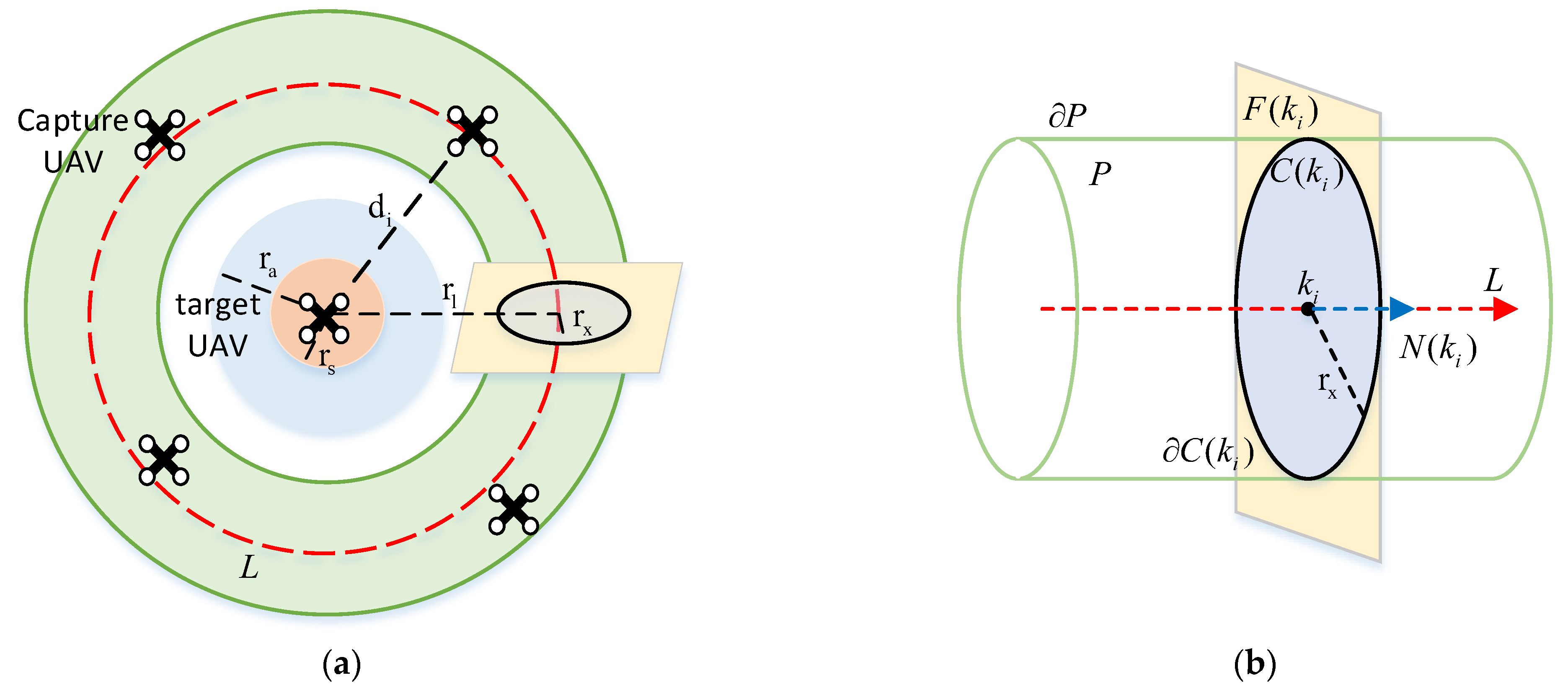
4. Real-Time Dynamic Capture of UAVs Based on Closed Circular Pipeline

In Section 3, a long-distance pursuit–evasion model based on differential game theory is proposed to derive optimal pursuit–evasion strategies for multi-UAV systems in dynamic and uncertain environments. For close-range capture, a closed circular pipeline model is introduced to improve the success rate of UAV capture.

4.1. Capture UAVs Enter the Closed Circular Pipeline

A closed circular pipeline is established to fulfill the requirements of UAV capture missions. Traditional methods typically design a single curve in 3D space to achieve UAV capture. However, the capture mission may require a pipeline rather than a single curve. This configuration allows more UAVs to be accommodated within a single pipeline, thereby better addressing various environmental constraints. Firstly, the predicted position of the target UAV, calculated using the differential game algorithm from the previous section, is employed as the center point for closed circular pipeline construction. Next, the capture UAVs are converged toward the centerline of the closed circular pipeline. During this stage, a shortest-distance-based allocation algorithm is applied to assign capture points to capture UAVs, directing them to approach the target UAV and position themselves around the target UAV in a coordinated manner.

K points are uniformly distributed along the centerline of the closed circular pipeline as capture points; the location of the capture point is shown in Figure 5. A greedy algorithm is employed to select the closest capture point for pre-assignment, followed by the re-assignment of any duplicated capture points based on the matching rule. This method is computationally simple and highly efficient. On the one hand, it ensures that each UAV is evenly distributed around the target UAV, and on the other hand, it minimizes the time difference between each capture UAV’s arrival at the capture point. The flow of the greedy algorithm is shown in Algorithm 1:

Algorithm 1 Greedy Algorithm

The number of capture UAVs in the environment N, the number of capture points k, and the calculation of the position of each capture point $Q_{\mathrm{j}}$.

for i = 1 to N do

for j = 1 to k do

Calculate the distance $D_{\mathrm{ij}}$ from the i-th capture UAV to each capture point $Q_{\mathrm{j}}$

Assign the minimum distance $D_{\mathrm{ij}}$ corresponding to the capture point $Q_{\mathrm{j}}$ to the i-th capture UAV,$Q_{\mathrm{j}}=Q_{\mathrm{j}}+1$

If $Q_{\mathrm{j}}=0$ then

The capture point is not assigned

If $Q_{\mathrm{j}}=1$ then

Upon successful allocation, the pairing of the capture UAV and the capture point is removed from the loop.

Else $Q_{\mathrm{j}}>1$

The capture point is assigned to the capture UAV furthest away, and the paired UAV and capture point are subsequently removed from the loop

end for

end for

4.2. Controller Design of the Capture UAVs After Entering the Closed Circular Pipeline

When the capture UAVs enter the closed circular pipeline based on the greedy algorithm, the velocity command for the i-th capture UAV is formulated as follows:

$${\mathbf{v}}_{\mathrm{i}}=-\mathrm{sat}\left({\mathrm{k}}_1{\mathbf{u}}_{1,i}+{\mathrm{k}}_2{\mathbf{u}}_{2,i}+{\mathrm{k}}_3{\mathbf{u}}_{3,i}+{\mathrm{k}}_4{\mathbf{u}}_{4,i},v_{\max ,i}\right)$$

(16)

where ${\mathrm{k}}_1,{\mathrm{k}}_2,{\mathrm{k}}_3,{\mathrm{k}}_4>0$, $v_{\max ,i}$ > 0, represents the maximum allowable speed of the i-th UAV, and the saturation function is formulated to ensure that $\mathbf{v}$ does not exceed $v_{\max ,i}$.

$$\mathrm{sat}\left({\mathrm{v}}_{\mathrm{i}},{\mathrm{v}}_{\max ,\mathrm{i}}\right)\triangleq \left\{\begin{array}{ll}{\mathrm{v}}_{\mathrm{i}}\hfill & ‖{\mathrm{v}}_{\mathrm{i}}‖\le {\mathrm{v}}_{\max ,\mathrm{i}}\hfill \\ {\mathrm{v}}_{\max ,\mathrm{i}}{\displaystyle \frac{{\mathrm{v}}_{\mathrm{i}}}{\Vert {\mathrm{v}}_{\mathrm{i}}\Vert }}\hfill & ‖{\mathrm{v}}_{\mathrm{i}}‖>{\mathrm{v}}_{\max ,\mathrm{i}}\hfill \end{array}\right.$$

(17)

${\mathbf{u}}_{1,i},{\mathbf{u}}_{2,i},{\mathbf{u}}_{3,i},{\mathbf{u}}_{4,i}$ are subcommands to achieve different purposes. They are shown as follows:

The UAV is directed by ${\mathbf{u}}_{1,i}$ along the positive direction of the closed circular pipeline, ensuring that the capture UAV continuously moves around the target UAV to form a dynamic enclosure.

$${\mathbf{u}}_{1,i}=\mathrm{sat}\left(N\left(x_i\right)v_{\mathrm{e}},v_e\right)$$

(18)

where $v_e$ is the desired speed of the UAV capture.

$u_{2,i}$ is used to enable inter-UAV obstacle avoidance within the closed circular pipeline, preventing potential collision conflicts among UAVs.

$$u_{2,i}={\displaystyle \sum _{j\in {\mathcal{N}}_{\mathrm{m},i}}-}{\sigma }_{\mathrm{m}}\left(‖x_i-x_j‖\right){\displaystyle \frac{x_i-x_j}{‖x_i-x_j‖}}$$

(19)

where ${\mathcal{N}}_{\mathrm{m},i}$ is the neighborhood of the i-th UAV, which is the set of other UAVs that could potentially collide with it. ${\mathrm{r}}_{\mathrm{s}}$ ($r_{\mathrm{a}}>r_{\mathrm{s}}$) is defined as the UAV safety radius, and collision prevention begins when the distance between UAVs exceeds $r_{\mathrm{s}}+r_{\mathrm{a}}$. The function value reaches its maximum when the UAVs distance equals $2r_{\mathrm{s}}$. The objective of the speed command ${\mathbf{u}}_{2,i}$ is to minimize its speed value, ideally approaching zero, which implies that the i-th UAV will not collide with the j-th UAV.

${\sigma }_{\mathrm{m}}(x)\triangleq \sigma \left(x,2r_{\mathrm{s}},r_{\mathrm{s}}+r_{\mathrm{a}}\right)$, the smooth function, is defined as follows:

$$\sigma \left(x,d_1,d_2\right)=\left\{\begin{array}{cc}1& x\le d_1\\ A{x}^3+B{x}^2+Cx+D& d_1\le x\le d_2\\ 0& d_2\le x\end{array}\right.$$

(20)

where $A=-2/{\left(d_1-d_2\right)}^3$, $B=3\left(d_1+d_2\right)/{\left(d_1-d_2\right)}^3$, $C=-6d_1{d}_2/{\left(d_1-d_2\right)}^3$, and $D=d_2^2\left(3d_1-d_2\right)/{\left(d_1-d_2\right)}^3$. This design is suitable for avoiding drastic changes in speed or acceleration near the critical distance, ensuring smoother and more stable flight trajectories for the UAV.

${\mathbf{u}}_{3,i}$ is designed to keep the UAV within the closed circular pipeline, ensuring it does not exceed the pipeline’s boundary.

$${\mathbf{u}}_{3,i}=-{\left(\left({\mathbf{I}}_2-N{\left(x_i\right)}^{\mathrm{T}}N\left(x_i\right)\right){\left({\displaystyle \frac{x_i-x_e}{‖x_i-x_e‖}}\right)}^{\mathrm{T}}\right)}^{\mathrm{T}}{\sigma }_{\mathrm{t}}\left(\left|d_{\mathrm{t},i}\right|\right)$$

(21)

where ${\sigma }_{\mathrm{t}}(x)\triangleq \sigma \left(x,r_{\mathrm{s}},r_{\mathrm{a}}\right)$, and $x_e$ is the center point for the closed circular pipeline. $d_{\mathrm{t},i}$ represents the distance between the UAV and the closed circular pipe wall. No force is applied when the distance exceeds $r_{\mathrm{a}}$; the force begins to act when the distance is less than $r_{\mathrm{a}}$, reaching its maximum when the distance is exactly $r_{\mathrm{s}}$. As the pipe width remains constant, the velocity command is designed to minimize the obstacle avoidance function, ideally reducing it to zero. This ensures that the i-th UAV and its safety zone stay within the closed circular pipe.

${\mathbf{u}}_{4,i}$ controls the uniform capture of the target UAV by the capture UAVs, ensuring an appropriate distance is maintained between each capture UAV.

$$u_{4,i}=\left\{\begin{array}{l}{\displaystyle \sum _{j\in {\mathcal{N}}_{\mathrm{e},i}}}{\sigma }_{\mathrm{e}}\left(\left|l_{ij}\right|\right)N\left(x_i\right),N\left(x_i\right)\cdot (x_i-x_j)>0\\ {\displaystyle \sum _{j\in {\mathcal{N}}_{\mathrm{e},i}}-{\sigma }_{\mathrm{e}}\left(\left|l_{ij}\right|\right)}N\left(x_i\right),N\left(x_i\right)\cdot (x_i-x_j)\le 0\end{array}\right.$$

(22)

where ${\sigma }_{\mathrm{e}}(x)\triangleq \sigma \left(x,2l_{\mathrm{e}},2\alpha l_{\mathrm{e}}\right)$, $\alpha >1$, and $l_{\mathrm{e}}={\displaystyle \frac{L}{2N}}$. To achieve an approximately uniform capture, the circumference of the centerline of the closed circular pipeline is calculated as $L=2\pi r_l$. The relative positions of the two UAVs are represented by the length of the corresponding curve inside the pipeline $l_{\mathrm{ij}}=L{\displaystyle \frac{\theta }{2\pi }}$;$\theta <\pi$ is the angle between the lines connecting two adjacent capture UAVs and the target UAV. When the distance $l_{\mathrm{ij}}$ is greater than $2\alpha l_{\mathrm{e}}$, no force is applied; when the distance is less than $2\alpha l_{\mathrm{e}}$, force starts to be applied; and when the distance equals $2l_{\mathrm{e}}$, the force is maximized. The velocity command ${\mathbf{u}}_{4,i}$ is designed to approach zero or be as small as possible to ensure $l_{ij}=2l_e$. Uniform target capture is achieved when all UAVs satisfy these conditions.

The designed controller integrates multiple subcommands to achieve several key objectives: it forms a dynamic and stable distribution around the target UAV, prevents inter-UAV collisions through robust obstacle avoidance mechanisms, and maintains confinement within the pipeline boundary to ensure structural stability. Additionally, it ensures a uniform distribution of UAVs for optimal capture efficiency and guarantees smooth and stable UAV trajectories, thereby enhancing both safety and reliability.

4.3. Stability Analysis

To ensure the stability of the controller, we adopt a mathematical approach based on Lyapunov’s stability theory. A Lyapunov function is defined as follows:

$$V=V_1+V_2+V_3+V_4$$

(23)

where $V_1={\displaystyle \frac{1}{2}}{{\displaystyle \sum _{\mathrm{i}=1}^N‖v_i-v_{\mathrm{e}}‖}}^2$, $V_2={\displaystyle \frac{1}{2}}{\displaystyle \sum _{i,j\in {\mathcal{N}}_i}{\sigma }_{\mathrm{m}}\left(‖x_i-x_j‖\right)}$, $V_3={\displaystyle \frac{1}{2}}{\displaystyle \sum _{i=1}^N{\sigma }_{\mathrm{t}}\left(\left|d_{\mathrm{t},i}\right|\right)}$, and $V_4={\displaystyle \frac{1}{2}}{\displaystyle \sum _{i=1}^N{\displaystyle \sum _{j=1,j\ne i}^N{\sigma }_{\mathrm{e}}\left(\left|l_{ij}\right|\right)}}$. By using the velocity command (16) for all UAVs, $\stackrel{•}{V}$ satisfies $\stackrel{•}{V}\le 0$, and the system is stable.

5. Results

5.1. Test Platforms

In this study, the Rflysim platform was utilized for both simulation and real flight testing [25,26]. The platform adopts a model-based (MBD) design concept, which integrates Pixhawk/PX4, MATLAB/Simulink, and ROS, along with commercial off-the-shelf (COTS) smart hardware. It enables simulation and real-time flight/motion testing for unmanned intelligent body control, clustering, and vision-based operations. To address the aforementioned issues, unmanned system modeling, controller design, software-in-the-loop (SIL) simulation, and hardware-in-the-loop (HIL) simulation were performed. MATLAB.

Simulink’s automatic code generation feature allowed for convenient and automatic controller deployment to the hardware, facilitating HIL simulation and real flight testing to achieve Sim2Real. Figure 6 shows the connection mode of the hardware device.

5.2. Scenario Design

In this section, a typical scenario is constructed involving four capture UAVs and one target UAV. The numerical simulation was conducted on a computer running Matlab 2023b, with a simulation time step of 0.03 s. The simulation utilized the following parameters and initial conditions: the wheelbase of each UAV is 150 mm, the obstacle avoidance radius is 0.6 m, the maximum speed is 5 m/s, and the predefined closed circular pipeline radius is 0.5 m. The simulation began with all UAVs randomly positioned in 3D space and an initial speed of zero.

Figure 7 shows the simulation results of four capture UAVs rounding up a target UAV. The simulation results indicate that, within a certain time frame, both the capture UAVs and the target UAV follow the directions prescribed by the differential game calculation without deviation. This strategy is optimal for both pursuit and evader. Once the distance between the capture UAVs and the target UAV is less than the capture radius, the capture UAVs initiate the capture. Ultimately, the capture UAVs successfully complete the capture task.

5.3. Analysis of Experimental Results

The simulation results are analyzed through the capture success rate, the capture time, and the total length of the path; the simulation experiment results are shown in

Table 2. Simulation experiment results.

Indicator Name	This Paper	Flux Guidance	Least Squares
Capture Success Rate	93%	89%	78%
Capture Time(s)	18.7	23.8	31.9
The total length of the path	12.4	17.8	23.3

.

Using five quadcopter UAVs to form the above-mentioned typical scenario, the motion capture system provides real-time positional information of the quadcopter UAVs during actual flights.

The Rflysim platform transfers the real-time states of these UAVs into the Rflysim simulation environment through the virtual-reality interface of the centralized control base station, thereby achieving integration of simulation and real flight data and completing the mapping and reverse mapping for a combination of virtual and real environments. In the actual flight photos, the capture UAVs are marked with red circles, and the target UAV is marked with a blue circle.

The experiment has a duration of 30 s, with six representative snapshots presented in Figure 8. Figure 8a illustrates the initial positions of each UAV. At t = 0 s, the UAVs take off and initiate target search, as shown in Figure 8b. At t = 8 s, the capture UAVs monitor and rapidly track the target UAV using a differential game algorithm, as illustrated in Figure 8c. At t = 12 s, the distance between the capture UAVs and the target UAV falls below the capture radius, initiating the convergence of the four UAVs around the target. The closer UAVs autonomously position themselves within the closed circular pipeline, awaiting the remaining capture UAVs to complete their positioning, as shown in Figure 8d. At t = 15 s, the four capture UAVs approach the target following the predefined capture path, as shown in Figure 8e. At t = 18.7 s, the four capture UAVs complete the uniform capture of the target UAV, as illustrated in Figure 8f.

The first through fourth UAVs serve as the capture UAVs, while the fifth UAV functions as the target UAV. Figure 9 illustrates the distance between the capture UAVs and the target UAV during the capture process. Until 8.5 s, the target UAV moved forward to evade the capture UAVs. From 8.5 to 18.7 s, the target UAV was actively tracked, initiating the capture once the distance between the capture UAVs and the target UAV was less than the capture radius. After 18.7 s, the capture UAVs maintain continuous and uniform capture of the target UAV.

Taking the distance between the fifth target UAV and the first capture UAV as an example, Figure 10 illustrates the three phases of UAV capture: initially, from 0 to 8.5 s, the target UAV moves forward to evade, while the capture UAV hovers, resulting in an increase in the distance between them. Next, from 8.5 to 18.7 s, the target UAV continues its evasion, while the capture UAVs initiates tracking and begins to capture the target UAV. Finally, after 18.7 s, the capture UAV establishes continuous capture and maintains uniform capturing of the target UAV, keeping the distance between the two UAVs consistently below 2 m, which is the sum of the capture radius and the closed circular pipeline radius.

6. Conclusions

In this paper, a real-time dynamic multi-UAV capture strategy based on the differential game model is proposed to address the challenge of capturing target UAVs. The optimal strategy for attaining the Nash equilibrium through differential games enables the capture UAVs to effectively track the target UAV. Additionally, this paper introduces a collaborative multi-UAV target capture approach using closed circular pipeline control. This method ensures that the capture UAVs are evenly distributed around the target UAV, which facilitates the smooth capture process. By constraining the capture UAVs within the closed circular pipeline, clustering and overcrowding are prevented, thereby enhancing the efficiency and effectiveness of the capture operation. Research and experimentation demonstrate the effectiveness of the proposed strategies and methods in successfully capturing the target UAV. The combination of the differential game model and closed circular pipeline control facilitates the coordination and distribution of capturing UAVs, thereby enhancing the success rate of UAV formation capture.

In future research, efforts will focus on further extending and optimizing the existing multi-UAV real-time dynamic capture and collaborative methods. By accounting for adversarial occupancy uncertainty and resource availability, the applicability and robustness of the method can be enhanced, ensuring its effectiveness in dynamic environments.

UAV maneuver decision-making algorithms will be implemented to enhance UAV efficiency during operation, particularly for path planning in unknown and dynamic environments. These future efforts are expected to further enhance the practical applicability of multi-UAV cooperative strategies, providing robust theoretical and technical support for UAV technology in complex missions.