Article

A New Hybrid Improved Kepler Optimization Algorithm Based on Multi-Strategy Fusion and Its Applications

1
School of Information Science and Technology, Yunnan Normal University, Kunming 650500, China
2
Southwest United Graduate School, Kunming 650092, China
*
Author to whom correspondence should be addressed.
Mathematics 2025, 13(3), 405; https://doi.org/10.3390/math13030405
Submission received: 1 January 2025 / Revised: 15 January 2025 / Accepted: 19 January 2025 / Published: 26 January 2025
(This article belongs to the Special Issue Metaheuristic Algorithms, 2nd Edition)

Abstract

:
The Kepler optimization algorithm (KOA) is a metaheuristic algorithm based on Kepler’s laws of planetary motion and has demonstrated outstanding performance in multiple test sets and for various optimization issues. However, the KOA is hampered by the limitations of insufficient convergence accuracy, weak global search ability, and slow convergence speed. To address these deficiencies, this paper presents a multi-strategy fusion Kepler optimization algorithm (MKOA). Firstly, the algorithm initializes the population using Good Point Set, enhancing population diversity. Secondly, Dynamic Opposition-Based Learning is applied for population individuals to further improve its global exploration effectiveness. Furthermore, we introduce the Normal Cloud Model to perturb the best solution, improving its convergence rate and accuracy. Finally, a new position-update strategy is introduced to balance local and global search, helping KOA escape local optima. To test the performance of the MKOA, we uses the CEC2017 and CEC2019 test suites for testing. The data indicate that the MKOA has more advantages than other algorithms in terms of practicality and effectiveness. Aiming at the engineering issue, this study selected three classic engineering cases. The results reveal that the MKOA demonstrates strong applicability in engineering practice.

1. Introduction

With the rapid advancement of technology and the increasing complexity of engineering practice, the scale and complexity of optimization challenges are progressively escalating. These practical optimization issues typically feature multimodality and high dimensionality, accompanied by a multitude of local optima and tight, highly nonlinear constraints, such as feature selection [1], image processing [2], wireless sensor networks [3], UAV route planning [4], and job shop scheduling problems [5]. Conventional optimization techniques, including the gradient descent, Newton method, and conjugate gradient algorithms, typically solve problems by constructing precise mathematical models. These classical algorithms are computationally inefficient and computationally intensive, making it a powerless choice to utilize traditional approaches to address optimization issues [6]. Metaheuristic algorithms (MAs) are widely regarded as a common approach to solve optimization issues because of their flexibility, practicality, and robustness [7].
MAs are divided into four categories: evolutionary algorithms (EAs), swarm intelligence algorithms (SIAs), optimization algorithms derived from human life activities, and optimization algorithms based on physical law [8]. The categorization of MAs is presented in Figure 1.
Natural evolution processes inspire the design of the EAs. The genetic algorithm (GA) [9] is among the most famous and classic evolutionary algorithms, and its variants are continuously studied and proposed [10,11]. GAs are founded on Darwin’s theory of natural selection, where the optimal population is arrived at through iterative processes involving selection, crossover, and mutation. This category of algorithms is also extensive in scope; The coronavirus optimization algorithm (COA) [12] models the spread of the coronavirus starting from patient zero, taking into account the probability of reinfection and the implementation of social measures. In addition, differential evolutionary algorithms (DEs) [13], the invasive tumor growth optimization algorithm (ITGO) [14], the love evolution algorithm (LEA) [15], and so on belong to the category of EAs.
The SIAs are primarily inspired by the behaviors of biological groups, applying the characteristics of certain animals in nature, such as their survival strategies and behavioral patterns, to the development of these algorithms. An example is particle swarm optimization (PSO), which draws inspiration from the predatory behavior of birds [16]. In a standard PSO algorithm, one updates the particle’s position using both the globally optimal particle’s position and its own optimal (local) position. The movement of the entire swarm transitions from a disordered state to an ordered one, ultimately converging with all particles clustering at the optimal position. Dorigo introduced the ant colony optimization (ACO) algorithm in 1992, which draws inspiration from how ants forage [17]. The ACO algorithm mimics the process in which ants leave pheromone trails while foraging, guiding other ants in selecting their paths. In this process, the shortest route was determined according to greatest pheromone concentration. The SIAs also include the gray wolf algorithm (GWO) [18], Harris hawk algorithm (HHO) [19], whale optimization algorithm (WOA) [20], sparrow search algorithm (SSA) [21], sea-horse optimizer (SHO) [22], seagull optimization algorithm (SOA) [23], dung beetle optimizer (DBO) [24], nutcracker optimizer algorithm (NOA) [25], and marine predators algorithm (MPA) [26].
The third kind of metaheuristics is optimization algorithms based on human life activities, which is inspired by human production processes and daily life. Teaching–Learning-Based Optimization (TLBO) [27] is the most well-known algorithm of this type. The TLBO simulates the conventional process of teaching. The entire optimization process encompasses two stages. During the teacher stage, each student studies from the best individual. At the learner stage, each student absorbs knowledge from their peers in a random process. The inspiration for the political algorithm (PO) [28] comes from people’s political behavior. The volleyball premier league algorithm (VPLA) [29] simulates the interaction and the dynamic competition between diverse volleyball teams. The queuing search algorithm (QSA) [30] draws inspiration from human queuing activities.
As the last type of MAs, optimization algorithms grounded in physical laws are inspired by algorithms abstracted from mathematics and physics. For instance, simulated annealing (SA) [31], the energy valley optimizer (EVO) [32], the light spectrum optimizer (LSO) [33], the gravitational search algorithm (GSA) [34], central force optimization (CFO) [35], and the sine–cosine algorithm (SCA) [36] belong to this category.
Among the many MAs available, the Kepler optimization algorithm (KOA) [37] is an optimization algorithm grounded in physical laws. The test results of KOA in multiple test sets demonstrate that it is an effective algorithm for dealing with many optimization problems, proving its superior performance. The KOA shows outstanding performance thanks to several key mechanisms: it uses the planetary orbital velocity adjustment mechanism to achieve a balance among exploration and exploitation, simulates the characteristics of the orbital motion of planets in the solar system by dynamically adjusting the search direction to avoid local optimal, and adopts an elite mechanism to ensure that the planets and the sun reach the most favorable position. Currently, the KOA has been utilized to address many practical issues in real life. Hakmi and his team [38] adopted the KOA to address the combined heat and power units’ economic dispatch in power systems. Houssein et al. [39] developed an improved KOA (I-KOA) and applied it to feature selection in liver disease classification. In the field of CXR image segmentation at different threshold levels, Abdel Basset and colleagues [40] used the KOA for optimization. In addition, the KOA has also been applied in the field of photovoltaic research [41,42]. After a comprehensive review and comparative analysis of the relevant academic literature, apparently, the KOA shows exceptional performance and competitiveness in addressing complex optimization issues.
However, according to the No Free Lunch (NFL) theorem [43], no single MA can effectively address every optimization issue. This motivates us to continuously innovate and refine existing metaheuristic algorithms to address diverse problems. Therefore, the KOA has been undergoing continuous improvements since its introduction, with the aim of maximizing its capability to solve various engineering application problems. Regarding the shortcomings of theKOA, this paper continues to explore new improvement strategies based on previous work and introduces a multi-strategy fusion KOA algorithm (MKOA).

1.1. Paper Contributions

The summary is listed below:
A multi-strategy fusion Kepler optimization algorithm (MKOA) is proposed.
In the testing of CEC2017 and CEC2019, the proposed MKOA is validated to be better than comparison algorithms.
Three real-world engineering optimization challenges are addressed using the proposed algorithm, which highlights the advantages of the algorithm in engineering practice.

1.2. Paper Structure

The layout is outlined below. In Section 2, the principles of the KOA are introduced. In Section 3, the MKOA is proposed, and four improved strategies are introduced. The statistical results of the MKOA in CEC2017 and CEC2019 are presented in Section 4. The implementation of the MKOA in three practical engineering optimization scenarios is discussed in Section 5. Finally, the last chapter gives a summary.

2. Principle of Kepler Optimization Algorithm

Abdel Basset et al., drawing inspiration from the laws of celestial motion, proposed the KOA [37]. This algorithm is specifically designed to address single objective optimization issues and continuous optimization issues. Its core mechanism simulates the elliptical orbit motion of planets around the sun, efficiently searching to find the best solution. The KOA has powerful global optimization capability and high solving precision when dealing with these problems. We will elaborate on the mathematical model of the KOA in detail next.

2.1. Initialization

During the initialization process, the KOA initializes N planets randomly in the entire solution domain, each with d dimensions. Its mathematical model is given by
X i j = X i , l b j + r × X i , u b j X i , l b j , i = 1 , 2 , , N j = 1 , 2 , , d
where X i j are the position of the i t h planet in the j t h dimension; X i , l b j and X i , u b j denote the minimum and maximum bounds of the j t h dimension. r represents a randomly selected number with a value between 0 and 1; in addition, the KOA also needs to initialize the orbital eccentricity e using Equation (2), as well as orbital period T through Equation (3).
e i = r , i = 1 , 2 , , N
T i = | r n | , i = 1 , 2 , , N
where r n represents a value which is the result of a random sample from a Gaussian distribution.

2.2. Defining the Gravitational Force (F)

The gravity between the planet and the star affects the planet’s orbital velocity. Specifically, the orbital velocity of the planet exhibits a pattern: it increases when the planet approaches the star; otherwise, the orbital velocity decreases. The gravitational model is shown below:
F g i t = e i × μ t × M ¯ s × m ¯ i R ¯ 2 i + λ + r 1
where e i is the eccentricity, and  μ denotes the universal gravitational parameter; r 1 is a randomly selected value among [0, 1]; λ is a constant value; M s and m i denote the mass of the sun and the planet, respectively, and the mathematical representations are given by Equations (7) and (8). M ¯ s and m ¯ i denote their respective normalized forms. R ¯ i represents the normalized value of the Euclidean distance R i among the sun X s and the planet X i . The  R i is given here:
R i t = X s t X i t 2 = j = 1 d X S , j ( t ) X i , j ( t ) 2
R ¯ i = R i t min ( R ( t ) ) max ( R t ) min ( R ( t ) )
M s = f i t s t w o r s t ( t ) k = 1 N ( f i t k t w o r s t ( t ) )
m i = r 2 f i t i t w o r s t ( t ) k = 1 N ( f i t k t w o r s t ( t ) )
where
f i t s t = b e s t t = k 1 , 2 , , N m i n f i t k ( t )
w o r s t t = k 1 , 2 , , N m a x f i t k ( t )
where r 2 represents a randomly selected value among [0, 1]. The mathematical model of μ t is given below:
μ t = μ 0 × exp ( γ t T m a x )
where μ 0 and γ are predefined values; in addition, t is the current number of cycles, and the maximum cycle count is T m a x .

2.3. Calculating an Object’s Velocity

The orbital velocity increases when the planet approaches the star; otherwise, the orbital velocity decreases. When an object approaches the star, the gravity becomes exceedingly potent. As a result, each planet attempts to accelerate in order to resist the intense gravity of the star. The description of the mathematical model is provided below:
v i t = δ × 2 r 4 × X i X b + δ ¨ × X a X b + 1 R i n o r m ( t ) × σ × U 1 × r 5 × X i , u b X i , l b , i f R i n o r m ( t ) 0.5 r 4 × κ × X a X i + 1 R i n o r m ( t ) × σ × U 2 × r 5 × r 3 × X i , u b X i , l b , e l s e
δ = U × M × κ , δ ¨ = 1 U × M × κ
κ = μ t × m i + M s × 2 R i ( t ) + ε 1 a i ( t ) + ε 1 2
M = r 3 × 1 r 4 + r 4 , M = r 3 × 1 r 5 + r 5
U = 0 , i f r 5 r 6 1 , e l s e
σ = 1 , i f r 4 0.5 1 , e l s e
U 1 = 0 , i f r 5 r 4 1 , e l s e , U 2 = 0 , i f r 3 r 4 1 , e l s e
where v i ( t ) is the i t h planet’s speed; r 3 and r 4 are probabilistic variables with a uniform distribution over the interval 0 to 1; r 5 and r 6 are two binary vectors, each component of which can only be 0 or 1; X a and X b denote planets that are randomly chosen from the current solutions; and σ is a number that is randomly chosen to be either −1 or 1 within the band for adjusting the exploration direction. a i ( t ) is the semi-major axis of the elliptical orbit for object i at time t. The following is the formula used to compute a i ( t ) :
a i t = r 3 × T i 2 × μ t × ( M s + m i ) 4 π 2 1 3

2.4. Escaping from Local Optimum

Most planets revolve counter-clockwise near the star. However, some planets deviate from this norm by orbiting in the reverse direction. In original KOA, this behavior is leveraged to modify the exploration direction, helping the KOA escape local optima. The algorithm introduces a control variable, σ , which dynamically modifies the direction of the search, thereby controlling the orbit direction of a planet around the star. This approach increases the likelihood that agents will effectively explore the entire search space.

2.5. Updating Objects’ Positions

Planet follow Kepler’s law and orbit the sun periodically along their respective elliptical trajectory. Planets rotate near the sun. Over time, they first approach the star and then gradually move further away. The KOA elaborates on this behavior through two key steps: exploration and exploitation. In the KOA, exploration operations are carried out when planets are located further away from the star; when the planet approaches the star, exploitation operations are carried out. Its mathematical model is given by
X i t + 1 = X i t + σ × V i t + U × ( F g i t + r ) × X S t X i t

2.6. Updating the Distance from the Sun

To enhance the KOA’s search ability, the KOA simulates the fluctuating normal distance behavior between planets and the sun over time. When the planet is located near the star, the exploitation operator is activated to enhance the convergence rate of the algorithm; on the other hand, when the planet is located further away from the star, the exploration operator is activated to escape local optima. To apply the idea to the KOA, we introduce the control parameter h, which varies with the number of runs. When control parameter h is greater, the solution space is expanded by using detection operators to explore better solutions; otherwise, it focuses on the area surrounding the current optimal individual to maximize the benefits. This is expressed mathematically as Equation (21):
X i t + 1 = X i t × U 1 + 1 U 1 × X i t + X s t + X a t 3 + h × X i t + X s t + X a t 3 X b t
h = 1 e η r
where r represents a randomly selected value among [0, 1]; the variable η denotes a linear diminishing factor between 1 and −2, while η has the following definition:
η = a 2 1 × r 4 + 1
where a 2 represents the cyclic control parameter, as detailed in Equation (24) below.
a 2 = 1 t % T m a x T C T m a x T C
where T C is a constant value, and % represents the remainder operation.

2.7. Elitism Mechanism

At this stage, we implemented an elite mechanism to assure that the star as well as the planets reach their most favorable positions. Equation (25) provides a summary of this strategy.
X i t + 1 = X i t + 1 , i f f X i t + 1 f X i t X i t , e l s e

2.8. KOA Pseudocode

Algorithm 1 presents the KOA’s complete pseudocode.
Algorithm 1 KOA Pseudocode
Input:  N, T m a x , μ , γ , T ¯
1:Initialization
2:Evaluation
3:Identify the current best solution X s
4:while t < T m a x  do
5:   Update e i , μ t , b e s t t , as well as w o r s t t
6:   for  i = 1 : N  do
7:     Calculate R ¯ i using Equation (6)
8:     Calculate F g i using Equation (4)
9:     Calculate v i using Equation (12)
10:     Generates two independent random variables, denoted as r and r 1
11:     if r > r 1  then
12:        Use Equation (20) to update planets’ positions
13:     else
14:        Use Equation (21) to update planets’ positions
15:     end if
16:     Apply an elitist mechanism to select the optimal position, using Equation (25)
17:   end for
18:   t = t + 1;
19:end while
Output:  X s

3. The Proposed Multi-Strategy Fusion Kepler Optimization Algorithm (MKOA)

Resembling other metaheuristic algorithms, the KOA also faces challenges such as premature convergence as well as a weak global search ability, especially when addressing high-dimensional and complicated issues [44]. Therefore, to improve these defects of the KOA, this article integrates the Good Point Set strategy, the Dynamic Opposition-Based Learning strategy, the Normal Cloud Model strategy, and the New Exploration strategy to amplify the original KOA. The strategies proposed will be discussed thoroughly in the following sections in this part.

3.1. Good Point Set Strategy

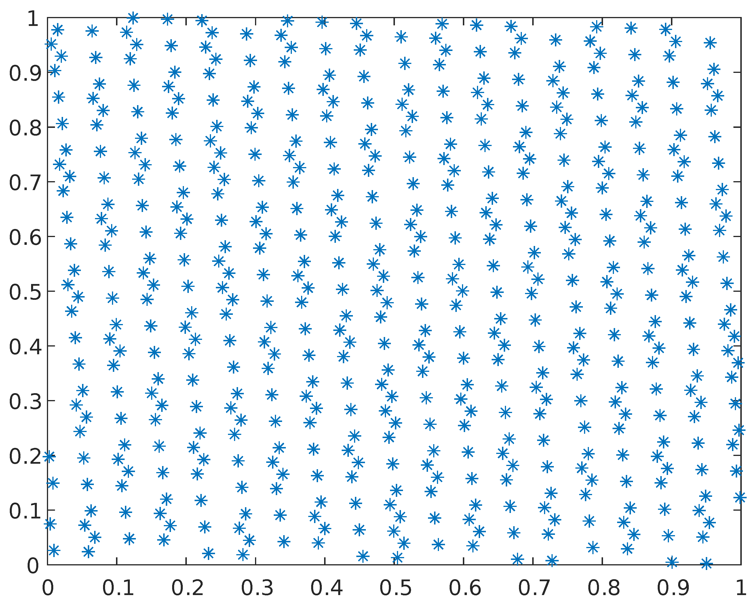
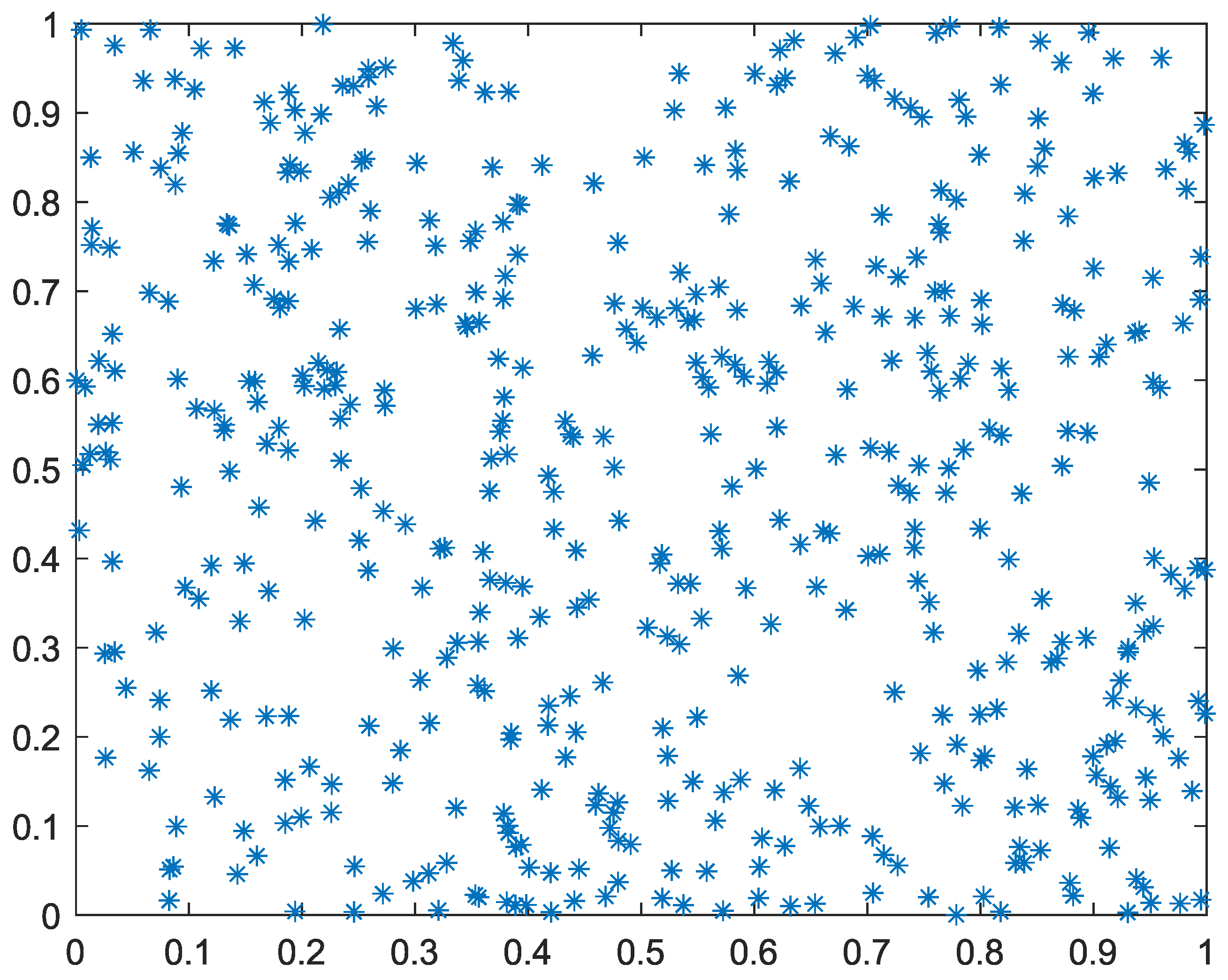
In MAs, the algorithm’s global search ability is influenced by the location of the initial population. The traditional Kepler optimization algorithm (KOA) utilizes the random method for population initialization, which leads to drawbacks such as uneven population distribution. This paper introduces a Good Point Set (GPS) strategy to improve the KOA by ensuring the initial solution is evenly distributed across the search domain.
The concept of GPS was introduced by Hua and Wang in 1978 [45]. This strategy enables the search space to be as uniformly covered as possible, even with a relatively small number of sample points [46]. Therefore, it has been used by many scholars in population initialization.
The basic definition of the GPS strategy is as given below: Define G s as a standard cube with side length one in an s-dimensional Euclidean space. If  r G s , which may be represented as
p n k = r 1 ( n ) k , r 2 ( n ) k , , r s ( n ) k , 1 k n
φ n = C r , ε n 1 + ε
where p n k is the point set, as well as if p n k deviation satisfies Equation (27), it is called Good Point Set. C r , ε n 1 + ε is a fixed value that is only related to ε and r; r s ( n ) k denotes the decimal fraction of the value; n denotes the sample size; and r is computed as follows:
r = 2 × c o s 2 π k p k = 1 , 2 , , n
where p is the smallest prime that satisfies s p 3 / 2 .
The GPS strategy is applied to population initialization. The initialization equation of the i t h individual is given by
X i j = X i , l b j + r j ( i ) k × X i , u b j X i , l b j , i = 1 , 2 , , N j = 1 , 2 , , d
Figure 2 and Figure 3, respectively, show the comparison between the two-dimensional point sets generated by the GPS method and the random method when the population size is 500. Figure 4 illustrates a frequency distribution histogram of the initialized population using the two methods. As shown in the figure, the GPS strategy is more uniform than the randomly generated strategy. In addition, when the sample size is consistent, the distribution of the GPS strategy is similarly consistent, which means that the GPS strategy is stable.

3.2. Dynamic Opposition-Based Learning Strategy

Tizhoosh [47] came up with Opposition-Based Learning (OBL) in 2005, drawing inspiration from the idea of opposition. Until now, the OBL strategy and its enhancements have been widely applied in various optimization algorithms [48,49,50]. The OBL strategy has the following definition:
X ^ i = L B + U B X i
where X i and X ^ i are the original solution and the opposite solution, respectively; the symbols L B and U B represent the lower as well as the upper limit of the search domain.
Between the initial solution and the reverse solution, the OBL strategy will select the solution with a higher fitness value for the next population iteration. Although it can effectively improve the diversity as well as the quality of the population, the constant distance maintained between the original solution and the generated opposite solution results in a lack of certain randomness. Therefore, it may hinder the optimization of the algorithm throughout the entire iteration process. To address the shortcoming of the OBL strategy, this study proposes a Dynamic Opposition-Based Learning (DOBL) strategy to further improve the diversity as well as the quality of the population.
The DOBL strategy [49] introduces a dynamic boundary mechanism grounded in the original OBL strategy, thereby improving the problem of insufficient randomness in the original OBL strategy. The mathematical model of DOBL strategy is given by
X ^ i , j t = a j t + b j t X i , j t
where X ^ i , j t and X i , j t , respectively, represent the reverse solution and the original solution for the j-th dimension of the i-th vector during the t-th iteration; a j t and b j t , respectively, represent the lower and upper values in the j-th dimension during the t-th iteration. The mathematical models of a j t and b j t are shown as
a j t = m i n X j t , b j t = m a x X j t
The KOA’s search phase is altered using the DOBL strategy to boost the diversity as well as the quality of the population. In the KOA, the DOBL strategy simultaneously considers the original solution and reverse solution. Sorting according to fitness values, we will select only the top N optimal solutions. Algorithm 2 presents the pseudocode of DOBL.
Algorithm 2 DOBL strategy Pseudocode
Input: D, N, X // D: dimensionality; N: population size; X: original solutions
1:for  i = 1 : N   do
2:   for  j = 1 : D  do
3:      X ^ i , j t = a j t + b j t X i , j t // Generate opposite solution through Equation (31)
4:   end for
5:end for
6:Evaluate population fitness values (Including the original solution as well as the opposite solution)
7: X Select N best individuals from set { X , X ^ }
Output: X

3.3. Normal Cloud Model Strategy

In evaluating the significance of the current best individual position, we found that in the KOA, the information utilization of the optimal solution is not sufficient, which often makes the KOA prone to local optima. Thus, this study introduces a Normal Cloud Model (NCM) strategy [51] to perturb the current best solution. The principle is to perturb the optimal individual by utilizing the randomness and fuzziness of the NCM strategy to extend the search space of the KOA. Its definitions are given below.
Suppose X is a quantitative domain, and that F is a qualitative notion defined over X. x is an element of X and x represents a random instantiation of notion F. μ F x ϵ 0 , 1 is the degree of certainty of x with respect to F. μ : X [ 0 , 1 ] , x X , x μ x . So, x is referred to as a cloud droplet, and the distribution of x on the entire quantitative domain X is called a cloud. In order to reflect the uncertainty of the cloud, we use three parameters to explain it: expectation, E x ; entropy, E n ; and hyper-entropy, H e . The explicit explanations are detailed below:
(1)
E x represents the anticipated distribution of a cloud droplet.
(2)
E n denotes the uncertainty of cloud drop, and reflects the range of distribution and the spread of the cloud droplet.
(3)
H e is the uncertainty quantification of entropy, which describes cloud thickness and reflects the degree to which the qualitative concept deviates from a normal distribution.
If x satisfies x N E x , E n 2 , where E n 2 = N E n , H e 2 , and E n 0 , the degree of certainty y for the qualitative variable x is calculated as follows:
y = e ( x E x ) 2 2 E n 2
At this point, the distribution of x over the entire quantitative domain X is called a normal cloud. y denotes the anticipated curve for the NCM strategy. Figure 5 illustrates images of normal clouds with different parameter features. From Figure 5a,b, it is possible to observe that with the increase in H e , the dispersion of cloud droplets also simultaneously increases; from Figure 5a,c, it is possible to observe that as E n increases, the distribution range of cloud droplets also expands. Therefore, Figure 5 indirectly reveals the fuzziness as well as the randomness characteristics of cloud droplets.
The process of converting qualitative concepts to quantitative representations is called a forward normal cloud generator (NCG). By setting appropriate parameters, the NCG generates cloud droplets that fundamentally follow a normal distribution. The process of cloud droplet generation by means of a cloud generator is outlined below:
x = N C G E x , E n , H e , N c
In Equation (34), N c represents the anticipated number of cloud droplets. Introducing the above NCM into the KOA perturbs the optimal individual. The NCG mathematical model is represented by Equation (35):
x ^ b e s t t = N C G x b e s t t , E n , H e , D
where x b e s t t is the optimal solution of the population during the t-th iteration, and D refers to the dimension of the optimal individual.

3.4. New Exploration Strategy

We apply a new location-update strategy to the original KOA. This strategy effectively balances local and global exploration by integrating the current solution, optimal solution, and suboptimal solution, thereby improving the convergence accuracy as well as maintaining its convergence speed.
The modified Equations (12) and (21) are described by Equations (36) and (37), respectively.
v i t = δ × 2 r 4 × X i X m + δ ¨ × X m X b + 1 R i n o r m ( t ) × σ × U 1 × r 5 × X i , u b X i , l b , i f R i n o r m ( t ) 0.5 r 4 × κ × X m X i + 1 R i n o r m ( t ) × σ × U 2 × r 5 × r 3 × X i , u b X i , l b , e l s e
X i t + 1 = X i t × U 1 + 1 U 1 × X m + h × X m X b t
where X m is defined as follows:
X m = X c s + X o s + X s s 3
where X c s represents the current solution; X o s denotes the optimal solution; and X s s represents the suboptimal solution.

3.5. The MKOA Implementation Process

The MKOA first initializes the population using Good Point Set, enhancing population diversity and introducing a new OBL strategy, “Dynamic Opposition-Based Learning”, to enhance its global exploration ability. Additionally, the NCM method is utilized for the current best solution, introducing perturbation and mutation to enhance local escape capability. Finally, the KOA uses a new position-update strategy to enhance solution quality. All in all, Algorithm 3 presents the pseudocode of the MKOA, and the flow chart of the MKOA appears in Figure 6.
Algorithm 3 Pseudocode of the MKOA
Input: N, T m a x , μ , γ , T ¯
1:Initialization the population by introducing Good Point Set through Equation (29)
2:Evaluation fitness values for initial population
3:Identify the current best solution X s
4:while t < T m a x  do
5:   Update e i , μ t , b e s t t , and  w o r s t t
6:   Update the population location using DOBL strategy by Equation (31)
7:   for  i = 1 : N  do
8:     Calculate R ¯ i using Equation (6)
9:     Calculate F g i using Equation (4)
10:     Calculate v i using Equation (36)
11:     Generates two independent random variables, denoted as r and r 1
12:     if r > r 1  then
13:        Use Equation (20) to update planets’ positions
14:     else
15:        Use Equation (37) to update planets’ positions
16:     end if
17:     Apply an elitist mechanism to select the optimal position, using Equation (25)
18:   end for
19:   Evaluation fitness values and determine the best solution X s
20:   Disturb X s using the NCM strategy by Equation (35)
21:   t = t + 1;
22:end while
Output:  X s

4. Experiments and Discussion

In this part, we evaluate the MKOA’s performance on a range of test suites and conduct experiments to analyze the effect of improvement strategies. In addition, the Wilcoxon rank-sum test was used for an analysis of differences among competitors and overall performance.

4.1. Experimental Environment

The MKOA was implemented using Matlab 2022a version. The simulation experiment environment was as follows: 64-bit Windows10 operating system, AMD Ryzen 5 5600 CPU @ 3.50 GHz, 16.00 GB memory.

4.2. Competitor Algorithms

To test the performance of the MKOA, the MKOA and comparison algorithms were tested by CEC2017 test suite and CEC2019 test suite. We compared the MKOA’s performance to eight other popular optimization algorithms, including the Kepler optimization algorithm (KOA) [37], the Harris hawk algorithm (HHO) [19], the dung beetle optimizer (DBO) [24], the whale optimization algorithm (WOA) [20], the gray wolf algorithm (GWO) [18], the sparrow search algorithm (SSA) [21], the giant trevally optimizer (GTO) [52], and the velocity pausing particle swarm optimization (VPPSO) [53]. Table 1 gives default settings information for these competing algorithms; N and T m a x are fixed at 30 and 500, respectively. These algorithms incorporate diverse advanced search techniques and structures. Most of them offer significant advantages and have been recommended in recent years. Comparing the proposed algorithm with eight other algorithms highlights its superiority in addressing similar problems, demonstrating its effectiveness and potential to enhance future research efforts.

4.3. CEC2017 Test Suite Experimental Results

To assess the optimization effectiveness of the MKOA, we selected the CEC2017 test function, a complex benchmark function for testing optimization algorithms [54]. CEC2017 includes 29 test functions. It consists of four types: Unimodal (F1 and F3), multimodal (F4–F10), hybrid (F11–F20), and composite (F21–F30). In addition, because of the instability of the F2 function, it was removed from the set. Therefore, we did not conduct experiments on F2. F1–F10 functions were utilized to analyze the MKOA’s optimization ability, while the more complicated F11–F30 functions were applied to assess the MKOA’s capability to escape local optimum.

4.3.1. CEC2017 Statistical Results Analysis

This section utilizes CEC2017 to assess the algorithm’s performance, maintaining a dimension fixed at 30. To assure the effectiveness of the experiment, all algorithms were carried out twenty times independently. Table 2 presents the experimental results. Performance metrics include best value, average value, and standard deviation. Bold represents the optimal result.
Through the analysis of Table 2, it can be found that among the 29 functions, the MKOA successfully obtained 22 best solutions, accounting for 75.8%. For F1–F9 test functions, the MKOA obtained the best average fitness value among five test functions (F3–F4, F6–F7, F9). Regarding F1, F5, and F8, the MKOA performed better than the original KOA. In addition, for hybrid and composite functions F10–F30, the MKOA ranks first in the average count of optimal solutions (F11–F20, F22–F25, F27, F29–F30), and it also showed strong competitiveness in most of the other function tests. In summary, the MKOA demonstrates strong capability to handle complicated issues and has better robustness.

4.3.2. Analysis of CEC2017 Convergence Curve

Figure 7 presents the convergence curves of the MKOA, KOA, HHO, DBO, WOA, GWO, SSA, GTO, and VPPSO for the CEC2017 test set in a 30-dimensional setting. The specific analysis is given below:
For the simple peak function F1, the MKOA is similar to the SSA with respect to convergence accuracy and rate. For the simple peak function F3, the MKOA shows a comparable convergence speed to the other algorithms. However, over time, the MKOA achieves a superior solution.
For the simple multimodal problems, F4–F7 and F9, the MKOA’s superior exploration capabilities enable it to converge more quickly and reach better positions. For the multimodal problem, F8, although the MKOA’s performance is not as good as that of the GWO, it significantly outperforms other algorithms.
For the hybrid function, F10, although the optimal position was not obtained, the MKOA is still a significant improvement over the original KOA. For the hybrid functions F11 and F17, there is no notable difference in convergence rate among the algorithms. For the rest of the functions (F12–F16, F18–F19), compared with other algorithms, the MKOA shows significantly better performance.
For the composite functions F25 and F27–F29, the results of all the algorithms are roughly the same, showing only slight differences. Regarding F20–F24, F26, and F30, the MKOA has obvious advantages and has always been ahead of competing algorithms. This shows that the MKOA is capable of reaching the optimal solution faster, improving the efficiency of problem solving and demonstrating superior robustness.

4.4. CEC2019 Test Suite Experimental Results

The CEC2019 test function was also employed to further evaluate the MKOA’s performance, with detailed information available in Ref. [54]. All parameter settings for the MKOA are consistent with those mentioned earlier.

4.4.1. CEC2019 Statistical Results Analysis

Table 3 displays that the MKOA is superior to the comparison algorithm. In the evaluation of 10 test functions, the best solution was obtained for 8 of them, accounting for 80% (F2–F5, F7–F10). It bears mentioning that although the MKOA has the same optimal solution as the original KOA on functions F2 and F3, its standard deviation is better, indicating that the MKOA is more stable. For the remaining functions, F1 and F6, the MKOA also shows its competitiveness in comparison with other algorithms. All in all, this result shows the effective optimization capabilities of the MKOA and its ability to closely approach each function’s theoretical ideal value.

4.4.2. Analysis of CEC2019 Convergence Curve

Figure 8 presents the convergence curves of the MKOA, KOA, HHO, DBO, WOA, GWO, SSA, GTO, and VPPSO for the CEC2019 under default dimension settings, which show the stability and convergence of the revised approach. The results indicate that the MKOA shows excellent performance for most functions. A detailed analysis is given below:
Regarding F4–F5, F7–F8, and F10, we can observe that the MKOA achieves the fastest convergence rate of the nine algorithms, indicating outstanding performance. In F2, F3, and F9, most algorithms show similar convergence speed and precision, with minimal differences. For functions F1 and F6, the MKOA demonstrates a certain level of competitiveness. Although the MKOA does not converge to the optimal position, it is clearly a significant improvement over the original KOA algorithm.

4.5. Wilcoxon Rank-Sum Test

We specifically utilized the Wilcoxon rank-sum test [55] to test whether the MKOA outperformed the other eight algorithms. The p-value represents the significance level, and when it falls below the 5 % threshold, it denotes a significant difference.
Table 4 shows the p-values of CEC2017 in dimension 30, while Table 5 displays the p-values corresponding to CEC2019. In addition, the bold font indicates that the algorithm does not show significant competitiveness in statistical terms. The final row presents the statistics of the number of p-value experimental results between the MKOA and the comparison algorithm.
By observing the data in Table 4 and Table 5, we can see that the number of bold annotations is slightly lower. Thus, the MKOA demonstrates significantly different optimization performance compared with other eight algorithms on CEC2017 and CEC2019. The results display that in most cases, the MKOA’s performance is not inferior to the comparative algorithms.

4.6. Ablation Analysis

To affirm the effectiveness of the introduced strategy, this study chose to adopt ablation experiments for validation. Based on the basic KOA, the variant using only the GPS strategy is designated as KOA1, the variant using only the DOBL strategy is referred to as KOA2, the variant using only the NCM strategy is named KOA3, and the variant using only the New Exploration strategy is termed KOA4. All parameter settings are consistent with those mentioned earlier, and the only difference is that the number of runs was adjusted to 100. We conducted the ablation test using CEC2019, and Table 6 presents the test results.
Table 6 data indicate that the MKOA obtained the greatest number of average values, demonstrating its excellent performance. In addition, through the data analysis of KOA1, KOA2, KOA3, and KOA4, it is clear that they have a certain improvement on the basic KOA. Therefore, we can confirm that the proposed improvement strategy is essential for enhancing the efficiency of the MKOA.

5. Engineering Applications

This section aims to evaluate the MKOA’s capability to handle real-world optimization challenges by introducing three renowned engineering design issues to test its optimization performance. The three renowned optimization issues are all single-objective problems, which refer to finding the best value of the objective function while satisfying a set of intricate constraints. Once the simultaneous optimization of multiple objective functions is involved, the issue is transformed into multi-objective optimization. In addition, in engineering optimization issues, we are faced with constrained optimization problems with variable constraints, which requires effective treatment of constraints. Common constraint processing techniques include the penalty function approach, the feasibility rule method, and the multi-objective optimization strategy. We mainly adopt the penalty function approach to deal with these constraints. All parameter settings are consistent with those mentioned earlier.

5.1. Three-Bar Truss Design Issue

The three-bar truss is considered a classic engineering practice issue, and it has been a important case in many research works [56]. Figure 9 shows the formulaic form of the truss structure and its associated force distribution. It is designed to decrease the structural weight while the total load remains constant. To reach this objective, three constraints must be considered: stress constraints, buckling constraints, and deflection constraints. On the basis of satisfying these three constraints, the lightest weight is achieved by modifying the two variables A 1 and A 2 . This optimization design reduces engineering costs while ensuring safety. The relevant mathematical expression is shown below.
Consider the following variable:
X = x 1 , x 2 = A 1 , A 2
Minimize
f x = 100 × 2 2 x 1 + x 2
This is subject to
g 1 x = 2 x 1 + x 2 2 x 1 2 + 2 x 1 x 2 Q σ 0 g 2 x = x 2 2 x 1 2 + 2 x 1 x 2 Q σ 0 g 3 x = 1 2 x 2 + x 1 Q σ 0
where Q = σ = 2 KN / cm 2 , x 1 , x 2 [ 0 , 1 ]
Table 7 presents the comparative results, including their optimal weight and the corresponding optimal variables. As shown in Table 7 and Figure 10, when variable x is ( 0.788675 , 0.408248 ) , the MKOA reaches the optimal value f ( x ) = 263.89584338 , and the average value of running 20 times is also ahead of other algorithms. Obviously, the MKOA achieves the lowest manufacturing cost when dealing with this issue.

5.2. Design of the Tension/Compression Spring Issue

The core issue, which is to minimize the mass of the tension/compression spring [57], is visually represented in Figure 11. As displayed in Figure 11, to decrease the mass of the spring while satisfying certain engineering requirements and constraints, we need to optimize the wire diameter (d), average coil diameter (D), and the number of active coils (N). Its mathematical formula is given by
Consider the following variable:
X = x 1 , x 2 , x 3 = N , D , d
Minimize
f x = x 1 + 2 x 2 x 3 2
This is subject to
g 1 x = 1 x 1 x 2 3 71785 x 3 4 0 g 2 x = 4 x 2 2 x 2 x 3 12566 x 2 x 3 3 x 3 4 + 1 5108 x 3 2 1 0 g 3 x = 1 140.45 x 3 x 1 x 2 2 0 g 4 x = x 2 + x 3 1.5 1 0
where x 1 [ 2 , 15 ] , x 2 [ 0.25 , 1.3 ] , and x 3 [ 0.05 , 2 ]
As depicted in Table 8 and Figure 12, the MKOA successfully found the optimal value, that is, f x = 0.01266534 . Moreover, the average value indicates that the MKOA is also very competitive in solving this issue.

5.3. Pressure Vessel Design Issue

The main goal of this issue is to reduce the production expenses to the lowest possible level while considering multiple constraints [58]. Figure 13 presents its structure, which involves four variables: thickness of the shell ( T s ), thickness of the head ( T h ), the inner radius (R), and the length of the cylindrical shell (L). The relevant problem model is shown below.
Consider the following variable:
X = x 1 , x 2 , x 3 , x 4 = T s , T h , R , L
Minimize
f x = 0.6224 x 1 x 3 x 4 + 1.7781 x 2 x 3 2 + 3.1661 x 1 2 x 4 + 19.84 x 1 2 x 3
This is subject to
g 1 x = x 1 + 0.0193 x 3 0 g 2 x = x 2 + 0.00954 x 3 0 g 3 x = π x 3 2 x 4 4 3 π x 3 3 + 1296000 0 g 4 x = x 4 240 0
where x 1 , x 2 [ 0 , 99 ] ; x 3 , x 4 [ 10 , 200 ] .
As shown in Table 9 and Figure 14, we can conclude that the MKOA ranks first with an average manufacturing cost of 5888.425089 . The results indicate that the MKOA is more efficient at addressing this issue.

6. Conclusions and Future Perspectives

This paper proposes a multi-strategy fusion Kepler optimization algorithm (MKOA). Firstly, the MKOA first initializes the population using Good Point Set, enhancing population diversity, and introduces the DOBL strategy, to enhance its global exploration capability. In addition, the MKOA applies the NCM strategy to the optimal individual, improving its convergence accuracy and speed. In the end, we introduce a new position-update strategy to balance local and global exploration, helping the KOA escape local optima.
To analyze the capabilities of the MKOA, we mainly use the CEC2017 and CEC2019 test suites for testing. The data indicate that the MKOA has more advantages than other algorithms in terms of practicality and effectiveness. Additionally, to test the practical application potential of the MKOA, three classical engineering cases are selected in this paper. The result reveal that the MKOA demonstrates strong applicability in engineering applications (Table A1).
In the future, the MKOA will be used in addressing more engineering issues, such as UAV path planning [59], wireless sensor networks [60], and disease prediction [61].

Author Contributions

Conceptualization, D.P. (Die Pu); methodology, G.X.; software, M.Y.; validation, D.P. (Dongqi Pu); formal analysis, Y.Z.; investigation, D.P. (Dongqi Pu); resources: D.P. (Die Pu) and G.X.; data curation, Z.Q.; writing—original draft preparation, Z.Q.; writing—review and editing, Y.Z.; visualization, Z.Q.; supervision, M.Y.; project administration, Y.Z.; funding acquisition, Y.Z. All authors have read and agreed to the published version of this manuscript.

Funding

This work was supported by the National Natural Science Foundation of China (Program No. 62341124), the Natural Science Basic Research Plan in Shaanxi Province of China (Program No. 2017JM6068), and the Yunnan Fundamental Research Projects (Program No. 202201AT070030).

Institutional Review Board Statement

Not applicable.

Data Availability Statement

All data are contained within the article. If you need the source code, please contact the corresponding author to apply and it will be provided after approval.

Conflicts of Interest

The authors declare no conflicts of interest.

Appendix A

Table A1 displays the experimental data of the MKOA, CEC champion algorithms, SOGWO [62], and EJAYA [63] for the reference of the readers. All algorithms were carried out twenty times independently. Population size and maximum number of function evaluations are fixed at 30 and 10,000, respectively.
Table A1. Results of MKOA, champion algorithm, SOGWO, and EJAYA in CEC2019.
MKOAKOADEJADESHADELSHADESOGWOEJAYA
min 2.49 × 10 6 1.76 × 1082.59 × 10109.81 × 1083.99 × 1051.07 × 1082.44 × 1064.83 × 106
F1avg2.35 × 1075.51 × 1084.68 × 10103.07 × 109 1.04 × 10 6 7.74 × 1084.75 × 1088.63 × 107
std2.19 × 1074.37 × 1082.23 × 10101.36 × 109 5.48 × 10 5 5.74 × 1081.11 × 1099.45 × 107
min1.73 × 1011.73 × 1011.73 × 1011.73 × 1011.73 × 1011.73 × 1011.73 × 1011.73 × 101
F2avg 1.73 × 10 1 1.73 × 10 1 1.73 × 10 1 1.73 × 10 1 1.73 × 10 1 1.73 × 10 1 1.73 × 10 1 1.73 × 10 1
std4.74 × 10−101.35 × 10−63.67 × 10−95.93 × 10−76.83 × 10−13 7.01 × 10 15 1.66 × 10−32.93 × 10−8
min1.27 × 1011.27 × 1011.27 × 1011.27 × 1011.27 × 1011.27 × 1011.27 × 1011.27 × 101
F3avg 1.27 × 10 1 1.27 × 10 1 1.27 × 10 1 1.27 × 10 1 1.27 × 10 1 1.27 × 10 1 1.27 × 10 1 1.27 × 10 1
std1.47 × 10−101.15 × 10−84.52 × 10−67.32 × 10⁻⁷ 1.87 × 10 15 2.60 × 10−82.54 × 10−62.20 × 10⁻⁹
min2.14 × 1012.52 × 1012.24 × 1012.40 × 101 5.56 × 10 0 1.36 × 1012.80 × 1012.03 × 101
F4avg2.92 × 1013.60 × 1013.00 × 1013.39 × 101 1.03 × 10 1 2.07 × 1016.10 × 1013.12 × 101
std 5.56 × 10 0 6.19 × 10 0 5.08 × 10 0 6.46 × 10 0 2.72 × 10 0 3.99 × 10 0 3.53 × 10 1 8.60 × 10 0
min 1.06 × 10 0 1.16 × 10 0 1.16 × 10 0 1.12 × 10 0 1.01 × 10 0 1.02 × 10 0 1.21 × 10 0 1.05 × 10 0
F5avg 1.17 × 10 0 1.33 × 10 0 1.24 × 10 0 1.30 × 10 0 1.04 × 10 0 1.18 × 10 0 1.41 × 10 0 1.21 × 10 0
std1.05 × 10−11.37 × 10−16.25 × 10−29.00 × 10⁻² 1.67 × 10 2 1.03 × 10−11.81 × 10−18.85 × 10⁻²
min 8.78 × 10 0 8.68 × 10 0 8.45 × 10 0 9.83 × 10 0 6.71 × 10 0 9.18 × 10 0 1.11 × 10 1 9.60 × 10 0
F6avg 9.36 × 10 0 9.89 × 10 0 8.97 × 10 0 1.07 × 10 0 7.73 × 10 0 1.03 × 10 1 1.16 × 10 1 1.07 × 10 1
std 3.51 × 10 1 8.75 × 10−13.86 × 10−15.73 × 10−15.95 × 10−15.40 × 10−13.57 × 10−17.67 × 10⁻¹
min8.41 × 1013.25 × 1021.74 × 1023.68 × 1024.23 × 1012.94 × 1021.67 × 1022.63 × 102
F7avg4.64 × 1025.28 × 1022.69 × 1027.59 × 102 1.15 × 10 2 4.76 × 1024.91 × 1025.41 × 102
std2.04 × 1029.65 × 1017.62 × 1011.68 × 102 7.34 × 10 1 1.34 × 1023.15 × 1021.57 × 102
min 4.79 × 10 0 5.47 × 10 0 5.23 × 10 0 4.99 × 10 0 4.08 × 10 0 5.04 × 10 0 4.25 × 10 0 5.20 × 10 0
F8avg 5.68 × 10 0 5.93 × 10 0 5.75 × 10 0 5.78 × 10 0 4.73 × 10 0 5.68 × 10 0 5.83 × 10 0 5.96 × 10 0
std4.31 × 10−13.19 × 10⁻¹ 2.55 × 10 1 4.24 × 10−14.85 × 10−14.62 × 10−18.53 × 10−15.44 × 10⁻¹
min 2.37 × 10 0 2.47 × 10 0 2.51 × 10 0 2.37 × 10 0 2.36 × 10 0 2.36 × 10 0 2.98 × 10 0 2.50 × 10 0
F9avg 2.43 × 10 0 2.65 × 10 0 2.60 × 10 0 2.47 × 10 0 2.43 × 10 0 2.38 × 10 0 3.81 × 10 0 2.73 × 10 0
std6.02 × 10−21.74 × 10−17.22 × 10−25.28 × 10−27.92 × 10−2 1.63 × 10 2 7.27 × 10−12.28 × 10−1
min 1.38 × 10 0 2.03 × 10 1 2.01 × 10 1 2.03 × 10 1 1.00 × 10 1 2.02 × 10 1 2.04 × 10 1 2.03 × 10 1
F10avg 1.84 × 10 1 2.04 × 1012.02 × 1012.05 × 1011.91 × 1012.04 × 1012.05 × 1012.05 × 101
std 5.99 × 10 0 8.01 × 10 2 5.80 × 10 2 1.23 × 10 1 3.20 × 10 0 9.54 × 10 2 1.20 × 10 1 8.15 × 10 2
Bold is the best result of all the algorithms.

References

  1. Jia, H.; Xing, Z.; Song, W. A new hybrid seagull optimization algorithm for feature selection. IEEE Access 2019, 7, 49614–49631. [Google Scholar] [CrossRef]
  2. Zhang, Y.; Hou, X. Application of video image processing in sports action recognition based on particle swarm optimization algorithm. Prev. Med. 2023, 173, 107592. [Google Scholar] [CrossRef]
  3. Wang, Z.; Xie, H. Wireless sensor network deployment of 3D surface based on enhanced grey wolf optimizer. IEEE Access 2020, 8, 57229–57251. [Google Scholar] [CrossRef]
  4. Zhang, J.; Zhu, X.; Li, J. Intelligent Path Planning with an Improved Sparrow Search Algorithm for Workshop UAV Inspection. Sensors 2024, 24, 1104. [Google Scholar] [CrossRef] [PubMed]
  5. Li, Z.; Zhao, C.; Zhang, G.; Zhu, D.; Cui, L. Multi-strategy improved sparrow search algorithm for job shop scheduling problem. Clust. Comput. 2024, 27, 4605–4619. [Google Scholar] [CrossRef]
  6. Zelinka, I.; Snásel, V.; Abraham, A. Handbook of Optimization: From Classical to Modern Approach; Springer Science & Business Media: Berlin/Heidelberg, Germany, 2012; Volume 38. [Google Scholar]
  7. Mavrovouniotis, M.; Müller, F.M.; Yang, S. Ant colony optimization with local search for dynamic traveling salesman problems. IEEE Trans. Cybern. 2016, 47, 1743–1756. [Google Scholar] [CrossRef] [PubMed]
  8. Ghasemi, M.; Zare, M.; Trojovskỳ, P.; Rao, R.V.; Trojovská, E.; Kandasamy, V. Optimization based on the smart behavior of plants with its engineering applications: Ivy algorithm. Knowl.-Based Syst. 2024, 295, 111850. [Google Scholar] [CrossRef]
  9. Holland, J.H. Genetic algorithms. Sci. Am. 1992, 267, 66–73. [Google Scholar] [CrossRef]
  10. Zhong, W.; Liu, J.; Xue, M.; Jiao, L. A multiagent genetic algorithm for global numerical optimization. IEEE Trans. Syst. Man Cybern. Part B (Cybern.) 2004, 34, 1128–1141. [Google Scholar] [CrossRef]
  11. Akopov, A.S.; Hevencev, M.A. A multi-agent genetic algorithm for multi-objective optimization. In Proceedings of the 2013 IEEE International Conference on Systems, Man, and Cybernetics, Manchester, UK, 13–16 October 2013; pp. 1391–1395. [Google Scholar]
  12. Martínez-Álvarez, F.; Asencio-Cortés, G.; Torres, J.F.; Gutiérrez-Avilés, D.; Melgar-García, L.; Pérez-Chacón, R.; Rubio-Escudero, C.; Riquelme, J.C.; Troncoso, A. Coronavirus optimization algorithm: A bioinspired metaheuristic based on the COVID-19 propagation model. Big Data 2020, 8, 308–322. [Google Scholar] [CrossRef] [PubMed]
  13. Storn, R.; Price, K. Differential evolution—A simple and efficient heuristic for global optimization over continuous spaces. J. Glob. Optim. 1997, 11, 341–359. [Google Scholar] [CrossRef]
  14. Tang, D.; Dong, S.; Jiang, Y.; Li, H.; Huang, Y. ITGO: Invasive tumor growth optimization algorithm. Appl. Soft Comput. 2015, 36, 670–698. [Google Scholar] [CrossRef]
  15. Gao, Y.; Zhang, J.; Wang, Y.; Wang, J.; Qin, L. Love evolution algorithm: A stimulus–value–role theory-inspired evolutionary algorithm for global optimization. J. Supercomput. 2024, 80, 12346–12407. [Google Scholar] [CrossRef]
  16. Eberhart, R.; Kennedy, J. A new optimizer using particle swarm theory. In Proceedings of the Sixth International Symposium on Micro Machine and Human Science, Nagoya, Japan, 4–6 October 1995; pp. 39–43. [Google Scholar]
  17. Dorigo, M.; Maniezzo, V.; Colorni, A. Ant system: Optimization by a colony of cooperating agents. IEEE Trans. Syst. Man Cybern. Part B (Cybern.) 1996, 26, 29–41. [Google Scholar] [CrossRef]
  18. Mirjalili, S.; Mirjalili, S.M.; Lewis, A. Grey wolf optimizer. Adv. Eng. Softw. 2014, 69, 46–61. [Google Scholar] [CrossRef]
  19. Heidari, A.A.; Mirjalili, S.; Faris, H.; Aljarah, I.; Mafarja, M.; Chen, H. Harris hawks optimization: Algorithm and applications. Future Gener. Comput. Syst. 2019, 97, 849–872. [Google Scholar] [CrossRef]
  20. Mirjalili, S.; Lewis, A. The whale optimization algorithm. Adv. Eng. Softw. 2016, 95, 51–67. [Google Scholar] [CrossRef]
  21. Xue, J.; Shen, B. A novel swarm intelligence optimization approach: Sparrow search algorithm. Syst. Sci. Control Eng. 2020, 8, 22–34. [Google Scholar] [CrossRef]
  22. Zhao, S.; Zhang, T.; Ma, S.; Wang, M. Sea-horse optimizer: A novel nature-inspired meta-heuristic for global optimization problems. Appl. Intell. 2023, 53, 11833–11860. [Google Scholar] [CrossRef]
  23. Dhiman, G.; Kumar, V. Seagull optimization algorithm: Theory and its applications for large-scale industrial engineering problems. Knowl.-Based Syst. 2019, 165, 169–196. [Google Scholar] [CrossRef]
  24. Xue, J.; Shen, B. Dung beetle optimizer: A new meta-heuristic algorithm for global optimization. J. Supercomput. 2023, 79, 7305–7336. [Google Scholar] [CrossRef]
  25. Abdel-Basset, M.; Mohamed, R.; Jameel, M.; Abouhawwash, M. Nutcracker optimizer: A novel nature-inspired metaheuristic algorithm for global optimization and engineering design problems. Knowl.-Based Syst. 2023, 262, 110248. [Google Scholar] [CrossRef]
  26. Faramarzi, A.; Heidarinejad, M.; Mirjalili, S.; Gandomi, A.H. Marine Predators Algorithm: A nature-inspired metaheuristic. Expert Syst. Appl. 2020, 152, 113377. [Google Scholar] [CrossRef]
  27. Rao, R.V.; Savsani, V.J.; Vakharia, D.P. Teaching–learning-based optimization: A novel method for constrained mechanical design optimization problems. Comput.-Aided Des. 2011, 43, 303–315. [Google Scholar] [CrossRef]
  28. Askari, Q.; Younas, I.; Saeed, M. Political Optimizer: A novel socio-inspired meta-heuristic for global optimization. Knowl.-Based Syst. 2020, 195, 105709. [Google Scholar] [CrossRef]
  29. Moghdani, R.; Salimifard, K. Volleyball premier league algorithm. Appl. Soft Comput. 2018, 64, 161–185. [Google Scholar] [CrossRef]
  30. Zhang, J.; Xiao, M.; Gao, L.; Pan, Q. Queuing search algorithm: A novel metaheuristic algorithm for solving engineering optimization problems. Appl. Math. Model. 2018, 63, 464–490. [Google Scholar] [CrossRef]
  31. Kirkpatrick, S.; Gelatt, C.D., Jr.; Vecchi, M.P. Optimization by simulated annealing. Science 1983, 220, 671–680. [Google Scholar] [CrossRef] [PubMed]
  32. Azizi, M.; Aickelin, U.; A. Khorshidi, H.; Baghalzadeh Shishehgarkhaneh, M. Energy valley optimizer: A novel metaheuristic algorithm for global and engineering optimization. Sci. Rep. 2023, 13, 226. [Google Scholar] [CrossRef] [PubMed]
  33. Abdel-Basset, M.; Mohamed, R.; Sallam, K.M.; Chakrabortty, R.K. Light spectrum optimizer: A novel physics-inspired metaheuristic optimization algorithm. Mathematics 2022, 10, 3466. [Google Scholar] [CrossRef]
  34. Rashedi, E.; Nezamabadi-Pour, H.; Saryazdi, S. GSA: A gravitational search algorithm. Inf. Sci. 2009, 179, 2232–2248. [Google Scholar] [CrossRef]
  35. Formato, R. Central force optimization: A new metaheuristic with applications in applied electromagnetics. Prog. Electromagn. Res. 2007, 77, 425–491. [Google Scholar] [CrossRef]
  36. Mirjalili, S. SCA: A sine cosine algorithm for solving optimization problems. Knowl.-Based Syst. 2016, 96, 120–133. [Google Scholar] [CrossRef]
  37. Abdel-Basset, M.; Mohamed, R.; Azeem, S.A.A.; Jameel, M.; Abouhawwash, M. Kepler optimization algorithm: A new metaheuristic algorithm inspired by Kepler’s laws of planetary motion. Knowl.-Based Syst. 2023, 268, 110454. [Google Scholar] [CrossRef]
  38. Hakmi, S.H.; Shaheen, A.M.; Alnami, H.; Moustafa, G.; Ginidi, A. Kepler algorithm for large-scale systems of economic dispatch with heat optimization. Biomimetics 2023, 8, 608. [Google Scholar] [CrossRef] [PubMed]
  39. Houssein, E.H.; Abdalkarim, N.; Samee, N.A.; Alabdulhafith, M.; Mohamed, E. Improved Kepler Optimization Algorithm for enhanced feature selection in liver disease classification. Knowl.-Based Syst. 2024, 297, 111960. [Google Scholar] [CrossRef]
  40. Abdel-Basset, M.; Mohamed, R.; Alrashdi, I.; Sallam, K.M.; Hameed, I.A. CNN-IKOA: Convolutional neural network with improved Kepler optimization algorithm for image segmentation: Experimental validation and numerical exploration. J. Big Data 2024, 11, 13. [Google Scholar] [CrossRef]
  41. Hakmi, S.H.; Alnami, H.; Ginidi, A.; Shaheen, A.; Alghamdi, T.A. A Fractional Order-Kepler Optimization Algorithm (FO-KOA) for single and double-diode parameters PV cell extraction. Heliyon 2024, 10, e35771. [Google Scholar] [CrossRef]
  42. Mohamed, R.; Abdel-Basset, M.; Sallam, K.M.; Hezam, I.M.; Alshamrani, A.M.; Hameed, I.A. Novel hybrid kepler optimization algorithm for parameter estimation of photovoltaic modules. Sci. Rep. 2024, 14, 3453. [Google Scholar] [CrossRef] [PubMed]
  43. Wolpert, D.H.; Macready, W.G. No free lunch theorems for optimization. IEEE Trans. Evol. Comput. 1997, 1, 67–82. [Google Scholar] [CrossRef]
  44. Zhang, R.; Zhu, Y. Predicting the mechanical properties of heat-treated woods using optimization-algorithm-based BPNN. Forests 2023, 14, 935. [Google Scholar] [CrossRef]
  45. Keng, H.L.; Yuan, W. Applications of Number Theory to Numerical Analysis; Springer: Berlin/Heidelberg, Germany, 1981. [Google Scholar]
  46. Zhang, D.; Zhao, Y.; Ding, J.; Wang, Z.; Xu, J. Multi-Strategy Fusion Improved Adaptive Hunger Games Search. IEEE Access 2023, 11, 67400–67410. [Google Scholar] [CrossRef]
  47. Tizhoosh, H.R. Opposition-based learning: A new scheme for machine intelligence. In Proceedings of the International conference on computational intelligence for modelling, control and automation and international conference on intelligent agents, web technologies and internet commerce (CIMCA-IAWTIC’06), Vienna, Austria, 28–30 November 2005; Volume 1, pp. 695–701. [Google Scholar]
  48. Mohapatra, S.; Mohapatra, P. Fast random opposition-based learning Golden Jackal Optimization algorithm. Knowl.-Based Syst. 2023, 275, 110679. [Google Scholar] [CrossRef]
  49. Rahnamayan, S.; Tizhoosh, H.R.; Salama, M.M. Opposition-based differential evolution. IEEE Trans. Evol. Comput. 2008, 12, 64–79. [Google Scholar] [CrossRef]
  50. Ye, M.; Zhou, H.; Yang, H.; Hu, B.; Wang, X. Multi-strategy improved dung beetle optimization algorithm and its applications. Biomimetics 2024, 9, 291. [Google Scholar] [CrossRef] [PubMed]
  51. Li, D.; Liu, C.; Gan, W. A new cognitive model: Cloud model. Int. J. Intell. Syst. 2009, 24, 357–375. [Google Scholar] [CrossRef]
  52. Sadeeq, H.T.; Abdulazeez, A.M. Giant trevally optimizer (GTO): A novel metaheuristic algorithm for global optimization and challenging engineering problems. IEEE Access 2022, 10, 121615–121640. [Google Scholar] [CrossRef]
  53. Shami, T.M.; Mirjalili, S.; Al-Eryani, Y.; Daoudi, K.; Izadi, S.; Abualigah, L. Velocity pausing particle swarm optimization: A novel variant for global optimization. Neural Comput. Appl. 2023, 35, 9193–9223. [Google Scholar] [CrossRef]
  54. Abualigah, L.; Yousri, D.; Abd Elaziz, M.; Ewees, A.A.; Al-Qaness, M.A.; Gandomi, A.H. Aquila optimizer: A novel meta-heuristic optimization algorithm. Comput. Ind. Eng. 2021, 157, 107250. [Google Scholar] [CrossRef]
  55. Derrac, J.; García, S.; Molina, D.; Herrera, F. A practical tutorial on the use of nonparametric statistical tests as a methodology for comparing evolutionary and swarm intelligence algorithms. Swarm Evol. Comput. 2011, 1, 3–18. [Google Scholar] [CrossRef]
  56. Saremi, S.; Mirjalili, S.; Lewis, A. Grasshopper optimisation algorithm: Theory and application. Adv. Eng. Softw. 2017, 105, 30–47. [Google Scholar] [CrossRef]
  57. Coello, C.A.C. Theoretical and numerical constraint-handling techniques used with evolutionary algorithms: A survey of the state of the art. Comput. Methods Appl. Mech. Eng. 2002, 191, 1245–1287. [Google Scholar] [CrossRef]
  58. dos Santos Coelho, L. Gaussian quantum-behaved particle swarm optimization approaches for constrained engineering design problems. Expert Syst. Appl. 2010, 37, 1676–1683. [Google Scholar] [CrossRef]
  59. Zhou, X.; Shi, G.; Zhang, J. Improved Grey Wolf Algorithm: A Method for UAV Path Planning. Drones 2024, 8, 675. [Google Scholar] [CrossRef]
  60. Wang, J.; Ju, C.; Gao, Y.; Sangaiah, A.K.; Kim, G.j. A PSO based energy efficient coverage control algorithm for wireless sensor networks. Comput. Mater. Contin. 2018, 56, 433–446. [Google Scholar]
  61. Mienye, I.D.; Sun, Y. Improved Heart Disease Prediction Using Particle Swarm Optimization Based Stacked Sparse Autoencoder. Electronics 2021, 10, 2347. [Google Scholar] [CrossRef]
  62. Dhargupta, S.; Ghosh, M.; Mirjalili, S.; Sarkar, R. Selective opposition based grey wolf optimization. Expert Syst. Appl. 2020, 151, 113389. [Google Scholar] [CrossRef]
  63. Zhang, Y.; Chi, A.; Mirjalili, S. Enhanced Jaya algorithm: A simple but efficient optimization method for constrained engineering design problems. Knowl.-Based Syst. 2021, 233, 107555. [Google Scholar] [CrossRef]
Figure 1. Classification of metaheuristic algorithms.
Mathematics 13 00405 g001
Figure 2. GPS strategy initializing the population.
Mathematics 13 00405 g002
Figure 3. Randomly initializing the population.
Mathematics 13 00405 g003
Figure 4. Comparison chart of frequency distribution histogram.
Mathematics 13 00405 g004
Figure 5. Normal cloud model distribution diagram generated by different parameters.
Mathematics 13 00405 g005
Figure 6. Flowchart of MKOA.
Mathematics 13 00405 g006
Figure 7. Convergence curve of the nine algorithms in CEC2017.
Mathematics 13 00405 g007aMathematics 13 00405 g007b
Figure 8. Convergence curve of the eight algorithms in CEC2019.
Mathematics 13 00405 g008
Figure 9. The schema of the three-bar truss.
Mathematics 13 00405 g009
Figure 10. Boxplot of three-bar truss.
Mathematics 13 00405 g010
Figure 11. The schema of the tension/compression spring.
Mathematics 13 00405 g011
Figure 12. Boxplot of tension/compression spring.
Mathematics 13 00405 g012
Figure 13. The schema of the pressure vessel.
Mathematics 13 00405 g013
Figure 14. Boxplot of pressure vessel.
Mathematics 13 00405 g014
Table 1. Key parameter configuration information of the competitors and the MKOA.
AlgorithmParameterValue
KOA/MKOA T c , M 0 , λ 3 , 0.1 , 15
HHO E 0 , E 1 [ 1 , 1 ] , [ 0 , 2 ]
DBO R D B , E D B , F D B , S D B 6 , 6 , 7 , 11
WOA a , a 2 , b [ 0 , 2 ] , [ 1 , 2 ] , 1
GWO a ( C o n v e r g e n c e p a r a m e t e r ) [ 2 , 0 ]
SSA P D , S D , S T 0.2 , 0.1 , 0.8
GTO s t e p , β 0.01 , 1.5
VPPSO c 1 , c 2 1.5 , 1.5
Table 2. CEC2017 test results.
MKOAKOAHHODBOWOAGWOSSAGTOVPPSO
min 1.41 × 10 3 4.59 × 1031.72 × 1082.54 × 1073.11 × 1099.66 × 1081.53 × 1029.14 × 1092.87 × 102
F1avg6.04 × 1031.06 × 1055.35 × 1083.32 × 1084.98 × 1093.22 × 109 5.81 × 10 3 1.61 × 10101.35 × 108
std 4.51 × 10 3 1.89 × 1053.21 × 1082.28 × 1081.84 × 1091.50 × 1096.39 × 1032.47 × 1092.15 × 108
min2.72 × 1045.61 × 1043.57 × 1048.39 × 1041.51 × 1054.07 × 1043.55 × 1046.52 × 1043.48 × 104
F3avg 4.10 × 10 4 7.53 × 1045.38 × 1049.21 × 1042.55 × 1056.17 × 1044.94 × 1047.49 × 1046.02 × 104
std8.38 × 1031.29 × 1049.41 × 1039.83 × 1035.89 × 1049.97 × 1039.05 × 103 3.93 × 10 3 1.75 × 10⁴
min4.10 × 1024.25 × 1025.73 × 1024.95 × 1028.73 × 1025.41 × 1024.04 × 1021.24 × 1034.85 × 102
F4avg 4.69 × 10 2 5.01 × 1027.32 × 1026.45 × 1021.37 × 1036.62 × 1025.00 × 1022.76 × 1035.44 × 102
std 3.79 × 10 1 4.11 × 1019.78 × 1011.17 × 1024.50 × 1028.98 × 1014.11 × 1019.13 × 1023.94 × 101
min6.17 × 1026.80 × 1027.10 × 1026.66 × 1027.85 × 1025.59 × 1026.74 × 1027.64 × 1026.13 × 102
F5avg6.81 × 1027.11 × 1027.55 × 1027.79 × 1029.10 × 102 6.12 × 10 2 7.72 × 1028.17 × 1026.70 × 102
std3.44 × 1012.37 × 1013.78 × 1017.23 × 1017.46 × 101 2.19 × 10 1 4.32 × 1012.20 × 1013.52 × 101
min6.02 × 1026.02 × 1026.60 × 1026.22 × 1026.64 × 1026.05 × 1026.33 × 1026.69 × 1026.34 × 102
F6avg 6.03 × 10 2 6.04 × 1026.67 × 1026.47 × 1026.89 × 1026.13 × 1026.44 × 1026.74 × 1026.46 × 102
std 1.22 × 10 0 2.36 × 10 0 4.14 × 10 0 1.77 × 1011.50 × 101 4.44 × 10 0 9.47 × 10 0 3.82 × 10 0 7.67 × 10 0
min9.10 × 1029.25 × 1021.21 × 1039.42 × 1021.20 × 1038.64 × 1021.05 × 1031.22 × 1038.85 × 102
F7avg 9.43 × 10 2 9.59 × 1021.30 × 1031.00 × 1031.36 × 1039.44 × 1021.20 × 1031.34 × 1031.06 × 103
std 2.31 × 10 1 3.09 × 1018.26 × 1016.41 × 1019.29 × 1015.22 × 1019.02 × 1014.92 × 1011.19 × 102
min8.52 × 1029.51 × 1029.38 × 1029.59 × 1021.03 × 1038.81 × 1028.82 × 1029.70 × 1028.95 × 102
F8avg9.55 × 1029.91 × 1029.90 × 1021.05 × 1031.11 × 103 9.03 × 10 2 9.58 × 1021.02 × 1039.42 × 102
std5.92 × 1012.32 × 1012.94 × 1015.68 × 1015.21 × 101 1.38 × 10 1 4.12 × 1012.12 × 1012.25 × 101
min9.98 × 1029.70 × 1027.94 × 1032.43 × 1036.66 × 1031.12 × 1034.33 × 1037.26 × 1032.63 × 103
F9avg 1.32 × 10 3 1.59 × 1039.28 × 1035.30 × 1031.01 × 1042.91 × 1035.17 × 1038.82 × 1034.34 × 103
std 4.48 × 10 2 8.83 × 1021.14 × 1031.91 × 1033.62 × 1031.62 × 1034.82 × 1029.12 × 1028.66 × 102
min7.11 × 1038.11 × 1035.19 × 1034.74 × 1036.55 × 1033.49 × 1034.56 × 1035.72 × 1034.08 × 103
F10avg7.69 × 1038.29 × 1036.43 × 1036.62 × 1037.93 × 1035.73 × 1035.55 × 1036.59 × 103 5.52 × 10 3
std4.82 × 102 1.28 × 10 2 9.97 × 1021.22 × 1039.84 × 1021.95 × 1036.62 × 1027.65 × 1021.19 × 103
min1.18 × 1031.19 × 1031.39 × 1031.33 × 1034.41 × 1031.38 × 1031.16 × 1033.53 × 1031.32 × 103
F11avg 1.21 × 10 3 1.27 × 1031.54 × 1032.52 × 1031.27 × 1042.57 × 1031.27 × 1034.20 × 1031.63 × 103
std 3.69 × 10 1 3.98 × 1011.31 × 1022.07 × 1033.82 × 1031.07 × 1035.01 × 1014.62 × 1023.05 × 102
min9.88 × 1041.46 × 1051.18 × 1072.29 × 1062.20 × 1081.27 × 1072.44 × 1051.43 × 1091.16 × 107
F12avg 2.39 × 10 5 1.27 × 1065.53 × 1071.31 × 1085.77 × 1081.21 × 1087.39 × 1052.89 × 1093.82 × 107
std 1.42 × 10 5 2.09 × 1063.28 × 1071.92 × 1084.31 × 1081.11 × 1084.92 × 1058.19 × 1081.83 × 107
min1.58 × 1032.45 × 1033.55 × 1052.88 × 1045.11 × 1068.43 × 1043.93 × 1032.79 × 1081.71 × 104
F13avg 6.12 × 10 3 2.66 × 1041.78 × 1079.97 × 1061.48 × 1079.93 × 1061.52 × 1041.76 × 1091.22 × 105
std 4.97 × 10 3 1.92 × 1044.23 × 1071.65 × 1079.02 × 1062.31 × 1071.66 × 1041.03 × 1095.93 × 104
min1.49 × 1031.56 × 1034.71 × 1041.98 × 1042.29 × 1053.71 × 1047.97 × 1037.04 × 1057.60 × 103
F14avg 1.68 × 10 3 3.60 × 1031.48 × 1061.07 × 1053.37 × 1062.51 × 1053.36 × 1041.71 × 1062.85 × 105
std 1.19 × 10 2 3.30 × 1031.18 × 1061.08 × 1052.22 × 1063.06 × 1053.31 × 1046.14 × 1052.90 × 105
min1.71 × 1032.29 × 1033.95 × 1041.41 × 1041.26 × 1055.05 × 1041.86 × 1032.21 × 1051.40 × 104
F15avg 2.92 × 10 3 8.47 × 1031.23 × 1051.09 × 1073.89 × 1062.70 × 1066.10 × 1039.14 × 1054.98 × 104
std 1.12 × 10 3 6.11 × 1035.54 × 1043.48 × 1073.34 × 1062.54 × 1063.76 × 1038.31 × 1054.70 × 104
min2.35 × 1032.67 × 1033.15 × 1032.86 × 1033.23 × 1032.05 × 1032.26 × 1033.60 × 1032.37 × 103
F16avg 2.88 × 10 3 3.25 × 1033.71 × 1033.36 × 1034.03 × 1032.91 × 1032.93 × 1034.47 × 1032.99 × 103
std 3.33 × 10 2 3.53 × 1025.28 × 1023.52 × 1025.84 × 1024.86 × 1024.44 × 1027.61 × 1023.71 × 102
min1.82 × 1031.83 × 1032.25 × 1032.15 × 1032.36 × 1031.83 × 1031.96 × 1032.33 × 1031.86 × 103
F17avg 1.94 × 10 3 2.13 × 1032.73 × 1032.61 × 1032.71 × 1032.06 × 1032.45 × 1032.92 × 1032.23 × 103
std 1.38 × 10 2 1.74 × 1023.38 × 1022.69 × 1022.64 × 1021.65 × 1022.74 × 1023.56 × 1022.68 × 102
min3.29 × 1048.69 × 1043.09 × 1053.99 × 1051.18 × 1054.36 × 1055.33 × 1042.60 × 1054.31 × 104
F18avg 8.42 × 10 4 2.16 × 1051.95 × 1061.78 × 1061.49 × 1072.06 × 1066.91 × 1057.49 × 1061.30 × 106
std 4.82 × 10 4 2.01 × 1051.83 × 1061.12 × 1061.63 × 1072.11 × 1066.61 × 1054.85 × 1061.49 × 106
min2.00 × 1032.11 × 1031.63 × 1053.55 × 1032.37 × 1061.49 × 1042.31 × 1031.06 × 1061.49 × 104
F19avg 3.52 × 10 3 1.23 × 1041.92 × 1063.58 × 1061.78 × 1071.49 × 1067.48 × 1034.09 × 1061.39 × 106
std 1.49 × 10 3 1.10 × 1041.98 × 1065.49 × 1061.77 × 1072.99 × 1064.96 × 1031.99 × 1061.23 × 106
min2.19 × 1032.45 × 1032.45 × 1032.38 × 1032.55 × 1032.20 × 1032.18 × 1032.68 × 1032.28 × 103
F20avg 2.39 × 10 3 2.61 × 1032.86 × 1032.78 × 1032.83 × 1032.50 × 1032.74 × 1033.06 × 1032.53 × 103
std1.60 × 102 1.17 × 10 2 2.07 × 1022.07 × 1022.46 × 1022.33 × 1022.82 × 1021.92 × 1021.42 × 102
min2.42 × 1032.46 × 1032.50 × 1032.50 × 1032.55 × 1032.40 × 1032.47 × 1032.61 × 1032.40 × 103
F21avg2.45 × 1032.49 × 1032.60 × 1032.58 × 1032.65 × 103 2.43 × 10 3 2.51 × 1032.65 × 1032.46 × 103
std2.63 × 1011.94 × 1014.78 × 1015.70 × 1016.54 × 101 1.67 × 10 1 2.92 × 1012.95 × 1014.13 × 101
min2.29 × 1032.29 × 1036.24 × 1032.37 × 1033.92 × 1032.44 × 1032.30 × 1036.78 × 1032.34 × 103
F22avg 2.30 × 10 3 3.99 × 1037.48 × 1033.56 × 1037.70 × 1034.75 × 1036.76 × 1038.47 × 1035.38 × 103
std 2.68 × 10 0 2.69 × 1036.50 × 1021.88 × 1031.92 × 1032.92 × 1031.77 × 1035.98 × 1021.94 × 103
min2.75 × 1032.78 × 1033.12 × 1032.85 × 1033.03 × 1032.72 × 1032.85 × 1033.15 × 1032.75 × 103
F23avg 2.79 × 10 3 2.85 × 1033.29 × 1033.00 × 1033.12 × 1032.82 × 1032.94 × 1033.38 × 1032.85 × 103
std 2.82 × 10 1 4.02 × 1011.18 × 1021.11 × 1029.15 × 1016.88 × 1017.33 × 1011.42 × 1025.79 × 101
min2.90 × 1032.97 × 1033.28 × 1032.99 × 1033.10 × 1032.87 × 1032.96 × 1033.29 × 1032.92 × 103
F24avg 2.93 × 10 3 3.03 × 1033.54 × 1033.18 × 1033.25 × 1033.01 × 1033.08 × 1033.56 × 1033.00 × 103
std3.76 × 101 3.15 × 10 1 1.84 × 1021.11 × 1021.12 × 1028.73 × 1011.06 × 1021.58 × 1024.82 × 101
min2.88 × 1032.90 × 1032.99 × 1032.92 × 1033.13 × 1032.94 × 1032.88 × 1033.18 × 1032.93 × 103
F25avg 2.89 × 10 3 2.92 × 1033.03 × 1032.99 × 1033.22 × 1033.03 × 1032.90 × 1033.31 × 1032.97 × 103
std 7.08 × 10 0 1.18 × 1012.50 × 1016.92 × 1018.14 × 1017.30 × 1012.30 × 1016.23 × 1012.72 × 101
min4.07 × 1035.14 × 1036.59 × 1035.98 × 1035.78 × 1034.71 × 1032.90 × 1037.33 × 1033.35 × 103
F26avg5.08 × 1035.52 × 1038.72 × 1037.09 × 1038.49 × 103 5.03 × 10 3 6.02 × 1038.57 × 1035.34 × 103
std6.96 × 102 2.16 × 10 2 9.98 × 1029.18 × 1021.09 × 1032.49 × 1021.70 × 1036.92 × 1021.01 × 103
min3.19 × 1033.19 × 1033.44 × 1033.28 × 1033.33 × 1033.23 × 1033.23 × 1033.51 × 1033.24 × 103
F27avg 3.23 × 10 3 3.24 × 1033.63 × 1033.35 × 1033.47 × 1033.28 × 1033.25 × 1034.00 × 1033.33 × 103
std 8.56 × 10 0 1.85 × 1011.98 × 1026.09 × 1011.14 × 1023.48 × 1012.10 × 1013.29 × 1026.33 × 101
min3.21 × 1033.24 × 1033.39 × 1033.33 × 1033.65 × 1033.35 × 1033.21 × 1033.89 × 1033.26 × 103
F28avg3.25 × 1033.27 × 1033.52 × 1033.68 × 1033.91 × 1033.43 × 103 3.23 × 10 3 4.33 × 1033.35 × 103
std 2.04 × 10 1 2.83 × 1017.59 × 1017.88 × 1022.10 × 1029.14 × 1012.51 × 1012.42 × 1024.36 × 101
min3.70 × 1033.87 × 1034.14 × 1034.31 × 1034.97 × 1033.63 × 1033.76 × 1035.11 × 1034.16 × 103
F29avg 3.83 × 10 3 4.22 × 1035.17 × 1034.69 × 1035.80 × 1033.90 × 1034.22 × 1035.99 × 1034.63 × 103
std 1.06 × 10 2 1.86 × 1026.41 × 1022.76 × 1025.51 × 1022.45 × 1022.80 × 1025.70 × 1023.21 × 102
min6.43 × 1032.35 × 1041.98 × 1064.51 × 1041.38 × 1071.82 × 1061.18 × 1042.84 × 1078.13 × 105
F30avg 1.94 × 10 4 6.90 × 1041.77 × 1077.22 × 1068.21 × 1071.18 × 1072.62 × 1041.52 × 1081.08 × 107
std 1.09 × 10 4 5.14 × 1041.19 × 1078.38 × 1065.78 × 1071.03 × 1071.97 × 1049.58 × 1078.55 × 106
Bold is the best result of all the algorithms.
Table 3. CEC2019 test results.
MKOAKOAHHODBOWOAGWOSSAGTOVPPSO
min 4.63 × 10 4 2.51 × 1074.20 × 1044.03 × 1041.10 × 1061.02 × 1063.79 × 1046.45 × 1044.13 × 104
F1avg9.14 × 1042.17 × 1085.52 × 1041.15 × 1094.91 × 10103.17 × 108 4.12 × 10 4 9.07 × 1044.93 × 104
std6.40 × 1043.57 × 1087.52 × 1032.44 × 1095.11 × 10103.51 × 108 2.07 × 10 3 2.04 × 1041.18 × 104
min1.73 × 1011.73 × 1011.74 × 1011.73 × 1011.73 × 1011.73 × 1011.73 × 1011.74 × 1011.73 × 101
F2avg 1.73 × 10 1 1.73 × 10 1 1.74 × 101 1.73 × 10 1 1.74 × 1011.74 × 101 1.73 × 10 1 1.76 × 1011.74 × 101
std 4.27 × 10 15 1.71 × 10−91.22 × 10−24.74 × 10−151.33 × 10−26.82 × 10−24.59 × 10−158.80 × 10−28.51 × 10−2
min1.27 × 1011.27 × 1011.27 × 1011.27 × 1011.27 × 1011.27 × 1011.27 × 1011.27 × 1011.27 × 101
F3avg 1.27 × 10 1 1.27 × 10 1 1.27 × 10 1 1.27 × 10 1 1.27 × 10 1 1.27 × 10 1 1.27 × 10 1 1.27 × 10 1 1.27 × 10 1
std3.42 × 10−128.87 × 10−108.24 × 10−66.49 × 10−64.98 × 10−71.29 × 10−55.02 × 10−76.40 × 10−6 9.21 × 10 13
min 7.66 × 10 0 1.14 × 1011.06 × 1022.29 × 1011.40 × 1023.12 × 1012.89 × 1016.61 × 102 7.96 × 10 0
F4avg 2.12 × 10 1 2.81 × 1012.28 × 1021.66 × 1023.01 × 1025.29 × 1025.99 × 1011.77 × 1034.09 × 101
std 7.19 × 10 0 1.15 × 1019.30 × 1011.70 × 1021.57 × 1029.98 × 1022.20 × 1018.01 × 1021.95 × 101
min 1.04 × 10 0 1.03 × 10 0 1.74 × 10 0 1.08 × 10 0 1.58 × 10 0 1.08 × 10 0 1.04 × 10 0 1.46 × 10 0 1.11 × 10 0
F5avg 1.12 × 10 0 1.22 × 10 0 2.51 × 10 0 1.28 × 10 0 217 × 10 0 1.43 × 10 0 1.15 × 10 0 2.07 × 10 0 1.24 × 10 0
std 7.98 × 10 2 1.40 × 10−17.89 × 10−12.32 × 10−16.63 × 10−13.02 × 10−11.08 × 10−15.18 × 10−11.08 × 10−1
min 7.58 × 10 0 8.79 × 10 0 8.24 × 10 0 8.38 × 10 0 8.59 × 10 0 9.98 × 10 0 4.72 × 10 0 8.71 × 10 0 2.14 × 10 0
F6avg 9.12 × 10 0 9.78 × 10 0 9.60 × 10 0 1.08 × 10 1 9.92 × 10 0 1.09 × 10 1 6.46 × 10 0 1.02 × 10 1 5.62 × 10 0
std6.99 × 10−15.90 × 10−19.95 × 10−1 1.12 × 10 0 5.71 × 10⁻¹ 5.15 × 10 1 1.15 × 10 0 8.28 × 10⁻¹ 1.83 × 10 0
min8.69 × 1011.41 × 1021.52 × 1021.60 × 1023.51 × 1024.23 × 1015.81 × 1012.47 × 1021.17 × 102
F7avg 3.20 × 10 2 4.04 × 1023.70 × 1024.32 × 1027.52 × 1023.59 × 1024.42 × 1025.70 × 1023.23 × 102
std 1.30 × 10 2 1.49 × 1021.49 × 1021.96 × 1021.95 × 1022.85 × 1022.55 × 1023.27 × 1022.32 × 102
min 4.09 × 10 0 4.49 × 10 0 4.68 × 10 0 3.65 × 10 0 4.35 × 10 0 4.11 × 10 0 3.62 × 10 0 5.45 × 10 0 3.62 × 10 0
F8avg 4.58 × 10 0 5.55 × 10 0 5.73 × 10 0 5.60 × 10 0 5.39 × 10 0 5.52 × 10 0 5.32 × 10 0 5.97 × 10 0 5.09 × 10 0
std 5.69 × 10 1 6.28 × 10 1 6.42 × 10 1 1.07 × 10 0 6.67 × 10 1 1.29 × 10 0 9.59 × 10 1 3.35 × 10 1 7.77 × 10 1
min 2.36 × 10 0 2.38 × 10 0 2.97 × 10 0 2.43 × 10 0 3.22 × 10 0 3.67 × 10 0 2.41 × 10 0 3.79 × 10 0 2.74 × 10 0
F9avg 2.38 × 10 0 2.45 × 10 0 3.09 × 10 0 2.52 × 10 0 4.51 × 10 0 4.57 × 10 0 2.42 × 10 0 1.77 × 10 1 3.45 × 10 0
std 2.54 × 10 2 4.62 × 10−21.11 × 10−19.76 × 10⁻² 1.12 × 10 0 8.38 × 10−16.03 × 10−22.74 × 1014.86 × 10−1
min1.28 × 10−21.99 × 1012.01 × 1011.97 × 1012.02 × 1011.99 × 1011.95 × 1012.02 × 1012.00 × 101
F10avg 1.83 × 10 1 2.00 × 1012.02 × 1012.05 × 1012.04 × 1012.05 × 1012.01 × 1012.03 × 1012.01 × 101
std 6.43 × 10 0 7.87 × 10−21.06 × 10−11.06 × 10−17.93 × 10−2 7.41 × 10 2 1.79 × 10−11.05 × 10−11.65 × 10⁻¹
Bold is the best result of all the algorithms.
Table 4. p-values of CEC2017.
KOAHHODBOWOAGWOSSAGTOVPPSO
F1 3.64 × 10 3 6.75 × 10−86.75 × 10−86.75 × 10−86.75 × 10−86.56 × 10−36.80 × 10−81.60 × 10⁻⁵
F35.87 × 10−62.56 × 10−36.75 × 10−86.75 × 10−85.19 × 10−5 1.64 × 10 1 7.90 × 10−81.44 × 10−2
F44.39 × 10−26.75 × 10−82.22 × 10−76.75 × 10−89.21 × 10−8 1.56 × 10 1 6.80 × 10−84.17 × 10−5
F52.82 × 10−41.20 × 10−66.91 × 10−46.75 × 10−81.77 × 10−62.23 × 10−26.80 × 10−8 1.33 × 10 1
F63.34 × 10−36.75 × 10−86.75 × 10−86.75 × 10−84.54 × 10−76.75 × 10−86.80 × 10−86.80 × 10⁻⁸
F77.11 × 10−36.75 × 10−88.35 × 10−36.75 × 10−82.23 × 10−21.18 × 10−66.80 × 10−81.79 × 10⁻⁴
F8 3.81 × 10 1 2.89 × 10 1 1.55 × 10−21.12 × 10−67.90 × 10⁻⁸ 6.01 × 10 2 1.67 × 10−21.81 × 10−5
F91.38 × 10−26.75 × 10−87.90 × 10−86.75 × 10−85.09 × 10−46.75 × 10−86.80 × 10−83.42 × 10⁻⁷
F10 7.58 × 10 2 4.62 × 10−71.14 × 10−21.47 × 10−23.11 × 10−46.75 × 10−82.22 × 10−44.54 × 10⁻⁶
F114.71 × 10−56.75 × 10−86.75 × 10−86.75 × 10−83.42 × 10−72.34 × 10−36.80 × 10−81.43 × 10⁻⁷
F121.35 × 10−36.75 × 10−89.17 × 10−86.75 × 10−86.75 × 10−85.90 × 10−56.80 × 10−86.80 × 10⁻⁸
F132.89 × 10−26.75 × 10−81.20 × 10−66.75 × 10−86.75 × 10−86.56 × 10−36.80 × 10−81.92 × 10⁻⁷
F142.94 × 10−26.75 × 10−86.75 × 10−86.75 × 10−86.75 × 10−81.18 × 10−76.80 × 10−86.80 × 10⁻⁸
F153.15 × 10−26.75 × 10−83.38 × 10−76.76 × 10−87.90 × 10−81.67 × 10−26.80 × 10−87.90 × 10⁻⁸
F164.08 × 10−26.72 × 10−61.12 × 10−31.23 × 10−71.98 × 10−4 6.01 × 10 2 6.80 × 10⁻⁸ 4.41 × 10 1
F174.70 × 10−32.36 × 10−62.96 × 10−71.06 × 10⁻⁷ 2.29 × 10 1 4.60 × 10−41.23 × 10−73.60 × 10⁻²
F181.48 × 10−31.66 × 10−76.75 × 10−81.18 × 10−77.89 × 10−71.81 × 10−56.80 × 10−81.20 × 10⁻⁶
F194.70 × 10−36.75 × 10−81.98 × 10−66.75 × 10−87.90 × 10−84.99 × 10−26.80 × 10−86.80 × 10⁻⁸
F204.11 × 10−29.75 × 10−61.51 × 10−31.92 × 10⁻⁷ 1.58 × 10 1 1.23 × 10−33.99 × 10−6 1.81 × 10 1
F214.11 × 10−23.88 × 10−71.57 × 10−56.75 × 10−81.79 × 10−42.14 × 10−36.80 × 10−8 1.90 × 10 1
F227.71 × 10−31.12 × 10−61.20 × 10−65.23 × 10−71.12 × 10−65.07 × 10−36.80 × 10−86.80 × 10⁻⁸
F232.56 × 10−26.75 × 10−83.88 × 10−76.75 × 10⁻⁸ 7.64 × 10 2 1.41 × 10−56.80 × 10−8 2.73 × 10 1
F244.11 × 10−26.75 × 10−86.88 × 10−71.87 × 10−78.36 × 10−4 1.40 × 10 1 6.80 × 10⁻⁸ 7.64 × 10 2
F253.60 × 10−26.75 × 10−83.42 × 10−76.75 × 10−81.12 × 10−7 2.98 × 10 1 6.80 × 10−81.23 × 10−7
F268.36 × 10−43.02 × 10−75.22 × 10−61.38 × 10⁻⁷ 2.32 × 10 1 2.00 × 10−46.80 × 10−85.56 × 10⁻³
F272.00 × 10−43.02 × 10⁻⁷ 4.41 × 10 1 1.81 × 10⁻⁵ 1.58 × 10 1 1.08 × 10 1 6.80 × 10−81.43 × 10−7
F283.07 × 10−61.19 × 10−73.34 × 10−36.75 × 10−85.23 × 10−76.01 × 10−76.80 × 10−81.66 × 10⁻⁷
F291.33 × 10−21.38 × 10−71.22 × 10−41.11 × 10⁻⁷ 2.13 × 10 1 6.87 × 10−46.80 × 10−83.42 × 10⁻⁷
F305.25 × 10−56.75 × 10−81.12 × 10−66.75 × 10−86.75 × 10−8 1.64 × 10 1 6.80 × 10−86.80 × 10−8
(W|L)(27|2)(28|1)(28|1)(29|0)(23|6)(21|8)(29|0)(23|6)
The bold font indicates that the algorithm does not show significant competitiveness.
Table 5. p-values of CEC2019.
KOAHHODBOWOAGWOSSAGTOVPPSO
F1 7.90 × 10 8 3.75 × 10⁻⁴ 3.65 × 10 1 9.17 × 10−83.50 × 10−61.44 × 10−46.80 × 10−86.80 × 10⁻⁸
F23.38 × 10−83.38 × 10−81.36 × 10−43.38 × 10−83.43 × 10−8 1.59 × 10 1 6.69 × 10−86.69 × 10−8
F36.75 × 10−86.75 × 10⁻⁸ 4.36 × 10 1 6.75 × 10−86.75 × 10−83.49 × 10−56.80 × 10−8 1.94 × 10 1
F43.07 × 10−26.75 × 10−81.43 × 10−76.75 × 10−85.23 × 10−76.22 × 10−46.80 × 10−81.41 × 10⁻⁵
F51.28 × 10−21.19 × 10−73.42 × 10−46.80 × 10−82.22 × 10−4 1.02 × 10 1 6.80 × 10−82.75 × 10−2
F6 2.22 × 10 1 4.38 × 10 1 6.22 × 10⁻⁴ 1.52 × 10 1 1.20 × 10−63.42 × 10−76.04 × 10−31.58 × 10−6
F72.61 × 10−2 1.38 × 10 1 2.07 × 10−22.56 × 10−3 1.53 × 10 1 9.05 × 10⁻³ 2.73 × 10 1 3.60 × 10⁻²
F84.57 × 10−41.18 × 10−35.12 × 10−31.01 × 10⁻³ 3.37 × 10 1 3.48 × 10 1 2.56 × 10−37.71 × 10−3
F92.22 × 10−76.75 × 10−81.81 × 10−56.75 × 10−86.75 × 10−85.56 × 10−36.80 × 10−86.80 × 10⁻⁸
F101.23 × 10−22.62 × 10−23.34 × 10−3 5.65 × 10 2 3.81 × 10−41.78 × 10−33.15 × 10−21.79 × 10−4
(W|L)(9|1)(8|2)(8|2)(8|2)(8|2)(7|3)(9|1)(9|1)
The bold font indicates that the algorithm does not show significant competitiveness.
Table 6. Ablation experiment based on CEC2019.
MKOAKOAKOA1KOA2KOA3KOA4
min 4.47 × 10 6 1.09 × 10101.49 × 1096.61 × 1075.98 × 1091.25 × 109
F1avg 7.06 × 10 8 2.77 × 10102.49 × 10107.39 × 1082.44 × 10109.51 × 109
std8.71 × 1081.48 × 10102.39 × 1010 7.28 × 10 8 1.39 × 10106.59 × 109
min1.72 × 1011.80 × 1011.86 × 1011.72 × 1011.79 × 1011.75 × 101
F2avg 1.73 × 10 1 2.15 × 1011.96 × 1011.75 × 1012.11 × 1011.77 × 101
std 1.83 × 10 4 2.79 × 10 0 6.59 × 10−14.50 × 10−4 2.85 × 10 0 3.04 × 10⁻¹
min1.27 × 1011.27 × 1011.27 × 1011.27 × 1011.27 × 1011.27 × 101
F3avg 1.27 × 10 1 1.27 × 10 1 1.27 × 10 1 1.27 × 10 1 1.27 × 10 1 1.27 × 10 1
std 9.79 × 10 7 1.88 × 10−51.09 × 10−56.06 × 10−69.86 × 10−61.69 × 10⁻⁶
min4.29 × 1016.59 × 1016.31 × 1016.93 × 1017.06 × 1015.16 × 101
F4avg 6.39 × 10 1 1.09 × 1029.95 × 1019.84 × 1011.02 × 1027.32 × 101
std 1.21 × 10 1 2.47 × 1012.26 × 1011.79 × 1012.85 × 1011.29 × 101
min 1.26 × 10 0 1.68 × 10 0 1.59 × 10 0 1.57 × 10 0 1.65 × 10 0 1.38 × 10 0
F5avg 1.61 × 10 0 1.82 × 10 0 1.79 × 10 0 1.78 × 10 0 1.81 × 10 0 1.69 × 10 0
std1.68 × 10−1 6.87 × 10 2 1.08 × 10−19.39 × 10−29.87 × 10−21.30 × 10−1
min 9.06 × 10 0 8.73 × 10 0 9.02 × 10 0 8.30 × 10 0 8.50 × 10 0 9.78 × 10 0
F6avg 1.06 × 10 1 1.14 × 1011.09 × 1011.09 × 1011.09 × 1011.10 × 101
std 1.10 × 10 0 9.36 × 10 1 7.90 × 10 1 1.14 × 10 0 9.90 × 10 1 7.45 × 10 1
min2.55 × 1026.17 × 1025.64 × 1025.87 × 1025.89 × 1024.47 × 102
F7avg 6.42 × 10 2 8.81 × 1028.05 × 1028.19 × 1028.31 × 1028.17 × 102
std1.66 × 1021.69 × 1021.88 × 102 1.28 × 10 2 1.89 × 1022.16 × 102
min 5.15 × 10 0 6.10 × 10 0 5.98 × 10 0 4.99 × 10 0 5.47 × 10 0 5.15 × 10 0
F8avg 6.22 × 10 0 6.81 × 10 0 6.64 × 10 0 6.44 × 10 0 6.50 × 10 0 6.29 × 10 0
std5.74 × 10−1 3.21 × 10 1 3.46 × 10−15.87 × 10−14.01 × 10−14.69 × 10−1
min 2.61 × 10 0 2.79 × 10 0 2.96 × 10 0 3.03 × 10 0 3.19 × 10 0 2.67 × 10 0
F9avg 3.11 × 10 0 4.11 × 10 0 3.76 × 10 0 3.70 × 10 0 3.88 × 10 0 3.33 × 10 0
std 2.99 × 10 1 5.89 × 10−15.84 × 10−14.61 × 10−14.04 × 10−14.59 × 10⁻¹
min 5.76 × 10 0 2.03 × 10 1 2.02 × 10 1 2.03 × 10 1 2.03 × 10 1 2.04 × 10 1
F10avg 2.01 × 10 1 2.06 × 1012.05 × 1012.05 × 1012.05 × 1012.05 × 101
std 3.29 × 10 0 7.19 × 10 2 1.43 × 10−19.58 × 10−21.12 × 10−19.36 × 10−2
Bold is the best result of all the algorithms.
Table 7. Three-bar truss design issue.
AlgorithmOptimal VariablesMin WeightMean WeightStd
x 1 x 2
MKOA0.7886750.408248263.89584338263.89584338 5.19 × 10 12
KOA0.7886740.408250263.89584338263.89584339 3.18 × 10 9
HHO0.7893060.406467263.89613516264.33071062 5.34 × 10 1
DBO0.7884170.408978263.89589283263.90083157 7.17 × 10 3
WOA0.7851000.418456263.90535711265.50895854 2.24 × 10 0
GWO0.7898670.404891263.89723175263.90408986 8.84 × 10 3
SSA0.7885540.408592263.89586446263.89915725 1.01 × 10 2
GTO0.8011630.374511264.05418464264.68330951 5.23 × 10 1
VPPSO0.7883700.409111263.89591304264.68330951 8.76 × 10 3
Bold is the best result of all the algorithms.
Table 8. Tension/compression spring design issue.
AlgorithmOptimal VariablesMin WeightMean WeightStd
x 1 x 2 x 3
MKOA0.05160.355011.38480.012665340.01266866 8.30 × 10 6
KOA0.05180.361011.04470.012670650.01270267 4.69 × 10 5
HHO0.05160.354611.41130.012665390.01370983 1.07 × 10 3
DBO0.05000.317414.02770.012719050.01348284 1.49 × 10 3
WOA0.05060.331812.90940.012685970.01348421 7.74 × 10 4
GWO0.05200.366210.75250.012672820.01269223 2.55 × 10 5
SSA0.05000.317414.02770.012719050.01354629 1.56 × 10 3
GTO0.05000.317214.05480.012733450.01333117 3.86 × 10 4
VPPSO0.05250.3770610.19320.012682470.01324062 7.68 × 10 4
Bold is the best result of all the algorithms.
Table 9. Pressure vessel design issue.
AlgorithmOptimal VariablesMin WeightMean WeightStd
x 1 x 2 x 3 x 4
MKOA0.77810.384640.3197199.99905885.4118995888.425089 5.44 × 10 0
KOA0.77870.384740.3248200.00005890.5443745994.222923 1.94 × 10 2
HHO0.91570.453147.1860122.37236194.8839226888.736995 4.77 × 10 2
DBO0.77810.384640.3196200.00005885.3327736709.779180 6.68 × 10 2
WOA0.98440.482050.254096.34266393.2434048011.477556 1.07 × 10 3
GWO0.78240.387440.5406197.09455898.3171995904.194052 6.60 × 10 0
SSA0.78000.385540.4157198.66665888.5102916420.005590 5.61 × 10 2
GTO0.96760.484548.3334112.19666509.3695297449.894467 5.03 × 10 2
VPPSO0.78410.387640.6299196.55385913.7531516640.017737 4.92 × 10 2
Bold is the best result of all the algorithms.
Disclaimer/Publisher’s Note: The statements, opinions and data contained in all publications are solely those of the individual author(s) and contributor(s) and not of MDPI and/or the editor(s). MDPI and/or the editor(s) disclaim responsibility for any injury to people or property resulting from any ideas, methods, instructions or products referred to in the content.

