1. Introduction
Distributed parameter systems (DPSs) are complex systems consisting of spatially distributed state variables, usually described by partial differential equations (PDEs) [
1]. These systems are widely found in complex engineering applications such as chemical reactors [
2], battery thermal processes [
3], and forging processes [
4], where the dynamic behavior of the system involves both spatial and temporal dimensions. Modeling and controlling DPSs face many challenges due to their infinite dimensionality, strong nonlinearity, and spatiotemporal coupling [
5]. Traditional modeling methods, such as the finite element method [
6] and the finite difference method [
7], usually require dimensionality reduction or rely on some assumptions, which may lead to the loss of system dynamic information, thus affecting the accuracy of prediction and control [
8].
Data-driven modeling methods have gradually gained widespread attention to address these limitations [
9]. In particular, machine learning techniques offer the potential to capture complex nonlinear behaviors without relying on explicit mathematical formulas [
10]. Fuzzy modeling is a very promising solution due to its ability to handle uncertainty and ambiguity in system behavior. However, traditional fuzzy models often have difficulty effectively capturing the complex interactions between space, time, and system variables when faced with high-dimensional spatiotemporal data, which limits their application in DPS [
11]. Wang and Li [
12] proposed a dynamic spatiotemporal modeling method based on sliding windows to handle DPS with time-dependent boundary conditions. The sliding window is used to capture the latest spatiotemporal data, and the forgetting factor is combined to adjust the data influence. The traditional spatiotemporal modeling method is improved and shows superior performance in battery simulation with unknown boundary cooling. Xu et al. [
10] proposed a Hammerstein–Wiener model based on an extreme learning machine (ELM) to approximate complex nonlinear systems. The model approximates the nonlinear part by two independent static ELM networks and estimates the linear part structure by combining Lipschitz quotient criteria. It is fast to learn and has low computational complexity. Chen et al. [
13] proposed a learning-based framework for online spatiotemporal modeling of distributed thermal processes in soft-pack lithium-ion batteries under sparse sensors. The spatial basis functions were extracted through offline learning and dynamically updated online to achieve accurate temperature prediction under limited sensor conditions. Jin et al. [
14] solved the complex nonlinear DPS modeling problem through nonlinear time domain transformation and spatiotemporal domain reconstruction. First, the spatiotemporal output was transformed using local nonlinear dimensionality reduction; then, the time model was established through ELM, and, finally, the spatiotemporal output was reconstructed. Deng et al. [
8] proposed a physical information space fuzzy system framework that combines physical knowledge and fuzzy systems to capture the spatial characteristics of complex DPS through 3D fuzzy input and reasoning mechanisms. Experiments have verified its high accuracy in modeling complex spatiotemporal systems. However, these traditional modeling methods based on spatiotemporal separation and spatiotemporal integration require model simplification, which will lose model accuracy and are not linguistically interpretable.
In recent years, a new type of fuzzy modeling method, three-dimensional (3D) fuzzy modeling, has been proposed to address the spatiotemporal characteristics of complex systems [
15]. Unlike traditional fuzzy models that only deal with lower-dimensional spaces, 3D fuzzy models can simultaneously represent changes in spatial and temporal dimensions, which enables the model to more comprehensively describe the behavior of the system and capture the complex spatiotemporal coupling relationships present in DPS [
16]. In 3D fuzzy models, spatiotemporal separation and spatiotemporal synthesis are naturally integrated into 3D fuzzy rules. In each 3D fuzzing rule, spatiotemporal separation is achieved by treating the premise part as a time coefficient and the consequent part as a spatial basis function. The combination of multiple 3D fuzzing rules achieves spatiotemporal reconstruction. Compared to traditional DPS modeling methods, 3D fuzzy modeling has two significant advantages: first, it does not rely on model dimensionality reduction, and, second, it has linguistic interpretability. Three-dimensional fuzzy models retain the complexity of the system without dimensionality reduction. However, in order to accurately construct 3D fuzzy models, several challenges need to be addressed, especially in determining appropriate fuzzy rules and learning the relationship between input and output variables.
Therefore, this paper proposes a novel 3D fuzzy modeling method that combines genetic algorithm (GA)-based automatic clustering and hierarchical extreme learning machine (HELM). The GA-based automatic clustering method [
17] is used to divide the input and output data into different clusters, each cluster corresponds to a system behavior pattern and automatically adjusts the cluster center through the optimization process. This can not only reduce redundant rules but also improve the adaptability of the model under different system behaviors. At the same time, HELM is used to learn spatial basis functions, which can effectively capture changes in system behavior at different spatial locations. The hierarchical structure of HELM enhances the expression and generalization capabilities of the model, significantly improves computational efficiency, and is especially suitable for processing complex systems with spatiotemporal nonlinear characteristics [
18]. The primary contributions of this work are as follows.
A 3D fuzzy modeling method combining GA-based automatic clustering and HELM is proposed for complex DPS.
A GA-based automatic clustering method is developed to learn the premise of the 3D fuzzy model and achieve adaptive optimization of 3D fuzzy rules.
Experiments in a rapid thermal chemical vapor deposition process show that the proposed method is superior to traditional modeling methods due to its ability to adaptively optimize fuzzy rules and effectively learn spatial basis functions.
This paper is organized as follows:
Section 2 describes the background and modeling challenges of the RTCVD system in detail.
Section 3 introduces the modeling framework of the proposed method.
Section 4 presents the experimental setup and results, and provides a comparative analysis. Finally,
Section 5 summarizes the work in this paper and provides prospects for future research directions.
2. Problem Description
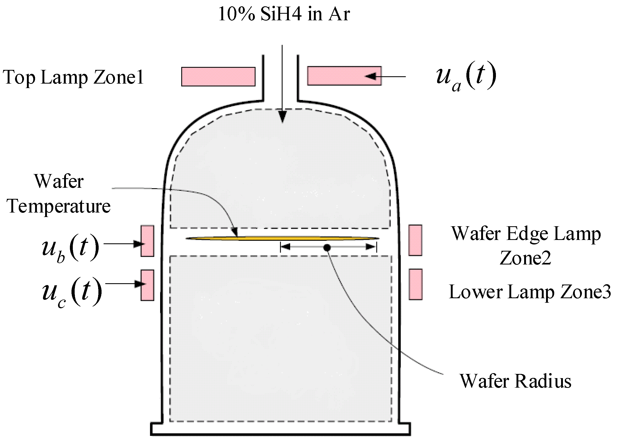
The Rapid Thermal Chemical Vapor Deposition (RTCVD) system is an advanced deposition technology commonly used in semiconductor and materials processing [
19]. This system combines the principles of chemical vapor deposition with rapid thermal processing (RTP) to achieve high-quality thin film deposition at significantly higher speeds than traditional methods. In a typical RTCVD system, a 6-inch silicon wafer is placed on a rotating stage within the reaction chamber. The wafer is heated by a set of three independent light sources, each with specific functions: Zone 1 uniformly heats the entire wafer surface, Zone 2 heats the wafer edges, and Zone 3 provides almost uniform heating across the wafer. The precise control of the heat flux from these light sources ensures the rapid, yet controlled, temperature rise required for effective deposition. The diagram of the RTCVD is shown in
Figure 1.
During the process, silane (SiH4) gas is introduced into the reactor, where it decomposes into silicon and hydrogen. At temperatures of approximately 800 K or higher, a 0.5 μm thick polysilicon layer is deposited on the wafer within a very short time, typically around 1 min. The rotating stage serves to maintain uniform temperature distribution across the wafer, with particular attention to the wafer radial temperature uniformity. Due to the thin nature of the silicon wafer, the temperature variation across the wafer’s azimuthal direction can be neglected. However, to achieve uniform polysilicon deposition, it is critical to maintain a consistent temperature across the wafer radius. This is achieved by adjusting the power levels of the three heating zones (light groups), which are carefully controlled during the deposition process.
The system is modeled using a one-dimensional PDE that describes the temperature and deposition dynamics, simplified from the underlying multidimensional thermodynamic processes. This model allows for accurate predictions of temperature and film thickness, crucial for optimizing process conditions and improving film uniformity. The real-time control of temperature, deposition rate, and material properties is challenging due to the system’s nonlinear spatiotemporal dynamics. The rapid changes in both spatial and temporal domains demand high-precision modeling to ensure uniform deposition and high-quality thin films. The dimensionless partial differential equation description of the RTCVD system is as follows:
Subject to the boundary conditions as follows:
where
denotes dimensionless wafer temperature.
dimensionless radial position, normalized by the wafer radius
,
is the thermal conductivity of the wafer.
is the radiation coefficient of the quartz chamber.
is the wafer density.
,
,
: thermal radiation flux distributions in the radial direction from the three heating zones.
,
,
: control inputs for the respective heating zones.
is the radiation coefficient of the wafer.
is the incident radiation flux at the wafer edge.
The RTCVD system is a complex spatiotemporal system with infinite dimensionality. For practical purposes, only a finite number of sensors are used to measure the system output. Assume that the sensors are located at positions [, …, ], which captures the system output. The spatial domain is represented by the vector . At each time step , the spatial output is given by the vector: . The temporal input is denoted by , where is the time variable. The objective of the modeling problem is to develop a spatiotemporal model based on the input data and the output data , where is the length of the time series. The model aims to capture the spatiotemporal dynamics of the system.
3. 3D Fuzzy Modeling Based on Automatic Clustering and HELM
The 3D fuzzy modeling method proposed in this section combines automatic clustering based on GA and HELM to effectively model complex systems with spatiotemporal dynamic characteristics. This method fully utilizes the advantages of each component to accurately capture the spatial and temporal relationships of the system while avoiding the limitation of dimensionality reduction.
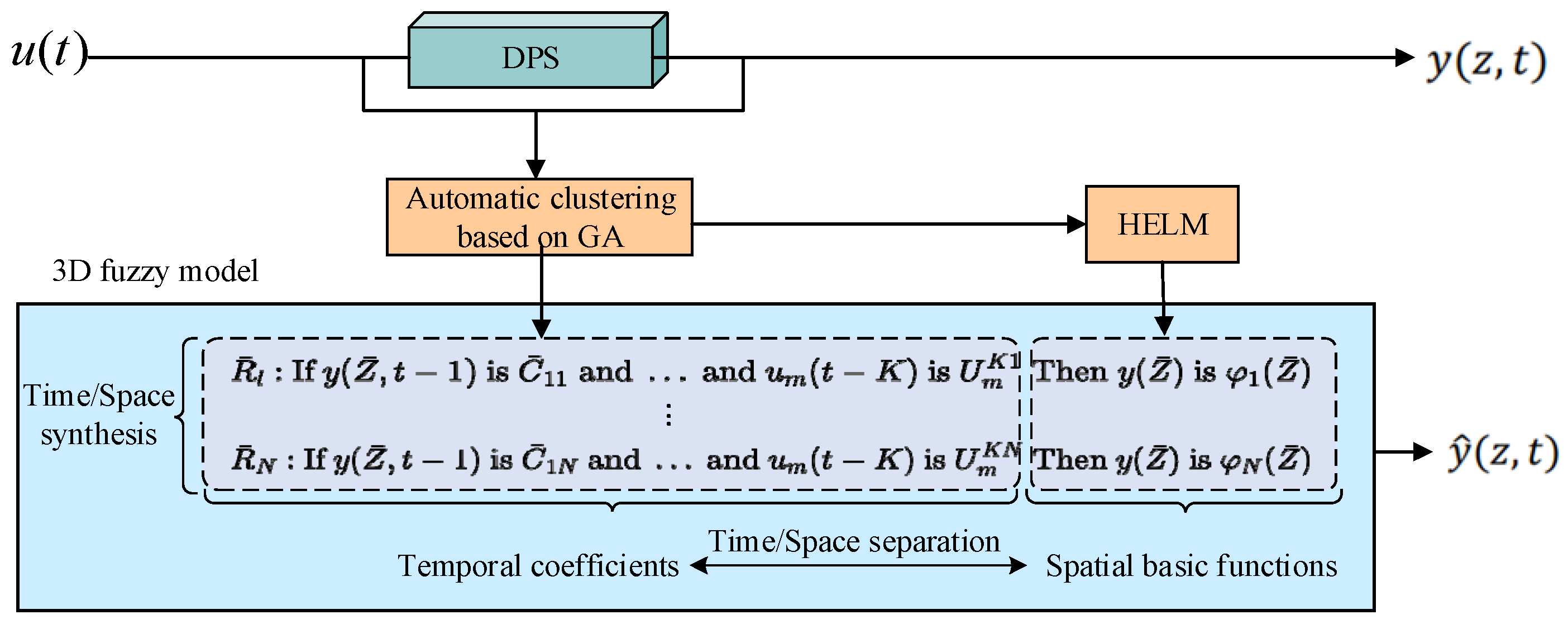
The proposed 3D fuzzy modeling method is shown in
Figure 2. First, the premise part of the fuzzy rule is learned by applying automatic clustering techniques, which are optimized using GA. Specifically, the GA is employed to guide the clustering process, ensuring that the fuzzy rules are constructed based on the optimal division of the input data. This process divides the input and output data into several clusters, each corresponding to a different mode of system behavior. Each cluster defines a fuzzy rule to describe the relationship between the input (spatial and temporal) and the output. The clustering process is optimized by GA, which not only reduces redundant rules but also improves the efficiency and adaptability of the model. Then, the spatial basis functions are learned using hierarchical ELM. The spatial basis functions learned by HELM can effectively represent the behavioral changes of the system at different spatial locations. After learning the premise part and spatial basis functions of the fuzzy rules, the final 3D fuzzy model combines the two to form a complete spatiotemporal modeling framework.
3.1. 3D Fuzzy Model
The 3D fuzzy model is an advanced modeling method for dealing with complex nonlinear DPS [
20]. Unlike traditional fuzzy models, the 3D fuzzy model does not rely on dimensionality reduction techniques and can directly model the dynamics of systems with spatiotemporal coupling, avoiding information loss [
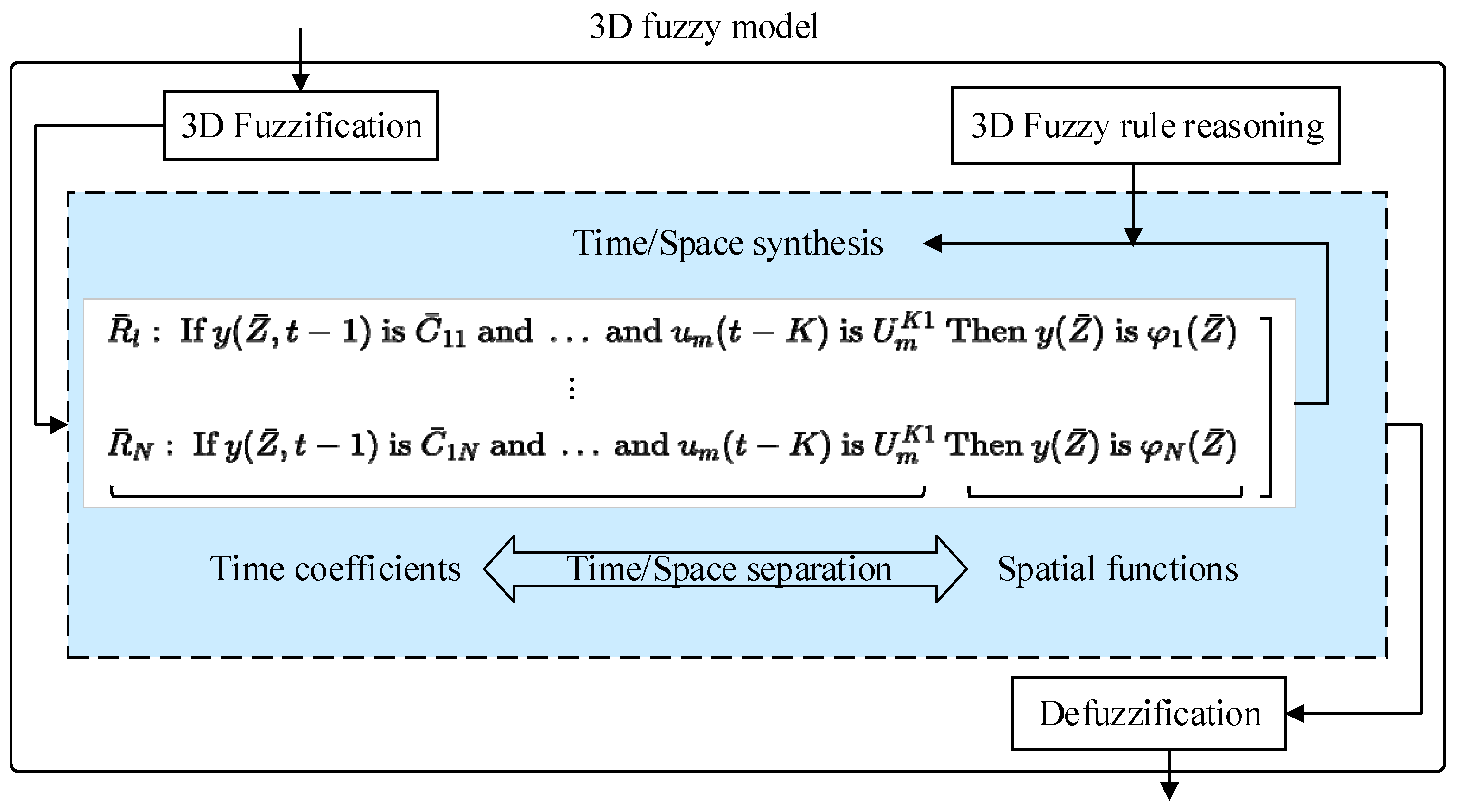
21]. The model is based on the concept of 3D fuzzy sets and can simultaneously represent changes in time and space dimensions. By treating time and space as closely related variables, the 3D fuzzy model can comprehensively capture the behavioral changes of the system at different time points and spatial locations. The 3D fuzzy modeling framework is shown in
Figure 3. A detailed description of the 3D fuzzy model is given in the
Appendix A.
The core advantage of the 3D fuzzy model is that it can preserve the complexity of the system without loss. It combines spatiotemporal separation with spatiotemporal reconstruction to achieve a coordinated modeling framework. The 3D fuzzy model can describe the DPS using the following 3D fuzzy language rules.
where
and
are taken as the input variables for a 3D fuzzy system.
and
are the 3D fuzzy set and the traditional fuzzy set, respectively.
is a spatial basis function, and
is the space domain.
is the order of the model.
is the number of fuzzy rules.
For each 3D fuzzy rule , the premise is used to compute the temporal coefficient, while the consequence represents the spatial basis functions. Thus, the fuzzy rule inherently realizes spatiotemporal separation. When multiple 3D fuzzy rules are activated simultaneously, their union generates the fuzzy output of the 3D fuzzy model, thereby naturally achieving spatiotemporal synthesis.
3.2. GA-Based Automatic Clustering Learning for the Premise Part
In 3D fuzzy systems, the premise part determines the input part of the fuzzy rules. Its main task is to automatically determine the best clustering center based on the characteristics of the input data. The main challenge is how to determine the optimal number of 3D fuzzy sets in the premise part and their corresponding membership functions. Traditional methods often rely on manual adjustment or prior knowledge, which may not be feasible in the case of complex systems and large-scale data sets. This paper uses the GA-based automatic clustering learning premise part to automatically optimize 3D fuzzy rules. The detailed process of automatic clustering based on GA is given below.
- (1)
Initializing the Population
The first step is to generate the initial population. Each individual represents a clustering structure, consisting of a set of clustering centers . The initial clustering centers are randomly selected from the data points.
- (2)
Fitness Evaluation
The fitness of each individual is evaluated using a clustering quality measure, such as the Davies–Bouldin (DB) index. This is performed by calculating the distance matrix
between the data sets
and the clustering centers
. Each data point
is assigned to the nearest clustering center
, and the minimum distance
is calculated. Based on this, the spread of each cluster
is computed, and then the relative spread
between clusters is calculated along with the DB index. The specific calculations are as follows.
where
is the number of data points assigned to cluster
, and
is the Minkowski distance parameter.
is the distance between clusters
and
, k is the number of clusters, and
is the relative spread between clusters
and
. The fitness of each individual is given by the DB index value. A higher fitness indicates a better clustering result, meaning that the clustering centers and their weights more effectively describe the structure of the data.
- (3)
Selection and Crossover
In the selection process, roulette wheel selection is used to select parent individuals. The higher the fitness (i.e., the lower the DB index), the greater the probability that the individual will be selected. The selection probability is calculated as follows.
where
is the fitness of the
-th individual.
is the largest fitness value in the current population.
is a parameter used to adjust the steepness of the selection.
is the total number of individuals in the population.
The purpose of the crossover operation is to generate new offspring individuals by combining the genes of two parent individuals, promoting extensive exploration of the knowledge space. The crossover operation retains the advantages of the parents while combining the genetic information of the two parents to provide more potential solutions. The crossover operation generates new offspring individuals by weighted average. First, a weight matrix
is randomly generated. The random number matrix
determines the weight of the combination of genes of two parent individuals. The introduction of the weight matrix
makes the crossover process more flexible and can generate different offspring according to different parent information. This operation can effectively avoid premature convergence of the algorithm. Then, gene recombination is performed. For the two parent individuals, the two offspring are calculated by weighted average. The specific calculation process is as follows.
where
is a random value drawn from a uniform distribution in the range [
] and
controls the randomness and diversity of the crossover process.
where
acts as a weight factor between the two parent individuals.
,
are two parent individuals,
,
are two offspring individuals.
- (4)
Mutation
The purpose of the mutation operation is to introduce random changes in the genes of individuals to prevent the algorithm from falling into a local optimal solution during the search process. Randomly select parent individuals for random perturbation to generate mutated individuals. For each gene position
, the mutated gene value
is calculated as follows.
where
is the number of genes that need to be mutated,
is the mutation rate.
is the disturbance amplitude, which determines the range of variation.
is the number of genes in an individual.
and
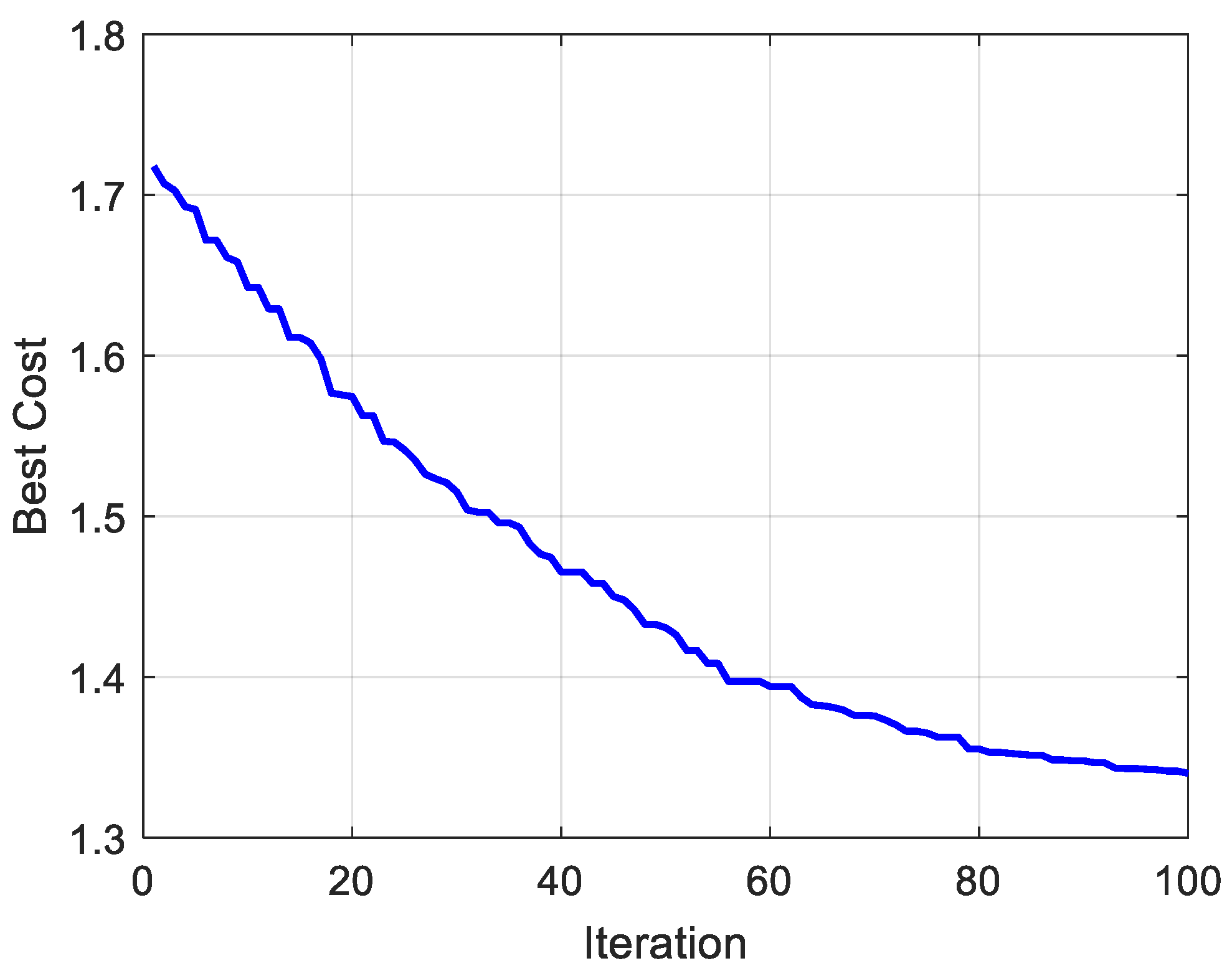
are the maximum and minimum values of the decision variables, respectively. The iterative change process of the fitness function is shown in
Figure 4. The specific parameter values are shown in
Table 1.
After automatic clustering,
is divided into
groups and
is the number of clusters. Each group is a cluster, each cluster corresponds to a 3D fuzzy rule, and
3D fuzzy rules are obtained. The cluster center constitutes the premise part of the 3D fuzzy rule. This paper adopts the Gaussian membership function, and the cluster center corresponds to the center of the Gaussian membership function in the premise part. The calculation method of the time coefficient (also called a fuzzy basis function in the context of the 3D fuzzy system) of the premise part is as follows.
where
and
represent the center and width of the Gaussian 3D fuzzy set
,
and
represent the center and width of the traditional Gaussian fuzzy set
3.3. Learning the Consequent Part Based on HELM
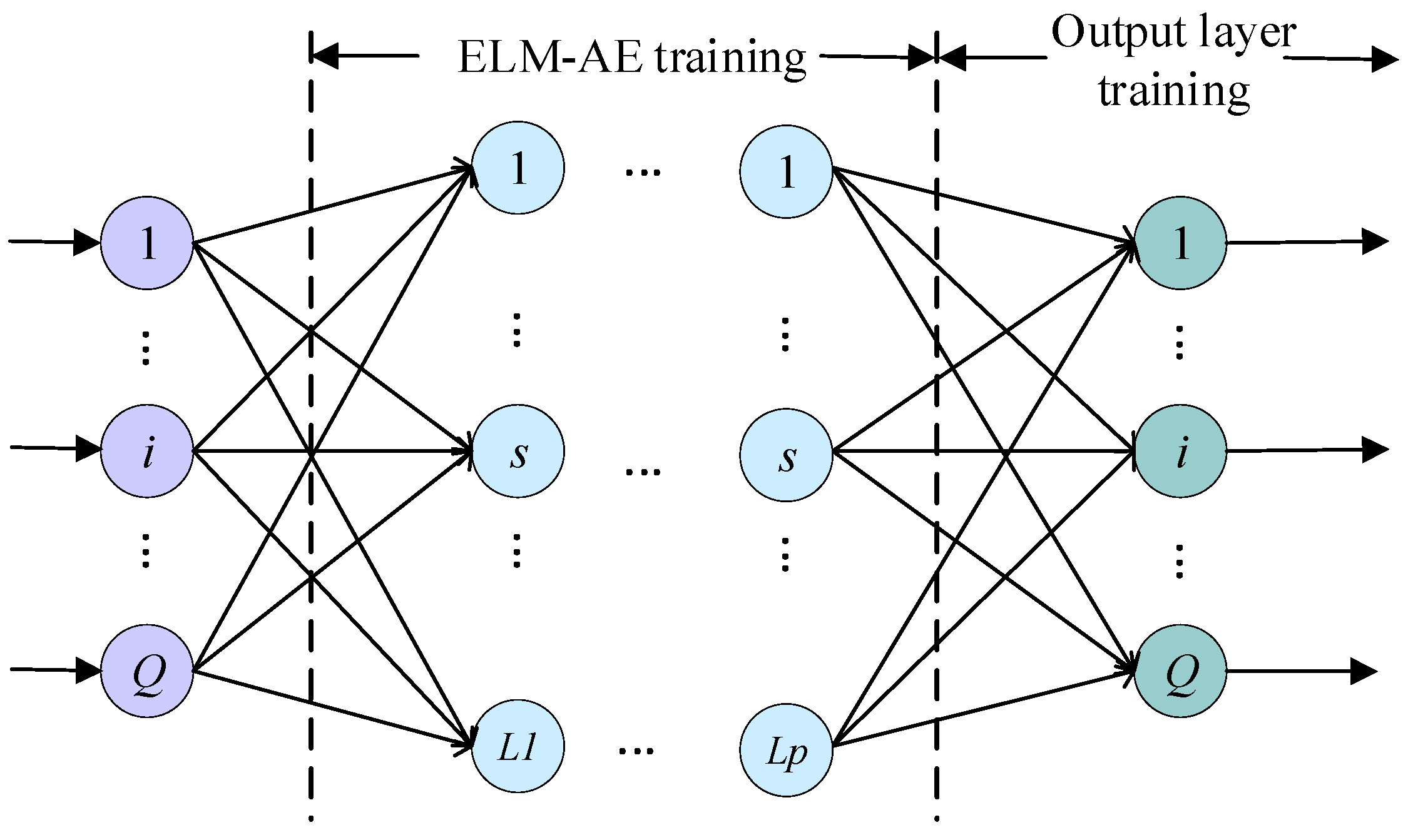
HELM is a neural network model based on a hierarchical structure, which combines the advantages of ELM and introduces the structure of the autoencoder (AE) hierarchy. The architecture consists of multiple autoencoder layers (ELM-AE layers) and an output layer [
22,
23]. HELM implements feature learning and mapping through multiple layers of ELM-AE layers, and can effectively handle complex nonlinear problems. The architecture includes an input layer, multiple hidden layers, and an output layer. The input layer receives the original data and performs linear transformation and nonlinear activation through each layer of the ELM-AE layer to gradually extract the high-level features of the data. Each ELM-AE layer contains input weights, biases, and output weights, and its parameters are trained through unsupervised learning to gradually capture richer feature representations in multiple levels. Finally, the output layer optimizes the output weights through supervised learning and combines the features of all hidden layers for final prediction. The HELM framework structure is shown in
Figure 5.
In the ELM-AE training phase, the autoencoder (ELM-AE) of each layer is trained. Each layer is linearly transformed by the input data and input weights, and a nonlinear activation function (ELU) is applied to generate the feature representation of the layer. In this way, the model gradually extracts high-level features of the data. During the training of each layer, the output weights are updated and the features of the layer are passed to the next layer. Then, the model enters the output layer training phase. At this time, the weights of the output layer are optimized by the least squares method.
The motivation for using HELM to learn spatial basis functions lies in its efficient training mechanism and powerful nonlinear mapping ability, which can capture complex input–output relationships [
24]. The hierarchical structure enhances the representation and generalization capabilities of the model and is particularly suitable for processing systems with spatiotemporal nonlinear characteristics. Through layer-by-layer feature learning, HELM not only reduces computational complexity but also improves the adaptability and interpretability of the system.
The training process of HELM maintains the high efficiency of ELM. The weights of the hidden layer are randomly selected, avoiding the computational complexity of backpropagation in traditional neural networks. Since the fuzzy rules directly correspond to the hidden layer nodes, the output of the system can be clearly linked to the consequent part of each fuzzy rule, which enhances the interpretability of the model.
In this study, HELM is used to learn the spatial basis functions of the consequent part. The size of the input layer is equal to the size of the input vector, and the number of nodes in the output layer and the hidden layer corresponds to the number of rules. The weight between the hidden layer and the output layer is called the -th spatial basis function. Each spatial basis function corresponds to the consequent part of a fuzzy rule. These weights learn the mapping between the input signal and the output signal in the rule. HELM can effectively represent spatial basis functions by learning weights.
The learning results of the premise part serve as the input of HELM. Specifically, given an input sample
, where each sample
is an input vector and
is the corresponding target output. For each hidden layer
(from the input layer to the penultimate layer), the input is the output from the previous layer. The hidden layer output matrix
is computed, where the elements are the activation values of the hidden nodes. The computation formula is as follows.
where
is the output of the previous layer,
is the input weight of the current layer,
is the bias, and
is the activation function.
For each layer
, the output weights
are computed using the least squares method, as follows.
where
is the regularization coefficient, and
is the identity matrix.
For each layer
, the output from the previous layer is used as the input for the current layer. The hidden layer output matrix
and output weights
are computed sequentially. For the final layer
, the output weights
for the last layer are computed directly using the least squares method:
where
is the hidden layer output matrix for the final layer, and
is the final target output.
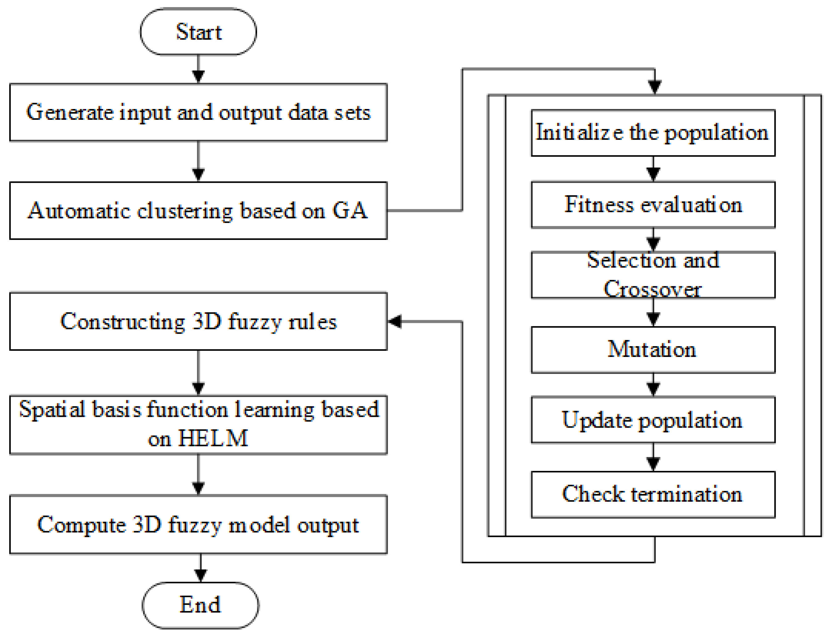
The proposed 3D fuzzy modeling flowchart is shown in
Figure 6. The output model of the online 3D fuzzy system is as follows.
where
is the temporal coefficient,
is the spatial basis function.
4. Experimental Validation
The RTCVD described in
Section 2 is used to evaluate the effectiveness of the proposed modeling approach. In this experiment, random disturbances with amplitudes no greater than 10% were applied to the system input variables
to capture sufficient dynamic information. Specifically, the disturbed inputs can be expressed as follows:
where
simulates the random direction of the disturbance signal. This approach effectively simulates the fluctuations of input variables and enhances the dynamic response of the system.
Additionally, 11 sensors were uniformly distributed along the radial direction for data acquisition. To simulate noise effects in real-world operation, independent Gaussian white noise with zero mean and a standard deviation of was added to the sensor data. The inclusion of noise introduces uncertainty into the experimental data, enhancing the model’s robustness to disturbances and errors, and thereby improving the practical representativeness of the experimental results. Under steady-state conditions, the values of , , and are 0.2028, 0.1008, and 0.2245, respectively, corresponding to the stable input values at a furnace temperature of 1000 K. These steady-state values serve as the baseline inputs, with disturbances applied on top of them.
In this study, the sampling interval was set to 0.5 s, with a total simulation period of 2500 s. Consequently, 5000 samples were generated. Among these, 2000 samples were randomly selected for training experiments, and another 500 samples were randomly chosen for testing experiments.
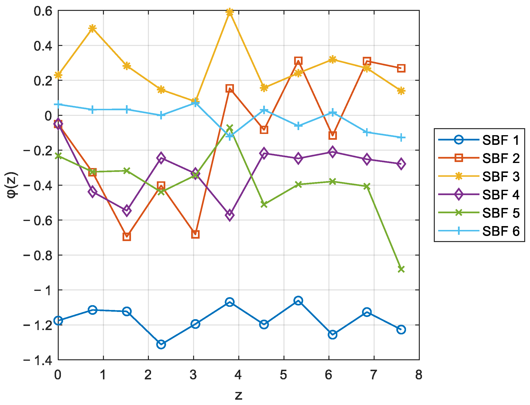
The premise part of the 3D fuzzy rules is learned through the GA-based automatic clustering method. The data set is divided into 13 groups to determine the input space of the premise part of the rule base. Specifically, the GA-based automatic clustering method automatically divides the input data into 13 different categories, each of which corresponds to a fuzzy rule. These 13 fuzzy rules are generated through automatic clustering to ensure that each rule can effectively reflect the different characteristics of the input data. Subsequently, the weights of the output layer are learned through HELM to obtain 13 spatial basis functions. By combining the premise part with the consequent part, a complete three-dimensional fuzzy rule base is constructed, which contains 13 fuzzy rules. The first six three-dimensional fuzzy rules are listed below.
| is [−1.1756 −1.1146 −1.1229 −1.3121 −1.1951 −1.0693 −1.1978 −1.0612 −1.2563 −1.1267 −1.2271]; |
| is [−0.0504 −0.3260 −0.6957 −0.4022 −0.6820 0.1543 −0.0835 0.3123 −0.1161 0.3101 0.2692]; |
| is [0.2303 0.4975 0.2830 0.1465 0.0785 0.5908 0.1568 0.2411 0.3195 0.2691 0.1395]; |
| is [−0.0494 −0.4380 −0.5462 −0.2444 −0.3338 −0.5723 −0.2176 −0.2473 −0.2097 −0.2519 −0.2786]; |
| is [−0.2324 −0.3239 −0.3178 −0.4397 −0.3438 −0.0708 −0.5105 −0.3961 −0.3791 −0.4069 −0.8812]; |
| is [0.0625 0.0325 0.0335 −1.8757 0.0708 −0.1220 0.0312 −0.0611 0.0167 −0.0973 −0.1266]. |
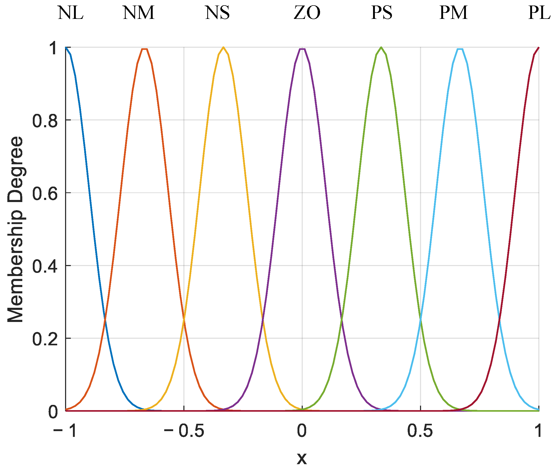
The fuzzy set of each input variable is represented by a Gaussian membership function, where NB represents negative big, NM represents negative middle, NS represents negative small, ZO represents zero fuzzy set, PS represents positive small, PM represents positive middle, and PB represents positive big. The membership function of the premise part of the 3D fuzzy rule is shown in
Figure 7.
The first six spatial basis functions are shown in
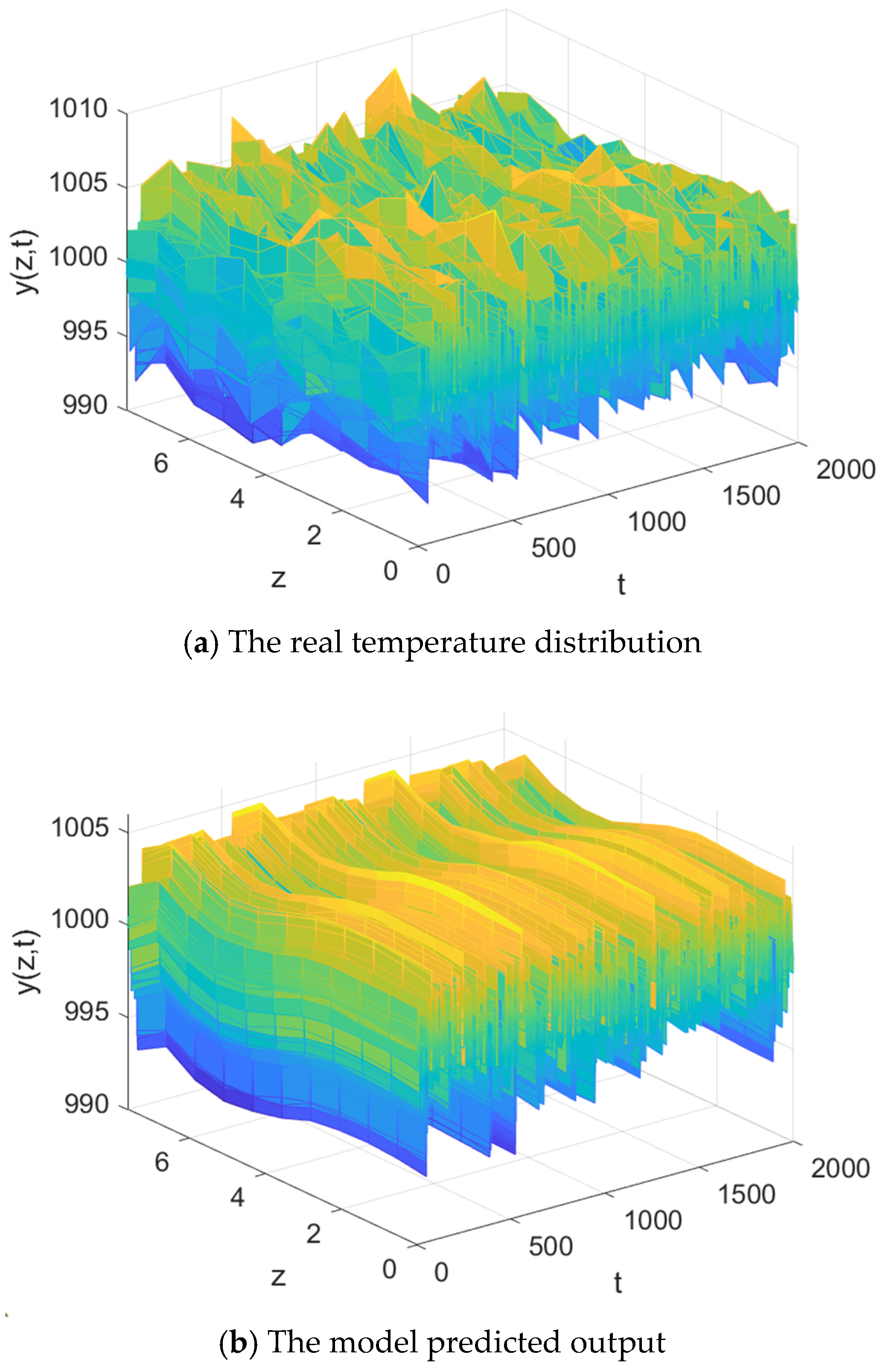
Figure 8. The true output and prediction results of the proposed model method in 2000 training samples are shown in
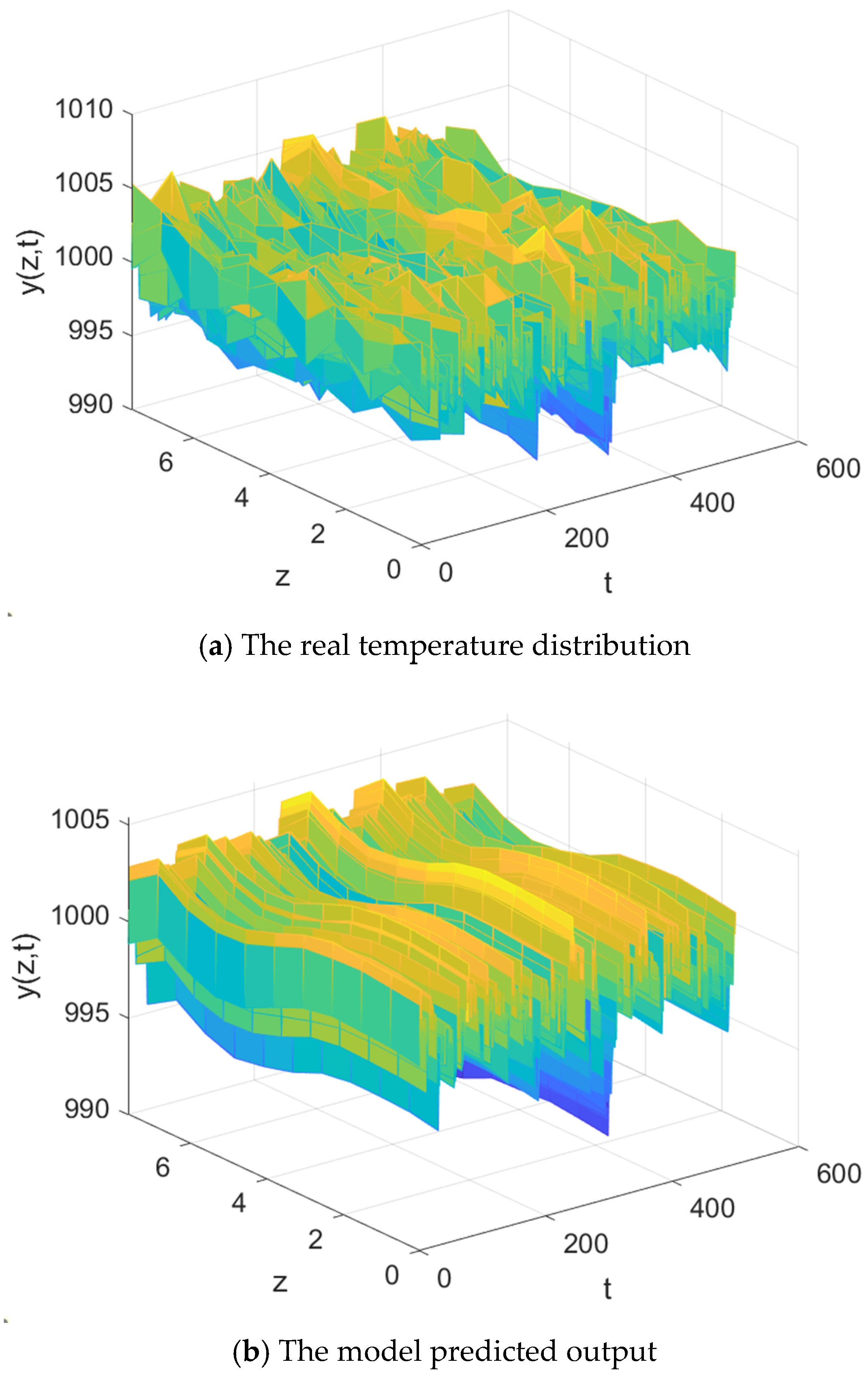
Figure 9, and the true output and prediction results of the model in 500 test samples are shown in
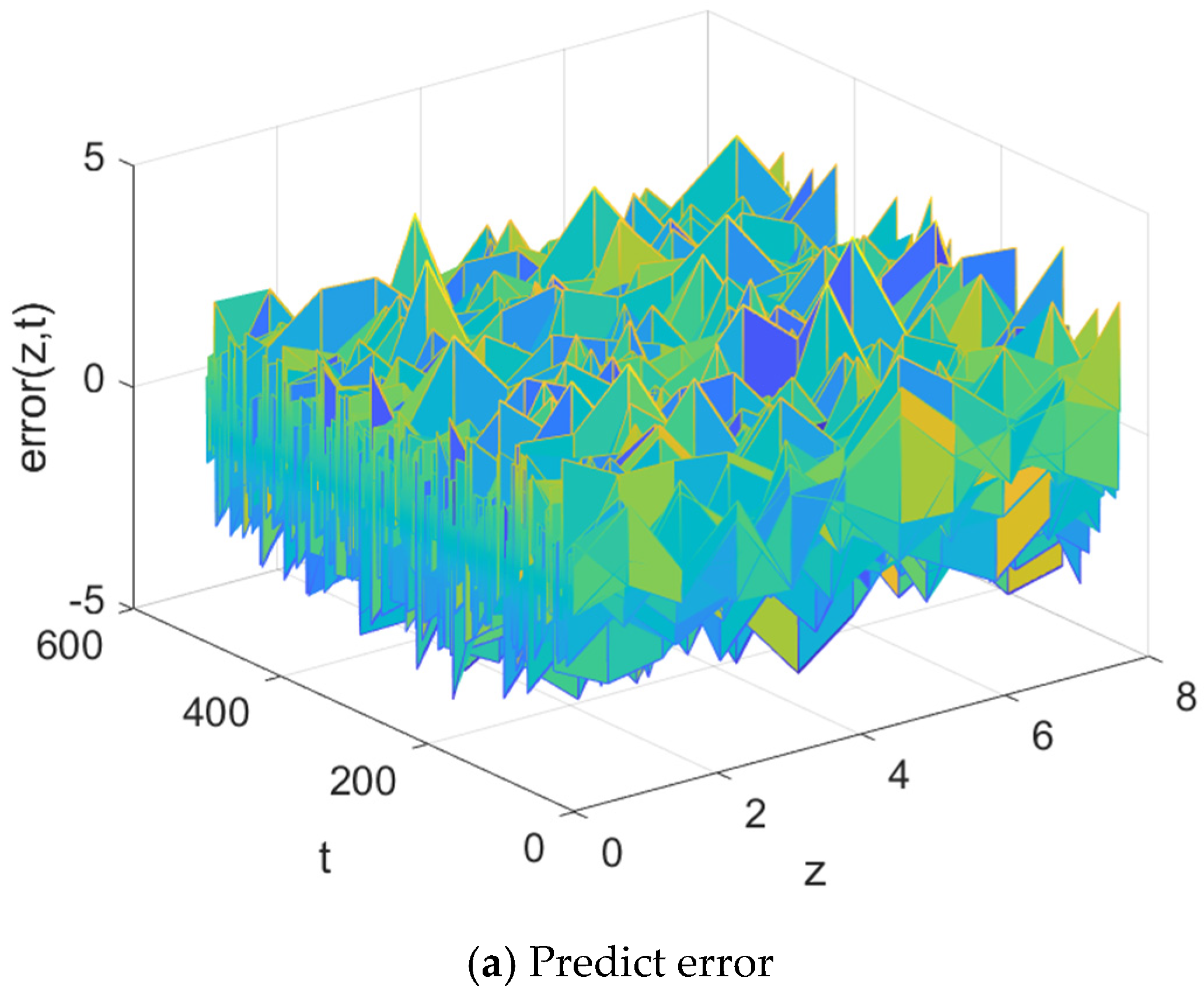
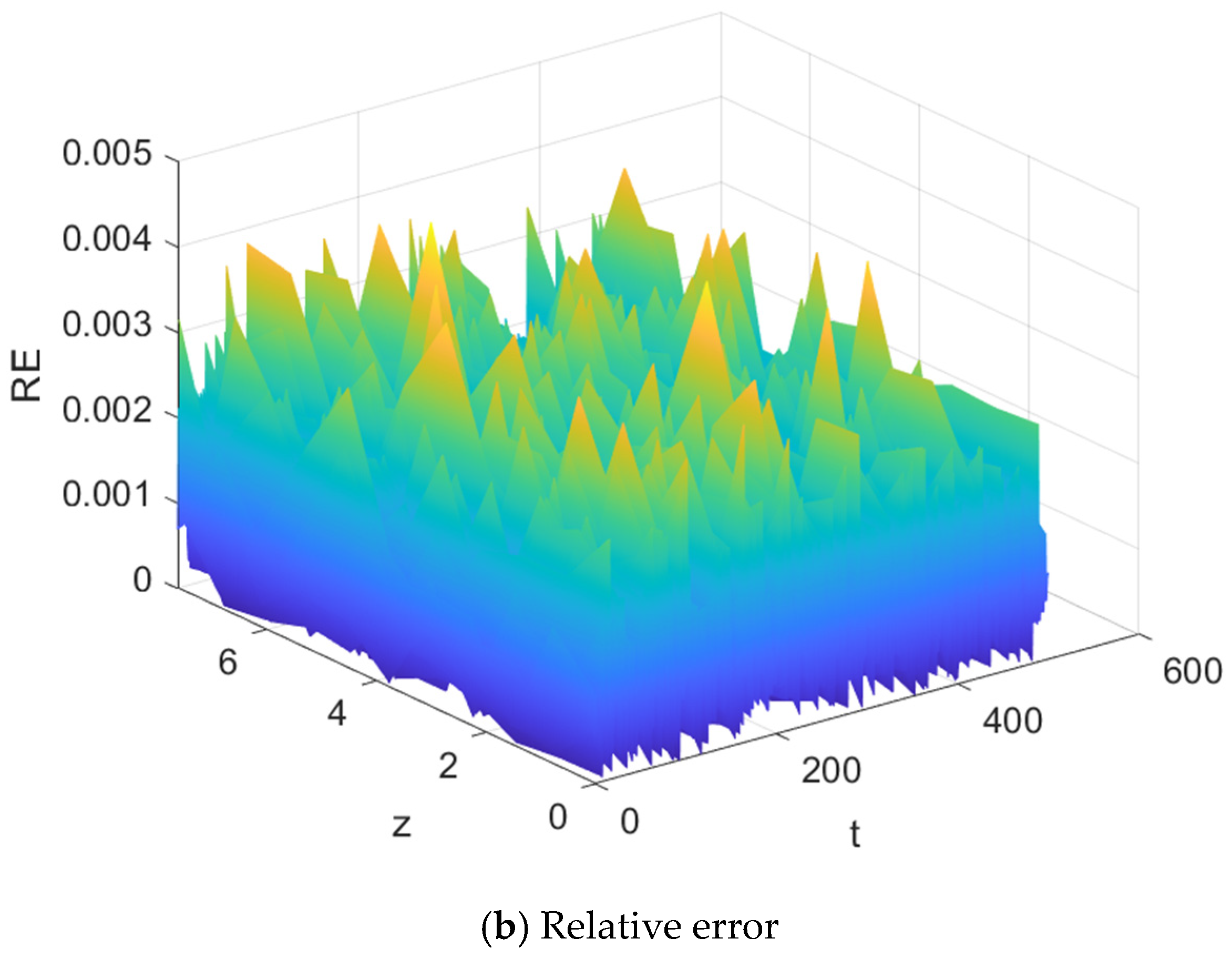
Figure 10. The prediction error and relative error of the proposed modeling method are shown in
Figure 11. The results show that the spatial distribution of the predicted output can well match the true temperature distribution. The matrix representations of the first six spatial basis functions are shown below.
The proposed modeling method was compared with two existing methods, including KL-LS [
25] and KL-LS-SVM [
26], to verify the performance of the proposed modeling method. The KL-LS modeling approach effectively models the dynamics of DPS by combining the Karhunen–Loeve (KL) decomposition and least squares estimation (LS). It first uses KL decomposition to transform the infinite-dimensional output of the system into a finite-dimensional approximation, capturing the spatial correlation of the system through spatial basis functions. This reduction allows the extraction of time-varying coefficients, which are then identified through least squares estimation and instrumental variables to establish the dynamic relationship between the system input and output. This method can accurately model spatial and temporal behavior even under nonlinear conditions. The effectiveness of the method has been demonstrated through simulations of parabolic and hyperbolic systems, highlighting its ability to simulate complex spatiotemporal dynamics in various distributed processes with improved computational efficiency and accuracy.
The KL-LS-SVM is a time/space separation based SVM model identification method for unknown nonlinear DPS. The method first uses KL decomposition to separate the time and space domains and reduce the dimensionality of the system. Then, the spatiotemporal outputs are projected onto the low-dimensional KL space, and the time coefficients capture the dynamics of the system. A least squares support vector machine is used to model the system in this simplified time domain. After integrating the time and space components, the nonlinear spatiotemporal dynamics of the system can be reconstructed. The parameters of all comparison methods are set according to the original text.
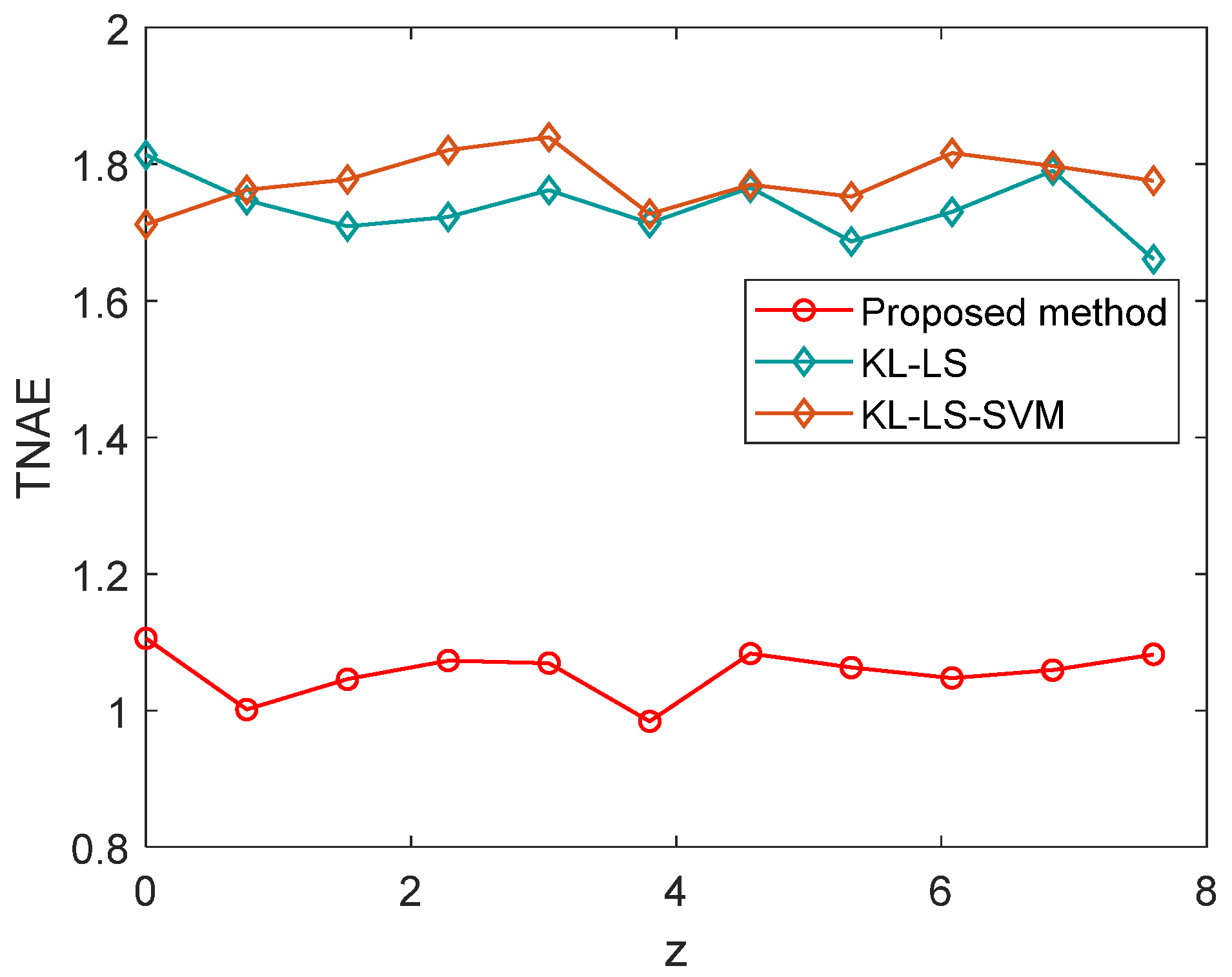
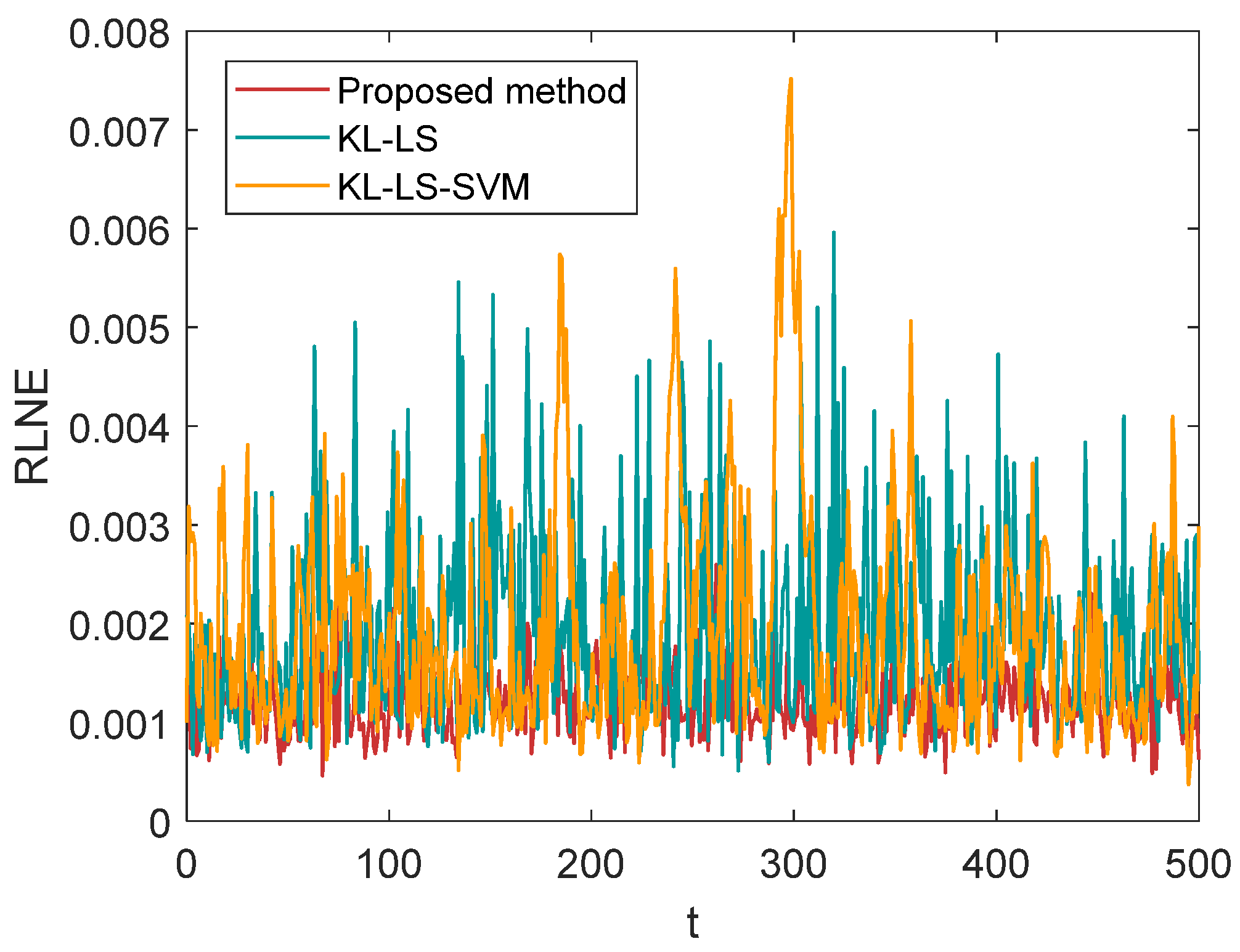
Figure 12 and
Figure 13 compare their performance in time normalized absolute error (TNAE) and relative
norm error (RLNE), respectively. The experimental results in
Figure 12 show that the proposed method has lower error than the other methods at all sensor locations. The RLNE results in
Figure 13 show that the proposed method performs better than other methods with good stability.
Table 2 shows the root mean square error (RMSE) of the compared methods in the training and testing stages. For a reliable performance evaluation, we performed the experiments 10 times with different random data splits. The RMSE values were then averaged across all 10 repetitions to ensure that the results are not biased by the random variation in the data selection.
In summary, the proposed 3D fuzzy modeling approach successfully captures the spatiotemporal coupled dynamics of DPS by effectively combining the advantages of GA automatic clustering and HELM. GA-based automatic clustering can accurately divide input and output data and generate high-quality fuzzy rules, avoiding information loss and dimensionality reduction errors in traditional methods; HELM builds a complete three-dimensional fuzzy rule library by learning spatial basis functions, improving the accuracy and expression ability of the model. Experimental verification results show that this method can accurately predict the temperature distribution of RTCVD and shows good robustness under the influence of noise.


