Abstract
Spherical tanks are widely utilized in process industries due to their substantial storage capacity. These industries’ inherent challenges necessitate using highly efficient controllers to manage various process parameters, especially given their nonlinear behavior. This paper proposes the Approximate Generalized Time Moments (AGTM) optimization technique for designing the parameters of multi-model fractional-order controllers for regulating the output (liquid level) of a real-time nonlinear spherical tank. System identification for different regions of the nonlinear process is here innovatively conducted using a black-box model, which is determined to be nonlinear and approximated as a First Order Plus Dead Time (FOPDT) system over each region. Both model identification and controller design are performed in simulation and real-time using a National Instruments NI DAQmx 6211 Data Acquisition (DAQ) card (NI SYSTEMS INDIA PVT. LTD., Bangalore Karnataka, India) and MATLAB/SIMULINK software (MATLAB R2021a). The performance of the overall algorithm is evaluated through simulation and experimental testing, with several setpoints and load changes, and is compared to the performance of other algorithms tuned within the same framework. While traditional approaches, such as integer-order controllers or linear approximations, often struggle to provide consistent performance across the operating range of spherical tanks, it is originally shown how the combination of multi-model fractional-order controller design—AGTM optimization method—GA for expansion point selection and index minimization has benefits in specifically controlling a (difficult to be controlled) nonlinear process.
Keywords:
AGTM optimization; multi-model fractional-order controllers; nonlinear system; spherical tank MSC:
93B52
1. Introduction
Many process industries face significant control challenges due to the nonlinear dynamics of their operations. This inherent nonlinearity often necessitates traditional control methods, especially in petrochemicals, food processing, pharmaceuticals, papermaking, and water treatment. Spherical tanks, commonly used in these industries, present challenges for level control due to their varying cross-sectional area and nonlinear behavior. Liquid level control systems are crucial across various fields, but accurately modeling them is often difficult. Neglecting model accuracy can lead to failures, particularly in highly nonlinear regions [1]. The increasing interest in nonlinear models highlights their advantages in representing process dynamics over broader ranges [2]. These models, typically derived from first principles and refined with process data, are still being improved. Once the model is established, designing a controller becomes essential to maintain process stability. The Proportional Integral Derivative (PID) controller is a widely recognized component in process control and remains extensively used despite advancements in control theory. Its simplicity, cost-effectiveness, ease of design, and robustness, especially in linear systems, make it popular in the industry [3]. As control engineering evolves, the pursuit of better and simpler control algorithms continues. In the past decade, research into fractional calculus [4,5,6] and its applications in control theory has significantly increased [7,8,9,10]. In practical control scenarios, fractional-order controllers are increasingly favored, particularly when the plant model has already been established in the classical sense as an integer-order model. From an engineering standpoint, the primary objective revolves around enhancing or optimizing performance. Therefore, we aim to employ Fractional-Order Control (FOC) to enhance the control performance of integer-order dynamic systems. Groundbreaking research on the application of fractional calculus in dynamic systems and controls, as well as recent developments, are detailed in [7,11,12,13,14,15,16].
The following literature presents a range of control strategies designed for various spherical tank configurations. Ashwini et al. [17] developed the Fuzzy Deep Neural Sliding Mode Fractional-Order Proportional Integral Derivative (FDN-SM-FOPID) controller to regulate liquid levels in nonlinear quadruple spherical tank systems in real-time, utilizing the backpropagation algorithm. Building on this, Jegatheesha and Kumar [18] developed an innovative Fuzzy FOPID (FFOPID) controller for a nonlinear interacting coupled spherical tank system to effectively manage the level process. Arivalahan et al. [19] then advanced the field further by developing a FOPID controller for regulating liquid levels in a spherical two-tank system, using a hybrid approach that integrated Chaotic Henry Gas Solubility Optimization (CHGSO) with Feedback Artificial Tree (FAT). In the context of multi-tank systems, Debnath and Mija [20] employed Particle Swarm Optimization (PSO) to develop a Brain Emotional Learning-Based Intelligent Controller (BELBIC) for a Quadruple Tank System (QTS). Similarly, Jáuregui et al. [21] applied PSO to implement a FOPID controller for level control in a conical tank. Extending the focus to different methodologies, Meng et al. [22] proposed an input/output feedback linearization control with a Nonlinear Disturbance Observer (NDOB) to regulate the Quadruple-Tank Liquid Level (QTLL) process, while Huo et al. [23] applied the Plug-and-Play (PnP) process monitoring and control method to a real-time three-tank system. Das et al. [24] contributed by designing a fractional dual-tilt derivative controller for a two-tank system, with parameters computed using gain and phase-margin specifications. Tao Xu et al. [25] further explored control strategies by proposing an adaptive L2 control method using the Port Controlled Hamiltonian (PCH) model to manage a Two-Tank Liquid Level System (TTLLS) under parameter uncertainties and disturbances. Fu et al. [26] also focused on adaptive strategies, developing a dual-rate adaptive decoupling controller for a dual-tank water system using polynomial transformation and a recursive least squares algorithm. Transitioning to IoT applications, Bhookya et al. [27] developed a real-time system for controlling liquid levels in a cylindrical tank using a PID controller optimized with a modified Grey Wolf Optimization (mGWO) algorithm. In a similar vein, Sreekanth and Nageswara [28] proposed an adaptive fractional-order controller for liquid level regulation in a Liquid Level Plant (LLP) using a frequency domain approach. Wang et al. [29] made significant strides in deep learning applications, developing a Deep Learning-based Model Predictive Control (DeepMPC) for level control in Continuous Stirred-Tank Reactor (CSTR) systems, utilizing a Growing Deep Belief Network (GDBN). Following this, Matušů et al. [30] proposed a robust PI control strategy for the CSTR, employing the stability boundary locus method and the sixteen-plant theorem. Building on these advancements, Alshammari et al. [31] introduced an Adaptive Fuzzy Gain Scheduling PID (AFGS-PID) controller for temperature tracking in a CSTR. Finally, Chakravarthi and Venkatesan [32] developed an Adaptive Model-Based Gain Scheduled (AMBGS) Controller for a Single Spherical Nonlinear Tank System (SSTLLS) using LabVIEW, incorporating methodologies from Skogestad and Ziegler-Nichols (ZN).
Progress in control design for nonlinear systems has been significantly influenced by model-matching techniques [33,34]. The reference model selection process described in [35] includes specific time-domain criteria. Controller design for single-input single-output (SISO) systems was outlined in [36]. For multiple-input multiple-output (MIMO) systems, model-matching techniques have addressed various control challenges, including the design of controllers for both stable [37] and unstable [38] plants, the creation of robust decentralized controllers for stable and non-minimum phase plants [39], disturbance rejection [40], and the establishment of a damping-based controller design framework [41]. The importance of Time Moments (TM) and Markov Parameters (MP) in controller design is highlighted in [42], emphasizing their role in aligning the transient and steady-state responses of the reference system with the closed-loop configuration. The optimal combination of TM and MP for critically damped and underdamped systems is explored in [43,44]. Despite the simplicity of this approach, automating the process, however, remains challenging due to the complexities of expansion and inversion. Jayanta Pal [45] proposed an innovative method for model order reduction in the frequency domain. This approach introduces two new variables, AGTM and Approximate Generalized Markov Parameters (AGMP), to establish a stable lower-order structure for higher-order systems by achieving frequency integration between them. This technique offers a range of reduced-order models from various expansion points, providing users with multiple options for selecting a stable reduced-order model. Beevi et al. [46] developed a general Two Degree of Freedom (2-DOF) controller for time-delay systems utilizing the AGTM/AGMP optimization method.
This paper moves within the AGTM optimization method, explaining its principles and showcasing its application in improving both fractional-order when compared to standard controllers for the multi-model spherical tank. In particular, the original contribution of the paper lies in showing how the combination of multi-model fractional-order controller design—AGTM optimization method—GA for expansion point selection and index minimization has benefits in controlling a (difficult to be controlled) nonlinear process like the spherical tank (such an approach might be applied to other frameworks as well). Indeed, it provides a clear algorithmic flow to be generally followed in order to get rather satisfactory results in a rather complex control framework. It is worth remarking on how control failures in spherical tanks can have severe real-world consequences, highlighting the urgent need for advanced research. These tanks are crucial in industries such as petrochemicals, water treatment, and pharmaceuticals, where poor control can lead to process disruptions, inconsistent product quality, and costly downtime. Failures can also result in serious safety hazards, such as overfilling or leaks, potentially causing toxic spills, fires, or explosions. Additionally, environmental damage from chemical leaks and regulatory penalties can have long-term financial and reputational impacts. Frequent control issues also increase maintenance costs and energy consumption, while cascading failures in integrated systems can amplify operational risks.
The present work, which aims at definitely complementing [47] by resorting to a multi-model strategy, is organized into the following sections: The experimental model is presented in Section 2. Section 3 provides details on the control design. Section 4 discusses the Approximate Generalized Time Moments (AGTM) optimization technique. Section 5 elaborates on the outcomes obtained from implementing the AGTM optimization method for controller design in the spherical tank, analyzing the results of both simulations and experiments. Section 6 summarizes the key findings and contributions of the research presented in the paper. This study highlights the importance of the AGTM optimization method in resolving controller design challenges for spherical tanks and offers perspectives on potential future research avenues in this domain.
2. Experimental Modelization
As in [47] (the reader is referred to there for a more detailed characterization of the experimental framework), two spherical tanks are interconnected through a manually operated valve. Water is supplied to and drained from both tanks via a reservoir, with the flow regulated by pneumatic valves that are adjusted using air pressure from a compressor. The flow rate is manually controlled using a rotameter, and the liquid levels in the tanks are measured by a differential pressure transmitter providing a 4–20 mA signal output. In particular, the Rosemount 2051CD Differential Pressure Transmitter (DPT) (Emerson Process Management (India) Pvt. Ltd., Chennai, Tamil Nadu, India) is used, which offers several advantages in spherical tank liquid level control compared to other sensors such as Ultrasonic, Radar, Capacitance, Float Switches, Magnetostrictive, and Optical Level Sensors. It provides high accuracy (±0.05%) and reliability, even in pressurized or high-temperature environments, with built-in temperature compensation ensuring consistent performance. Unlike Ultrasonic and Radar sensors, which can be affected by foam, turbulence, or vapors, the DPT sensor calculates level accurately based on differential pressure, making it ideal for irregular shapes like spherical tanks. It also handles a wide range of fluids, including corrosive, viscous, and slurry-type liquids, outperforming Capacitance and Optical sensors that are sensitive to changes in fluid properties. The 2051CD’s rugged design ensures durability in harsh environments with vibration or corrosion, and its advanced diagnostics and digital integration capabilities surpass those of simpler sensors like Float Switches and Magnetostrictive sensors. While it requires knowledge of fluid density, its low maintenance and long-term stability make it a cost-effective and versatile solution for complex liquid level control. The NI-DAQmx 6211 data acquisition card, featuring a 10-volt range, 16 analog input channels, and 2 analog output channels, serves as the interface between the transmitter and the computer. This card offers a sampling rate of 250 kS/s and a resolution of 16 bits.
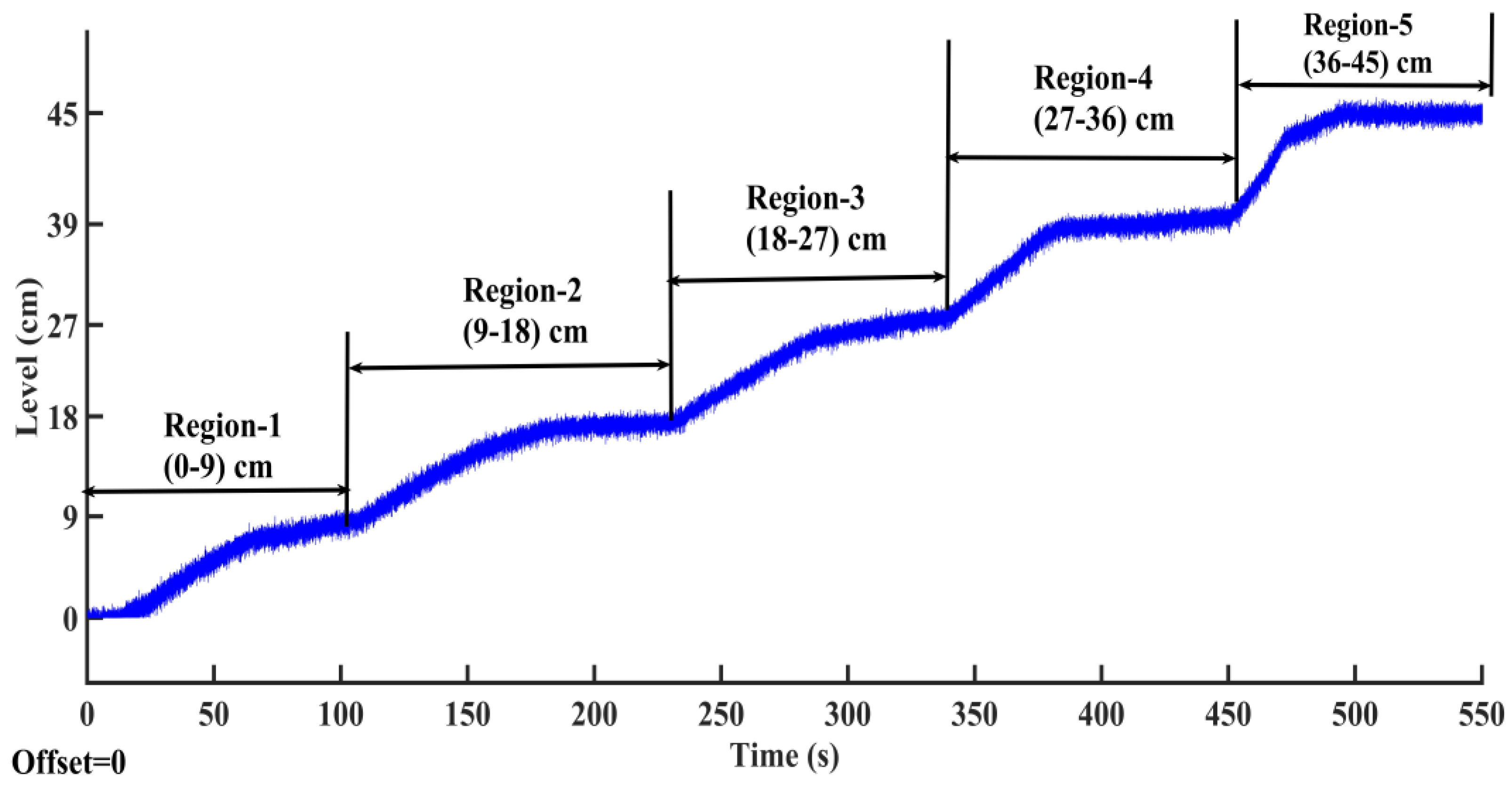
The process begins when the pneumatic control valve closes, adjusting the water flow into the tank using air. Data from the differential pressure transmitter, which measures water volume through a 4–20 mA current range, is collected by the NI-DAQmx 6211 data acquisition card. The computer calculates the control strategy and sends a signal to the I/P converter, which adjusts the pneumatic valve to control the water flow into the tank. This paper derives the plant model experimentally using a step input. By analyzing the step response data, we developed a precise model of the system dynamics. The step response curve in Figure 1 may exhibit an S-shape if the system lacks integrators or complex conjugate poles. The time constant and delay time are key parameters to describe this curve. After deriving the model, we designed and implemented both integer-order and fractional-order controllers using the AGTM optimization method to regulate the spherical tank parameters in real-time via the data acquisition device.

Figure 1.
Open-loop input–output response curve with an S-shaped characteristic.
The spherical tank process exhibits significant nonlinearity, primarily due to variations in the tank’s diameter. Experimental results indicate that changes in diameter contribute to the system’s nonlinearity, which can be described by a first-order differential equation. In accordance with the mass balance principle
the spherical tank model can be expressed as follows:
From now on, the time dependence is omitted for the sake of simplicity. Here is the cross-sectional area of the tank and the height of the tank in cm, is the inlet flow rate and is the outlet flow rate. The outlet flow rate is proportional to the square root of the liquid level due to gravitational effects on flow through an orifice,
where is the valve coefficient so that the resulting total mass balance yields a nonlinear dynamic model:
Now, let us develop the linearized approximation for this nonlinear model. The only nonlinear term in Equation (4) is . Take the Taylor series expansion of this term around a point h0
and, by neglecting terms of order two and higher, we get
which, if introduced in the nonlinear dynamic system (4), yields the following linearized approximate model:
when , namely the steady-state value of the liquid level for a given value of the inlet flow rate, is specifically considered, the linearized model around reads
at steady state from Equation (9) we also have ()
so that, by subtracting Equation (10) from (9), we obtain
by further defining the deviation variables
we take the following linearized form:
where .
Finally, by considering Laplace transforms, we write
so that the system transfer function reads
in terms of the time constant and the steady-state gain . Real-time identification of the spherical tank structure is performed using a black-box modeling approach, as in [47]. The tank is filled from 0 to 45 cm with steady water inflow and outflow rates. The NI-DAQmx 6211 collects individual samples via the USB port from the differential pressure transmitter, which operates within the 4 to 20 mA range. These data are then sent to the personal computer. Using the open-loop method, the system’s response to input variations is recorded. Sundaresan and Krishnaswamy [48] determined and by matching the process’s open-loop response to the model at two specific time instances. By analyzing the step response, the times and , which correspond to 35.3% and 85.3% of the response durations, were used to determine the time constant and delay,
at steady state, with consistent inlet and outlet flow rates, the process stabilizes. Subsequently, a step increment is introduced by adjusting the flow rate as shown in Table 1, and multiple measurements are taken until the system stabilizes, as depicted in Figure 1. The experimental data are approximated to the First Order Plus Dead Time (FOPDT) model, with parameters tailored for five operational regions within the spherical tank, balancing precision and complexity. The standard FOPDT model is as follows:
using the FOPDT model, transfer functions are derived for different regions. The total tank height is divided into five regions, each associated with a specific model detailed in Table 1, which provides transfer functions tailored to various sections within the spherical tank. Importantly, the delay increases exponentially with increasing nonlinearity. These transfer function models are formulated to address five distinct regions covering the varying diameters of the spherical tank. Spherical tanks have a curved design, which causes the cross-sectional area to change as the liquid level rises. The volume does not increase uniformly with height because the cross-sectional area is smaller at the top and bottom, leading to minimal volume changes for a given height variation. Conversely, the area is largest in the middle, resulting in more significant volume changes for the same height increase. Dividing the height of a spherical tank into five regions is essential to address the nonlinear relationship between height and volume, enhance control accuracy, and ensure safe and efficient operations. This segmentation is particularly important in applications requiring precise level control, as it enables the Differential Pressure Transmitter (DPT) to accurately interpret liquid levels despite the tank’s geometry.

Table 1.
Transfer function representations for various spherical tank regions.
3. Multi-Model Control Design
Integer-order controllers have been a fundamental element in control systems for decades, commonly applied in industrial processes due to their robustness and simplicity. The three adjustable control parameters here are proportional control , integral control , and derivative control gains. The mathematical expression defining the PID controller is presented as follows:
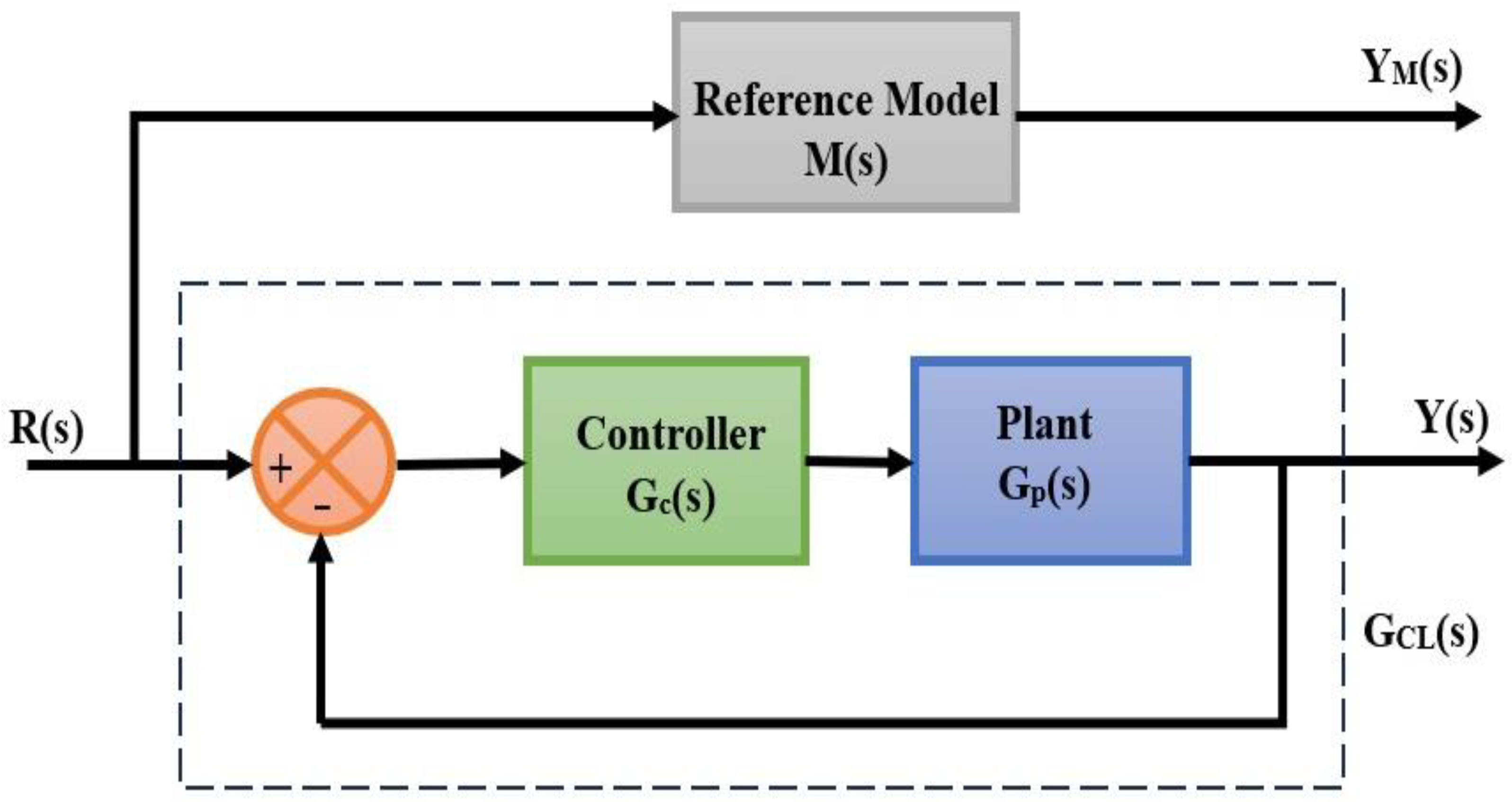
Extending the derivative and integrator orders from integers to fractional values offers a more flexible tuning mechanism for the fractional-order controller, making them a straightforward option for achieving control objectives compared to their integer-order counterparts [49,50,51]. The fractional-order controller outperforms the integer-order controller by tuning five parameters, offering enhanced robustness and control. These extra parameters enable more precise control and improved adaptability to system dynamics, leading to superior robustness and performance [52]. Such enhanced flexibility provides better disturbance rejection and adaptability to dynamic complexities compared to traditional PID controllers. These features make the FOPID controller highly suitable for addressing the nonlinearities and dynamic complexities inherent in spherical tank systems, such as changes in the tank’s cross-sectional area with varying levels. Figure 2 illustrates a closed-loop system with the fractional-order controller, and its standard transfer function is shown as follows:
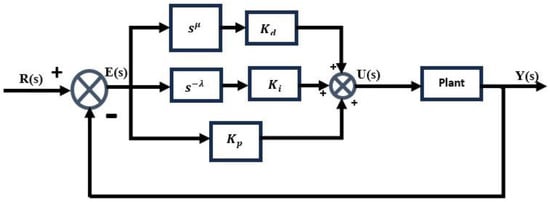
Figure 2.
Block diagram of a general closed-loop system featuring the fractional-order controller.
In this context, represents the controller’s transfer function, whereas and denote the control input and output error signals accordingly. , , and are the proportional, integral, and derivative variables, whereas λ and μ represent the fractional components of the integral and derivative. The fractional-orders λ (fractional integral order) and μ (fractional derivative order) in a Fractional-Order PID (FOPID) controller are typically restricted to the range [0, 2] due to control theory principles and practical considerations. In fractional calculus, λ and μ govern the behavior of integral and derivative terms, and maintaining them within this range ensures the operators remain physically interpretable and aligned with system dynamics. Exceeding this range (λ, μ > 2) can typically lead to instability or impractical responses, as higher orders introduce complex dynamics that are difficult to manage. For level control in spherical tanks, where nonlinear relationships between height and volume are present, fractional orders within [0, 2] provide the flexibility needed for precise tuning while maintaining system stability. This range allows for a broader frequency response, enabling effective handling of slow dynamics and disturbances. Moreover, higher fractional orders add unnecessary complexity to the controller design, complicating real-time computation and offering limited performance benefits. Since spherical tanks typically require moderate control effort, the [0, 2] range balances flexibility and simplicity. Additionally, this restriction ensures compatibility with instrumentation, such as differential pressure transmitters, which may struggle with highly complex dynamics.
Now, recent developments in control design for nonlinear systems have been driven by model-matching methods, notably Approximate Model Matching (AMM), to meet the requirements of a general reference transfer function. The Padé approximation, introduced by Padé in 1890 and widely used for model reduction, compares the time moments and Markov parameters of the plant’s reduced-order model [53]. However, it does not ensure stability for either the reduced model or the closed-loop system. Pal [46] provides a partial solution by introducing a broader set of parameters beyond time moments and Markov parameters. To encompass the full frequency range of interest, one can match the expansion parameters at instead of and , where are chosen to be large or small, real or complex integers. As an outcome, AGTM were introduced in [54,55,56,57,58] as a controller or model design technique across various applications. To identify the optimal expansion points of the AGTM optimization, the Genetic Algorithm (GA) optimization method is employed [47,59] (the reader is referred to [47,59] also for the local minima issue). GA, a stochastic optimization approach inspired by natural selection, was developed by John Holland et al. in 1975 and is based on Darwin’s theory [60]. The main biological processes in GA are crossover, mutation, and selection. The fractional-order controller structure presented in this paper is easy to compute, utilizes output feedback, and results in a low-order controller that is feasible for practical implementation. Thus, the AGTM optimization addresses the fractional-order controller design for nonlinear systems, leveraging these advantages.
4. Approximate Generalized Time Moments (AGTM) Optimization Technique
The AGTM optimization technique aims to determine the parameters of the controller to match the outcome of the reference model and the closed-loop system . The reference model represents the desired time-domain behavior of the closed-loop system. Careful selection of controller parameters is crucial for closely aligning the closed-loop system with the reference model. Imagine a comprehensive format for a general first-order time-delay structure, outlined by the subsequent transfer function,
In the block schematic shown in Figure 3, , and denote the plant, reference model, and the complete closed-loop system, correspondingly. The reference model transfer function is expressed as follows:

Figure 3.
Schematic representation of the AGTM optimization methodology (y is the liquid level, r is its reference value).
Now, the controller parameters must be carefully chosen to ensure the closest possible match between the closed-loop system and the reference model. This can be accomplished by combining several AGTMs and at various extension points, creating a set of linear equations where the unknown features represent the controller parameters. The subsequent transfer function of the closed-loop process turns out to be
In the AGTM optimization-based controller design, the goal is to make sure that the transfer function of the closed-loop system matches the transfer function of the reference model, as shown below:
The times of the closed-loop system are synchronized with those of the reference model at several frequency points , where i = 1, 2, 3 … and represents the number of unknown controller variables that need to be determined by the following:
Using the above equation, we get
to determine the unknown variables of the designed controllers and solve the nonlinear equations in the s-domain using the AGTM optimization method at specified expansion points. The number of unknown variables can be determined by solving the previous nonlinear equation using selected expansion points for . The objective is to optimize the Integral Squared Error (ISE) for maximum similarity between the reference model’s responses and those of the closed-loop system controlled by the designed controller. This optimization problem is usually expressed as find , i = 1, 2, 3 … to reduce the following:
Subject to the constraint that the actual pole components of the closed-loop system must reside on the left half of the s-plane.
Here, represents the response of the closed-loop system with the proposed controller , while denotes the response of the reference model . The controller variables are determined by minimizing the ISE value, achieved by adjusting the initial vector, the expansion points, or both. The ISE criterion focuses on reducing the sum of squared errors over time, placing greater emphasis on larger deviations. This makes it particularly effective in scenarios where minimizing significant errors is critical. Doing so ensures the output remains close to the desired setpoint with minimal overshoot and settling time, which are essential for optimizing system performance and ensuring safety.
Focusing on reducing larger errors enables the controller to swiftly address significant deviations, improving stability and reliability. The ISE approach promotes smoother control actions, which help minimize equipment wear and enhance system stability, particularly when responding to rapid control changes. Additionally, the simple structure of the ISE formula makes it easy to implement, aiding the optimization process in fine-tuning fractional-order controllers, where the inclusion of fractional orders increases the complexity of the parameter space. In the AGTM optimization method, the expansion points are here to find utilize a GA to optimize the ISE performance indices, ensuring a strong alignment between the reference model and the designed responses. The GA operates under the stability constraint specified in Equation (29), enhancing the resilience of the closed-loop system based on the selected expansion points. In particular, the process begins with collecting operational data to train GA to predict or recommend optimal controller parameters based on real-time conditions. AGTM provides an initial set of optimized parameters, which GA refines adaptively to account for changing dynamics and disturbances. This integration allows AGTM to evolve from a static optimization framework into a dynamic, intelligent control methodology, offering real-time adaptability and superior performance in challenging industrial environments. Figure 4a presents a flowchart of the AGTM optimization method for the controller, demonstrating the algorithm’s optimization process. Figure 4b displays, on the other hand, a flowchart of the GA.
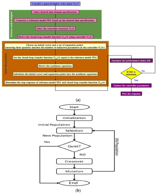
Figure 4.
(a) Flowchart of the AGTM optimization algorithm. (b) Flowchart of the GA optimization algorithm.
Remark 1.
Expansion points can be either positive or negative real numbers or complex points from any quadrant of the s-plane. Typically, the minimum number of expansion points corresponds to the number of unknown controller parameters. When selecting complex points, avoiding conjugate pairs is crucial. These points play a key role in ensuring stability and optimizing closed-loop system performance to meet design specifications [61,62]. Currently, no established theory exists for selecting expansion points that ensure the closed-loop system poles remain in the left half of the s-plane. This study addresses the selection of optimal expansion points for a stable response as a constrained optimization problem, solved using a GA.
Remark 2.
Spherical tanks are particularly challenging to model and control due to nonlinearities, time delays, and uncertainties. These factors, along with parameter variations and disturbances, can degrade control performance, making it difficult to achieve desired outcomes such as settling time, overshoot, and steady-state error using traditional methods. The motivation for using the AGTM optimization method in spherical tank controller design arises from the need for robust solutions to handle the system’s inherent complexities.
5. Simulation and Experimental Results
Multi-model controllers employing the AGTM optimization method were evaluated through simulations and real-time tests across different setpoints to determine their effectiveness in regulating liquid levels. Performance metrics such as tracking accuracy, response time, overshoot, and settling time were analyzed under various conditions. According to the details provided in reference [63], the parameters were assigned the following values: delay time of 20.9 s, rise time of 0.229 s, settling time of 83.5142 s, and a damping ratio of 0.75. Based on these specifications, the transfer function of the reference model is derived and presented as follows:
The GA is employed to identify optimal expansion points using a population size of 100, a crossover fraction of 0.75, an initial population range from 0.1 to 1, and 100 generations. Performance metrics, as defined by Equation (29), quantify the area between the target and designed responses. The goal of minimizing the performance index ISE is to ensure that the designed response closely matches the specified response. The parameters derived for the different controllers are summarized in Table 2.
Table 2.
Simulation results: designed controller variables for the spherical tanks across the entire operating region.
5.1. Simulation Results
The simulation results include 9 cm high step responses of the reference model and various controllers (0–9 cm, 9–18 cm, 18–27 cm, 27–36 cm, and 36–45 cm). Table 3 evaluates the time-domain specifications and performance indices for all controllers using the AGTM optimization method. The results demonstrate that AGTM optimization method-based fractional-order controllers surpass integer-order controllers in terms of rise time, settling time, steady-state error, and peak overshoot while also achieving lower ISE and Integral Absolute Error (IAE) values across all regions. The proposed technique performed a numerical stability analysis of the spherical tank with different controllers, validating findings crucial for practical applications. Additionally, frequency domain response specifications for integer-order and fractional-order controllers are considered, with Table 4 detailing the gain margin, phase margin, gain crossover frequency, and phase crossover. From Table 4, it is evident that AGTM optimization method-based Fractional-Order controllers exhibit higher gain and phase margins, indicating improved system stability.
Table 3.
Simulation results: comparison of time-domain analysis and performance indices for all controllers across different regions.
Table 4.
Simulation results: comparative analysis of frequency responses for all controllers across various regions.
5.2. Comparative Experimental Results
The AGTM-optimized controllers proposed for the spherical tank were tested in real-time across multiple setpoints to assess their effectiveness in controlling liquid levels. Performance metrics, including tracking accuracy, response time, overshoot, and settling time, were evaluated and compared under varying setpoints and disturbances. The new fractional-order control law was also implemented using MATLAB/SIMULINK, employing the FOMCON (Fractional-Order Modeling and Control) toolbox to specify the fractional-order of the integral (λ) and derivative (μ) [64]. The analysis of all controllers involves varying the setpoints, which are selected as 4, 6, 9, 12, 15, 18, 21, 24, 27, 30, 33, 36, 39, 42, and 45 cm. The negative setpoint tracking performance is evaluated across all operational regions. Regarding changes in load, initial setpoints of 6 cm were entered into the system, and corresponding readings were recorded. This process was repeated for setpoints of 9, 15, 18, 24, 27, 33, 36, 39, and 42 cm. At each stage, a sudden disturbance of five liters of water was applied until the system regained stability. Water leakage from the tank was treated as a system error.
5.2.1. Setpoint Variations
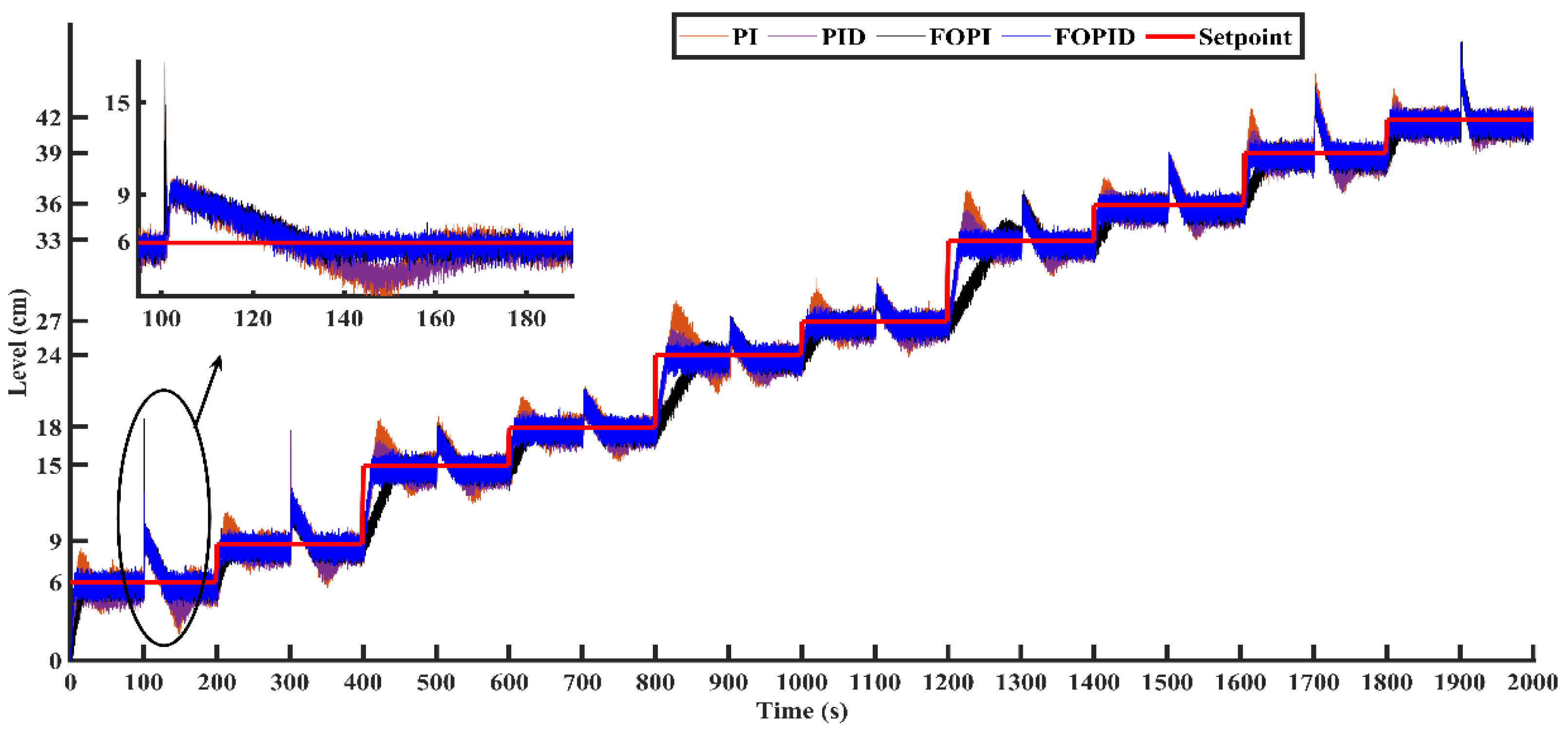
The proposed AGTM optimization technique for different setpoint changes in the spherical tank’s servo response using fractional-order controllers is compared with integer-order controllers, as shown in Figure 5. The results indicate that fractional-order controllers consistently outperform integer-order controllers in both time-domain analysis and performance metrics across all operational regions, as presented in Table 5. As shown in Table 5 and Figure 5, in nonlinear region-1 with a setpoint of 4 cm, the FOPID controller achieves a shorter rise time of 5.936 s, a quicker peak time of 16.3 s, a faster settling time of 18.88 s, a lower peak overshoot of 35.569%, and reduced ISE and IAE values of 0.5532 and 5.3738, respectively. In contrast, the PID controller with the same setpoint has a rise time of 10.968 s, a peak time of 34.136 s, a settling time of 67.132 s, a peak overshoot of 87.5078%, and ISE and IAE values of 1.4606 and 10.2694, respectively. Likewise, in nonlinear region-5 with a setpoint of 45 cm, the FOPID controller shows a lower rise time of 7.26 s, a quicker peak time of 8.15 s, a faster settling time of 12.9 s, a smaller peak overshoot of 3.2933%, and reduced ISE and IAE values of 1.2854 and 7.6545, respectively. In comparison, the PID controller has a rise time of 9.76 s, a peak time of 11.19 s, a settling time of 37.4 s, a peak overshoot of 6.3963%, and ISE and IAE values of 3.1196 and 8.9883, respectively. These performances are reflected consistently across all other regions in both time-domain and performance indices.
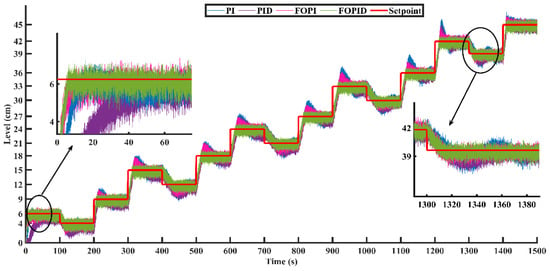
Figure 5.
All Controllers servo response over different regions.
Table 5.
Experimental results: comparison of time-domain analysis and performance indices of all controllers in servo response over different regions of nonlinearity.
Furthermore, the fractional-order controllers’ consistency is observed through the minimal deviation from the desired setpoint value, indicating precise control and accuracy. In every region of operation, the deviation from the setpoint remains minimal, showcasing the controller’s ability to maintain the desired level effectively. Moreover, the fractional-order controllers reach the setpoint much faster compared to integer-order controllers, highlighting their efficiency and quick response to changes. The experimentally modeled spherical tank exhibits stable characteristics across all nonlinear regions.
This stability is crucial as it ensures reliable performance despite the inherent nonlinearity of the system. The spherical tank maintains a steady performance over long durations, proving its robustness and durability in handling various operational conditions. In the extreme nonlinear regions, specifically the lower and uppermost parts of the spherical tank, the ISE and IAE values are significantly low. These low values are indicative of robust controller performance, as they reflect the system’s ability to minimize errors and deviations from the setpoint. The fractional-order controller’s effectiveness in these challenging regions underscores its capability to handle nonlinearity and maintain high performance even under extreme conditions.
5.2.2. Load Variations
The results of fractional-order controllers obtained through the AGTM optimization technique are compared to the ones of integer-order controllers across various operating regions affected by regulatory changes. Figure 6 demonstrates their regulatory performance in the presence of external disturbances represented by a sudden pouring of 5 L of water into the tank. Table 6 presents a comparison of the performance indices for the attained models with the designed controllers, alongside those gathered from previous studies referenced as [1,33].
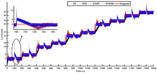
Figure 6.
All Controller regulatory responses under load variations over different regions.
Table 6.
Experimental results: comparison of all controllers in regulatory response under load variations over different regions of nonlinearity.
Based on Table 6 and Figure 6, in nonlinear region-1 with a setpoint of 6 cm, the FOPID controller achieves lower ISE and IAE values of 3.2938 and 13.8307, correspondingly. By contrast, the SIMC-PI [1] controller at the same setpoint has ISE and IAE values of 5134.143 and 2567.652, and the Skogestad’s-PI [33] controller has ISE and IAE values of 5440.887 and 2574.304, respectively.
Similarly, in nonlinear region-5 with a setpoint of 42 cm, the FOPID controller achieves lower ISE and IAE values of 1.5228 and 9.7016, correspondingly. In contrast, the SIMC-PI [1] controller at the same setpoint has ISE and IAE values of 107.6896 and 217.542, and the Skogestad’s-PI [33] controller has ISE and IAE values of 50.12255 and 150.8350, respectively. These performance trends are consistently observed across all other regions in the performance indices.
In conclusion, the proposed AGTM optimization method that uses Fractional-Order controllers shows significantly quicker setpoint tracking compared to integer-order controllers for managing the liquid level in the spherical tank. Moreover, the analysis consistently reduces performance indices across all operating conditions. This indicates that the AGTM optimization technique with Fractional-Order controllers effectively regulates the liquid level with improved efficiency and precision. A closer examination of this table reveals that the ISE and IAE values for regulatory responses in all operational areas are considerably lower in this study than those found in reference [1], which utilized Skogestad’s Internal Model Controller (SIMC) tuning method, and in [33], which employed Skogestad’s tuning approach.
5.3. Single-Model vs. Multi-Model
This section reports in Table 7 and Table 8 data from Table 5 and Table 6 in [47] (with reference to the same experimental setup and same load disturbances) in order to allow the reader to compare them to the results of Table 5 and Table 6 of this paper while thus illustrating how the original multi-modeling approach of this paper improves the very recent single-modeling approach of [47], in almost all the comparable scenarios.
6. Conclusions
This research presents an optimization method for a nonlinear real-time process, specifically spherical tanks, utilizing the AGTM optimization technique to achieve a closed-loop response that mirrors a reference model. The novelty of this study lies in recommending the AGTM optimization algorithm for adjusting the parameters of the multi-model fractional-order controller and assessing the AGTM technique’s performance on spherical tanks. Both simulations and real-time experiments involved developing and applying multi-model fractional-order and integer-order controllers (see also [65,66,67,68]) to control the spherical tank at various setpoints. The load variations exhibit distinct patterns that correspond to different nonlinear regions. Furthermore, the proposed AGTM optimization technique-based fractional-order controllers for different real-time models improve time-domain specifications and provide lower ISE and IAE values compared to the SIMC tuning method and Skogestad’s tuning approach. The experimental results demonstrate the ability of the proposed AGTM optimization technique-based fractional-order controllers to reject load disturbances and maintain robustness against variations in system parameters. Since the described method can be applied to different scenarios, as mentioned in the introduction, the contribution of this paper can be beneficial to both academic and industry practitioners working in various fields, including the mathematical one.
Author Contributions
Conceptualization, N.V.; Methodology, S.J. and N.V.; Software, S.J.; Validation, S.J.; Formal analysis, C.M.V. and N.V.; Investigation, S.J.; Resources, S.J.; Writing—original draft, S.J. and N.V.; Writing—review & editing, C.M.V. All authors have read and agreed to the published version of the manuscript.
Funding
This research received no external funding.
Data Availability Statement
The data will be made available by the authors on request.
Acknowledgments
The authors wish to express their gratitude for the support extended by VIT University during the execution of the measurements.
Conflicts of Interest
The authors declare no conflicts of interest.
References
- Chakravarthi, M.K.; Venkatesan, N. Experimental Validation of a Multi-Model PI Controller for a Non-Linear Hybrid System in LabVIEW. TELKOMNIKA 2015, 13, 547–555. [Google Scholar] [CrossRef]
- Zeigler, J.G.; Nichols, N.B. Optimum settings for automatic controllers. Trans. ASME 1942, 64, 759–768. [Google Scholar] [CrossRef]
- Zhuang, M.; Atherton, D.P. Automatic tuning of optimum PID controllers. Proc. IEEE 1993, 140, 216–224. [Google Scholar] [CrossRef]
- Podlubny, I. Fractional Differential Equations. In Mathematics in Science and Engineering; Academic Press: San Diego, CA, USA, 1999; Volume 198. [Google Scholar]
- Magin, R.L. Fractional Calculus in Bioengineering. Begell House 2004, 32. [Google Scholar] [CrossRef]
- Debnath, L. A brief historical introduction to fractional calculus. Int. J. Math. Educ. Sci. Technol. 2004, 35, 487–501. [Google Scholar] [CrossRef]
- Vinagre, B.M.; Chen, Y.Q. Lecture Notes on Fractional Calculus Applications in Automatic Control and Robotics. In Proceedings of the 41st IEEE CDC2002 Tutorial Workshop, Las Vegas, NV, USA, 10–13 December 2002; pp. 1–310. [Google Scholar]
- Xue, D.; Chen, Y. A comparative introduction of four fractional order controllers. In Proceedings of the 4th IEEE World Congress on Intelligent Control and Automation (WCICA02), Shanghai, China, 10–14 June 2002; pp. 3228–3235. [Google Scholar] [CrossRef]
- Chen, Y. Ubiquitous fractional order controls. In Proceedings of the Second IFAC Symposium on Fractional Derivatives and Applications (IFAC FDA06, Plenary Paper), Porto, Portugal, 19–21 July 2006; pp. 19–21. [Google Scholar] [CrossRef]
- Xue, D.; Zhao, C.; Chen, Y. Fractional order PID control of a DC-motor with an elastic shaft: A case study. In Proceedings of the American Control Conference, Minneapolis, MN, USA, 14–16 June 2006; pp. 3182–3187. [Google Scholar] [CrossRef]
- Manabe, S. The non-integer integral and its application to control systems. Jpn. Inst. Electr. Eng. J. 1960, 80, 589–597. [Google Scholar] [CrossRef]
- Oustaloup, A. Linear feedback control systems of fractional order between 1 and 2. In Proceedings of the IEEE Symposium on Circuit and Systems, Chicago, IL, USA, 27–29 April 1981. [Google Scholar]
- Axtell, M.; Bise, M.E. Fractional calculus applications in control systems. In Proceedings of the IEEE 1990 National Aerospace and Electronics Conference, New York, NY, USA, 21–25 May 1990; pp. 563–566. [Google Scholar] [CrossRef]
- José, A. Tenreiro Machado Analysis and design of fractional-order digital control systems. J. Syst. Anal. Model. Simul. 1997, 27, 107–122. [Google Scholar]
- José, A. Tenreiro Machado Special Issue on Fractional Calculus and Applications. Nonlinear Dyn. 2002, 29, 1–385. [Google Scholar]
- Ortigueira, M.D.; Machado, J.A.T. Special Issue on Fractional Signal Processing and Applications. Signal Process. 2003, 83, 2285–2480. [Google Scholar] [CrossRef]
- Ashwini, A.; Sriram, S.R.; Joel Livin, A. Quadruple spherical tank systems with automatic level control applications using fuzzy deep neural sliding mode FOPID controller. J. Eng. Res. 2023. [Google Scholar] [CrossRef]
- Jegatheesha, A.; Agees Kumar, C. Novel fuzzy fractional order PID controller for nonlinear interacting coupled spherical tank system for level process. Microprocess. Microsyst. 2020, 72, 102948. [Google Scholar] [CrossRef]
- Arivalahan, R.; Tamilarasan, P.; Kamalakannan, M. Liquid level control in two tanks spherical interacting system with fractional order proportional integral derivative controller using hybrid technique: A hybrid technique. Adv. Eng. Softw. 2023, 175, 103316. [Google Scholar] [CrossRef]
- Debnath, B.; Mija, S.J. Emotional Learning Based Controller for Quadruple Tank System—An Improved Stimuli Design for Multiple Set-Point Tracking. IEEE Trans. Ind. Electron. 2021, 68, 11296–11308. [Google Scholar] [CrossRef]
- Jáuregui, C.; Duarte, M.A.; Oróstica, R.; Travieso, J.C.; Beytía, O. Conical Tank Level Control with Fractional PID. IEEE Lat. Am. Trans. 2016, 14, 2598–2604. [Google Scholar] [CrossRef]
- Meng, X.; Yu, H.; Zhang, J.; Xu, T.; Wu, H.; Yan, K. Disturbance Observer-Based Feedback Linearization Control for a Quadruple-Tank Liquid Level System. ISA Trans. 2022, 122, 146–162. [Google Scholar] [CrossRef] [PubMed]
- Huo, M.; Luo, H.; Wang, X.; Yang, Z.; Kaynak, O. Real-Time Implementation of Plug-and-Play Process Monitoring and Control on an Experimental Three-Tank System. IEEE Trans. Ind. Inform. 2021, 17, 6448–6456. [Google Scholar] [CrossRef]
- Das, D.; Chakraborty, S.; Mehta, U.; Raja, L.G. Fractional Dual-Tilt Control Scheme for Integrating Time Delay Processes: Studied on a Two-Tank Level System. IEEE Access 2024, 12, 7479–7489. [Google Scholar] [CrossRef]
- Xu, T.; Yu, H.; Yu, J.; Meng, X. Adaptive Disturbance Attenuation Control of Two Tank Liquid Level System With Uncertain Parameters Based on Port-Controlled Hamiltonian. IEEE Access 2020, 8, 47384–47392. [Google Scholar] [CrossRef]
- Fu, Y.; Du, Q.; Zhou, X.J.; Fu, J.; Chai, T.Y. Dual-Rate Adaptive Decoupling Controller and Its Application to a Dual-Tank Water System. IEEE Trans. Control Syst. Technol. 2020, 28, 2515–2522. [Google Scholar] [CrossRef]
- Bhookya, J.; Kumar, V.M.; Ravi Kumar, J.; Seshagiri, R. A Implementation of PID controller for liquid level system using mGWO and integration of IoT application. J. Ind. Inf. Integr. 2022, 28, 100368. [Google Scholar] [CrossRef]
- Reddy, S.A.; Reddy, N.G. An adaptive fractional order controller design: A realization for liquid level regulation in liquid level plant. Meas. Sens. 2024, 31, 100977. [Google Scholar] [CrossRef]
- Wang, G.; Jia, Q.-S.; Qiao, J.; Bi, J.; Zhou, M. Deep Learning-Based Model Predictive Control for Continuous Stirred-Tank Reactor System. IEEE Trans. Neural Netw. Learn. Syst. 2021, 32, 3643–3652. [Google Scholar] [CrossRef]
- Matušů, R.; Şenol, B.; Pekař, L. Robust PI Control of Interval Plants With Gain and Phase Margin Specifications: Application to a Continuous Stirred Tank Reactor. IEEE Access 2020, 8, 145372–145380. [Google Scholar] [CrossRef]
- Alshammari, O.; Mahyuddin, M.N.; Jerbi, H. An Advanced PID Based Control Technique With Adaptive Parameter Scheduling for A Nonlinear CSTR Plant. IEEE Access 2019, 7, 158085–158094. [Google Scholar] [CrossRef]
- Chakravarthi, K.M.; Venkatesan, N. Design and Implementation of Adaptive Model Based Gain Scheduled Controller for a Real-Time Nonlinear System in LabVIEW. Res. J. Appl. Sci. Eng. Technol. 2015, 10, 188–196. [Google Scholar] [CrossRef]
- Joshi, S.M.; Tao, G.; Patre, P. Direct adaptive control using an adaptive reference model. Int. J. Control 2011, 84, 180196. [Google Scholar] [CrossRef]
- Bentayeb, A.; Maamri, N.; Trigeassou, J.-C. Design of PID controllers for delayed MIMO plants using the moments-based approach. J. Electr. Eng. 2006, 57, 318–328. [Google Scholar]
- Damodaran, S.; Kumar, T.S.; Sudheer, A.P. Design and implementation of GA tuned PID controller for desired interaction and trajectory tracking of a wheeled mobile robot. In Proceedings of the 2017 3rd International Conference on Advances in Robotics, New Delhi, India, 28 June–2 July 2017. [Google Scholar] [CrossRef]
- Yakoub, Z.; Chetoui, M.; Amairi, M.; Aoun, M. Model-based fractional order controller design. IFAC-Pap. 2017, 50, 1043110436. [Google Scholar] [CrossRef]
- Quinn, S.B.; Sanathanan, C.K. Model matching control for multivariable systems I. Stable plants. J. Frankl. Inst. 1990, 327, 699712. [Google Scholar] [CrossRef]
- Quinn, S.B.; Sanathanan, C.K. Model matching control for multivariable systems II. Unstable plants. J. Frankl. Inst. 1990, 327, 713729. [Google Scholar] [CrossRef]
- Szita, G.; Sanathanan, C.K. A model matching approach for designing decentralized MIMO controllers. J. Frankl. Inst. 2000, 337, 641660. [Google Scholar] [CrossRef]
- Szita, G.; Sanathanan, C.K. Model matching controller design for disturbance rejection. J. Frankl. Inst. 1996, 333, 747772. [Google Scholar] [CrossRef]
- Das, S.K.; Pota, H.R.; Petersen, I.R. Multivariable negative imaginary controller design for damping and cross-coupling reduction of nanopositioners: A reference model matching approach. IEEE/ASME Trans. Mechatron. 2015, 20, 31233134. [Google Scholar] [CrossRef]
- Mittal, S.K.; Chandra, D.; Dwivedi, B. The effects of time moments and Markov-parameters on reduced-order modeling. ARPN J. Eng. Appl. Sci. 2009, 4, 8–14. [Google Scholar]
- Dey, S.; Kumar, T.S.; Ashok, S.; Shome, S.K. Robust cascade control strategy for trajectory tracking to decouple disturbances using 3-degree-of-freedom inertial stabilized platform and its experimental validation. Trans. Inst. Meas. Control. 2023, 20, 01423312221150290. [Google Scholar] [CrossRef]
- Jayaram, S.; Venkatesan, N. Research on Fractional-Order Controllers for Liquid Level Control of Nonlinear System Using Optimization Technique. In Proceedings of the IEEE 9th International Conference on Control, Decision and Information Technologies (CoDIT), Rome, Italy, 3–6 July 2023; pp. 403–408. [Google Scholar] [CrossRef]
- Pal, J. An algorithm method for the simplification of linear dynamic scalar systems. Int. J. Control 1986, 43, 257–269. [Google Scholar] [CrossRef]
- Beevi, F.P.; Kumar, T.S.; Jacob, J. Two degree of freedom controller design by AGTM/AGMP matching method for time delay systems. Procedia Technol. 2016, 25, 20–27. [Google Scholar] [CrossRef]
- Jayaram, S.; Venkatesan, N. Design and implementation of the fractional-order controllers for a real-time nonlinear process using the AGTM optimization technique. Sci. Rep. 2024, 14, 31714. [Google Scholar] [CrossRef]
- Sundaresan, K.R.; Krishnaswamy, P.R. Estimation of time delay time constant parameters in time, frequency, and Laplace domains. Can. J. Chem. Eng. 1978, 56, 257–262. [Google Scholar] [CrossRef]
- Li, G.; Zhang, Y.; Guan, Y.; Li, W. Stability analysis of multi-point boundary conditions for fractional differential equation with non-instantaneous integral impulse. Math. Biosci. Eng. 2023, 20, 7020–7041. [Google Scholar] [CrossRef] [PubMed]
- Fan, H.; Tang, J.; Shi, K.; Zhao, Y. Hybrid Impulsive Feedback Control for Drive–Response Synchronization of Fractional-Order Multi-Link Memristive Neural Networks with Multi-Delays. Fractal Fract. 2023, 7, 495. [Google Scholar] [CrossRef]
- Fan, H.; Rao, Y.; Shi, K.; Wen, H. Global Synchronization of Fractional-Order Multi-Delay Coupled Neural Networks with Multi-Link Complicated Structures via Hybrid Impulsive Control. Mathematics 2023, 11, 3051. [Google Scholar] [CrossRef]
- Podlubny, I. Fractional-Order Systems and Fractional-Order Controllers; Institute of Experimental Physics, Slovak Academy of Sciences: Kosice, Slovakia, 1994. [Google Scholar]
- Baker, G. A Essentials of Pade Approximation; Academic Press: New York, NY, USA, 1975. [Google Scholar]
- Kumar, T.S. Model Matching Controller Design Methods with Applications in Electrical Power Systems. Ph.D. Thesis, IIT Kharagpur, Kharagpur, India, 2009. [Google Scholar]
- Muthukumari, S.; Kanagalakshmi, S.; Kumar, T.S. Centralized model matching integer/fractional-order controller design for multivariable processes with real-time validation. Trans. Inst. Meas. Control 2023, 46, 1828–1841. [Google Scholar] [CrossRef]
- Damodaran, S.; Kumar, T.S.; Sudheer, A.P. Generalized method for rational approximation of SISO/MIMO fractional-order systems using squared magnitude function. Trans. Inst. Meas. Control 2023, 46, 207–222. [Google Scholar] [CrossRef]
- Muthukumari, S.; Kanagalakshmi, S.; Kumar, T.S. Development of a novel model matching decentralized controller design algorithm and its experimental validation through load frequency controller implementation in restructured power system using TMS320F28379D control CARD. ISA Trans. 2024, 148, 285–306. [Google Scholar] [CrossRef]
- Beevi, F.P.; Kumar, T.S.; Jacob, J.; Beevi, D.P. Novel two degree of freedom model matching controller for set-point tracking in MIMO systems. Comput. Electr. Eng. 2017, 61, 1–14. [Google Scholar] [CrossRef]
- Muhammed, S.; Mahesh, P.V.; Mathew, A.T.; Kumar, T.S. Model Approximation and Controller Synthesis for H∞ Robust Control of Multiple Time Delay Transfer Functions. Int. Rev. Autom. Control. (IREACO) 2016, 9, 1–10. [Google Scholar] [CrossRef]
- Holland, J. Adaptation in Natural and Artificial Systems: An Introductory Analysis with Applications to Biology, Control, and Artificial Intelligence; University of Michigan Press: Ann Arbor, MI, USA, 1975. [Google Scholar]
- Priyanka, K.K.D.; Santhosh Kiran, M.; Rajarao, G. A New Approach for Design of Model Matching Controllers for Time Delay Systems by Using GA Technique. Int. J. Eng. Res. Appl. 2015, 5, 89–99. [Google Scholar]
- Ganguli, S.; Kaur, G.; Sarkar, P. An approximate model matching technique for controller design of linear time-invariant systems using hybrid firefly-based algorithms. ISA Trans. 2022, 127, 437–448. [Google Scholar] [CrossRef]
- Norman, S. Nise Control Systems Engineering, 6th ed.; Wiley India Private Ltd.: New Delhi, India, 2018. [Google Scholar]
- Tepljakov, A.; Petlenkov, E.; Belikov, J. FOMCON: A MATLAB toolbox for fractional-order system identification and control. Int. J. Microelectron. Comput. Sci. 2011, 2, 51–62. [Google Scholar]
- Padula, F.; Visioli, A. Tuning rules for optimal PID and fractional-order PID controllers. J. Process Control 2011, 21, 69–81. [Google Scholar] [CrossRef]
- Vu, T.N.L.; Lee, M. Analytical design of fractional-order proportional-integral controllers for time-delay processes. ISA Trans. 2013, 52, 583–591. [Google Scholar] [CrossRef] [PubMed]
- Roy, P.; Roy, B.K. Fractional order PI control applied to level control in coupled two tank MIMO system with experimental validation. Control Eng. Pract. 2016, 48, 119–135. [Google Scholar] [CrossRef]
- Vinopraba, T.; Sivakumaran, N.; Narayanan, S.; Radhakrishnan, T.K. Design of internal model control based fractional order PID controller. J. Control Theory Appl. 2012, 10, 297–302. [Google Scholar] [CrossRef]


Disclaimer/Publisher’s Note: The statements, opinions and data contained in all publications are solely those of the individual author(s) and contributor(s) and not of MDPI and/or the editor(s). MDPI and/or the editor(s) disclaim responsibility for any injury to people or property resulting from any ideas, methods, instructions or products referred to in the content. |
© 2025 by the authors. Licensee MDPI, Basel, Switzerland. This article is an open access article distributed under the terms and conditions of the Creative Commons Attribution (CC BY) license (https://creativecommons.org/licenses/by/4.0/).