Curvature Control for Plane Curves

Abstract

We define a family of special functions (the CSI ones), which can be used to write any parameterized plane curve with polynomial curvature explicitly. These special functions generalize the Fresnel integrals, and may have an interest in their own right. We prove that any plane curve with polynomial curvature is asymptotically a pseudo-spiral. Using the CSI functions, we can approximate, locally, any plane curve; this approach provides a useful criterion for a (local) classification of plane curves. In addition, we present a new algorithm for finding an arc-length parametrization for any curve, within a prescribed degree of approximation.

1. Introduction

Smooth plane curves are fundamental objects in mathematics, and are of both theoretical interest and practical importance for applications in computer graphics, engineering, and physics. Understanding them is crucial for analyzing shapes and motion in a planar context. The study of plane curves has a rich history, with contributions from renowned mathematicians. Over time, the theory of these curves has evolved, leading to a deeper understanding of their properties and behaviors [1,2,3,4,5].

One of the main problems in the modern theory of plane curves is how to “control” them through their curvature. Curvature control involves manipulating and analyzing the curvature properties of curves, which have significant implications for both theoretical research and practical applications. By controlling curvature, one can design curves with specific properties, optimize shapes, and solve complex geometric problems. Curvature control has practical applications, such as in the automotive industry for designing aerodynamic car bodies and in computer graphics for creating realistic animations [6,7,8,9,10,11,12].

A classical result in early differential geometry states that a plane regular curve is completely determined by its curvature function, modulo an orientation-preserving parameter change and a proper isometry of the plane. Due to the huge diversity of (smooth) real valued functions on (intervals of) the real line, there is no hope to classify (even locally) the plane curves by a tractable system of invariants based on arbitrary (curvature) functions.

For many applications, approximate solutions are sufficient, so we may attempt to approximate the plane curves with “simpler” and classifiable ones [13]. The first idea which comes to mind is to approximate a plane curve $c(t)=(x(t),y(t))$ by the family of curves

$$(TA{Y}_{m}x(t),TA{Y}_{n}y(t)),$$

where $TA{Y}_{m}x(t)$ and $TA{Y}_{n}y(t)$ are the polynomial functions of degree m and n from the Taylor developments of x and y, respectively. In this paper, we adopt another approach: we consider the Taylor polynomials $TA{Y}_{n}K$ of the curvature function K of the curve c and we associate the (unique, modulo some restrictions) plane curves with these curvature functions. This approximation of the initial curve c by the new family of curves (with polynomial curvature) has two advantages: it involves only one family of Taylor polynomials (and remainders, error evaluations, arc-length parametrization [14,15], etc.), and we deal with simpler curvature functions with respect to the first method.

1.1. Short Historical Notes

Curve control through curvature is a classical topic that has gained renewed interest due to modern applications [6,7,10,12,16]. In particular, the spirals and their generalizations are of special importance [17,18].

The Cornu spiral [17] distinguishes itself by having linear curvature function. There are several generalizations of the Cornu spiral in [13,19,20,21,22], including one in the present paper. In particular, the pseudo-spirals of Pirondini [23] suggest how to lay the groundwork for approximation of all plane curves with polynomial curvature.

There are several papers with approximations of plane curves, from different points of view. We quote but a few: [8,9,13].

1.2. Our Contribution

The main focus of our paper is the curvature control of plane curves, through an easily classifiable family of “the simplest possible” but, at the same time, “general enough” plane curves.

In Section 2, we recall three examples, with detailed calculations, of a logarithmic spiral, a Cornu spiral, and a catenary curve. These curves have in common the type of the curvature function (a rational function) and the property that they can derive from the curvature, directly, by integration. Unfortunately, these are exceptions, not the rule.

In Section 3, we build the main tool: the special functions of CSI-type. Using them, we define the CS-curves, which serve as building blocks for a deeper understanding of all plane curves with polynomial curvature (Theorem 1). The latter are fully characterized in Proposition 2. We prove that, asymptotically, the plane curves with polynomial curvature are pseudo-spirals (Theorem 2).

In Section 4, we give an (approximate) classification of plane curves, as limits of plane curves with polynomial curvature functions.

As a by-product, we provide a simple algorithm for obtaining the arc-length parametrization for any plane curve, within a prescribed degree of approximation. This procedure is a new one (to our knowledge), and provides a solution to a difficult (and poorly represented in the literature) problem of plane curve applications.

1.3. Conventions

If not otherwise stated, we denote by I an interval of $\mathbb{R}$, containing 0; the plane curves $c:I\to {\mathbb{R}}^2$ have I the maximal definition domain; and all curves are supposed smooth, even if most results are still valid under much weaker hypotheses. Whenever necessary, the curves will be “pinned” through the conditions $c(0)=(0,0)$ and $\dot{c}(0)=(1,0)$.

2. Ad Hoc Examples to Point out the Path

One knows that a plane curve with constant curvature function K is (part of) a line, if $K=0$, or (an arc of) a circle of radius ${\displaystyle \frac{1}{\mid K\mid }}$, otherwise. As soon as the curvature function ceases to be trivial, determining the curve becomes problematic. We show this through three simple examples.

Proposition 1.

Let $X=X(s)$ be an arc-length parameterized plane curve, K its curvature function, and “a” a fixed non-null real constant.

(i) If $K(s)={\displaystyle \frac{1}{a·s}}$, then X is a logarithmic spiral.

(ii) If $K(s)=s$, then X is an Euler (also known as Cornu) spiral.

(iii) If $K(s)={\displaystyle \frac{a}{s^2+a^2}}$, then X is a catenary curve.

Proof. 

Denote by $\theta =\theta (s)$ the slope of the tangent to the curve, and by ${\theta }^{\prime }$ its derivative with respect to the parameter s. Then,

$$T(s)=(cos\theta (s),sin\theta (s)),N(s)=(-sin\theta (s),cos\theta (s))$$

and ${\theta }^{\prime }(s)=K(s)$.

(i) From the hypothesis, we deduce that

$${\theta }^{\prime }(s)={\displaystyle \frac{1}{a·s}}.$$

The solution of this ODE is

$$\theta (s)=ln(A·s^{{\displaystyle \frac{1}{a}}}),$$

(1)

where A is a positive integration constant. Equation (1) rewrites, in an equivalent form, as

$$s=A^{-a}·exp(a·\theta (s)).$$

From

$${\displaystyle \frac{dX}{ds}}=T(s),$$

we obtain, by integration, that

$$X(s)={\displaystyle \frac{a^{2}s}{a^2+1}}\left({\displaystyle \frac{1}{a}}sin(ln(A{s}^{{\displaystyle \frac{1}{a}}}))+cos(ln(A{s}^{{\displaystyle \frac{1}{a}}})),sin(ln(A{s}^{{\displaystyle \frac{1}{a}}}))-{\displaystyle \frac{1}{a}}cos(ln(A{s}^{{\displaystyle \frac{1}{a}}}))\right).$$

(2)

The curve X is a logarithmic spiral. We remark on its atypical parametrization (due to arc-length). Any other solution can be obtained from X, by an orientation-preserving parameter change, and/or by a proper isometry of the plane.

(ii) From the hypothesis, we deduce that ${\theta }^{\prime }(s)=s$. The solution of this ODE is

$$\theta (s)={\displaystyle \frac{s^2}{2}}+B,$$

(3)

where B is an integration constant. From Equation (3), we obtain

$$X(s)=\left(\int cos({\displaystyle \frac{s^2}{2}}+B)ds,\int sin({\displaystyle \frac{s^2}{2}}+B)ds\right).$$

(4)

Denote

$$I_1(s):=\int cos({\displaystyle \frac{s^2}{2}}+B)ds,I_2(s):=\int sin({\displaystyle \frac{s^2}{2}}+B)ds.$$

We rewrite this, in an equivalent form, as

$$I_1(s)=cosB·\int cos({\displaystyle \frac{s^2}{2}})ds-sinB·\int sin({\displaystyle \frac{s^2}{2}})ds,$$

$$I_2(s)=cosB·\int sin({\displaystyle \frac{s^2}{2}})ds+sinB·\int cos({\displaystyle \frac{s^2}{2}})ds.$$

If we use Maclaurin series expansion, there exist two integration constants, D and E, such that

$$I_1(s)=cosB·\sum _{n=0}^{\infty }{\displaystyle \frac{{(-1)}^n·s^{4n+1}}{2^{2n}·(2n)!(4n+1)}}-sinB·\sum _{n=0}^{\infty }{\displaystyle \frac{{(-1)}^n·s^{4n+3}}{2^{2n+1}·(2n+1)!(4n+3)}}+D,$$

$$I_2(s)=cosB·\sum _{n=0}^{\infty }{\displaystyle \frac{{(-1)}^n·s^{4n+3}}{2^{2n+1}·(2n+1)!(4n+3)}}+sinB·\sum _{n=0}^{\infty }{\displaystyle \frac{{(-1)}^n·s^{4n+1}}{2^{2n}·(2n)!(4n+1)}}+E.$$

We obtain a family of Cornu spirals,

$$X(s)=\left(I_1(s),I_2(s)\right),$$

(5)

depending on the three constants (B, D, and E).

We remark that the integrals $I_1$ and $I_2$ are related to the Fresnel integrals,

$$C(t):={\int }_0^{t}cos(s^2)ds,S(t):={\int }_0^{t}sin(s^2)ds$$

respectively.

(iii) From the hypothesis, we deduce

$${\theta }^{\prime }(s)={\displaystyle \frac{a}{s^2+a^2}}.$$

The solution of this ODE is

$$\theta (s)=arctan({\displaystyle \frac{s}{a}})+c,$$

(6)

where c is an integration constant. From formula (6), we obtain

$$X(s)=\left(\int cos(arctan({\displaystyle \frac{s}{a}})+c)ds,\int sin(arctan({\displaystyle \frac{s}{a}})+c)ds\right).$$

(7)

Denote

$$I_1(s):=\int cos(arctan({\displaystyle \frac{s}{a}})+c)ds,I_2(s):=\int sin(arctan({\displaystyle \frac{s}{a}})+c)ds.$$

We rewrite it, in an equivalent form, as

$$I_1(s)=cosc·\int cos(arctan({\displaystyle \frac{s}{a}}))ds-sinc·\int sin(arctan({\displaystyle \frac{s}{a}}))ds,$$

$$I_2(s)=cosc·\int sin(arctan({\displaystyle \frac{s}{a}}))ds+sinc·\int cos(arctan({\displaystyle \frac{s}{a}}))ds.$$

We calculate, by integration (and neglecting the two integration constants), that

$$I_1(s)=(cosc)·a·arcsinh({\displaystyle \frac{s}{a}})-(sinc)·\sqrt{s^2+a^2},$$

$$I_2(s)=(cosc)·\sqrt{s^2+a^2}+(sinc)·a·arcsinh({\displaystyle \frac{s}{a}}).$$

We obtain the catenary curve,

$$X(s)=\left(I_1(s),I_2(s)\right).$$

(8)

 □

Remark 1.

(i) (Generalization) The problem of finding the arc-length parameterized plane curves of a prescribed (smooth) curvature function K reduces to the determination of the (well-known [6]) family,

$$X(s)=\left(\int cos(\int K(s)ds)ds,\int sin(\int K(s)ds)ds\right),$$

(9)

which depends on three real (integration) parameters. One can obtain the explicit X, whenever we are able to integrate by quadratures the three indefinite integrals.

For example, when K is a polynomial function, it follows that its indefinite integral is also a polynomial function. This is the easy step. The hard step is the calculation the cosine or the sine of a polynomial function.

(ii) The three constants which appear when integrating (9) determine the translation and the rotation parameters, as “degrees of freedom”. In order to canonically fix (the “initial position” of) such a curve, we shall implicitly suppose $X(0)=(0,0)$ and $\theta (0)=0$.

3. Plane Curves with Polynomial Curvature Function

Definition 1.

Let $f=a_m{X}^m+\dots +a_{1}X+a_0$ a fixed polynomial in $\mathbb{R}[X]$ of degree m. The special function

$$c{i}_f(t):={\int }_0^{t}cos(a_m{s}^m)\cdots cos(a_0{s}^0)ds$$

is called the f-cosine integral (f-CI for short).

In a similar way, we define the f-sine integral (f-SI for short),

$$s{i}_f(t):={\int }_0^{t}sin(a_m{s}^m)\cdots sin(a_0{s}^0)ds$$

Consider another fixed polynomial $h=b_n{X}^n+\dots +b_{1}X+b_0$ in $\mathbb{R}[X]$ of degree n. The special function

$$cs{i}_{f,h}(t):={\int }_0^{t}cos(a_m{s}^m)\cdots cos(a_0{s}^0)·sin(b_n{s}^n)\cdots sin(b_0{s}^0)ds$$

(10)

is called the $(f,h)$-cossine integral ($(f,h)$-CSI for short).

Remark 2.

(i) Obviously, the sets of the CIs, SIs and CSIs are in one-to-one correspondence with the sets $\mathbb{R}[X]$, $\mathbb{R}[X]$ and $\mathbb{R}[X]\times \mathbb{R}[X]$, respectively.

(ii) If $h={\displaystyle \frac{\pi }{2}}$, then $cs{i}_{f,h}=c{i}_f$.

(iii) If $f=0$, then $cs{i}_{f,h}=s{i}_h$.

(iv) We point out some particular cases of f-CIs: (iv)₁ $f=a_0$, $c{i}_f(t)=cos(a_0)·t$; (iv)₂ $f=a_{1}X+a_0$, $c{i}_f(t)={\displaystyle \frac{1}{a_1}}·sin(a_{1}t)·cos(a_0)$.

Similar examples can be easily constructed for f-SIs, but we skip them.

(v) Consider the polynomial $f=a_2{X}^2+a_{1}X+a_0$, and

$$\begin{array}{l}c{i}_f(t)=\sqrt{{\displaystyle \frac{\pi }{8a_2}}}\{cos({\displaystyle \frac{a_1^2}{4a_2}})[C({\displaystyle \frac{2a_{2}t-a_1}{\sqrt{2\pi a_2}}})+C({\displaystyle \frac{2a_{2}t+a_1}{\sqrt{2\pi a_2}}})]+\\ +sin({\displaystyle \frac{a_1^2}{4a_2}})[S({\displaystyle \frac{2a_{2}t-a_1}{\sqrt{2\pi a_2}}})+S({\displaystyle \frac{2a_{2}t+a_1}{\sqrt{2\pi a_2}}})]\}·cos(a_0),\end{array}$$

where C and S are the Fresnel integrals. This function appears in the definition of the clothoid.

(vi) For $n\ge 1$ a natural number, consider

$${\int }_0^{t}cos(s^n)ds,{\int }_0^{t}sin(s^n)ds.$$

These CIs and SIs are involved in the definition of the pseudo-spirals of Pirondini.

Definition 2.

A plane curve is (parameterized as) a cossine curve (CS-curve or CSC, for short) if each of its components is a linear combination of CSI special functions. As particular cases, we define similarly the cosine curve (C-curve or CC for short) and the sine curve (S-curve or SC for short).

Remark 3.

The general form for a CS curve is

$$c(t)=\left(\sum _{i=1}^k{A}_i·cs{i}_{f_i,h_i}(t),\sum _{j=1}^l{B}_j·cs{i}_{{\tilde{f}}_j,{\tilde{h}}_j}(t)\right),$$

where $A_1$, …, $A_k$, $B_1$, …, $B_l$ are (arbitrary) real constants; $f_1$, …, $f_k$, ${\tilde{f}}_1$, …, ${\tilde{f}}_l$, $h_1$, …, $h_k$, and ${\tilde{h}}_1$, …, ${\tilde{h}}_l$ are (arbitrary) polynomials.

The general forms of CCs and of SCs can be written in similar formulas.

Examples. (i) The lines admit parametrizations as C-curves. For example, the curve $c(t)=(tcos(0),tcos(\pi ))$ provides a parametrization of the second bisector line of the canonical coordinate frame.

(ii) The circles admit parametrizations as CSI-curves. For example, the (translated by (1,0)) unit circle has the parametrization $c(t)=({\int }_0^{t}sin(s)ds,{\int }_0^{t}cos(s)ds)$.

(iii) Both previous curves have, obviously, polynomial curvature functions. There exist C-curves without polynomial curvature function, too. For example,

$$c(t)=({\int }_0^{t}cos(s^2)ds,{\int }_0^{t}cos(s)ds),$$

whose image can be seen in Figure 1. The curvature function is

$$K(t)=(2tcostsin{t}^2-cos{t}^{2}sint)·{(co{s}^{2}t+co{s}^2{t}^2)}^{-{\displaystyle \frac{3}{2}}}.$$

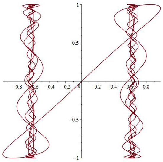
Figure 1. Picture of the parametric curve in Example (iii), for $t\in [-20,20]$.

(iv) We slightly modify the previous example, by introducing a sum of CIs on the first component. The new C-curve,

$$c(t)=({\int }_0^t[cos(s^2)+cos(s)]ds,{\int }_0^{t}cos(s)ds)$$

changes its form as in Figure 2.

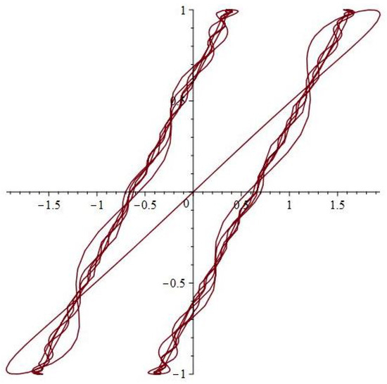
Figure 2. Picture of the parametric curve in Example (iv), for $t\in [-20,20]$.

The curvature function

$$K(t)=[2tcostsin{t}^2-sintcos{t}^2]·{[co{s}^{2}t+{(cos{t}^2+cost)}^2]}^{-{\displaystyle \frac{3}{2}}}$$

does not have a polynomial form.

(v) Other examples of CSCs are the clothoid (also known as the Cornu spiral or Euler spiral; see Figure 3),

$$c(t)=({\int }_0^{t}cos(s^2)ds,{\int }_0^{t}sin(s^2)ds)$$

and the pseudo-spiral (see Figure 4 and Figure 5),

$$c(t)=({\int }_0^{t}cos(s^n)ds,{\int }_0^{t}sin(s^n)ds)$$

(which generalizes the preceding one).

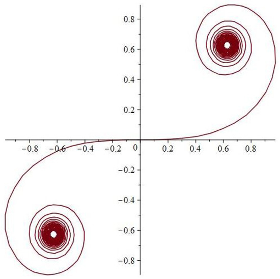
Figure 3. Picture of the clothoid for $t\in [-20,20]$.

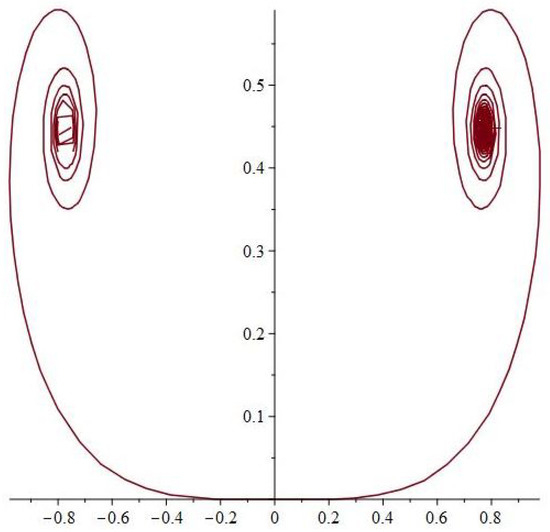
Figure 4. Picture of the pseudo-spiral for $t\in [-5,12]$ and n = 3.

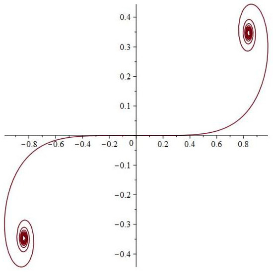
Figure 5. Picture of the pseudo-spiral for $t\in [-3,3]$ and n = 4.

The first step toward the classification result of the plane curves is the following.

Theorem 1.

If an arc-length parameterized plane curve has polynomial curvature function K, then it is a CS curve.

Proof. 

Since K is a polynomial function, then any of its indefinite integrals $\theta$ is also a polynomial function. We reduced the problem to show that an indefinite integral of the cosine and of the sine, composed with a polynomial function, can be written as a linear combination of $CSI$s.

The elementary formulas are

$$\begin{array}{c}cos(a_n{s}^n+\dots a_{1}s+a_0)=cos(a_n{s}^n+\dots a_{1}s)cos(a_0)-sin(a_n{s}^n+\dots a_{1}s)sin(a_0)=\\ =[cos(a_n{s}^n+\dots a_2{s}^2)cos(a_{1}s)-sin(a_n{s}^n+\dots a_2{s}^2)sin(a_{1}s)]cos(a_0)-\\ -[cos(a_n{s}^n+\dots a_2{s}^2)sin(a_{1}s)+sin(a_n{s}^n+\dots a_2{s}^2)cos(a_{1}s)]sin(a_0).\end{array}$$

We repeat the calculations by replacing $cos(a_n{s}^n+\dots a_2{s}^2)$ and $sin(a_n{s}^n+\dots a_2{s}^2)$ with sums of products of cosines and sines applied to polynomial functions with one-less terms. In a finite number of steps, we obtain a linear combination of products of cosines and sines, applied to monomials only. □

Remark 4.

The proof of the previous theorem is a mixture of qualitative arguments and of some calculus. There was no reason to give more detail. However, in some applications we may need a more precise explicit formula for (the general form of) an arc-length parameterized curve with polynomial curvature function.

The next formula for the sine of an arbitrary sum is known [24]:

$$sin({\alpha }_1+\dots +{\alpha }_m)=\sum _{k=0}^{\left[{\displaystyle \frac{m-1}{2}}\right]}\sum _{\begin{array}{c}A\subseteq \{1,\dots ,m\}\\ \mid A\mid =2k+1\end{array}}{(-1)}^k\prod _{i\in A^C}cos({\alpha }_i)\prod _{j\in A}sin({\alpha }_j).$$

(11)

We give here a sketch proof for it and for the cosine analogue,

$$cos({\alpha }_1+\dots +{\alpha }_m)=\sum _{k=0}^{\left[{\displaystyle \frac{m}{2}}\right]}\sum _{\begin{array}{c}A\subseteq \{1,\dots ,m\}\\ \mid A\mid =2k\end{array}}{(-1)}^k\prod _{i\in A^C}cos({\alpha }_i)\prod _{j\in A}sin({\alpha }_j).$$

(12)

Indeed, we write

$$e^{i({\alpha }_1+\dots +{\alpha }_m)}=[cos({\alpha }_1)+isin({\alpha }_1]\dots [cos({\alpha }_m)+isin({\alpha }_m].$$

The Formulas (11) and (12) follow from

$$sin({\alpha }_1+\dots +{\alpha }_m)=Im{e}^{i({\alpha }_1+\dots +{\alpha }_m)},cos({\alpha }_1+\dots +{\alpha }_m)=Re{e}^{i({\alpha }_1+\dots +{\alpha }_m)}$$

and a careful combinatorial calculation.

For example, when $m=3$ and $m=4$, respectively, Formula (12) gives:

$$\begin{array}{c}cos({\alpha }_1+{\alpha }_2+{\alpha }_3)=cos({\alpha }_1)cos({\alpha }_2)cos({\alpha }_3)-cos({\alpha }_1)sin({\alpha }_2)sin({\alpha }_3)-\\ -cos({\alpha }_2)sin({\alpha }_1)sin({\alpha }_3)-cos({\alpha }_3)sin({\alpha }_1)sin({\alpha }_2),\end{array}$$

$$\begin{array}{c}cos({\alpha }_1+{\alpha }_2+{\alpha }_3+{\alpha }_4)=cos({\alpha }_1)cos({\alpha }_2)cos({\alpha }_3)cos({\alpha }_4)-cos({\alpha }_1)cos({\alpha }_2)sin({\alpha }_3)sin({\alpha }_4)-\\ -cos({\alpha }_1)cos({\alpha }_3)sin({\alpha }_2)sin({\alpha }_4)-cos({\alpha }_1)cos({\alpha }_4)sin({\alpha }_2)sin({\alpha }_3)-\\ -cos({\alpha }_2)cos({\alpha }_3)sin({\alpha }_1)sin({\alpha }_4)-cos({\alpha }_2)cos({\alpha }_4)sin({\alpha }_1)sin({\alpha }_3)-\\ -cos({\alpha }_3)cos({\alpha }_4)sin({\alpha }_1)sin({\alpha }_2)+sin({\alpha }_1)sin({\alpha }_2)sin({\alpha }_3)sin({\alpha }_4),\end{array}$$

We now combine Formulas (11) and (12), and we obtain the general form of curves with polynomial curvature functions.

Proposition 2.

Let $k:\mathbb{R}\to \mathbb{R}$, $k(t)=a_n{t}^n+\dots +a_{1}t+a_0$ be a polynomial function of degree n. Then, the (unique) arc-length parameterized plane curve c, having the curvature function k and satisfying $c(0)=(0,0)$ and $\dot{c}(0)=(1,0)$, is given by

$$c(t)=\left(\sum _{k=0}^{\left[{\displaystyle \frac{n+1}{2}}\right]}\sum _{\begin{array}{c}A\subseteq \{0,\dots ,n\}\\ \mid A\mid =2k\end{array}}{(-1)}^{k}cs{i}_{f_A,h_A}(t),\sum _{k=0}^{\left[{\displaystyle \frac{n}{2}}\right]}\sum _{\begin{array}{c}B\subseteq \{0,\dots ,n\}\\ \mid B\mid =2k+1\end{array}}{(-1)}^{k}cs{i}_{f_B,h_B}(t)\right),$$

(13)

where

$$cs{i}_{f_A,h_A}(t)={\int }_0^t\prod _{i\in A^C}cos({\alpha }_i(s))\prod _{j\in A}sin({\alpha }_j(s))ds,$$

$${\alpha }_i(s):={\displaystyle \frac{a_i}{i+1}}{s}^{i+1},i=\overline{0,n}.$$

Remark 5.

(i) From Theorem 1 we already know that a curve with polynomial curvature function is a CS-curve. What Proposition 2 adds is that the linear combinations of CSI’s special functions are not arbitrary; they are of a very specific form, with the coefficients of the linear combinations being only $\pm 1$.

(ii) An algorithm for determining all of the plane curves with polynomial curvature functions is the following:

Step 1. Fix a positive integer, n.

Step 2. Fix a polynomial function k of degree n.

Step 3. Determine constants ${\alpha }_i$.

Step 4. Determine sets A and B.

Step 5. Determine all of the CSIs in (13).

Step 6. Write c using (13).

The (only) hard part of the algorithm is Step 5, where formal calculus must provide the CSIs. For the moment, the main packages for formal calculus cannot offer any of them, beyond the classical Fresnel integrals C and S (and the trivial ones).

(iii) The decomposition (13) looks like an analogue, for plane curves, of the Fourier decomposition for general functions. Both decompositions are made by using sine and cosine functions.

Theorem 2.

Any plane curve with polynomial curvature function is a line, a circle, or is asymptotically a pseudo-spiral.

Proof. 

Let $c:\mathbb{R}\to {\mathbb{R}}^2$ a plane curve with polynomial curvature function $K(t)=a_n{t}^n+\dots +a_{1}t+a_0$. Without loss of generality, we assume, as usual, that $c(0)=(0,0)$ and $T(0)=(1,0)$.

The case of constant curvature corresponds to a polynomial of degree zero, which provides a line or a circle. In what follows, we suppose $n\ge 1$.

When $t\to \infty$, the function K is approximated, up to a prescribed arbitrary precision, by the monomial $\tilde{K}(t)=a_n{t}^n$. Denote $\tilde{\theta }(t):={\int }_0^t\tilde{K}(s)ds$. As $\tilde{\theta }$ approximates $\theta$, it follows that, asymptotically, T is approximated by the $\tilde{T}$, and that c is approximated by the $\tilde{K}$-CS curve $\tilde{c}$, which is a pseudo-spiral.

When $t\to -\infty$, the situation is analogous. □

The previous theorem shows that any plane curve with polynomial curvature function can be approximated by a pseudo-spiral, outside a (suitably chosen) finite interval. This is a global behavior, which allows us to “identify” these curves with pseudo-spirals, “at large scale”. Instead, the local properties of plane curves with polynomial curvature function may show big differences from pseudo-spirals. For example, the graph of a curve, whose curvature function is $K(t)=10t^9+18t^2-6t+1$, is shown in Figure 6.

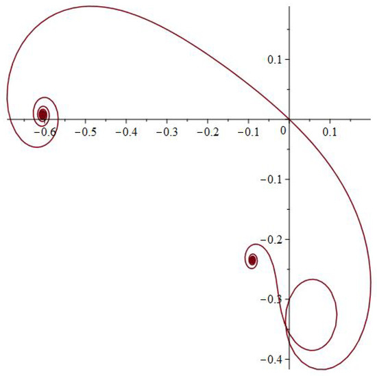
Figure 6. Picture of a curve with curvature $K(t)=10t^9+18t^2-6t+1$, for $t\in [-2,2]$.

Consider now a curve with (a slightly modified) curvature function $K(t)=10t^9+48t^2-60t+1$; its graph is very different “locally”, even if it shows a similar asymptotic behavior (see Figure 7). To avoid confusion, we point out that the “third asymptotic limit” from the middle bottom is only apparent; one can easily check it, by magnifying/restricting the graph (for example, by taking $t\in [-1.1,1.1]$).

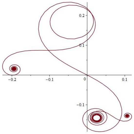
Figure 7. Picture of a curve with curvature $K(t)=10t^9+48t^2-60t+1$, for $t\in [-2,2]$.

4. Approximate Local Classification of Plane Curves

Let $c:I\to {\mathbb{R}}^2$ be a real-analytic, arc-length parameterized plane curve with (arbitrary) curvature function K. We suppose, for the sake of simplicity, that $0\in I$, $c(0)=(0,0)$ and $T(0)=(1,0)$. As previously denoted, $c(t)=({\int }_0^{t}cos\theta (s)ds,{\int }_0^{t}sin\theta (s)ds)$, where ${\theta }^{\prime }=K$ and $\theta (0)=0$.

For a fixed positive natural number n, we denote by $TA{Y}_{n}K$ the n-th polynomial from the Taylor decomposition of K around 0. For t in the convergence domain around 0, we have

$$K(t)=TA{Y}_{n}K(t)+r_n(t)·t,$$

where $r_n$ is a (unspecified but fixed) remainder function. Denote by $c_n$ the $CS$ curve associated with (the “curvature function”) $TA{Y}_{n}K$, via Formula (13). Then, $c_n(t)=({\int }_0^{t}cos{\alpha }_n(s)ds,{\int }_0^{t}sin{\alpha }_n(s)ds)$, where ${({\alpha }_n)}^{\prime }:=TA{Y}_{n}K$, with ${\alpha }_n(0)=0$.

Problem 1.

How do(es) (all/each) $c_n$(s) approximate c?

The next result offers a partial answer, involving the tangent vector fields.

Proposition 3.

With the previous notations, we have

$$\parallel T(t)-T_n(t)\parallel \le \sqrt{{\int }_0^t{(r_n(s))}^{2}ds}·\sqrt{{\displaystyle \frac{\mid t^3\mid }{3}}}$$

for t close enough to 0.

Proof. 

We replace the left norm, and we calculate

$$\parallel (cos\theta (t)-cos{\alpha }_n(t),sin\theta (t)-sin{\alpha }_n(t))\parallel =$$

$$=2\mid sin{\displaystyle \frac{\theta (t)-{\alpha }_n(t)}{2}}\mid ·\parallel (sin{\displaystyle \frac{\theta (t)+{\alpha }_n(t)}{2}},cos{\displaystyle \frac{\theta (t)+{\alpha }_n(t)}{2}})\parallel =$$

$$=2\left|sin{\displaystyle \frac{{\int }_0^t{r}_n(s)·sds}{2}}\right|\le 2\left|{\displaystyle \frac{{\int }_0^t{r}_n(s)·sds}{2}}\right|\le \sqrt{{\int }_0^t{(r_n(s))}^{2}ds}·\sqrt{\left|{\int }_0^t{s}^{2}ds\right|}.$$

We used the Cauchy–Schwarz inequality for integrals, and the fact that $\mid sinx\mid \le \mid x\mid$ for small $\mid x\mid$. □

Examples. We determine the first (few) approximations of three remarkable plane curves.

(i) When c is a line or a circle, the curvature function is already in polynomial form, so $TA{Y}_{n}K=K$ and $c_n=c$, for any positive integer n. This special property obviously occurs uniquely in this case.

(ii) Consider the spiral

$$c(t)=(({\displaystyle \frac{t}{\sqrt{2}}}+1)·sin(ln({\displaystyle \frac{t}{\sqrt{2}}}+1)),({\displaystyle \frac{t}{\sqrt{2}}}+1)·cos(ln({\displaystyle \frac{t}{\sqrt{2}}}+1))-1).$$

The curve c is arc-length parameterized, and has the curvature function

$$K(t)=-{\displaystyle \frac{1}{\sqrt{2}+t}}.$$

The first four terms from the Taylor approximation of K provide the polynomials,

$$TA{Y}_{1}K(t)=-{\displaystyle \frac{1}{\sqrt{2}}}+{\displaystyle \frac{t}{2}},TA{Y}_{2}K(t)=-{\displaystyle \frac{1}{\sqrt{2}}}+{\displaystyle \frac{t}{2}}-{\displaystyle \frac{t^2}{2\sqrt{2}}},$$

$$TA{Y}_{3}K(t)=-{\displaystyle \frac{1}{\sqrt{2}}}+{\displaystyle \frac{t}{2}}-{\displaystyle \frac{t^2}{2\sqrt{2}}}+{\displaystyle \frac{t^3}{4}},$$

$$TA{Y}_{4}K(t)=-{\displaystyle \frac{1}{\sqrt{2}}}+{\displaystyle \frac{t}{2}}-{\displaystyle \frac{t^2}{2\sqrt{2}}}+{\displaystyle \frac{t^3}{4}}-{\displaystyle \frac{t^4}{4\sqrt{2}}}.$$

Then, $c_1$, $c_2$, $c_3$, and $c_4$, given by (13), are arc-length parameterized approximations of c.

Remark 6.

An elementary well-known result tells us that any regular plane curve admits an arc-length parametrization. Unfortunately, most textbooks do not warn the reader that, in practice, there are very few chances to explicitly find one [14]. The algorithm we proposed offers a useful method of approximating a plane curve by arc-length parameterized ones, which, in addition, are “simple enough” (i.e., have polynomial curvature functions). In the sequel, we give two examples.

(i) Consider the ellipse $c(t)=(sint,2cost-2)$ and its curvature function,

$$K(t)=-{\displaystyle \frac{2}{{(co{s}^{2}t+4si{n}^{2}t)}^{\frac{3}{2}}}}.$$

The curve c has no arc-length parametrization, and one cannot find an explicit one. The first four terms from the Taylor approximation of K provide the polynomials

$$TA{Y}_{1}K(t)=-2,TA{Y}_{2}K(t)=-2+9t^2,TA{Y}_{3}K(t)=-2+9t^2,$$

$$TA{Y}_{4}K(t)=-2+9t^2-{\displaystyle \frac{147}{4}}{t}^4.$$

Then, $c_1$, $c_2$ (=$c_3$), and $c_4$, given by (13), are arc-length parameterized approximations of c.

(ii) Consider the parabola $c(t)=(t,t^2)$ and its curvature function,

$$K(t)={\displaystyle \frac{2}{{(1+4t^2)}^{\frac{3}{2}}}}.$$

The curve c is not arc-length parameterized too. The first six terms from the Taylor approximation of K provide the polynomials

$$TA{Y}_{1}K(t)=2,TA{Y}_{2}K(t)=2-12t^2,TA{Y}_{3}K(t)=2-12t^2,TA{Y}_{4}K(t)=2-12t^2+60t^4,$$

$$TA{Y}_{5}K(t)=2-12t^2+60t^4,TA{Y}_{6}K(t)=2-12t^2+60t^4-280t^6.$$

Then, $c_1$, $c_2=c_3$, $c_4=c_5$, and $c_6$, given by (13), are arc-length parameterized approximations of c.

Remark 7.

The idea to approximate the (plane) curves in order to study them by means of “simpler” objects is a very old one; the classical theory provides many geometrical notions, associated canonically to plane curves, which help their investigation: the osculating circle, the contact between two curves, osculating curves, etc.

5. Discussion

We point out some problems which might be of interest for future study.

Problem 2.

In the hypothesis of Section 4, approximate a curve c by Taylor expansions $TA{Y}_{n}c$ around 0 and compare with the previous curves $c_n$.

Problem 3.

Approximate c by Taylor expansions $TA{Y}_{n}c$ around 0, calculate the curvature functions of the latter, and compare them with the functions $TA{Y}_{n}K$.

Problem 4.

Approximate c by “asymmetric” Taylor expansion (i.e., different polynomial degrees on the two components of the curve!), calculate the curvature functions, and compare them with the functions $TA{Y}_{n}K$.

Problem 5.

Refine the classification of the curves $c_n$, with respect to additional criteria (such as multiplicity and/or the sign of the roots, etc.).

Problem 6.

Look for global properties, beyond Theorem 2. For example, there do not exist closed plane curves with a polynomial curvature function, except the circles.

Our constructions and results open a wide area of research, which may include (but is not limited to) the following topics:

-

Consider a family of remarkable polynomials (i.e., of binomial type, Jones polynomials, Abel polynomials, etc.), with special coefficients (rational, real algebraic numbers, real periods, etc.); study the curves which have this type of curvature function;

-

Study the invariance of the the CS-curves with respect to different transformations groups of the plane;

-

Is there any difference between polynomials of degree less than 5 and the others (at the level of curvature functions)?

-

Refine the theory taking into account the roots of the polynomials describing the curvature;

-

Import advanced results from the theory of polynomials (roots, etc.) into the theory of curves, via our classification;

-

Extend the previous study, by replacing the Taylor expansion by the Laurent expansion (and beyond);

-

Extend the previous study and ideas from plane curves to curves in ${\mathbb{R}}^n$, $n\ge 3$;

-

Make a separate study with properties of the new CS special functions;

-

Establish a connection between our classification and the interesting classification of plane curves from [25,26], made by using some values of the Zeta-function.

6. Conclusions

In this paper, we take several steps toward a new approach to plane curves, through the following topics:

(i) A study of the plane curves with polynomial curvature function (their general form, a classification and their asymptotic behavior);

(ii) A control algorithm for any regular plane curve, using the curvature function;

(iii) An approximate classification for regular plane curves and an algorithm for construction of approximate arc-length parametrizations;

(iv) The definition of the CS special functions, used here as a tool, but which seem to be of interest in their own;

(v) A program for development of the theory of curves, centered on the correspondence made here with the theory of polynomials.

References

- do Carmo, M.P. Differential Geometry of Curves and Surfaces; Prentice-Hall: New Jersey, NJ, USA, 1976. [Google Scholar]
- Gray, A.; Abbena, E.; Salamon, S. Modern Differential Geometry of Curves and Surfaces with Mathematica; CRC Press: Boca Raton, FL, USA, 1997. [Google Scholar]
- Montiel, S.; Ros, A. Curves and Surfaces, 2nd ed.; American Mathematical Society: Providence, RI, USA, 2009. [Google Scholar]
- O’Neill, B. Elementary Differential Geometry, 2nd ed.; Academic Press: San Diego, CA, USA, 2006. [Google Scholar]
- Zwikker, C. The Advanced Geometry of Plane Curves and Their Applications; Dover Publications, Inc.: New York, NY, USA, 1963. [Google Scholar]
- Castro, I.; Castro-Infantes, I. Plane curves with curvature depending on distance to a line. Diff. Geom. Appl. 2016, 44, 77–97. [Google Scholar] [CrossRef]
- Gielis, J.; Caratelli, D.; Shi, P.; Ricci, P.E. A Note on Spirals and Curvature. Growth Form 2020, 1, 1–8. [Google Scholar] [CrossRef][Green Version]
- Kelly, A.; Nagy, B. Reactive Nonholonomic Trajectory Generation via Parametric Optimal Control. Int. J. Robot. Res. 2003, 22, 583–601. [Google Scholar] [CrossRef]
- Koc, W. Analytical Method of Modelling the Geometric System of Communication Route. Math. Probl. Eng. 2014, 13, 679817. [Google Scholar] [CrossRef]
- Nagy, B.; Kelly, A. Trajectory generation for car-like robots using cubic curvature polynomials. In Proceedings of the 3rd International Conference on Field and Service Robotics (FSR’01), Helsinki, Finland, 11–13 June 2001; pp. 479–490. [Google Scholar]
- Šukilovic, T. Curvature based shape detection. Comput. Geom. 2015, 48, 180–188. [Google Scholar] [CrossRef]
- Surazhsky, T.; Elber, G. Metamorphosis of planar parametric curves via curvature interpolation. Int. J. Shape Model. 2002, 8, 201–216. [Google Scholar] [CrossRef]
- Cross, B.; Cripps, R.J. Efficient robust approximation of the generalized Cornu spiral. J. Comput. Appl. Math. 2015, 273, 1–12. [Google Scholar] [CrossRef]
- Gil, J. On the arc length parametrization problem. Int. J. Pure Appl. Math. 2006, 31, 401–419. [Google Scholar]
- Rababah, A. Taylor theorem for planar curves. Proc. Am. Math. Soc. 1993, 119, 803–810. [Google Scholar] [CrossRef]
- Crasmareanu, M. The flow-curvature of plane parametrized curves. Commun. Fac. Sci. Univ. Ank. 2023, 72, 417–728. [Google Scholar] [CrossRef]
- Levien, R. The Euler Spiral: A Mathematical History. Technical Report No. UCB/EECS-2008-111. Available online: http://www.eecs.berkeley.edu/Pubs/TechRpts/2008/EECS-2008-111.html (accessed on 25 November 2024).
- Wassenaar, N.P.M.; Gurney-Champion, O.J.; van Schelt, A.-S.; Bruijnen, T.; van Laarhoven, H.W.M.; Stoker, J.; Nederveen, A.J.; Runge, J.H.; Schrauben, E.M. Optimizing pseudo-spiral sampling for abdominal DCE MRI using a digital anthropomorphic phantom. Magn. Reson. Med. 2024, 92, 2051–2064. [Google Scholar] [CrossRef] [PubMed]
- Ali, J.M.; Tookey, R.M.; Ball, J.V.; Ball, A.A. The generalized Cornu spiral and its application to span generation. J. Comput. Appl. Math. 1999, 102, 37–47. [Google Scholar] [CrossRef]
- Celik, S.S.; Yayli, Y.; Guler, E. On generalized Euler spirals on E3. Int. J. Geom. 2016, 5, 5–14. [Google Scholar]
- Dillen, F. The Classification of Hypersurfaces of a Euclidean Space with Parallel Higher Order Fundamental Form. Math. Z. 1990, 203, 635–643. [Google Scholar] [CrossRef]
- Rosu, H.C.; Mancas, S.C.; Hsieh, C.C. Generalized Cornu-type Spirals and their Darboux parametric deformations. Phys. Lett. 2019, A 383, 2692–2697. [Google Scholar] [CrossRef]
- Polezhaev, A. Spirals, Their Types and Peculiarities. In Spirals and Vortices; Tsuji, K., Müller, S.C., Eds.; The Frontiers Collection; Springer: Cham, Switzerland; Berlin/Heidelberg, Germany, 2019. [Google Scholar]
- Available online: https://math.stackexchange.com/questions/2858053/generalization-of-the-sum-of-angles-formula-for-any-number-of-angles?noredirect=1&lq=1 (accessed on 25 November 2024).
- Sourmelidis, A.; Steuding, J. An atlas for all plane curves. EMS Mag. 2023, 130, 14–16. [Google Scholar] [CrossRef] [PubMed]
- Sourmelidis, A.; Steuding, J. Spirals of Riemann’s Zeta-Function—Curvature, Denseness and Universality. Math. Proc. Camb. Philos. Soc. 2024, 176, 325–338. [Google Scholar] [CrossRef]
Disclaimer/Publisher’s Note: The statements, opinions and data contained in all publications are solely those of the individual author(s) and contributor(s) and not of MDPI and/or the editor(s). MDPI and/or the editor(s) disclaim responsibility for any injury to people or property resulting from any ideas, methods, instructions or products referred to in the content. |
© 2025 by the authors. Licensee MDPI, Basel, Switzerland. This article is an open access article distributed under the terms and conditions of the Creative Commons Attribution (CC BY) license (https://creativecommons.org/licenses/by/4.0/).