Article

Sharp Coefficient Bounds for a Class of Analytic Functions Related to Exponential Function

by
Adel Salim Tayyah
1,†,
Sibel Yalçın
2,*,† and
Hasan Bayram
2,†
1
Department of Cybersecurity, College of Computer Science and Information Technology, University of Al-Qadisiyah, Diwaniyah 58002, Iraq
2
Department of Mathematics, Faculty of Arts and Sciences, Bursa Uludağ University, 16059 Bursa, Türkiye
*
Author to whom correspondence should be addressed.
These authors contributed equally to this work.
Mathematics 2025, 13(23), 3878; https://doi.org/10.3390/math13233878
Submission received: 10 November 2025 / Revised: 28 November 2025 / Accepted: 2 December 2025 / Published: 3 December 2025

Abstract

In this paper, we introduce a new class of analytic functions, denoted by S ( ν , φ ϑ , e ) , and provide illustrative examples to elucidate its properties. This class generalizes the starlike and convex functions previously defined by Khatter et al. in relation to the exponential function. A significant contribution of this work is the derivation of sharp bounds for various coefficient-related problems within this class. The computational challenges involved in deriving these bounds were effectively addressed using MathematicaTM codes. Additionally, figures illustrating the geometric properties and essential computations have been incorporated into the paper.

1. Introduction

Let A be the set of all normalized analytic functions f, represented by the Maclaurin series
f ( ζ ) = ζ + n = 2 a n ζ n , ζ D ,
where D = { ζ C : | ζ | < 1 } is the open unit disk in the complex plane C . A notable subset of A , denoted by S , consists of functions that are univalent within D . The subset S * A , defined as
S * : = f A : ζ f ( ζ ) f ( ζ ) > 0 , ζ D ,
is recognized as the class of starlike functions within D . It is well established that S * S . Similarly, the class of convex functions, denoted by C , is defined as
C : = f A : 1 + ζ f ( ζ ) f ( ζ ) > 0 , ζ D .
It is known that C S * .
Let B represent the set of analytic functions ω : D D that satisfy ω ( 0 ) = 0 . These functions are known as Schwarz functions. Given two analytic functions f and F in D , the function f is said to be subordinated to F, denoted by f ( ζ ) F ( ζ ) , if there exists a Schwarz function ω B such that f ( ζ ) = F ( ω ( ζ ) ) , ζ D . This condition implies that f ( 0 ) = F ( 0 ) and f ( D ) F ( D ) . Moreover, if F is univalent in D , then f ( ζ ) F ( ζ ) if and only if f ( 0 ) = F ( 0 ) and f ( D ) F ( D ) .
Analytic functions are often categorized into distinct families based on the geometric characteristics of their images in D . This classification provides critical insights into their structural and functional properties. Ma and Minda [1], in their 1992 work, proposed an extended subclass of the starlike family S * , denoted by S * ( φ ) . This class consists of functions f A satisfying the subordination condition
ζ f ( ζ ) f ( ζ ) φ ( ζ ) , ζ D .
The function φ is required to be analytic in D , satisfy φ ( 0 ) = 1 , have a positive real part within D , and map D onto a starlike domain with respect to 1. By modifying the function φ , a variety of subclasses related to S * can be derived. Table 1 below presents selected noteworthy research contributions that merit attention and may serve as valuable references for the interested reader.
To comprehend the rationale behind the current study, it is essential to revisit some foundational developments. One of the pivotal milestones in the history of univalent function theory was the conjecture proposed by Bieberbach in 1916, which remained unproven until De Branges established its validity in 1985 [11]. Before this major breakthrough, a great deal of mathematical effort had been devoted to tackling this conjecture. In the process, researchers succeeded in deriving coefficient bounds for several distinguished subclasses of the univalent function class  S . These efforts also led to the formulation of numerous inequalities, among them the well-known Fekete–Szegö inequality of the form | a 3 λ a 2 2 | . Closely related to this inequality is another important coefficient functional, the Hankel determinant. Pommerenke [12] provides the general definition of the Hankel determinant H p , n ( f ) for a function f A as
H p , n ( f ) : = a n a n + 1 a n + p 1 a n + 1 a n + 2 a n + p a n + p 1 a n + p a n + 2 p 2 ,
for integers p , n 1 . Specific cases of these determinants include
H 2 , 3 ( f )   =   a 3 a 5 a 4 2 , H 2 , 2 ( f )   =   a 2 a 4 a 3 2 , H 2 , 1 ( f )   =   a 3 a 2 2 , H 3 , 1 ( f )   =   2 a 2 a 3 a 4 a 4 2 a 3 3 a 2 2 a 5 + a 3 a 5 .
In particular, the quantity | H 2 , 1 ( f ) | is equivalent to the classical Fekete–Szegö functional when λ = 1 . Numerous investigations have explored the extremal value of H 2 , 1 ( f ) and established upper bounds for | H 2 , 2 ( f ) | within various subclasses of A (see [13,14,15]). Research into H 2 , 3 ( f ) has gained traction in recent years, as seen in [16,17,18]. Although the study of H 2 , 3 ( f ) remains limited, Babalola [19] was among the first to obtain non-sharp estimates for H 3 , 1 ( f ) across subclasses of S . Later, Zaprawa [20] refined these results using a novel analytical technique. More recently, sharp bounds for | H 3 , 1 ( f ) | within S * have been established by Kowalczyk et al. [21], while corresponding estimates for the class C and for functions with bounded turning were reported in [22,23], respectively. For further precise bounds of H 3 , 1 ( f ) within certain subclasses of S * , one may consult [17,24,25,26,27,28].
Khatter et al. [3] introduced a new subclass of starlike functions by selecting the function φ ϑ , e presented in the second row of Table 1,
φ ϑ , e ( ζ ) = ϑ + ( 1 ϑ ) e ζ , ϑ [ 0 , 1 ) , ζ D ,
which maps D onto the following region:
ω C : log ω ϑ 1 ϑ < 1 .
The boundary of this region, mapped by φ ϑ , e , is illustrated in Figure 1 below for three different parameter values. The authors established several notable results for this subclass. In what follows, we highlight one of these results, as it will assist in providing illustrative examples that demonstrate our main concepts, which represent a significant generalization of this subclass.
Lemma 1 
(See [3]). Let ϑ + ( 1 ϑ ) e 1 < a < ϑ + ( 1 ϑ ) e , and define ρ a by
ρ a = ( a ϑ ) ( 1 ϑ ) e 1 , if ϑ + ( 1 ϑ ) e 1 < a ϑ + 1 ϑ 2 ( e + e 1 ) , e ( 1 ϑ ) ( a ϑ ) , if ϑ + 1 ϑ 2 ( e + e 1 ) a < ϑ + ( 1 ϑ ) e .
Then,
ω C : | ω a | < ρ a ω C : log ω ϑ 1 ϑ < 1 .
Now, we define the following main class of analytic functions:
ζ f ( ζ ) + ν ζ 2 f ( ζ ) ( 1 ν ) f ( ζ ) + ν ζ f ( ζ ) φ ϑ , e ( ζ ) , ( ζ D ) ,
where 0 < ν 1 , 0 ϑ < 1 , which is denoted by S ( ν , φ ϑ , e ) .
The motivation for introducing the class S ( v , φ ϑ , e ) lies in its ability to generalize the recently introduced exponential starlike and convex classes. This class allows for a continuous transition between starlike and convex behaviors via the parameter v, introducing a controlled angular deformation through ϑ . The parameters ν and ϑ play a central geometric role in shaping the class S ( ν , φ ϑ , e ) . In particular, the class formally approaches the starlike family as ν 0 , while its behavior aligns with convex-type classes as ν 1 . Moreover, the parameter ϑ induces a deformation of the image domain φ ϑ , e ( D ) , thereby influencing the analytic structure of the class. The attached figures illustrate how the elements of this class map into the domain generated by φ ϑ , e . This clearly shows geometric deformation and the relationship between the elements of the new class and the resulting domain. This framework supports both geometric and analytic understanding compared to previous classes and justifies the introduction of this new class.
The significance of our study lies, first and foremost, in the fact that we have provided a distinguished generalization of the class introduced in [3]. The concept we propose reduces to the classes of starlike and convex functions for specific choices of the parameter  ν . Furthermore, our work takes a specialized approach by addressing the problems of coefficient estimates and Hankel determinants that were not sufficiently explored in [3]. Most importantly, all the constraints obtained in our results are sharp. The MathematicaTM program (version 13.2) played a crucial role both as a computational tool and in enhancing the applied aspect of this research. The primary motivation behind this work was to construct a class that generalizes both the starlike and convex function classes, with the distinguishing feature that its coefficient bounds and Hankel determinants are sharp. Additionally, we were encouraged to incorporate a Carathéodory function to generate a suitable domain, aligning our work with the recent stream of studies, some of which are summarized in Table 1.
It is worth noting that the class S ( ν , φ ϑ , e ) is defined in a manner analogous to Ma–Minda-type classes. In fact, it may be regarded as a Ma–Minda-type class associated with the first-order linear differential operator
L ν ( f ) ( ζ ) = ζ f ( ζ ) + ν ζ 2 f ( ζ ) ( 1 ν ) f ( ζ ) + ν ζ f ( ζ ) .
This operator interpolates between the classical starlike ζ f ( ζ ) / f ( ζ ) and its convex analogue, which clarifies the conceptual motivation behind introducing the class.
Example 1. 
For | λ | < 1 , consider the family of analytic functions
H λ = h λ ( ζ ) = ζ 1 + λ ζ : ζ D .
After performing some simple calculations, we have
Λ λ , ν ( ζ ) : = ζ h λ ( ζ ) + ν ζ 2 h λ ( ζ ) ( 1 ν ) h λ ( ζ ) + ν ζ h λ ( ζ ) = 1 + ζ λ ( 1 + 2 ν ) ( 1 + ζ λ ) ( 1 + ζ λ ( 1 + ν ) ) .
  • If ν = ν 0 0 + , then
    Λ λ , ν 0 ( ζ ) = 1 1 + ζ λ .
    Lemma 1 gives
    Λ λ , ν 0 ( ζ ) 1 = ζ λ 1 + ζ λ e ( 1 ϑ ) ( 1 ϑ ) ( ζ D ) ,
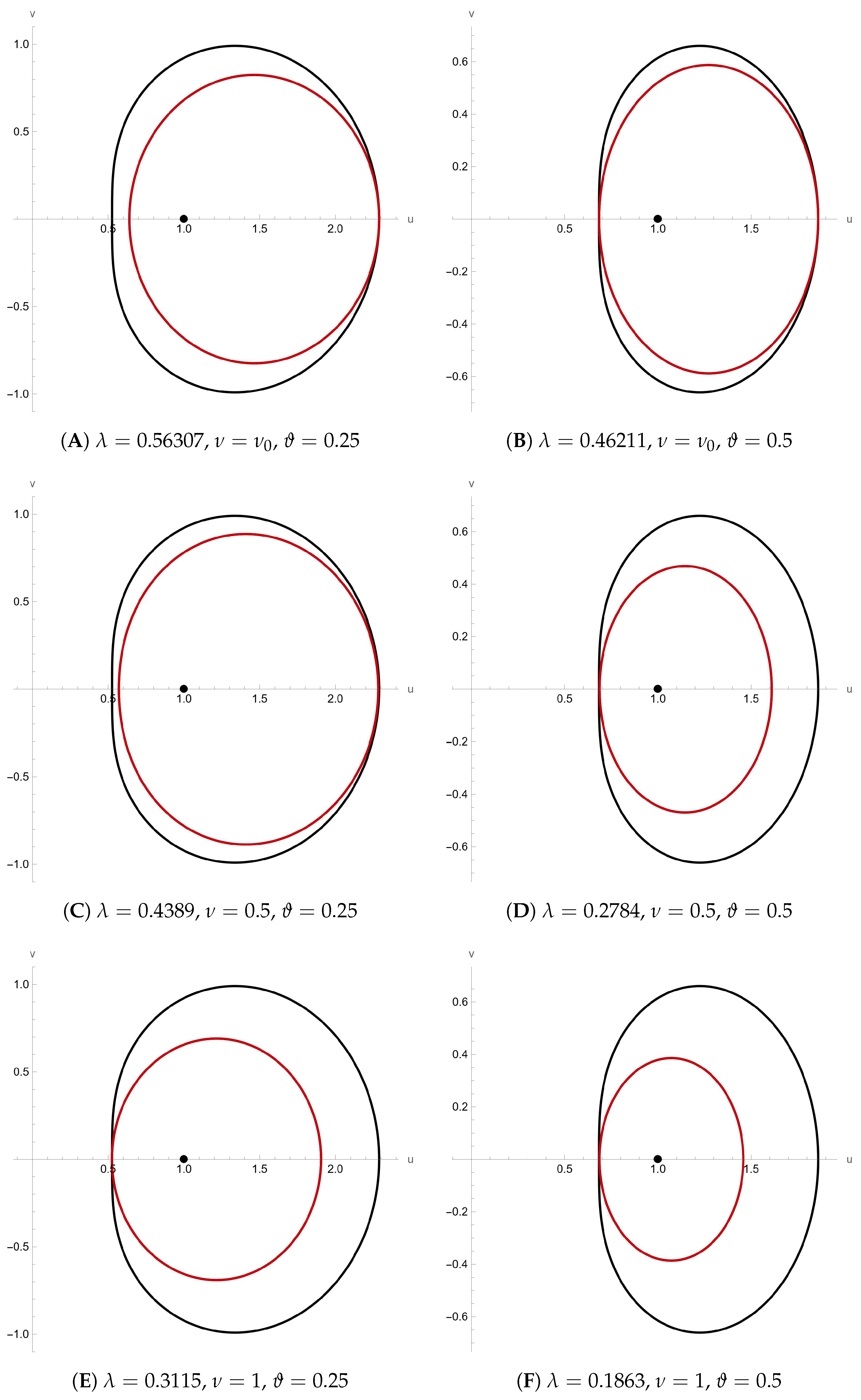
    so using the MathematicaTM program code, we obtain (see Figure 2A)
    H λ S ( ν 0 , φ 0.25 , e ) if and only if | λ | 0.56307 .
    Also (see Figure 2B),
    H λ S ( ν 0 , φ 0.5 , e ) if and only if | λ | 0.46211 .
  • If ν = 0.5 , then
    Λ λ , 0.5 ( ζ ) = 2 ( 1 + ζ λ ) ( 2 + ζ λ ) .
    Lemma 1 gives
    Λ λ , 0.5 ( ζ ) 1 = 2 ( 1 + ζ λ ) ( 2 + ζ λ ) 1 e ( 1 ϑ ) ( 1 ϑ ) ( ζ D ) ,
    so using the MathematicaTM program code, we obtain (see Figure 2C)
    H λ S ( 0.5 , φ 0.25 , e ) if and only if | λ | 0.4389 .
    Also (see Figure 2D),
    H λ S ( 0.5 , φ 0.5 , e ) if and only if | λ | 0.2784 .
  • If ν = 1 , then
    Λ λ , 1 ( ζ ) = 1 ζ λ 1 + ζ λ .
    Lemma 1 gives
    Λ λ , 1 ( ζ ) 1 = 1 ζ λ 1 + ζ λ 1 e ( 1 ϑ ) ( 1 ϑ ) ( ζ D ) ,
    so using the MathematicaTM program code, we obtain (see Figure 2E)
    H λ S ( 1 , φ 0.25 , e ) if and only if | λ | 0.3115 .
    Also (see Figure 2F),
    H λ S ( 1 , φ 0.5 , e ) if and only if | λ | 0.1863 .

2. Main Results

We now present the formula that characterizes the representation as follows:
Theorem 1. 
A function f belongs to the class S ( ν , φ ϑ , e ) if and only if it admits the following integral representation:
f ( ζ ) = ζ 1 ν ν 0 ζ 1 ν ω 1 ν ν exp 0 ω q ( x ) 1 x d x d ω , ( ζ D / { 0 } ) ,
where q ( ζ ) is an analytic function subordinate to φ ϑ , e .
Proof. 
Let ξ ( ζ ) : = ( 1 ν ) f ( ζ ) + ν ζ f ( ζ ) . Then
ζ ξ ( ζ ) ξ ( ζ ) = ζ f ( ζ ) + ν ζ 2 f ( ζ ) ( 1 ν ) f ( ζ ) + ν ζ f ( ζ ) .
Define q ( x ) : = x ξ ( x ) ξ ( x ) and k ( x ) : = ξ ( x ) x . Then q ( x ) φ ϑ , e and k ( x ) 0 . By logarithmic differentiation of k ( x ) , we obtain
k ( x ) k ( x ) = q ( x ) 1 x , ( x D ) .
Integrating (6) and simplifying, we get
ξ ( ζ ) = ζ exp 0 ζ q ( x ) 1 x d x ,
that is,
ν ζ f ( ζ ) + ( 1 ν ) f ( ζ ) = ζ exp 0 ζ q ( x ) 1 x d x .
Hence,
f ( ζ ) + 1 ν ν ζ f ( ζ ) = 1 ν exp 0 ζ q ( x ) 1 x d x .
Clearly, (7) is a linear differential equation in f, whose integrating factor is ζ ( 1 ν ) / ν . Using the normalization f ( 0 ) = 0 and f ( 0 ) = 1 determines the constant of integration, so its solution is given by
f ( ζ ) = ζ 1 ν ν 0 ζ 1 ν ω 1 ν ν exp 0 ω q ( x ) 1 x d x d ω .
   □
Example 2. 
Consider the following analytic functions:
q 1 ( ζ ) = 1 + ζ sin ζ 3 , q 2 ( ζ ) = 1 + 2 ζ e ζ 9 , q 3 ( ζ ) = 1 + 1 2 ζ 1 8 ζ 3 .
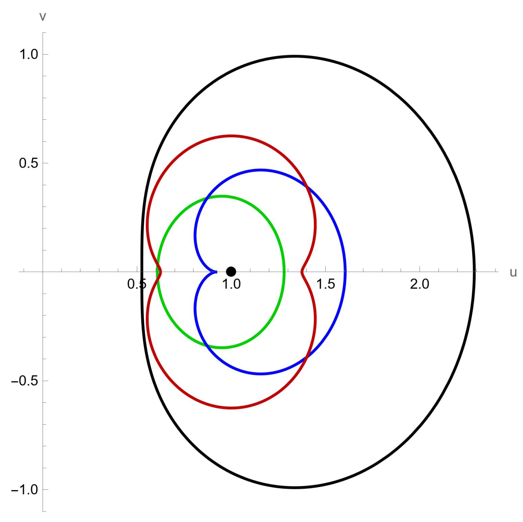
It is straightforward to verify that q i ( 0 ) = 1 and q i ( D ) φ 0.25 , e ( D ) for i = 1 , 2 , 3 . Since φ 0.25 , e S , then q i φ 0.25 , e for i = 1 , 2 , 3 (see Figure 3). Therefore, Theorem 1 implies that the functions f i ( ζ ) listed below belong to the class S ( ν , φ 0.25 , e ) :
f 1 ( ζ ) = ζ + ζ 3 6 ( 1 + 2 ν ) 7 ζ 7 6480 ( 1 + 6 ν ) + ζ 9 217728 ( 1 + 8 ν ) + , f 2 ( ζ ) = ζ + 2 ζ 2 9 ( 1 + ν ) + 11 ζ 3 81 ( 1 + 2 ν ) + 139 ζ 4 2187 ( 1 + 3 ν ) + 2087 ζ 5 78732 ( 1 + 4 ν ) + , f 3 ( ζ ) = ζ + ζ 2 2 ( 1 + ν ) + ζ 3 8 ( 1 + 2 ν ) ζ 4 48 ( 1 + 3 ν ) 7 ζ 5 384 ( 1 + 4 ν ) 19 ζ 6 3840 ( 1 + 5 ν ) + .
Example 3. 
By Theorem 1, the following formula defines infinitely many analytic functions belonging to S ( ν , φ ϑ , e ) :
K n ( ζ ) = ζ 1 ν ν 0 ζ 1 ν ω 1 ν ν exp 0 ω φ ϑ , e ( x n ) 1 x d x d ω , n = 1 , 2 , 3 ,
In particular cases, we obtain
K 1 ( ζ ) = ζ + ( ϑ 1 ) ζ 2 1 + ν + ( 3 5 ϑ + 2 ϑ 2 ) ζ 3 4 ( 1 + 2 ν ) ( 17 + 38 ϑ 27 ϑ 2 + 6 ϑ 3 ) ζ 4 36 ( 1 + 3 ν ) + ,
K 2 ( ζ ) = ζ + ( ϑ 1 ) ζ 3 2 ( 1 + 2 ν ) + ( 2 + ϑ ) ( 1 + ϑ ) ζ 5 8 ( 1 + 4 ν ) ( 1 + ϑ ) ( 16 15 ϑ + 3 ϑ 2 ) ζ 7 144 ( 1 + 6 ν ) + ,
K 3 ( ζ ) = ζ + ( ϑ 1 ) ζ 4 3 ( 1 + 3 ν ) + ( 5 7 ϑ + 2 ϑ 2 ) ζ 7 36 ( 1 + 6 ν ) ( 17 + 30 ϑ 15 ϑ 2 + 2 ϑ 3 ) ζ 10 324 ( 1 + 9 ν ) + ,
K 4 ( ζ ) = ζ + ( ϑ 1 ) ζ 5 4 ( 1 + 4 ν ) + ( 3 4 ϑ + ϑ 2 ) ζ 9 32 ( 1 + 8 ν ) ( 37 + 61 ϑ 27 ϑ 2 + 3 ϑ 3 ) ζ 13 1152 ( 1 + 12 ν ) + .
Denote by P the class of analytic functions p with ( p ( ζ ) ) > 0 for ζ D , which are given by the series expansion
p ( ζ ) = 1 + n = 1 κ n ζ n , ζ D .
Lemma 2 
(See [2,29]). Let p P , then
| κ n |     2 , n 1 ,
| κ r + n χ κ r κ n |   <   2 , 0 < χ 1 ,
| κ 2 ϱ κ 1 2 |   <   2 max 1 , | 2 ϱ 1 | , ϱ C .
Lemma 3 
(See [30]). Let 0 M 1 with M ( 2 M 1 ) N M , and let p P of the form (13). Then
| N κ 1 3 2 M κ 1 κ 2 + κ 3 |     2 .
Lemma 4 
(See [31,32]). Let p P of the form (13). Then
2 κ 2 = κ 1 2 + γ ( 4 κ 1 2 ) ,
4 κ 3 = κ 1 3 + 2 κ 1 ( 4 κ 1 2 ) γ κ 1 ( 4 κ 1 2 ) γ 2 + 2 ( 4 κ 1 2 ) ( 1 | γ | 2 ) η ,
for some γ , η C with max { | γ | , | η | } 1 .
Theorem 2. 
For 0.5 < ϑ < 1 , let f S ( ν , φ ϑ , e ) . Then,
| a n |     1 ϑ ( n 1 ) ( 1 + ( n 1 ) ν ) , for n = 2 , 3 , 4 .
These bounds are sharp by the functions K 1 , K 2 , and K 3 in (9)–(11).
Proof. 
Let f S ( ν , φ ϑ , e ) ; then there exists a Schwarz function u : D D with u ( 0 ) = 0 such that
ζ f ( ζ ) + ν ζ 2 f ( ζ ) ( 1 ν ) f ( ζ ) + ν ζ f ( ζ ) = ϑ + ( 1 ϑ ) e u ( ζ ) , ζ D .
Consider the function p P given by
p ( ζ ) = 1 + u ( ζ ) 1 u ( ζ ) = 1 + κ 1 ζ + κ 2 ζ 2 + κ 3 ζ 3 + , ζ D .
Consequently, we have
ϑ + ( 1 ϑ ) e u ( ζ ) = 1 1 2 ( 1 + ϑ ) κ 1 ζ + 1 8 ( 1 + ϑ ) ( κ 1 2 4 κ 2 ) ζ 2 + 1 48 ( 1 ϑ ) ( κ 1 3 12 κ 1 κ 2 + 24 κ 3 ) ζ 3 + 1 384 ( 1 ϑ ) ( κ 1 4 + 24 κ 1 2 κ 2 48 κ 2 2 96 κ 1 κ 3 + 192 κ 4 ) ζ 4 + ,
and
ζ f ( ζ ) + ν ζ 2 f ( ζ ) ( 1 ν ) f ( ζ ) + ν ζ f ( ζ )   =   1 + ( 1 + ν ) a 2 ζ + a 2 2 2 ν a 2 2 ν 2 a 2 2 + 2 a 3 + 4 ν a 3 ζ 2   +   ( a 2 3 3 ν a 2 3 3 ν 2 a 2 3 ν 3 a 2 3 + 2 a 2 a 3 + 6 ν a 2 a 3 + 4 ν 2 a 2 a 3   +   2 ( a 2 + ν a 2 ) ( a 2 2 + 2 ν a 2 2 + ν 2 a 2 2 a 3 2 ν a 3 )     ( a 2 + ν a 2 ) ( 3 a 3 + 6 ν a 3 ) + 3 a 4 + 9 ν a 4 ) ζ 3 .
A comparison of the initial four coefficients in (22) and (23) yields
a 2 = ( 1 + ϑ ) κ 1 2 ( 1 + ν ) ,
a 3 = ( 1 3 ϑ + 2 ϑ 2 ) κ 1 2 + 4 ( 1 ϑ ) κ 2 16 ( 1 + 2 ν ) ,
a 4 = ( 1 + ϑ ) ( 1 3 ϑ + 6 ϑ 2 ) κ 1 3 + 12 ( 1 3 ϑ ) κ 1 κ 2 + 48 κ 3 288 ( 1 + 3 ν ) .
From (14) and (24), we have
| a 2 |     1 ϑ 1 + ν .
Using (15) for 0 < χ = 1 + 3 ϑ 2 ϑ 2 4 ( 1 ϑ ) 1 (since 0.5 < ϑ < 1 ), (25) gives
| a 3 |   =   1 ϑ 4 ( 1 + 2 ν ) κ 2 1 + 3 ϑ 2 ϑ 2 4 ( 1 ϑ ) κ 1 2 1 ϑ 2 ( 1 + 2 ν ) .
Since 0.5 < ϑ < 1 , put
M = 1 3 ϑ 8 , N = 1 3 ϑ + 6 ϑ 2 48 .
Then we have
M ( 2 M 1 ) < 0.125 0.0208 < N < 0.0417 0.062 < M .
By applying (17) to (26), we obtain
| a 4 | = 1 ϑ 3 ( 1 + 3 ν ) ( 1 3 ϑ + 6 ϑ 2 ) κ 1 3 + 12 ( 1 3 ϑ ) κ 1 κ 2 + 48 κ 3 96 = 1 ϑ 3 ( 1 + 3 ν ) · 1 2 1 3 ϑ + 6 ϑ 2 48 κ 1 3 + 2 ( 1 3 ϑ ) 8 κ 1 κ 2 + κ 3 1 ϑ 3 ( 1 + 3 ν ) .
Since the sharpness is attained in Equations (9)–(11), the proof is complete and the result stands verified.    □
Theorem 3. 
Let f S ( ν , ϕ ϑ , e ) . Then for ϱ C , we have
| a 3 ϱ a 2 2 |     1 ϑ 2 ( 1 + 2 ν ) max 1 , ϑ 3 2 2 ϱ ( 1 + ϑ ) ( 1 + 2 ν ) ( 1 + ν ) 2 .
Sharpness is attained by the function K 2 in (10).
Proof. 
In light of (24), (25), and the application of (16), the desired result follows directly.    □
Corollary 1. 
Let f S ( ν , φ ϑ , e ) . Then
| a 3 a 2 2 |     1 ϑ 2 ( 1 + 2 ν ) .
Sharpness is attained by the function K 2 in (10).
Proof. 
This follows from Theorem 3, since the inequality
ϑ 3 2 2 ( 1 + ϑ ) ( 1 + 2 ν ) ( 1 + ν ) 2 < 1
holds true, as verified by the following Mathematica code:
expr = Abs [theta − 3/2 − (2∗(−1 + theta)∗(1 + 2∗nu))/(1 + nu)^2 ];
Reduce [expr < 1 && 0 < nu <= 1 && 0 < theta < 1, {nu, theta}, Reals];
test
0 < nu ≤ 1 && 0 ≤ theta < 1
The above code is used solely to verify the analytic inequalities on the compact rectangular region ( ν , ϑ ) ( 0 , 1 ] × [ 0 , 1 ) .    □
Theorem 4. 
For 0.5 < ϑ < 1 , let f S ( ν , φ ϑ , e ) . Then
| a 2 a 3 a 4 |     ϑ 1 3 ( 1 + 3 ν ) .
Sharpness is attained by the function K 3 in (11).
Proof. 
It follows from (24), (25), and (26) that
| a 2 a 3 a 4 |   =   1 ϑ 6 ( 1 + 3 ν ) N κ 1 3 2 M κ 1 κ 2 + κ 3 ,
where
N = 5 15 ν ν 2 3 ϑ ( 4 12 ν + ν 2 ) + 6 ϑ 2 ( 1 3 ν + ν 2 ) 96 ( 1 + ν ) ( 1 + 2 ν ) , M = 1 + 3 ν + ( 1 + 3 ϑ ) ν 2 16 ( 1 + ν ) ( 1 + 2 ν ) .
Therefore, we have N M , by using the following test code:
N − M = ((11 + 33∗nu − 5∗nu^2 + 18∗theta∗nu^2 + 3∗theta∗(−4 − 12∗nu + nu^2) − 6∗theta^2∗(−1 − 3∗nu + nu^2)) / (96∗(1 + nu)∗(1 + 2∗nu)));
Reduce [N − M <= 0 && 0 < nu <= 1 && 0 <= theta < 1, {nu, theta}, Reals];
test
0 < nu ≤ 1 && 0 ≤ theta < 1
Also, we verify that M ( 2 M 1 ) N for 0.5 < ϑ < 1 , by using
M = (1 + 3∗nu + (−1 + 3∗theta)∗nu^2) / (16∗(1 + nu)∗(1 + 2∗nu));
N = (−5 − 15∗nu − nu^2 − 3∗theta∗(−4 − 12∗nu + nu^2) + 6∗theta^2∗(−1 − 3∗nu + nu^2)) / (96∗(1 + nu)∗(1 + 2∗nu));
C = M∗(2∗M − 1) − N;
Reduce [C <= 0 && 0 < nu <= 1 && 0.5 <= theta < 1, {nu, theta}, Reals];
test
0 < nu ≤ 1 && 0.5 ≤ theta < 1
The codes given above accurately illustrate the inequalities being verified, and the verification was performed on the compact rectangular domain ( ν , ϑ ) ( 0 , 1 ] × ( 1 / 2 , 1 ) . These computational steps are used solely as an auxiliary tool to confirm the sign of continuous functions and do not affect the rigor of the proofs. This approach allows precise determination of the parameter ranges while preserving the completeness and validity of the proofs. Therefore, Lemma 3 leads to
| a 2 a 3 a 4 |     ϑ 1 3 ( 1 + 3 ν ) .
Thus, the result holds firmly within the logical framework of the expression, conclusively closing the proof without any ambiguity. □
Theorem 5. 
Let f S ( ν , φ ϑ , e ) . Then
| a 2 a 4 a 3 2 |     ( ϑ 1 ) 2 4 ( 1 + 2 ν ) 2 .
Sharpness is attained by the function K 2 in (10).
Proof. 
It follows from (24), (25), and (26) that
| a 2 a 4 a 3 2 | = ( ϑ 1 ) 2 4 ( 1 + 2 ν ) 2 | 13 + 52 ν + 43 ν 2 + 12 ϑ 2 ( 1 + 4 ν + ν 2 ) 12 ϑ ( 2 + 8 ν + 5 ν 2 ) 576 ( 1 + ν ) ( 1 + 3 ν ) κ 1 4 + 1 + 4 ν + ( 1 + 6 ϑ ) ν 2 24 ( 1 + ν ) ( 1 + 3 ν ) κ 1 2 κ 2 ( 1 + 2 ν ) 2 3 ( 1 + ν ) ( 1 + 3 ν ) κ 1 κ 3 + 1 4 κ 2 2 | = ( ϑ 1 ) 2 4 ( 1 + 2 ν ) 2 | 13 + 52 ν + 43 ν 2 + 12 ϑ 2 ( 1 + 4 ν + ν 2 ) 12 ϑ ( 2 + 8 ν + 5 ν 2 ) 576 ( 1 + ν ) ( 1 + 3 ν ) κ 1 4 + 1 + 4 ν + ( 1 + 6 ϑ ) ν 2 48 ( 1 + ν ) ( 1 + 3 ν ) κ 1 4 + γ κ 1 2 ( 4 κ 1 2 ) ( 1 + 2 ν ) 2 12 ( 1 + ν ) ( 1 + 3 ν ) κ 1 4 + 2 γ κ 1 2 ( 4 κ 1 2 ) γ 2 κ 1 2 ( 4 κ 1 2 ) + 2 η κ 1 ( 4 κ 1 2 ) ( 1 | γ | 2 ) + 1 16 κ 1 4 + 2 γ κ 1 2 ( 4 κ 1 2 ) + γ 2 ( 4 κ 1 2 ) 2 | .
Letting κ 1 = κ and x = | γ | in the context of Lemma 4 yields
| a 2 a 4 a 3 2 | = ( ϑ 1 ) 2 4 ( 1 + 2 ν ) 2 | 13 + 52 ν 29 ν 2 + 72 ϑ ν 2 12 ϑ ( 2 + 8 ν + 5 ν 2 ) + 12 ϑ 2 ( 1 + 4 ν + ν 2 ) 576 ( 1 + ν ) ( 1 + 3 ν ) κ 4 + ( 1 + 2 ν ) 2 12 ( 1 + ν ) ( 1 + 3 ν ) κ 2 ( 4 κ 2 ) γ 2 + 1 4 ν 13 ν 2 + 6 ϑ ν 2 48 ( 1 + ν ) ( 1 + 3 ν ) γ κ 2 ( 4 κ 2 ) ( 1 + 2 ν ) 2 6 ( 1 + ν ) ( 1 + 3 ν ) κ ( 4 κ 2 ) ( 1 | γ | 2 ) η + 1 16 γ 2 ( 4 κ 2 ) 2 | .
By taking absolute values and using the triangle inequality, we obtain
| a 2 a 4 a 3 2 | ( ϑ 1 ) 2 4 ( 1 + 2 ν ) 2 [ 13 + 52 ν 29 ν 2 + 72 ϑ ν 2 12 ϑ ( 2 + 8 ν + 5 ν 2 ) + 12 ϑ 2 ( 1 + 4 ν + ν 2 ) 576 ( 1 + ν ) ( 1 + 3 ν ) κ 4 + ( 1 + 2 ν ) 2 12 ( 1 + ν ) ( 1 + 3 ν ) κ 2 ( 4 κ 2 ) x 2 + 1 + 4 ν + 13 ν 2 6 ϑ ν 2 48 ( 1 + ν ) ( 1 + 3 ν ) x κ 2 ( 4 κ 2 ) + ( 1 + 2 ν ) 2 6 ( 1 + ν ) ( 1 + 3 ν ) κ ( 4 κ 2 ) ( 1 x 2 ) + 1 16 x 2 ( 4 κ 2 ) 2 ] : = Ψ ( x , κ ) .
Maximizing Ψ ( x , κ ) is essential at this step; accordingly,
Ψ ( x , κ ) x = ( ϑ 1 ) 2 4 ( 1 + 2 ν ) 2 [ ( 1 + 2 ν ) 2 6 ( 1 + ν ) ( 1 + 3 ν ) κ 2 ( 4 κ 2 ) x + 1 + 4 ν + 13 ν 2 6 ϑ ν 2 48 ( 1 + ν ) ( 1 + 3 ν ) κ 2 ( 4 κ 2 ) ( 1 + 2 ν ) 2 3 ( 1 + ν ) ( 1 + 3 ν ) κ ( 4 κ 2 ) x + 1 8 x ( 4 κ 2 ) 2 ] .
It is evident that Ψ ( x , κ ) x 0 for all x [ 0 , 1 ] . Therefore, the function Ψ ( x , κ ) attains its maximum at x = 1 , which leads to
Ψ ( κ ) : = Ψ ( 1 , κ ) = ( ϑ 1 ) 2 4 ( 1 + 2 ν ) 2 [ 13 + 52 ν 29 ν 2 + 72 ϑ ν 2 12 ϑ ( 2 + 8 ν + 5 ν 2 ) + 12 ϑ 2 ( 1 + 4 ν + ν 2 ) 576 ( 1 + ν ) ( 1 + 3 ν ) κ 4 + ( 1 + 2 ν ) 2 12 ( 1 + ν ) ( 1 + 3 ν ) κ 2 ( 4 κ 2 ) + 1 + 4 ν + 13 ν 2 6 ϑ ν 2 48 ( 1 + ν ) ( 1 + 3 ν ) κ 2 ( 4 κ 2 ) + 1 16 ( 4 κ 2 ) 2 ] .
We now aim to identify the optimal value of κ that yields the maximum of Ψ ( κ ) . Hence,
Ψ ( κ ) = ( 1 + ϑ ) 2 24 96 ν + 264 ν 2 144 ϑ ν 2 κ 576 ( 1 + ν ) ( 1 + 2 ν ) 2 ( 1 + 3 ν ) + ( 1 + ϑ ) 2 11 24 ϑ + 12 ϑ 2 + ( 44 96 ϑ + 48 ϑ 2 ) ν 269 ν 2 + 84 ϑ ν 2 + 12 ϑ 2 ν 2 κ 3 576 ( 1 + ν ) ( 1 + 2 ν ) 2 ( 1 + 3 ν ) .
After setting it to 0, we obtain the three roots:
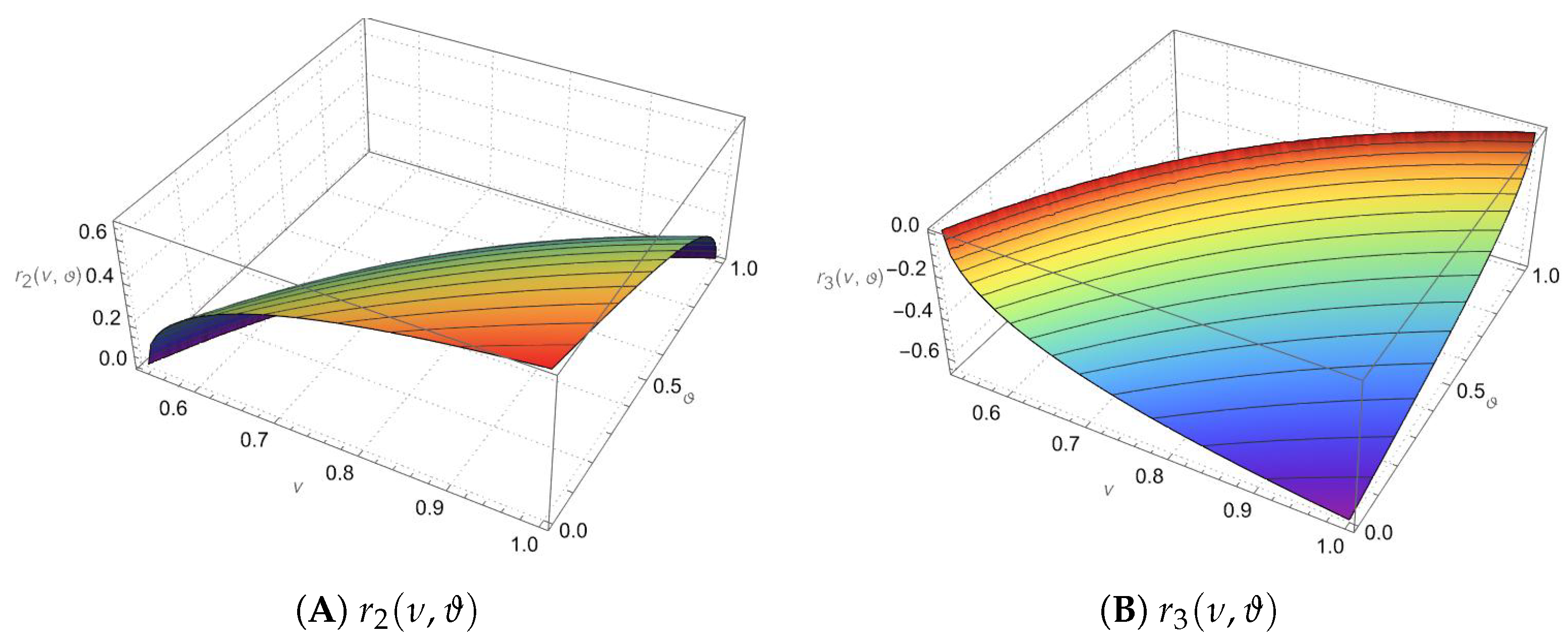
r 1 = 0 [ 0 , 2 ] , r 2 = 2 6 ( 1 ϑ ) 1 + 4 ν 11 ν 2 + 6 ϑ ν 2 11 2 ϑ + 49 ϑ 2 48 ϑ 3 + 12 ϑ 4 44 ν 8 ϑ ν + 196 ϑ 2 ν 192 ϑ 3 ν +   48 ϑ 4 ν 269 ν 2 + 622 ϑ ν 2 425 ϑ 2 ν 2 + 60 ϑ 3 ν 2 + 12 ϑ 4 ν 2 [ 0 , 2 ] , r 3 = 2 6 ( 1 + ϑ ) 1 + 4 ν 11 ν 2 + 6 ϑ ν 2 11 2 ϑ + 49 ϑ 2 48 ϑ 3 + 12 ϑ 4 44 ν 8 ϑ ν + 196 ϑ 2 ν 192 ϑ 3 ν +   48 ϑ 4 ν 269 ν 2 + 622 ϑ ν 2 425 ϑ 2 ν 2 + 60 ϑ 3 ν 2 + 12 ϑ 4 ν 2 [ 0 , 2 ] .
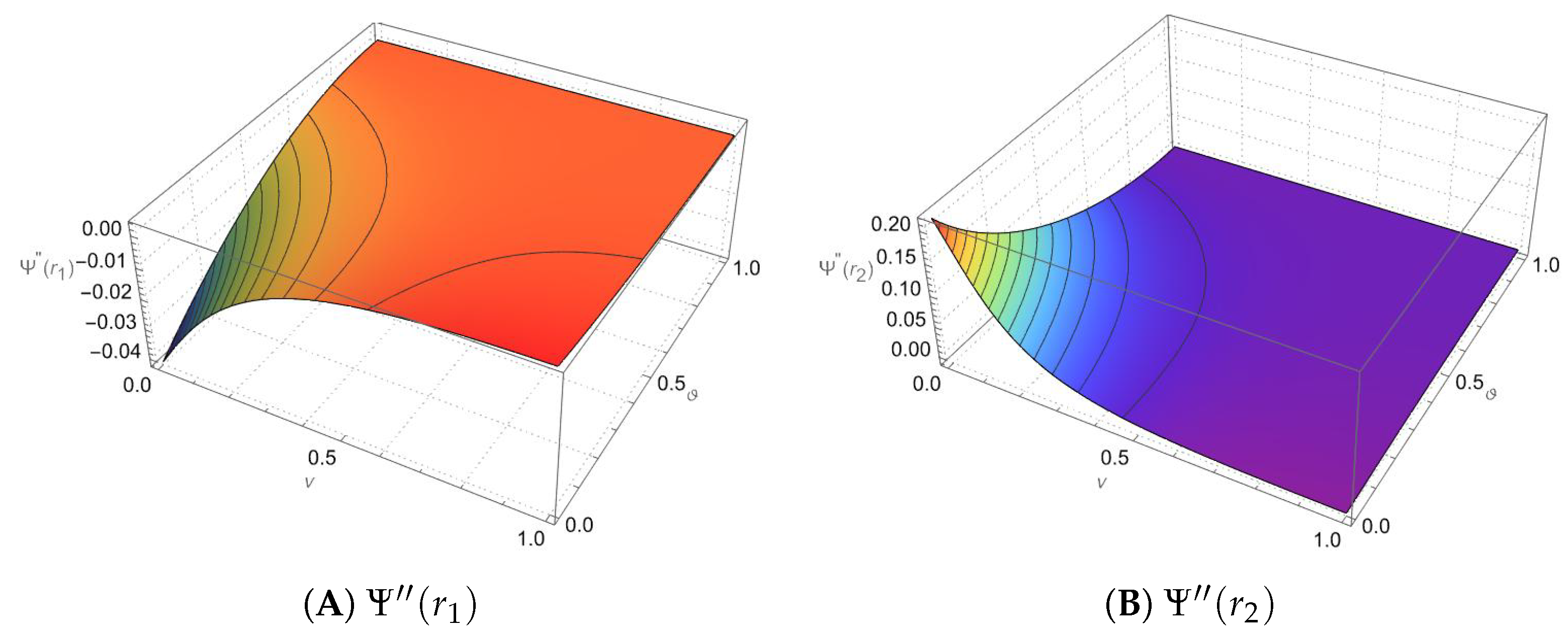
See Figure 4A,B. Since Ψ ( r 1 ) < 0 (see Figure 5A), the maximum is attained at r 1 . Similarly, since Ψ ( r 2 ) > 0 (see Figure 5B), the minimum is attained at r 2 . Therefore,
| a 2 a 4 a 3 2 |     Ψ ( 1 , 0 ) = ( ϑ 1 ) 2 4 ( 1 + 2 ν ) 2 .
Thus, the proof is established, affirming the validity of the result. □

3. Conclusions

This study provides a comprehensive investigation of the new class of analytic functions S ( ν , φ ϑ , e ) , emphasizing the challenge of deriving sharp bounds for the coefficients despite the presence of multiple influencing parameters. The most significant result obtained is the use of the solution of a linear differential equation to construct the general formula of functions belonging to this class, offering a systematic and clear method for generating precise examples and analyzing their properties. Moreover, the study allowed us to obtain exact extremal bounds for the initial coefficients and to illustrate the impact of the parameter ν in transitioning between starlike and convex behaviors. Consequently, this work provides a new framework for studying coefficient problems and subordination conditions in analytic function classes, contributing effectively to the development of geometric analysis methods.

Author Contributions

Conceptualization, A.S.T.; methodology, A.S.T. and S.Y.; validation, S.Y.; formal analysis, H.B.; investigation, A.S.T.; project administration, H.B.; writing—original draft preparation, A.S.T.; writing—review and editing, H.B.; supervision, S.Y. All authors have read and agreed to the published version of the manuscript.

Funding

This research received no external funding.

Data Availability Statement

The original contributions presented in this study are included in the article. Further inquiries can be directed to the corresponding author.

Conflicts of Interest

The authors declare that they have no conflicts of interest.

References

  1. Ma, W.C.; Minda, D. A unified treatment of some special classes of univalent functions. In Proceedings of the Conference on Complex Analysis, Tianjin, China, 19–23 June 1992; International Press: Cambridge, MA, USA, 1994; pp. 157–169. [Google Scholar]
  2. Sharma, K.; Jain, N.K.; Ravichandran, V. Starlike functions associated with a cardioid. Afr. Math. 2016, 27, 923–939. [Google Scholar] [CrossRef]
  3. Khatter, K.; Ravichandran, V.; Sivaprasad Kumar, S. Starlike functions associated with exponential function and the lemniscate of Bernoulli. Rev. R. Acad. Cienc. Exactas Fís. Nat. Ser. A Math. RACSAM 2019, 113, 233–253. [Google Scholar] [CrossRef]
  4. Raina, R.K.; Sharma, P.; Sokół, J. Certain classes of analytic functions related to the crescent-shaped regions. Izv. Nats. Akad. Nauk Armenii Math. 2018, 53, 83–93. [Google Scholar] [CrossRef]
  5. Yunus, Y.; Halim, S.A.; Akbarally, A.B. Subclass of starlike functions associated with a limacon. AIP Conf. Proc. 2018, 1974, 030023. [Google Scholar] [CrossRef]
  6. Goel, P.; Kumar, S.S. Certain class of starlike functions associated with modified sigmoid function. Bull. Malays. Math. Sci. Soc. 2019, 42, 2121–2137. [Google Scholar] [CrossRef]
  7. Cho, N.E.; Kumar, V.; Kumar, S.S.; Ravichandran, V. Radius problems for starlike functions associated with the sine function. Bull. Iran. Math. Soc. 2019, 45, 213–232. [Google Scholar] [CrossRef]
  8. Ullah, K.; Srivastava, H.M.; Rafiq, A.; Arif, M.; Arjika, S. A study of sharp coefficient bounds for a new subfamily of starlike functions. J. Inequal. Appl. 2021, 2021, 194. [Google Scholar] [CrossRef]
  9. Tayyah, A.S.; Hadi, S.H.; Wang, Z.-G.; Lupaş, A.A. Classes of Ma–Minda type analytic functions associated with a kidney-shaped domain. AIMS Math. 2025, 10, 22445–22470. [Google Scholar] [CrossRef]
  10. Tayyah, A.S.; Atshan, W.G. Starlikeness and Bi-Starlikeness Associated with a New Carathéodory Function. J. Math. Sci. 2025, 290, 232–256. [Google Scholar] [CrossRef]
  11. De Branges, L. A proof of the Bieberbach conjecture. Acta Math. 1985, 154, 137–152. [Google Scholar] [CrossRef]
  12. Pommerenke, C. On the coefficients and Hankel determinants of univalent functions. J. Lond. Math. Soc. 1966, 41, 111–122. [Google Scholar] [CrossRef]
  13. Janteng, A.; Halim, S.A.; Darus, M. Coefficient inequality for a function whose derivative has a positive real part. J. Inequal. Pure Appl. Math. 2006, 7, 50. [Google Scholar]
  14. Janteng, A.; Halim, S.A.; Darus, M. Hankel determinant for starlike and convex functions. Int. J. Math. Anal. 2007, 1, 619–625. [Google Scholar]
  15. Obradović, M.; Tuneski, N. Hankel determinants of second and third order for the class S of univalent functions. Math. Slovaca 2021, 71, 649–654. [Google Scholar] [CrossRef]
  16. Obradović, M.; Tuneski, N. Two types of the second Hankel determinant for the class U and the general class S. Acta Comment. Univ. Tartu. Math. 2023, 27, 59–67. [Google Scholar] [CrossRef]
  17. Riaz, A.; Raza, M.; Binyamin, M.A.; Saliu, A. The second and third Hankel determinants for starlike and convex functions associated with Three-Leaf function. Heliyon 2023, 9, 12748. [Google Scholar] [CrossRef] [PubMed]
  18. Zaprawa, P. On Hankel determinant H2(3) for univalent functions. Results Math. 2018, 73, 89. [Google Scholar] [CrossRef]
  19. Babalola, K.O. On H3(1) Hankel determinant for some classes of univalent functions. In Inequality Theory and Applications; Cho, Y.J., Ed.; Nova Science Publishers: New York, NY, USA, 2010; Volume 6, pp. 1–7. [Google Scholar]
  20. Zaprawa, P. Third Hankel determinants for subclasses of univalent functions. Mediterr. J. Math. 2017, 14, 19. [Google Scholar] [CrossRef]
  21. Kowalczyk, B.; Lecko, A.; Thomas, D.K. The sharp bound of the third Hankel determinant for starlike functions. Forum Math. 2022, 34, 1249–1254. [Google Scholar] [CrossRef]
  22. Kowalczyk, B.; Lecko, A. The sharp bound of the third Hankel determinant for functions of bounded turning. Bol. Soc. Math. Mex. 2021, 27, 69. [Google Scholar] [CrossRef]
  23. Kowalczyk, B.; Lecko, A.; Sim, Y.J. The sharp bound for the Hankel determinant of the third kind for convex functions. Bull. Aust. Math. Soc. 2018, 97, 435–445. [Google Scholar] [CrossRef]
  24. Banga, S.; Kumar, S.S. The sharp bounds of the second and third Hankel determinants for the class SL*. Math. Slovaca 2020, 70, 849–862. [Google Scholar] [CrossRef]
  25. Lecko, A.; Sim, Y.J.; Śmiarowska, B. The sharp bound of the Hankel determinant of the third kind for starlike functions of order 1/2. Complex Anal. Oper. Theory 2019, 13, 2231–2238. [Google Scholar] [CrossRef]
  26. Riaz, A.; Raza, M. The third Hankel determinant for starlike and convex functions associated with lune. Bull. Sci. Math. 2023, 187, 103289. [Google Scholar] [CrossRef]
  27. Tayyah, A.S.; Hadi, S.H.; Alatawi, A.; Abbas, M.; Bagdasar, O. Sharp Functional Inequalities for Starlike and Convex Functions Defined via a Single-Lobed Elliptic Domain. Mathematics 2025, 13, 3367. [Google Scholar] [CrossRef]
  28. Riaz, A.; Raza, M.; Thomas, D.K. Hankel determinants for starlike and convex functions associated with sigmoid functions. Forum Math. 2022, 34, 137–156. [Google Scholar] [CrossRef]
  29. Keogh, F.R.; Merkes, E.P. A coefficient inequality for certain classes of analytic functions. Proc. Am. Math. Soc. 1969, 20, 8–12. [Google Scholar] [CrossRef]
  30. Efraimidis, I. A generalization of Livingston’s coefficient inequalities for functions with positive real part. J. Math. Anal. Appl. 2016, 435, 369–379. [Google Scholar] [CrossRef]
  31. Ravichandran, V.; Verma, S. Bound for the fifth coefficient of certain starlike functions. C. R. Math. 2015, 353, 505–510. [Google Scholar] [CrossRef]
  32. Pommerenke, C. Univalent Functions; Vandenhoeck and Ruprecht: Göttingen, Germany, 1975. [Google Scholar]
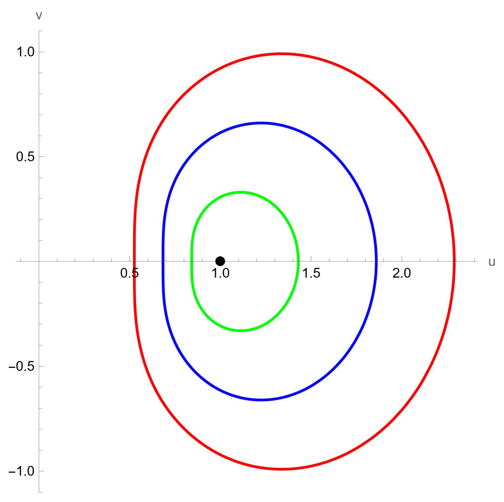
Figure 1. Plot the boundary of φ ϑ , L ( D ) at ϑ = 0.25 , ϑ = 0.5 , and ϑ = 0.75 as colors red, blue, and green, respectively.
Mathematics 13 03878 g001
Figure 2. Representation of the regions Λ ( λ , ν ) ( D ) φ ( ϑ , e ) ( D ) for various parameter values.
Mathematics 13 03878 g002
Figure 3. Plot boundaries of q 1 ( D ) , q 2 ( D ) , and q 3 ( D ) , as colors green, blue, and red, respectively.
Mathematics 13 03878 g003
Figure 4. Plot of the roots r 2 and r 3 .
Mathematics 13 03878 g004
Figure 5. Plot of the second derivatives at the roots r 1 and r 2 , specifically Ψ ( r 1 ) and Ψ ( r 2 ) .
Mathematics 13 03878 g005
Table 1. Some functions φ used in defining special cases of the Ma–Minda function class.
Function φ ( ζ ) YearReference
φ C ( ζ ) = 1 + 4 ζ 3 + 2 ζ 2 3 2016[2]
φ ϑ , e ( ζ ) = ϑ + ( 1 ϑ ) e ζ , ϑ [ 0 , 1 ) 2017[3]
φ ϑ , L ( ζ ) = ϑ + ( 1 ϑ ) 1 + ζ , ϑ [ 0 , 1 ) 2017[3]
φ ( ζ ) = ζ + 1 + ζ 2 2018[4]
φ lim ( ζ ) = 1 + 2 ζ + ζ 2 2 2018[5]
φ SG ( ζ ) = 2 1 + e ζ 2019[6]
φ S ( ζ ) = 1 + sin ζ 2019[7]
φ tanh ( ζ ) = 1 + tanh ζ 2021[8]
φ k ( ζ ) = 2 4 ( 1 + e 2 ζ ) 2 3 2025[9]
φ H ( ζ ) = 1 + ζ + 1 3 ζ 2 1 9 ζ 3 2025[10]
Disclaimer/Publisher’s Note: The statements, opinions and data contained in all publications are solely those of the individual author(s) and contributor(s) and not of MDPI and/or the editor(s). MDPI and/or the editor(s) disclaim responsibility for any injury to people or property resulting from any ideas, methods, instructions or products referred to in the content.