Surrogate Model-Based Optimization of a Dual-Shield Total Temperature Probe for Aero-Engine Applications

Abstract

The design of high-precision total temperature probes for aero-engines is constrained by the massive computational cost of high-fidelity simulations. This paper overcomes this barrier by introducing a surrogate model-based optimization framework for a dual-shield probe. A computationally efficient data-driven framework is established, merging conjugate-heat-transfer Computational Fluid Dynamics (CFDs), a Support Vector Regression (SVR) model, and a Genetic Algorithm (GA), which collectively replace the traditional costly design loop. The surrogate model’s exceptional predictive fidelity is confirmed, and this approach obtains improvement in measurement accuracy, successfully reducing the temperature deviation and meeting the stringent requirement. Finally, the demonstrated framework is geometry-agnostic, establishing a generalizable and cost-effective strategy for the rapid design of high-performance thermometric components in gas turbine systems.

1. Introduction

The total temperature probe is a crucial sensor in testing aero engines and high-temperature airflows. Its measurement accuracy directly affects the engine’s performance evaluation and safety control [1,2]. Much research has been conducted on improving measurement accuracy and calibrating probes in aircraft engines [3,4]. In practical applications, the coupling between thermodynamics and fluid mechanics under complex flow conditions leads to significant errors in total temperature measurements, primarily radiation, conduction, and velocity errors [5]. Meanwhile, due to issues with radiative heat dissipation and the limited installation space for dedicated temperature sensors, it is impossible to eliminate errors solely by designing a special head structure. Therefore, during the design stage, it is necessary to optimize the probe’s shape as much as possible to improve its accuracy and to calibrate its measurement accuracy before use [6,7]. However, the inherent errors (e.g., radiation, conduction, and velocity) of standard probes, as well as the uneven airflow distribution caused by limited installation space, can pose challenges to probe design and calibration.

A large number of experiments have been carried out to optimize and calibrate probes [8,9]. These experimental results provide an essential basis for studying the total temperature error. However, the experimental methods are time-consuming. Especially, some repetitive work and the high cost in extreme cases have led to difficulties in experimental research. Furthermore, the source causing the total temperature thermocouple error cannot be accurately calibrated through experiments [10]. Numerical simulation offers an efficient means to optimize probe performance and analyze error mechanisms [11]. It can reveal the influence patterns of flow field interference, heat conduction, and radiation through multiphysics field-coupling simulation [12,13]. Compared to theoretical methods, numerical simulations have fewer assumptions and a broader range of applications. Unlike experimental methods, they do not require standard probes to measure flow field temperature, making them more efficient and cost-effective. They can also provide more physical phenomena and values within the flow field.

In recent years, with the advancement of CFD and conjugate heat transfer methods, an increasing number of scholars have applied numerical simulation technology to conduct extensive research on total temperature probes. Villafañe et al. [14] from the Von Karman Institute of Fluid Dynamics used numerical simulation methods for conjugate heat transfer to analyze probe response and various sources of temperature errors. Matas et al. [15] employed thermal network simulation methods and numerical simulation approaches to simulate multipoint total temperature probes for compressors and also compared the effects of different Reynolds-Averaged Navier–Stokes turbulence models on numerical simulation temperature measurement deviations. Wang et al. [16] designed a new shielded total temperature probe for relatively low-temperature gas measurement; the probe’s characteristics and various error sources were analyzed using the conjugate heat transfer simulation method.

The gas flow and temperature fields in the engine are complex. To obtain a relatively accurate temperature field, probes are usually installed at different positions. Due to differences in installation locations, different flow field conditions, and temperature ranges, it is difficult for universal probes to achieve high-precision measurements in all situations. Therefore, it is usually necessary to separately design the structural parameters of probes for different working conditions and conduct calibration tests, which involves a significant amount of repetitive work. Wang et al. [7] combined numerical simulation with parametric design to streamline this process. The parametric method handles probe sizing, while numerical simulation conducts experimental analysis. This integration reduces repetitive design and calibration work, thereby enhancing the optimization of probe performance. Structural optimization represents a well-established approach for enhancing thermo-fluidic system performance, as similarly demonstrated in the optimization of porous cavity flow and heat transfer [17].

However, this method relies on high-precision CFD simulations, and each simulation takes considerable time. As the dimension of the optimization parameters increases, the computational cost rises significantly, making it challenging to meet the requirements for rapid iteration [18,19]. Meanwhile, this method relies on numerical simulation rather than experiments, making it difficult to fully utilize experimental data, such as wind tunnel calibration results, in the design and calibration of probes.

Surrogate modeling is a method for creating mathematical approximations of complex systems. Machine learning-based surrogate models can bypass computationally expensive simulations and have been widely adopted in CFD to accelerate design optimization and uncertainty quantification. They have been successfully applied across various domains, including turbulent modeling, flow control, and design optimization. Du et al. [20] proposed a deep learning-based surrogate for rapid prediction around complex 3D geometries, enabling efficient prediction of patient-specific aortic hemodynamics with a 100,000× speedup over traditional CFD simulations. Wilson et al. [21] built a surrogate model to predict wake-internal wind speeds from CFD data, achieving accurate interpolation of 3D wake velocities and extrapolation to novel wind speeds with low error, and Elkarii et al. [22] developed one for predicting pressure drop in slurry flow, proposing a new friction factor correlation based on 525 CFD data points with over 85% prediction accuracy. These methods are typically trained on data from high-fidelity numerical models, such as CFD. They can accurately predict outcomes with significantly less computational effort than the original simulations, making them an effective solution for scenarios requiring rapid analysis.

In the specific context of temperature measurement and sensor design, several studies demonstrate the potential of surrogate modeling. For instance, Jeon et al. [23] developed a Deep-Neural-Network-based surrogate model to optimize gas detector layouts, while Morozova et al. [24] created a CFD-driven surrogate model to predict flow parameters in mechanically ventilated rooms. These successful applications provide strong precedents and confidence for the present study to employ an SVR surrogate model to optimize total temperature probes.

In the design and optimization of instrumentation and precision sensors, machine learning surrogate models have demonstrated significant advantages for high-end equipment. For instance, Zhu et al. [25] applied an improved Back Propagation Neural Network (BPNN) and a genetic algorithm to optimize 11 thermal design parameters of a space telescope. Similarly, Zhang et al. [26] built a CatBoost surrogate to predict motor efficiency and torque for an aerospace system, and coupled it with the Non-dominated Sorting Genetic Algorithm-III algorithm to optimize 71 structural parameters, improving performance while reducing computational overhead. In microelectronic packaging, Shan et al. [27] used a Kriging surrogate model to rapidly evaluate how nozzle and backflow chamber structures affect jetting velocity and volume, and validated the optimized design experimentally via multi-objective genetic algorithm optimization.

To apply the surrogate model’s predictive ability to the design of structural parameters, a powerful optimization method must work in conjunction with it. For such engineering optimization problems characterized by multivariate, nonlinear, and computationally expensive objective functions, population-based global optimization algorithms, such as GA, have been proven to be an ideal choice. Zhu et al. [25] used a Genetic Algorithm to optimize the parameters of their improved BP neural network surrogate model and to find the optimal thermal design parameters for a space telescope. Zhang et al. [26] employed the Non-dominated Sorting Genetic Algorithm-III algorithm, an advanced multi-objective Genetic Algorithm, to achieve rapid multi-objective optimization of 71 structural parameters for a complex electromechanical system. Shan et al. [27] applied a bi-objective Genetic Algorithm to concurrently optimize the dispensing velocity and the dispensed volume in their surrogate model-based study of a jetting system. Li et al. [28] utilized a Multi-Objective Genetic Algorithm to optimize the heat dissipation performance of an air-cooling battery pack based on a Kriging surrogate model. Gu et al. [29] adopted the Non-dominated Sorting Genetic Algorithm-II algorithm to solve the computationally expensive multi-objective optimization problem of a high-speed permanent magnet synchronous machine, leveraging surrogate models to reduce the FEM calculation burden. These algorithms can effectively avoid local optima and operate without gradient information, enabling them to collaborate efficiently with the surrogate model to jointly address challenges in probe optimization.

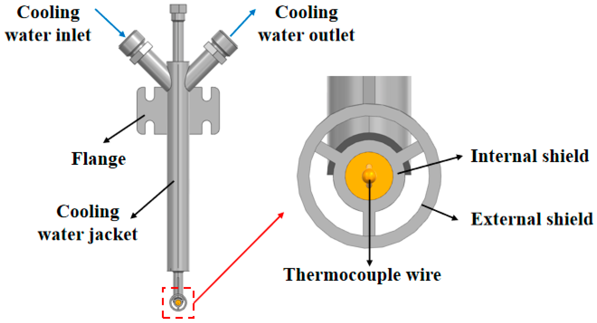
The shielded total temperature probe is typically used to measure the total temperature of high-temperature, high-speed gas flows, particularly to determine the exhaust temperature of aeroengine tail nozzles [5,30]. The key to improving the accuracy of flow field temperature measurement by probes lies in stopping the flow field. The probe’s shielding cover plays an important role [31]. Different parameters of the shielding cover have varying degrees of hindrance to radiant heat transfer. Optimizing the design of the shielding cover is crucial for enhancing the temperature measurement accuracy of probes.

Despite the critical role of total temperature probes in aero-engine monitoring, their design optimization faces significant challenges. Traditional approaches, which rely heavily on experimental calibration or high-fidelity conjugate heat transfer CFD simulations, are often prohibitively time-consuming and computationally expensive for rapid design iterations. This is particularly true when dealing with multivariate geometric parameters under extreme operating conditions. Consequently, there is an urgent need for an efficient and automated optimization framework that can achieve high measurement accuracy for complex design spaces, significantly shorten the development cycle, and reduce computational costs. Therefore, this research aims to develop a design optimization framework based on surrogate models to address the limitations of traditional methods in the design of dual-shielded total temperature probes.

This study successfully developed and validated a surrogate model-based optimization framework for the design of a dual-shield total temperature probe. The main contributions are as follows:

(1)

We have proposed an effective optimization methodology that integrates CFD, SVR surrogate model, and GA optimization. This framework effectively replaces traditional, expensive numerical simulation and experimental methods and can quickly achieve global optimization of probe structure parameters at relatively low computational cost.

(2)

The framework delivers a substantial performance improvement. Through this approach, the probe’s temperature measurement deviation was successfully reduced to within the acceptable range, demonstrating a significant improvement in accuracy. This optimized design meets the stringent accuracy requirement for critical aero-engine applications.

(3)

The developed methodology is geometry-agnostic and extensible. The core workflow is not limited to the specific probe geometry presented here. It provides a cost-effective and generalizable framework for the optimized design of various temperature sensors and similar aerothermodynamic components across a wide range of operating conditions.

In Section 2, numerical simulations are used to generate a training dataset for a surrogate model. This enables the rapid prediction of temperature measurement errors under various structural parameters. In Section 3, a genetic algorithm based on a surrogate model is applied to efficiently find the optimal probe structure. This approach significantly reduces computational costs, enhances optimization efficiency, and provides a novel method for designing high-precision total temperature probes. Finally, the conclusion is given in Section 4.

2. Numerical Simulation Analysis

2.1. Research Object

The research object of this paper is the double-shielded water-cooled standard total temperature probe, whose structure comprises internal and external shields, a thermocouple wire, a flange, a water-cooled structure, and sealing components, as shown in Figure 1. The sensing part, indicated by the orange component in Figure 1, is made of precious metals, with the sensitive element being an iridium-rhodium alloy probe of 0.5 mm diameter. The support structure operating in the high-temperature airflow is divided into two sections: the portion supporting the sensing element is dry-fired and fabricated from precious metal, while the external section exposed to the high-temperature airflow is water-cooled and constructed from superalloy.

According to the physical characteristics of the total temperature probe, the calculation domain is divided into three parts: the first part is the air fluid domain in contact with the sensing part of the probe, the second part is the cooling water domain involved in the total temperature probe cooling, and the third part is the solid domain of the total temperature probe structure. The structure diagram is shown in Figure 2, where the air fluid domain is consistent with the actual test environmental parameters of the total temperature probe.

2.2. Numerical Method

Numerical simulations were performed using the commercial software ANSYS Fluent 2022R1. A conjugate heat transfer model was employed to solve the three-dimensional, steady-state Navier–Stokes equations using the Semi-Implicit Method for Pressure Linked Equations algorithm. For spatial discretization, the Least Squares Cell-Based scheme was utilized due to its accuracy and suitability for the polyhedral mesh employed in this study.

The Shear Stress Transport (SST) turbulence model was selected for its demonstrated accuracy in predicting flows with adverse pressure gradients and separation, which are anticipated around the probe geometry. This choice is supported by its proven capability in complex convective heat transfer simulations, as evidenced in the uncertainty and sensitivity analysis of [32]. The model maintains robustness throughout the boundary layer, making it particularly suited for the present conjugate heat transfer problem.

The fluid domain (air) was treated as an ideal gas to account for compressibility effects at the high Mach number (0.6) condition. The dynamic viscosity of air was calculated using Sutherland’s formula, a standard semi-empirical relation for temperature-dependent viscosity [33]. The thermal conductivity was subsequently determined by the solver based on kinetic theory and its relation to the dynamic viscosity. Radiation heat transfer was modeled using the Discrete Ordinates model, which is capable of accounting for the participating media effects of the air within the computational domain.

Due to the complexity of the total temperature sensor model in this study, a polyhedral mesh was employed for grid generation. To ensure simulation accuracy, the mesh was refined around the total temperature probe, and boundary layers were generated on all fluid domain walls. The minimum grid size in the entire computational domain was set to one-tenth of the total temperature probe wire diameter, while the maximum grid size was set to one-fiftieth of the fluid domain diameter. Additionally, the entire computational region was refined with the total temperature probe as the center, using a growth rate of 1.05. Ultimately, the total number of grid cells was approximately 3 million, with about 200,000 in the solid domain, 300,000 in the cooling water fluid domain, and 2.5 million in the air fluid domain. The resulting mesh is shown in Figure 3.

In the calculation conditions, the incoming flow Mach number within the domain is set to 0.6. The total temperature of the incoming flow is set to 2300 K, while the environmental pressure is maintained at 1.0 MPa. The cooling water flow rate is set to 1.0 kg/s. The heat transfer coefficient is 25 W/(m²·K), and the ambient temperature is 293.15 K. The emissivity of the shield is specified as 0.85, the emissivity of the probe wire is 0.9, and the emissivity of the ball welding is also set to 0.9.

2.3. Error Analysis

The primary sources of temperature measurement error $\Delta T$ of the total temperature probe, are velocity error ${\sigma }_w$, thermal conductivity error ${\sigma }_c$ and radiation error ${\sigma }_r$, among which the velocity error ${\sigma }_w$ refers to the deviation between the total temperature $T_0$ of the air stream and the effective temperature $T_g$ of the air stream, as shown in Equation (1):

$${\sigma }_w=T_0-T_g$$

(1)

Thermal conductivity error ${\sigma }_c$ means that there is a temperature gradient between the measuring end and the support, and the heat will be conducted from the high temperature measuring end to the low temperature support, so that the indicated temperature of the sensor $T_{jg}$ is lower than the effective temperature of the air flow $T_g$, and the difference between the two is called the thermal conductivity error, as shown in Equation (2):

$${\sigma }_c=T_g-T_{jg}$$

(2)

Radiation error ${\sigma }_r$ is only caused by the probe node and the surrounding solid wall exchanging heat through radiation, so that the temperature indicated by the sensor $T_j$ deviates from the effective temperature of the airflow $T_{jg}$, and the deviation between the two is called radiation error, as shown in Equation (3) below:

$${\sigma }_r=T_{jg}-T_j$$

(3)

The temperature measurement deviation of the total temperature probe can be expressed as the sum of velocity error, thermal conductivity error, and radiation error, or it can be expressed as the difference between the total temperature and the indicated temperature of the sensor when considering the air recovery characteristics, thermal conductivity characteristics, and radiation characteristics, namely:

$$\Delta T={\sigma }_w+{\sigma }_c+{\sigma }_r=T_0-T_j$$

(4)

In this paper, the deviation in temperature measurement of the total temperature probe is mainly analyzed. During the simulation, a fluid-solid conjugate heat transfer coupling is performed for the air-fluid domain, the total temperature probe solid domain, and the cooling-water fluid domain, which requires a radiation model. The simulated flow field velocity cloud images and the temperature cloud image are shown in Figure 4 and Figure 5, respectively. The figure shows that when airflow flows from the inlet to the shield of the total temperature probe, the closer the shield is, the lower the flow rate, and the higher the static temperature. When the airflow reaches the vicinity of the ball welding, the flow rate decreases to 0, and the static temperature reaches its highest. At the same time, due to the effective heat transfer of cooling water through the total temperature probe, the surface temperature of the shield is reduced, and the radiation heat between the ball welding surface and the shield is increased, thereby reducing the surface temperature of the ball welding.

In the simulation, factors such as aerodynamics, the cooling water region, fluid–structure interaction, and radiation heat transfer were considered. The average temperature of bead welding obtained from the simulation is the result of combined velocity, conduction, and radiation errors. From the bead welding temperature cloud diagram (Figure 6) and the average temperature value of the bead welding surface, the average temperature of the bead welding surface is 2280.73 K. According to Equation (4), the temperature measurement deviation of the total temperature probe is calculated to be 19.27 K. It is this CFD-simulated $\Delta T$ value, derived directly from Equation (4), that serves as the objective function to be minimized in our subsequent optimization model.

3. Optimization Design

The shielded total temperature probe is typically used to measure the total temperature of high-temperature, high-speed airflow. During the measurement, there is usually steady-state error, including velocity error, thermal conductivity error, and radiation error, which causes the probe’s temperature to fail to accurately represent the total temperature of the incoming flow, thereby reducing the probe’s temperature measurement accuracy. Several factors influence the measurement accuracy of the shielded probe, including the material and shape. The probe in this paper is made of a precious metal and is very sensitive to temperature. Optimizing the design of the probe’s shielding cover is crucial for improving its temperature measurement accuracy.

3.1. Optimization Problem

3.1.1. Shield-Structure Design

The ratio of the inlet to outlet areas of the shield significantly influences thermal conductivity error by altering the internal gas flow state and velocity distribution, thereby modifying the heat transfer process. Previous studies demonstrate that reducing this area ratio increases velocity error but decreases radiation error, while also affecting thermal conductivity error [31]. An optimal ratio exists that minimizes the total steady-state error, including thermal-conductivity error, achievable by adjusting the inner shield’s opening diameter.

Employing a double-shield configuration effectively increases the probe’s flow-facing surface area, reducing radiant heat transfer and the temperature difference between the probe and computational domain perimeter [7]. Different shield parameters provide varying degrees of obstruction to radiant heat transfer. The synergistic effect between inner and outer shields enhances measurement accuracy in complex environments: the outer shield protects against direct mechanical damage from high-speed airflow, while the inner shield stabilizes the sensitive element and minimizes vibration from airflow impacts. For instance, in aero-engine exhaust temperature measurements, properly designed outer shield shape and size promote uniform airflow distribution around the probe, thereby reducing velocity-induced measurement errors.

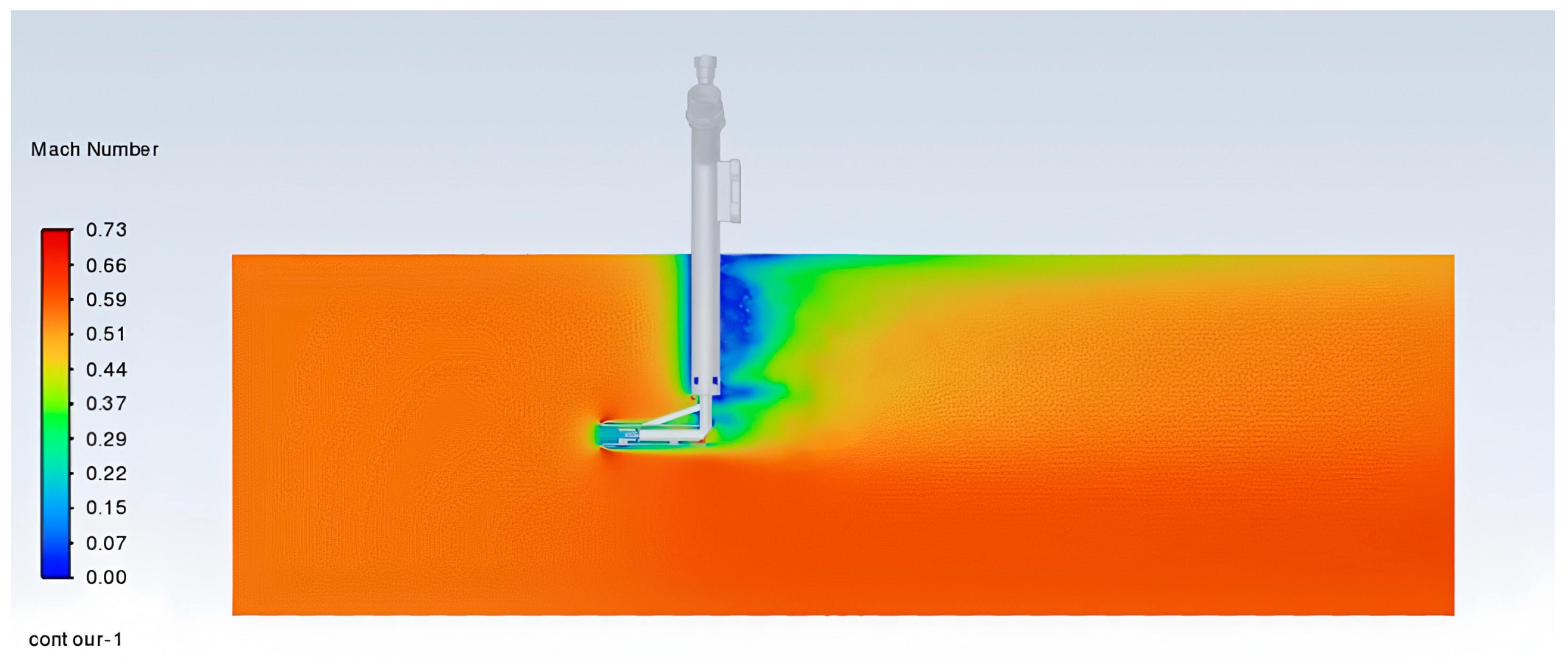
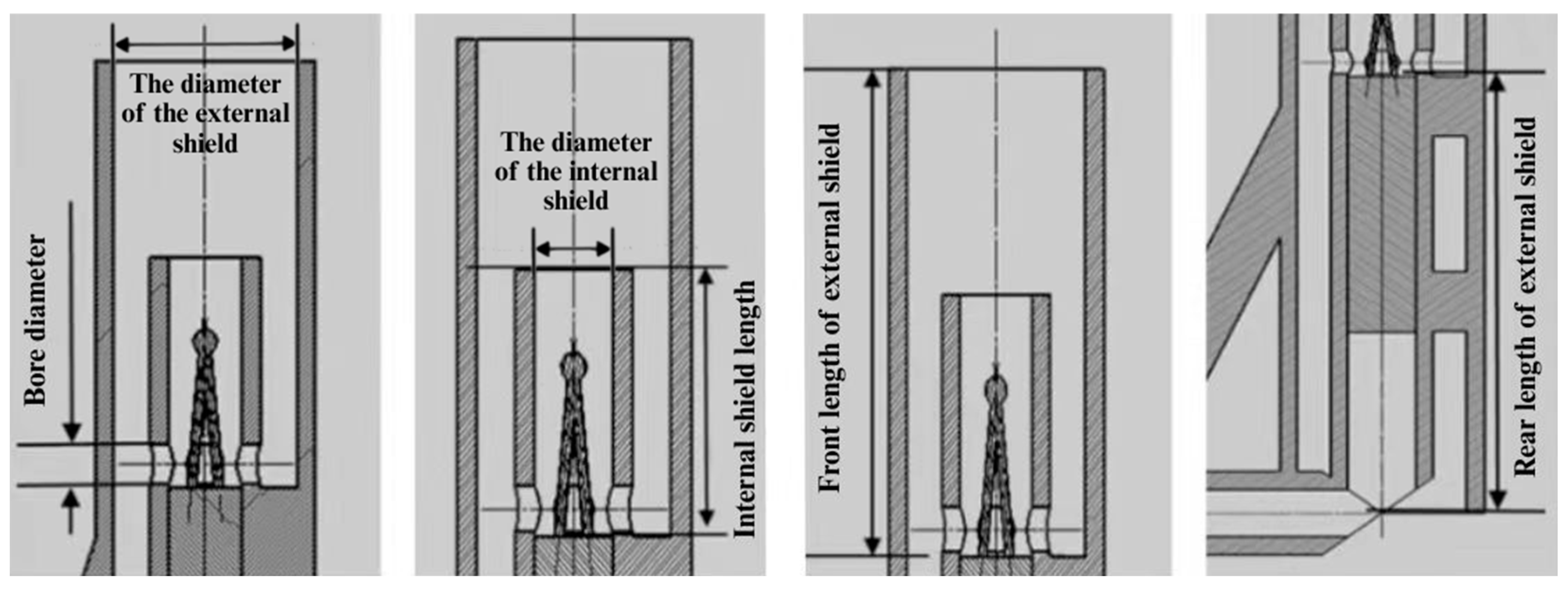
The optimization process aims to minimize the deviation in the total temperature probe’s temperature measurements by adjusting its structural parameters. Given the high-temperature (2300 K), high-pressure (1.0 MPa), and high-Mach number (0.6) operating environment, the primary sources of temperature measurement deviation are conduction and radiation errors. Therefore, the structural parameters selected for optimization are the diameter of the internal shield, the orifice diameter of the internal shield, the diameter of the external shield, the internal shield length, the external shield front length, and the external shield rear length, as shown in the schematic diagram of the optimized parameters in Figure 7. The initial values and ranges of these parameters are presented in

Table 1. Initial values and ranges of variation in the optimized parameters.

Structural Parameters	The Diameter of the Internal Shield $\mathit{D}\mathbf{\text{\_}}\mathit{i}\mathit{n}$ (mm)	Bore Diameter of the Internal Shield $\mathit{D}$ (mm)	The Diameter of the External Shield $\mathit{D}\mathbf{\text{\_}}\mathit{e}\mathit{x}$ (mm)	Internal Shield Length $\mathit{L}\mathbf{\text{\_}}\mathit{i}\mathit{n}$ (mm)	Front Length of External Shield $\mathit{L}\mathbf{\text{\_}}\mathbf{1}$ (mm)	Rear Length of External Shield $\mathit{L}\mathbf{\text{\_}}\mathbf{2}$ (mm)
Initial value	5.00	2.00	11.00	11.60	21.50	36.70
Range of variation	5.0–7.0	1.5–2.5	10.0–12.0	9.6–13.6	18.5–21.5	28.7–36.7

.

This parameter selection is justified by their distinct roles: $D\text{\_}in$ and $D$ collectively determine the inlet-to-outlet area ratio, critically influencing internal flow field structure and recovery characteristics, with literature confirming an optimal ratio exists for minimizing total steady-state error [26]. $D\text{\_}ex$ serves as the primary barrier against high-speed incoming flow, providing flow rectification and deceleration while influencing radiative heat loss. $L\text{\_}in$ governs the internal flow development length and heat conduction path, balancing velocity error reduction against conduction error. $L\text{\_}1$ and $L\text{\_}2$ define the external shield’s geometric configuration, where $L\text{\_}1$ guides incoming flow and affects pressure distribution, while $L\text{\_}2$ governs flow stability and wake effects—together ensuring a stable, low-pressure-loss flow environment for the internal shield.

The objective is to optimize the structure of the total temperature probe by minimizing its temperature measurement deviation. The objective function is established as follows:

$$\begin{gathered} min F\left(D\text{\_}in,D,D\text{\_}ex,L\text{\_}in,L\text{\_}1,L\text{\_}2\right) \\ s.t.\left\{\begin{array}{c}{\displaystyle \genfrac{}{}{0pt}{}{D\text{\_}in\in [ 5.0 , 7.0 ]}{D\in [ 1.5 , 2.5 ]}}\\ {\displaystyle \genfrac{}{}{0pt}{}{D\text{\_}ex\in [ 10.0 , 12.0 ]}{L\text{\_}in\in [ 9.6, 13.6 ]}}\\ {\displaystyle \genfrac{}{}{0pt}{}{L\text{\_}1\in [ 18.5 , 21.5 ]}{L\text{\_}2\in [ 28.7 , 36.7]}}\end{array}\right. \end{gathered}$$

(5)

The temperature-measurement deviation $\Delta T$ is governed by a six-parameter function $F\left(D\text{\_}in,D,D\text{\_}ex,L\text{\_}in,L\text{\_}1,L\text{\_}2\right)$, i.e., $\Delta T=F\left(D\text{\_}in,D,D\text{\_}ex,L\text{\_}in,L\text{\_}1,L\text{\_}2\right)$.

3.1.2. Structural Parameter Analysis

Before constructing the surrogate model and performing optimization, it is essential to quantify the influence of the six key structural parameters on the temperature measurement deviation $\Delta T$ of the total temperature probe and identify their interactions.

To ensure the reliability and robustness of the sensitivity analysis results, global sensitivity analysis based on the Sobol method was conducted using three distinct surrogate modeling approaches: grid-search-optimized SVR, Kriging, and BPNN. This multi-model comparative analysis aims to quantify the influence of the six key structural parameters on the temperature measurement deviation $\Delta T$ and identify their interactions, while verifying the consistency of sensitivity rankings across different modeling techniques.

This study employs three key sensitivity metrics: the first-order index (S1) quantifying individual parameter effects, the total-order index (ST) capturing comprehensive influences including all interactions, and their difference (ST-S1) measuring interaction strength [34].

The first-order sensitivity index ${S1}_i$ measures the direct contribution of the input parameter $X_i$ to the output variance, excluding the interaction effects of this parameter with other parameters. $X_i$ denotes the $i$-th parameter among the six structural parameters. ${S1}_i$ is calculated using the following formula [35]:

$${S1}_i={\displaystyle \frac{V\left[E\left(Y|X_i\right)\right]}{V\left(Y\right)}}$$

(6)

where $V\left[E\left(Y|X_i\right)\right]$ is the variance of the conditional expectation when $X_i$ is fixed. $\mathrm{Y}$ is the true value of the output.

The total-order sensitivity index ${ST}_i$ measures the total contribution of the input parameter $X_i$ to the output variance. The formula for ${ST}_i$ is as follows:

$${ST}_i=1-{\displaystyle \frac{V\left[E\left(Y|X_{~i}\right)\right]}{V\left(Y\right)}}$$

(7)

where $V\left[E\left(Y|X_{~i}\right)\right]$ is the variance of the conditional expectation when other parameters is fixed. $X_{~i}$ is the set of all parameters except $X_i$.

The sensitivity rankings of parameters obtained from the three surrogate models are visually presented in Figure 8, where Figure 8a illustrates the ranking from the SVR model, Figure 8b from the Kriging model, and Figure 8c from the BPNN model. These visual comparisons provide an intuitive understanding of parameter importance across different modeling approaches. The first-order, total-order, and interaction strength Sobol indices obtained from each model are comparatively presented in

Table 2. Comparison of Sobol sensitivity indices from three surrogate models.

Model	Structural Parameter	S1	ST	ST-S1
SVR	$D\text{\_}in$	0.1240	0.3182	0.1942
	$D$	0.0067	0.1444	0.1377
	$D\text{\_}ex$	0.1436	0.3567	0.2130
	$L\text{\_}in$	0.0110	0.1081	0.0970
	$L\text{\_}1$	−0.0047	0.1609	0.1657
	$L\text{\_}2$	0.2605	0.4723	0.2118
Kriging	$D\text{\_}in$	0.1195	0.4059	0.2864
	$D$	0.0045	0.2037	0.1992
	$D\text{\_}ex$	0.1006	0.3702	0.2697
	$L\text{\_}in$	−0.0047	0.1089	0.1136
	$L\text{\_}1$	0.0281	0.2202	0.1921
	$L\text{\_}2$	0.1871	0.4502	0.2630
BPNN	$D\text{\_}in$	0.1289	0.3244	0.1956
	$D$	0.0196	0.1218	0.1022
	$D\text{\_}ex$	0.1425	0.4185	0.2761
	$L\text{\_}in$	0.0223	0.0764	0.0541
	$L\text{\_}1$	−0.0103	0.1490	0.1593
	$L\text{\_}2$	0.2408	0.4926	0.2519

.

The Sobol sensitivity analysis results from the three surrogate models demonstrate good consistency, validating the reliability of the conclusions. As shown in Table 2, all three models identified $L\text{\_}2$ as the most sensitive parameter, with total-order indices (ST) ranging from 0.4502 to 0.4926; $D\text{\_}ex$ and $D\text{\_}in$ ranked as the second and third most sensitive parameters, with ST values ranging from 0.3567 to 0.4185 and 0.3182–0.4059, respectively. Notably, the Kriging model showed slight differences in the ranking of $D\text{\_}in$ and $D\text{\_}ex$ compared to the other two models, but the numerical differences remain within acceptable limits. The interaction strength analysis revealed significant nonlinear coupling effects. All models indicated that $L\text{\_}2$, $D\text{\_}ex$, and $D\text{\_}in$ exhibit the strongest interactions (ST-S1 > 0.19), suggesting complex synergistic or antagonistic effects among these parameters when influencing temperature measurement deviation.

The medium-sensitivity parameters $L\text{\_}1$ and $D$, with ST values in the 0.12–0.22 range, require consideration of their interaction effects with other parameters during optimization. Regarding low-sensitivity parameters, all three models consistently identified $L\text{\_}in$ as having the least influence (ST < 0.12), suggesting it can be assigned lower priority during the optimization process while focusing computational resources on more sensitive parameters.

Overall, the consistency in parameter sensitivity rankings and interaction strength patterns across the three models enhances the credibility of the analysis results, providing a solid theoretical foundation for subsequent probe structure optimization.

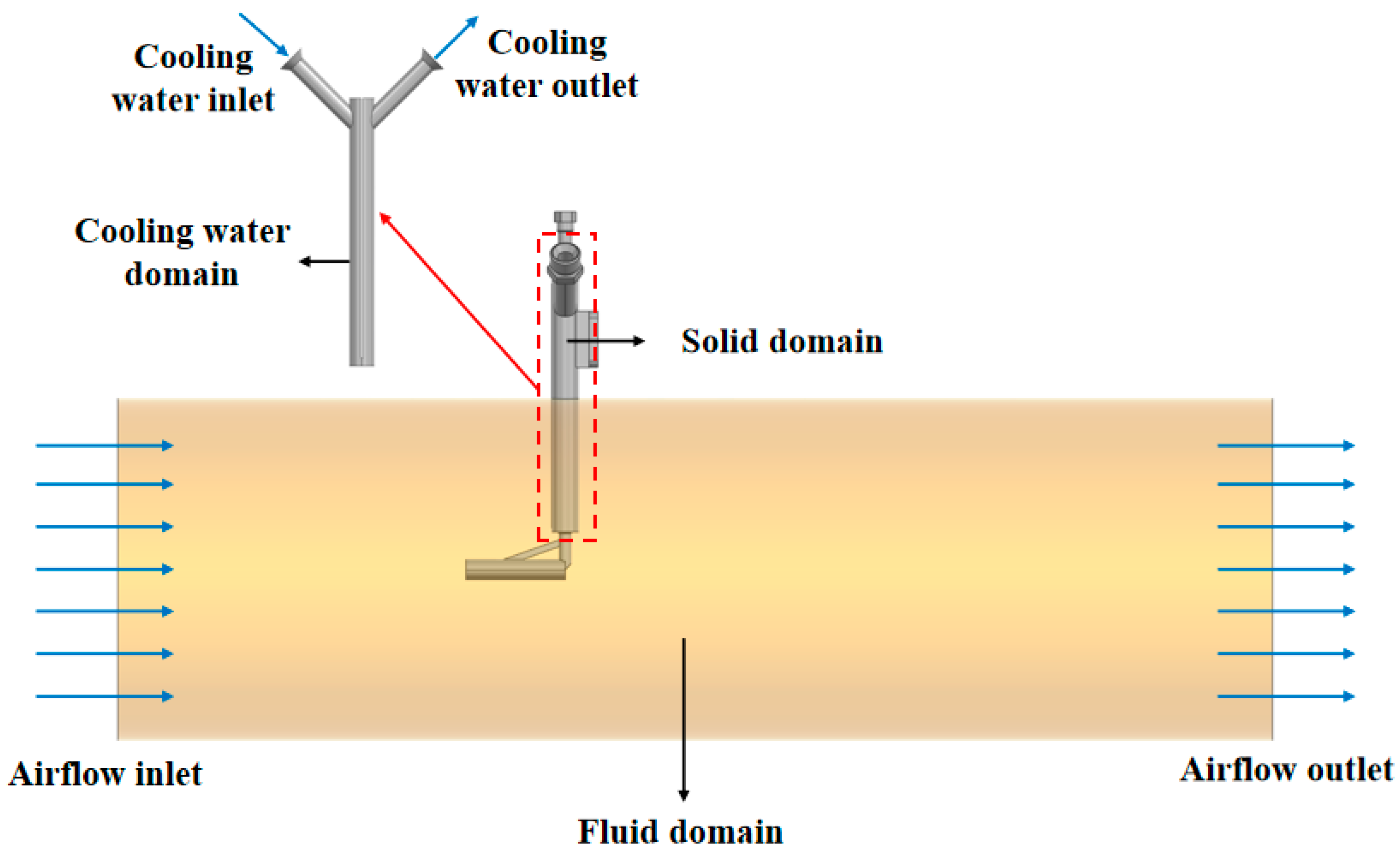
In this paper, the sample data are obtained using the numerical simulation method for the total temperature probe described in Section 2. Under the design conditions of the total temperature probe (inlet total temperature: 2300 K, inlet Mach number: 0.6, environmental pressure: 1.0 MPa), a sensitivity-analysis-based non-uniform sampling strategy was implemented for its six key structural parameters. According to the Sobol sensitivity analysis results, five levels were selected for each of the three highly sensitive parameters ($L\text{\_}2$, $D\text{\_}ex$, $D\text{\_}in$), while three levels were chosen for each of the three less sensitive parameters ($L\text{\_}1$, $D$, $L\text{\_}in$). A full factorial design was employed, generating 3375 representative parameter combinations. For these sampled points, the numerical calculation method described in Section 2, along with Fluent commands, was utilized to individually perform geometric modeling, mesh generation, and numerical simulation. The initial values of the optimization objectives corresponding to the sampled points were obtained by post-processing the simulation results. The sampling strategy, guided by sensitivity analysis, ensures comprehensive coverage of the entire design space while significantly improving the efficiency and focus of data acquisition.

3.2. Surrogate Model

To address the computational challenges associated with high-fidelity numerical simulations, surrogate models have emerged as a powerful tool for efficient optimization and design. These models approximate complex systems with reduced computational cost while maintaining high accuracy. Selecting an appropriate surrogate model is critical. Given that the input is a low-dimensional, structured vector of geometric parameters and the output is a scalar temperature deviation, the problem is well-suited for regression models that excel at learning nonlinear mappings in tabular data. While advanced architectures like Convolutional or Recurrent Neural Networks are powerful for spatial or sequential data, they are not optimized for this type of structured input and may introduce unnecessary complexity. In the context of optimizing the dual-shield total temperature probe for aero-engine applications, a surrogate model based on SVR is employed to predict temperature measurement deviations under varying structural parameters.

We have $N$ data points $X^{\left(i\right)}=\left[{D_{in}}^{\left(i\right)},D^{\left(i\right)},{D_{ex}}^{\left(i\right)},{L_{in}}^{\left(i\right)},{L_1}^{\left(i\right)},{L_2}^{\left(i\right)}\right], i=\mathrm{1,2}, \dots , N$ and their corresponding outputs $y^{\left(i\right)}$, the objective is to predict the output $\widehat{y}\left(X^{\left(new\right)}\right)$ for a new input point $X^{\left(new\right)}=[D\text{\_}in,D,D\text{\_}ex,L\text{\_}in,L\text{\_}1,L\text{\_}2]$.

SVR seeks to identify a hyperplane that best fits the training data while minimizing prediction error. Unlike methods that require minimizing errors for all sample points, it employs a loss function known as the $\epsilon$-insensitive loss function. This function does not penalize prediction errors smaller than $\epsilon$, while applying linear penalties only to deviations exceeding this threshold. Such a design enhances the model’s robustness. The loss function is formally defined as follows:

$$L\left(y^{\left(i\right)},{\widehat{y}}^{\left(i\right)}\right)=\left\{\begin{array}{l}0 if \left|y^{\left(i\right)}-{\widehat{y}}^{\left(i\right)}\right|\le \epsilon \\ \left|y^{\left(i\right)}-{\widehat{y}}^{\left(i\right)}\right|-\epsilon otherwise\end{array}\right.$$

(8)

where $y^{\left(i\right)}$ is the true value, ${\widehat{y}}^{\left(i\right)}$ is the predicted value. This equation indicates that loss is calculated only when the difference between the predicted and actual values exceeds $\epsilon$. When the error exceeds $\epsilon$, the loss becomes proportional to the amount by which it exceeds this threshold.

The mathematical model of SVR can be expressed as the following optimization problem:

$$\underset{\omega ,b,\xi ,{\xi }^{*}}{\mathit{min}}\left({\displaystyle \frac{1}{2}}{‖\mathit{\omega }‖}^2+C{\sum }_{i=1}^N\left({\xi }_i+{\xi }_i^{*}\right)\right)$$

(9)

where $\mathit{\omega }$ is the weight vector representing model complexity. ${\xi }_{\mathrm{i}}$ and ${\xi }_{\mathrm{i}}^{\mathrm{*}}$ are slack variables used to handle data points that cannot be fitted precisely. $C$ is the regularization parameter that controls the trade-off between model complexity and error, also referred to as the penalty parameter. A larger $C$ imposes a heavier penalty on points lying outside the margin band, causing the model to attempt to fit more data points; conversely, a smaller $C$ results in higher tolerance for errors.

The constraints for SVR are as follows:

$$\left\{\begin{array}{c}{y}^{\left(i\right)}-\left({\mathit{\omega }}^T{X}^{\left(i\right)}+b\right)\le \epsilon +{\xi }_i,\\ \left({\mathit{\omega }}^T{X}^{\left(i\right)}+b\right)-y^{\left(i\right)}\le \epsilon +{\xi }_i^{*},\\ {\xi }_i,{\xi }_i^{*}\ge 0 i=1,\dots ,N\end{array}\right.$$

(10)

where $b$ is the bias term. These constraints ensure that the model’s prediction errors do not exceed $\epsilon$, and they allow for some flexibility through the slack variables to handle data points that are difficult to fit precisely.

SVR employs a kernel function to map the input data into a high-dimensional space, enabling the identification of a linear hyperplane for fitting the data in this space. Commonly used kernel functions include linear, polynomial, and radial basis function (RBF) kernels. The RBF kernel function $K(X^{\left(i\right)},X^{\left(j\right)})$ is defined as:

$$K(X^{\left(i\right)},X^{\left(j\right)})={\Phi \left(X^{\left(i\right)}\right)}^T·\Phi \left(X^{\left(j\right)}\right)=exp\left(-\gamma {‖X^{\left(i\right)}-X^{\left(j\right)}‖}^2\right)$$

(11)

where $\Phi \left(X^{\left(i\right)}\right)$ is the high-dimensional mapping of the input vector $X^{\left(i\right)}$, the parameter $\gamma$ controls the shape of the kernel function.

By solving the dual problem of Equation (9), the optimal Lagrange multipliers ${{\alpha }_i,\alpha }_i^{*}$ can be obtained. Subsequently, $\mathit{\omega }$ and $b$ are calculated. Finally, the prediction for a new input point $X^{\left(new\right)}$ is:

$$\widehat{y}\left(X^{\left(new\right)}\right)={\sum }_{i=1}^N\left({\alpha }_i-{\alpha }_i^{*}\right)K(X^{\left(i\right)},X^{\left(new\right)})+b$$

(12)

3.3. Genetic Algorithm Optimization

To efficiently identify the global optimal configuration of the probe’s structural parameters for minimizing temperature measurement deviation, a GA was employed. GAs are a class of population-based optimization techniques inspired by the principle of natural evolution, renowned for their robustness in handling nonlinear, high-dimensional problems and their strong global search capability without requiring gradient information. This makes them particularly suitable for the present study, where the trained SVR surrogate model implicitly defines the objective function.

The selection of the Genetic Algorithm for this optimization task was motivated by several key factors that align with the problem’s characteristics. Firstly, the relationship between the six structural parameters and the temperature deviation is highly nonlinear and expected to be multimodal, presenting a complex design space. GA, as a population-based global search method, is particularly adept at exploring such spaces without being trapped in local optima, a common pitfall of gradient-based algorithms. Secondly, GA operates without requiring derivative information, which is advantageous when the objective function is implicitly defined by a surrogate model, as in this study. Lastly, GA has a well-established track record of successful integration with surrogate models for the optimization of complex engineering systems, including thermal management [25,28], electromechanical design [26,29], and fluidic systems [27], providing a reliable and validated foundation for our approach.

A GA is used to optimize the probe’s structural parameters to minimize the temperature measurement deviation of total temperature probe. These parameters include inner screen aperture diameter, inner screen length, external shield front length, and external shield rear length. The optimization problem can be described as follows.

$$\begin{gathered} \underset{X}{\mathit{min}}\left|T_{mean}\left(X\right)-T_{true}\right| \\ s.t. {\sigma }_{T, weighted}=\sqrt{{\displaystyle \frac{{\sum }_{i=1}^n{A}_i{\left(T_i-T_{mean}\left(X\right)\right)}^2}{{\sum }_{i=1}^n{A}_i}}}<1 \end{gathered}$$

(13)

In the formula, $X$ is the vector of structural parameters ${[D\text{\_}in,D,D\text{\_}ex,L\text{\_}in,L\text{\_}1,L\text{\_}2]}^T$. $T_{mean}$ is the probe’s measured value from the simulation, which corresponds to the true output value $y^{\left(i\right)}$ for that data point. $T_{true}$ is the true total temperature (2300 K). In the constraint formula, ${\sigma }_{T, weighted}$ is the standard deviation of the surface Weighted temperature. $n$ is the number of grid points on the thermocouple bead surface, which is 1426 in this study. $T_i$ is the temperature at the $i$-th surface cell. $A_i$ is the area of the $i$-th cell. ${\sum }_{i=1}^N{A}_i$ is the total surface area.

${\sigma }_{T, weighted}$ directly quantifies the absolute dispersion of the local temperature from the mean value. A smaller ${\sigma }_{T, weighted}$ indicates a more uniform temperature field with smaller thermal gradients.

Imposing a constraint ${\sigma }_{T, weighted}$ guides the optimization away from designs that might have a good average temperature but suffer from severe local hot spots or cold spots. A uniform temperature distribution on the sensing element leads to a more stable and reliable measurement signal by minimizing errors induced by internal heat conduction.

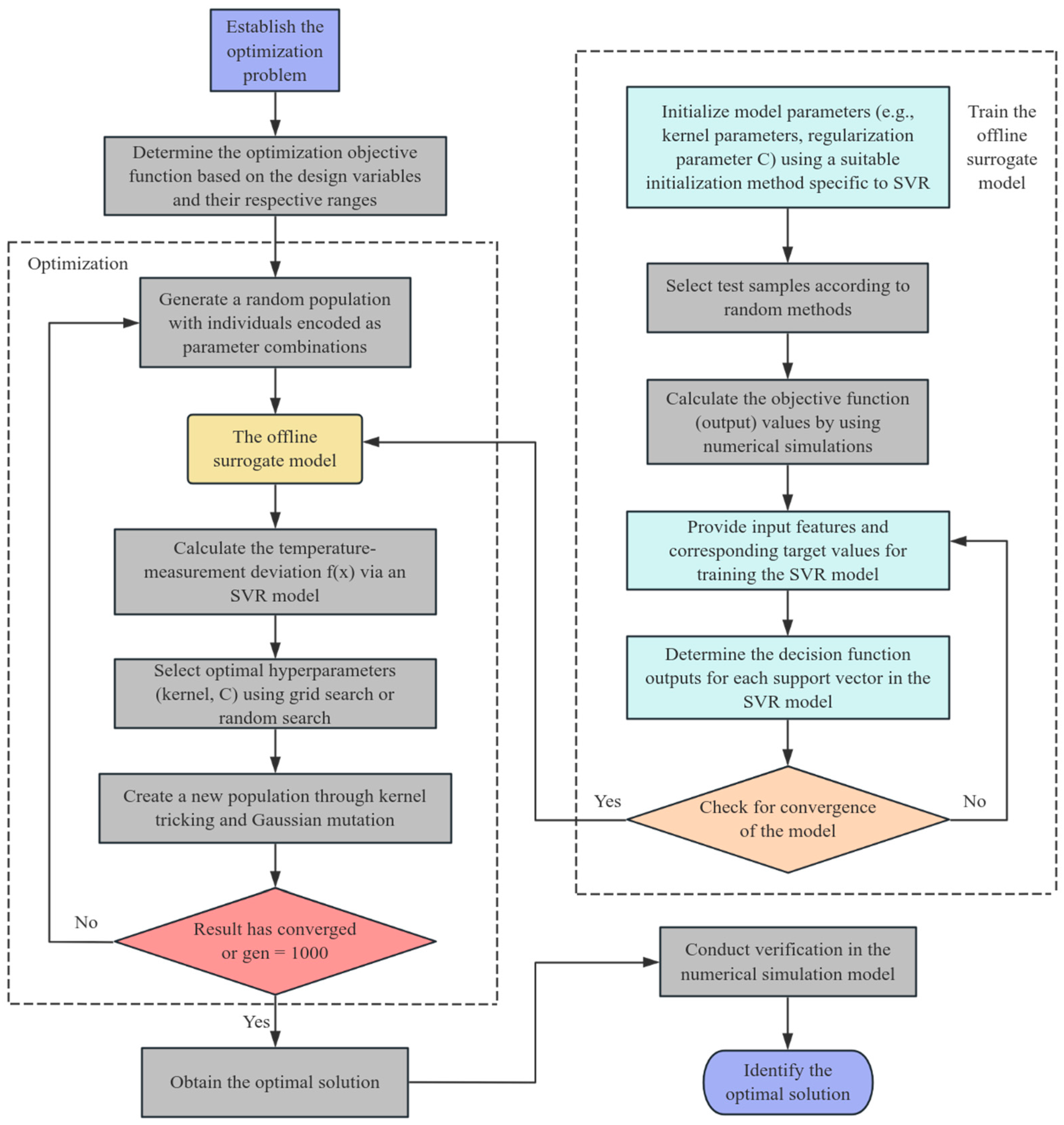
As shown in Figure 9, the optimization of the total temperature probe follows these steps:

The GA was configured with careful consideration to balance exploration of the design space and convergence efficiency. The fitness function was defined as the temperature measurement deviation determined by six key structural parameters, which was approximated using the SVR surrogate model to replace computationally expensive high-fidelity simulations. A population size of 500 individuals was chosen to maintain sufficient genetic diversity. The algorithm used a blend crossover with a probability of 0.9 to recombine promising solutions, and a Gaussian mutation operator with a probability of 0.1 to introduce perturbations and prevent premature convergence. The optimization process was set to terminate after 1000 generations, with elitism used to preserve the best solution across generations.

3.4. Simulation Verification

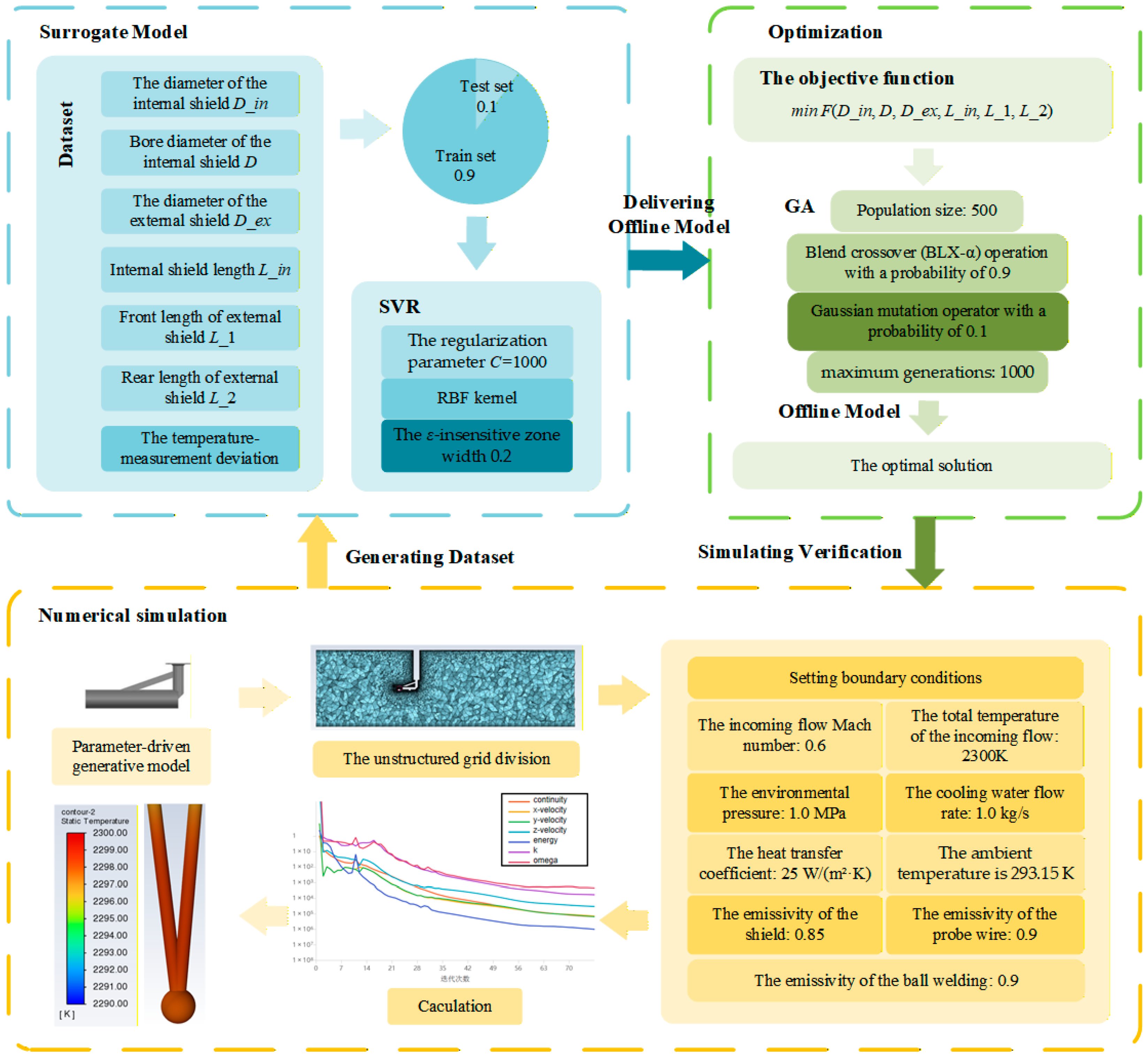
To clearly demonstrate the implementation process of the simulation verification and its position within the overall optimization framework, the comprehensive workflow is depicted in Figure 10. This verification step essentially executes the “Numerical simulation” branch of the framework, utilizing the optimal structural parameters obtained from the “Offline Model”.

The specific implementation follows the detailed settings outlined in the diagram: an unstructured grid was employed for meshing, and the boundary conditions were applied. This high-fidelity simulation, conducted under the same rigorous conditions used to generate the training dataset, serves as the definitive benchmark for validating the surrogate model’s predictive accuracy and the genetic algorithm’s optimal solution.

3.4.1. Surrogate Model Construction

The dataset was divided into training and test sets at a ratio of 9:1. The optimal parameters for the SVR model were determined through a comprehensive grid search process, considering various combinations of regularization parameter $C$, kernel parameter $\gamma$, and $\epsilon$-insensitive zone width. The final SVR model in this study employs an RBF kernel, with the regularization parameter $C$ set to 1000, the kernel parameter $\gamma$ set to 1, and the $\epsilon$-insensitive zone width set to 0.2. These parameters are chosen to balance model complexity and predictive accuracy.

The parameter $C$ controls the trade-off between the model’s complexity and its ability to fit the training data. A smaller $C$ value results in a simpler model that allows for larger errors, potentially leading to underfitting. Conversely, a larger $C$ value results in a more complex model that fits the training data more precisely, potentially leading to overfitting. In this study, $C$ is set to 1000 to ensure a high level of model complexity and precise fitting of the training data.

The kernel parameter $\gamma$ controls the width of the RBF kernel. A smaller $\gamma$ value indicates a wider kernel, making the model less sensitive to local variations and more suitable for capturing global trends. A larger $\gamma$ value indicates a narrower kernel, making the model more sensitive to local variations and better suited for capturing local features. In this study, $\gamma$ is set to 1 to balance sensitivity to local and global variations in the data.

The $\epsilon$-insensitive zone width $\epsilon$ defines the model’s tolerance for errors. A smaller $\epsilon$ value makes the model more sensitive to errors, allowing fewer errors and thus increasing the model’s complexity. A larger $\epsilon$ value makes the model less sensitive to errors, allowing more errors and thus reducing the model’s complexity. In this study, $\epsilon$ is set to 0.2 to provide a moderate level of error tolerance, ensuring that the model is neither overly complex nor overly simplified.

To demonstrate the advantages of the SVR model as a surrogate model for this problem, we additionally employed Kriging and BPNN as surrogate models to approximate the target problem. The performance of these three models was evaluated under their respective optimal parameter configurations.

The relevant parameters of the Kriging model were configured as follows: the initial parameter $\theta$ was set to 0.01 to control the kernel width and balance sensitivity to local variations against overfitting risks; the squared exponential kernel function was selected for its suitability to smooth data; and a nugget parameter $\delta$ of 1 × 10⁻¹² was applied to enhance numerical stability while preventing underfitting from excessive regularization.

The relevant parameters of the BPNN model were configured as follows: the input layer consists of 6 nodes; there are two hidden layers, the first with 128 nodes and the second with 64 nodes, both using the ReLU activation function; the output layer has one node with a linear activation function; the Adam optimizer was adopted with a learning rate of 0.02; the training was run for 2000 epochs with a batch size of 20, and the verbose setting was set to 1.

The model evaluation metric uses the coefficient of determination, $R^2$, which ranges from 0 to 1. A value closer to 1 indicates better model performance, while a value closer to 0 suggests worse performance. The formula is as follows:

$$R^2=1-{\displaystyle \frac{\sum _{i=1}^N{\left(y^{\left(i\right)}-{\widehat{y}}^{\left(i\right)}\right)}^2}{\sum _{i=1}^N{\left(y^{\left(i\right)}-\overline{y}\right)}^2}}$$

(14)

where ${\widehat{y}}^{\left(i\right)}\left(i=\mathrm{1,2},\dots ,N\right)$ is the predicted value for the i-th sample, $y^{\left(i\right)}\left(i=\mathrm{1,2},\dots ,N\right)$ is the actual value for the $i$-th sample, $\overline{y}$ is the average value of the actual value, and $N$ is the number of samples.

The prediction results of the three models are shown in Figure 11, where Figure 11a presents the SVR model’s performance, Figure 11b shows the Kriging model’s performance, and Figure 11c displays the BPNN model’s results.

The SVR model achieved an $R^2$ value of 0.9591 and a Mean Squared Error (MSE) of 3.3869; the Kriging model attained an $R^2$ of 0.9086 and an MSE of 2.1594; while the BPNN model yielded an $R^2$ of 0.7881 and an MSE of 10.8098, as shown in

Table 3. Comparative Performance of Three Surrogate Models.

Evaluation Metrics	The SVR Model	The Kriging Model	The BPNN Model
$R^2$	0.9591	0.9086	0.7881
MSE	3.3869	2.1594	10.8098

.

In terms of $R^2$, the SVR model significantly outperforms both Kriging and BPNN. As evidenced in Figure 11, the deviations between the predicted and actual values are notably smaller for the SVR model. Therefore, the SVR model is more suitable for the problem under investigation.

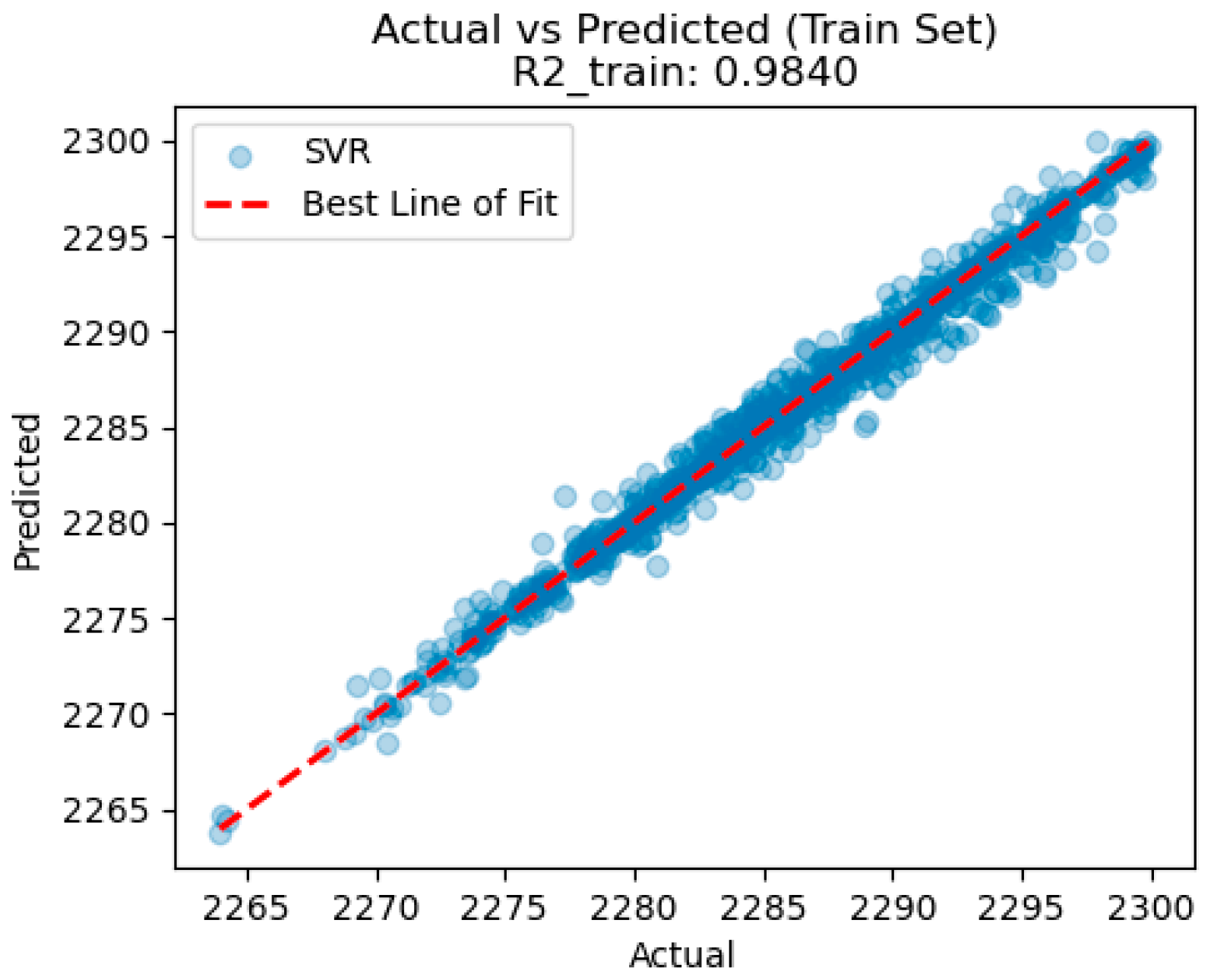
The complete training results of the SVR model are presented below. Figure 12 illustrates the model performance on the training set, where the $R^2$ is 0.9840 and the MSE is 0.7220. These metrics indicate that the model fits the training data very well. The low MSE value further suggests that the model’s predictions are close to the actual values, with minimal deviation.

Figure 11a presents the model performance on the testing set, with an $R^2$ of 0.9503 and an MSE of 3.3869. The slightly lower $R^2$ value and higher MSE on the test set compared to the training set suggest that, while the model generalizes well to unseen data, it shows a modest increase in prediction error. This is expected, as models often perform better on training data due to overfitting.

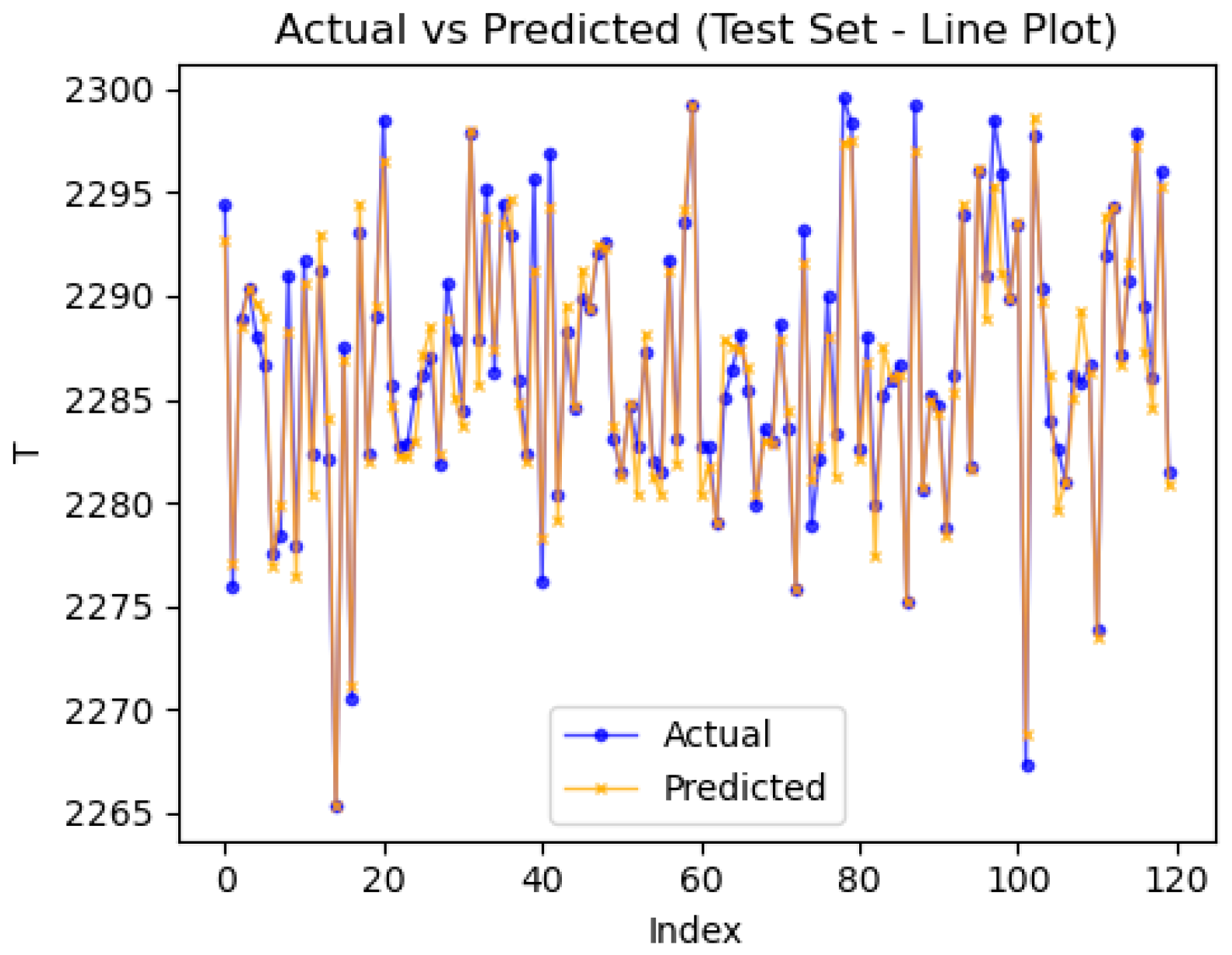
Figure 13 compares prediction results. This suggests the SVR is suitable as a surrogate model for genetic algorithm optimization in this paper.

3.4.2. Verification of Optimization Results

In Section 3.3, we discussed the basic optimization workflow and detailed the genetic algorithm’s parameter settings. In this section, we validate the optimization results to demonstrate the feasibility of the proposed methodology.

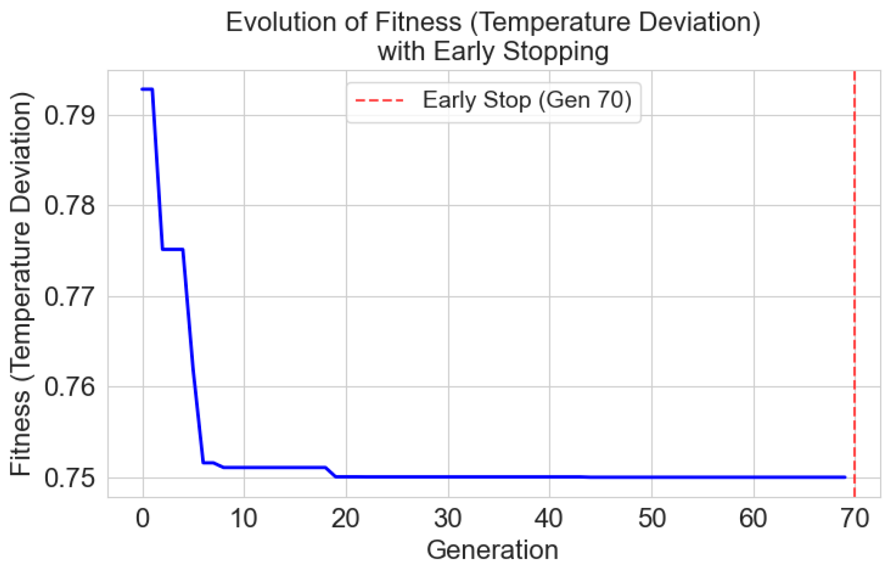
The convergence behavior of the Genetic Algorithm, monitored through the evolution of the objective function (temperature deviation $\Delta T$), is presented in Figure 14. The history shows a characteristic trend: a rapid and substantial decrease in $\Delta T$ during the initial 20 generations, as the algorithm efficiently explores the design space and identifies promising regions. This is followed by a period of refined search with diminishing returns, where only minor improvements are achieved. The population reached a stable global optimum around the 70th generation, with no further significant improvement observed thereafter.

The optimal set of structural parameters identified by the GA is listed in

Table 4. Comparison of structural parameter dimensions before and after.

Structural Parameters	The Diameter of the Internal Shield $\mathit{D}\mathbf{\text{\_}}\mathit{i}\mathit{n}$ (mm)	Bore Diameter of Internal Shield $\mathit{D}$ (mm)	The Diameter of the Internal Shield $\mathit{D}\mathbf{\text{\_}}\mathit{e}\mathit{x}$ (mm)	Internal Shield Length $\mathit{L}\mathbf{\text{\_}}\mathit{i}\mathit{n}$ (mm)	Front Length of External Shield $\mathit{L}\mathbf{\text{\_}}\mathbf{1}$ (mm)	Rear Length of External Shield $\mathit{L}\mathbf{\text{\_}}\mathbf{2}$ (mm)
Before	5.00	2.00	11.00	11.60	21.50	36.70
After	5.90	2.07	11.92	11.77	20.36	35.39

. The temperature measurement deviation was reduced from an initial value of 2.05 K to an optimal value of 0.75 K, corresponding to a reduction of 1.30 K.

The optimization results are both physically meaningful and align with the earlier sensitivity analysis. The most significant adjustments occurred in the most sensitive parameters: a reduction in the rear shield length ($L\text{\_}2$) to stabilize the wake flow, and an increase in the shield diameters ($D\text{\_}in$, $D\text{\_}ex$) to enhance radiative shielding and flow recovery. These synergistic changes effectively balance the reduction in velocity, conduction, and radiation errors.

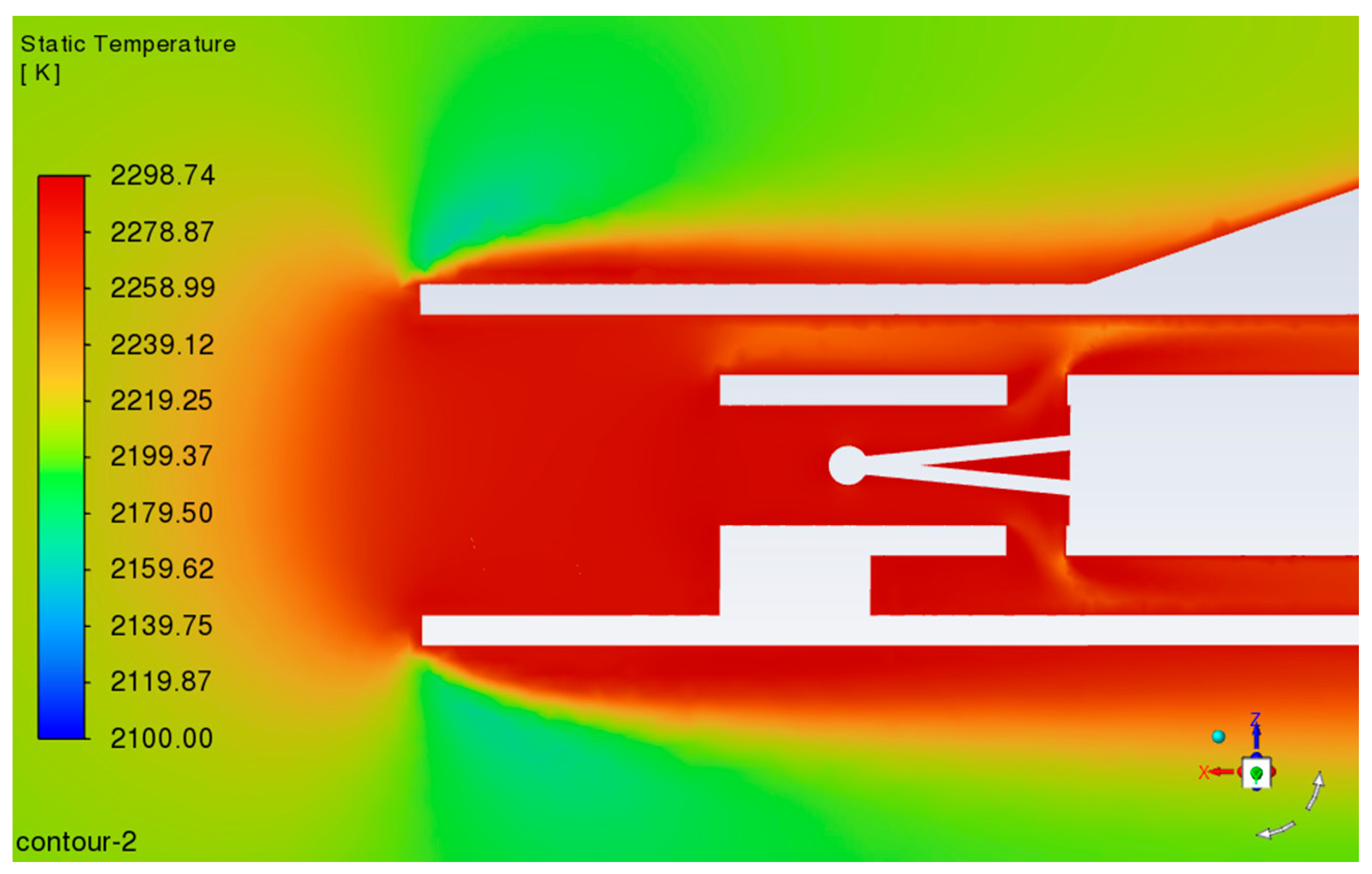
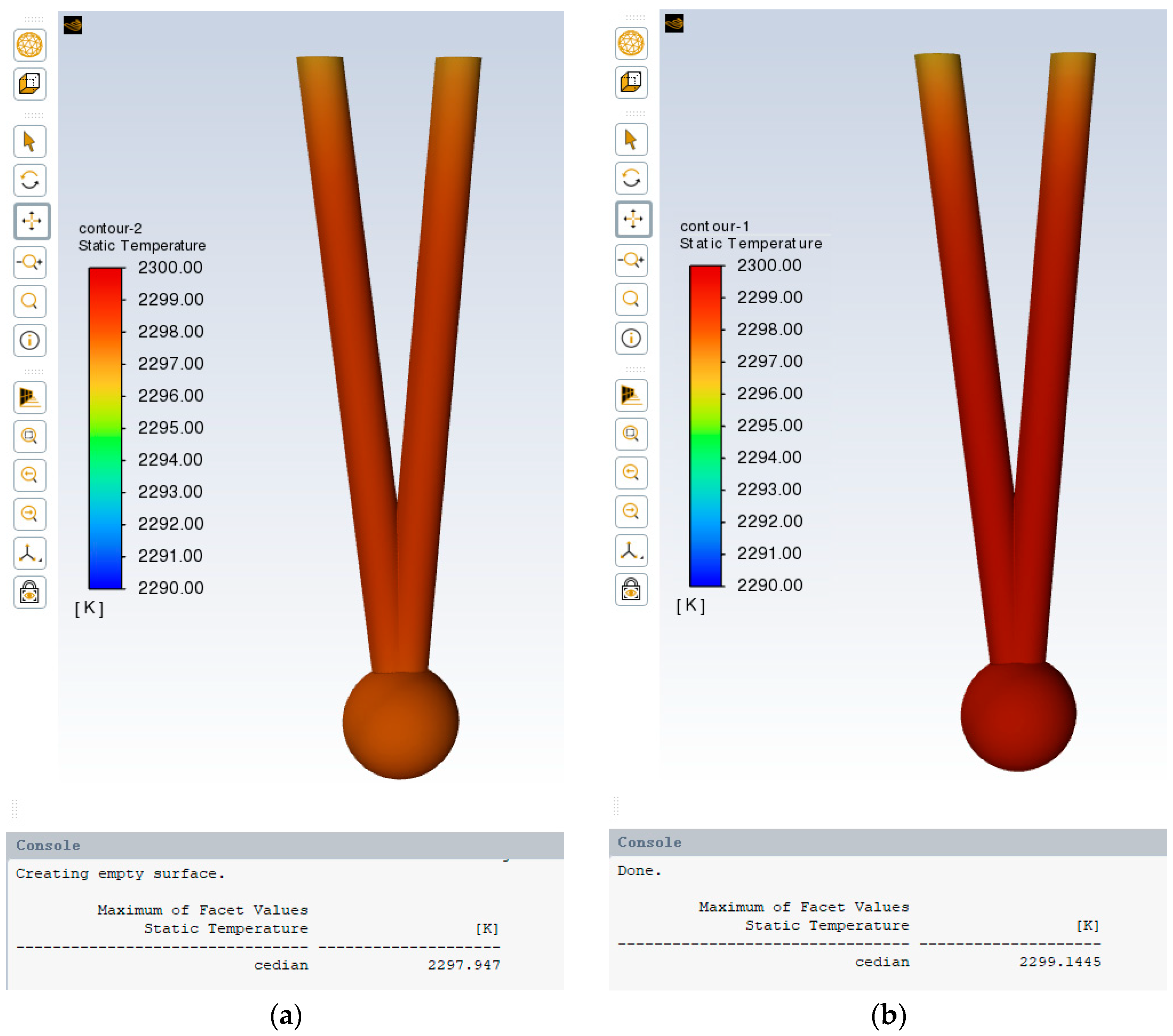
Under representative aero-engine operating conditions (total temperature: 2300 K, Mach number: 0.6, pressure: 1.0 MPa), the probe was redesigned in 3D using optimized structural parameters to verify its measurement accuracy. After extracting the computational domain, meshing, and setting the boundary conditions, high-fidelity simulations were conducted to obtain detailed temperature distributions. 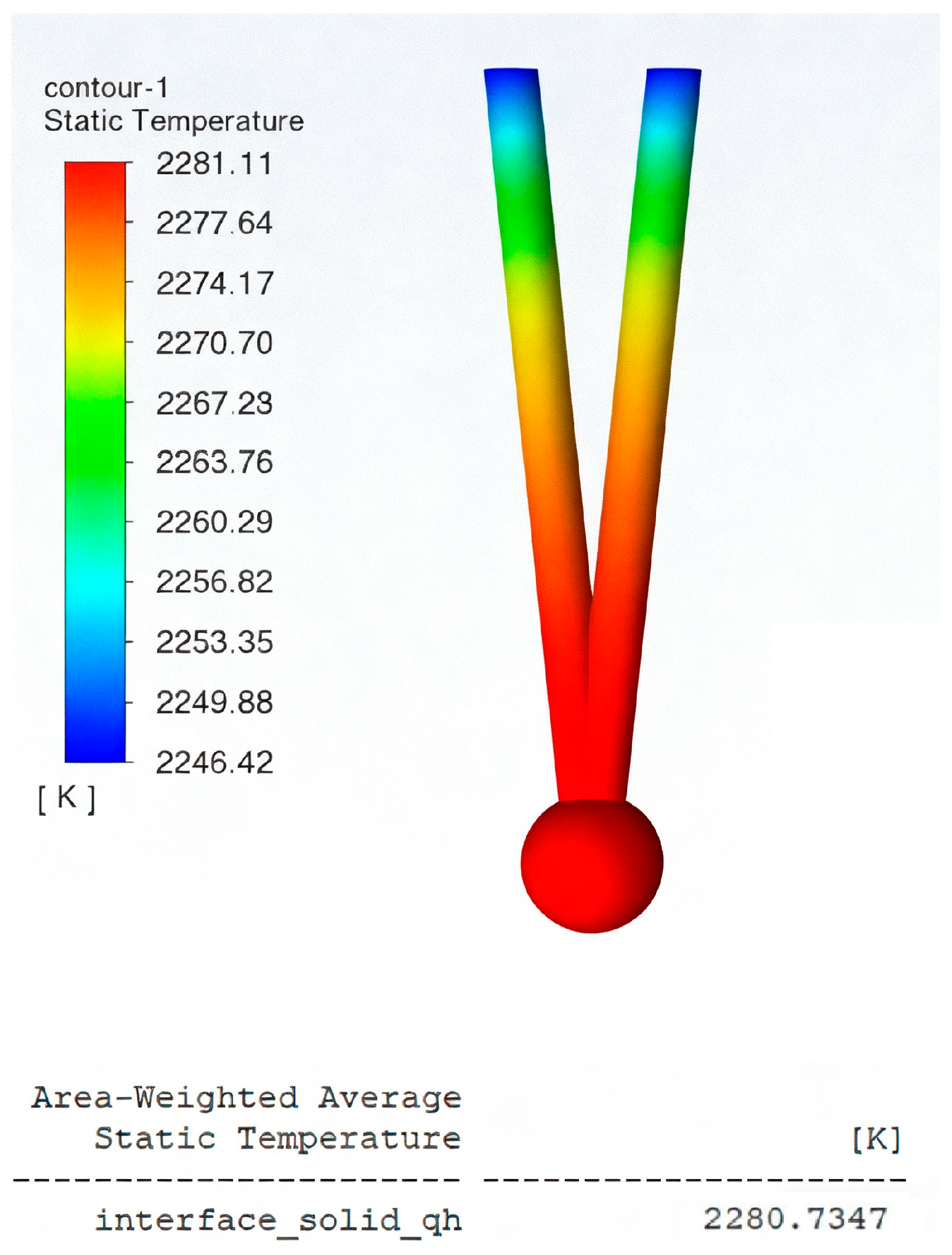Figure 15a presents the simulation results for the initial design, showing a temperature deviation of 2.05 K. In contrast, the optimized probe in Figure 15b exhibits a significantly reduced deviation of approximately 0.86 K. This performance meets the stringent accuracy requirements (typically within ±1.0 K) for high-precision temperature measurement in critical aero-engine applications. Furthermore, the absolute error between this validated result and the genetic-algorithm-predicted value (0.75 K) is only 0.11 K, demonstrating the high predictive accuracy of the surrogate model-based optimization framework and its ability to meet rigorous engineering design goals.

4. Conclusions

This study developed and validated an automated optimization framework integrating conjugate heat transfer CFD, Support Vector Regression surrogate modeling, and a Genetic Algorithm for the design of a dual-shield total temperature probe for aero-engine applications.

The framework effectively solves the problems of traditional design methods reliant on costly experimentation or high-fidelity simulation loops. The application of the proposed framework successfully reduced the probe’s temperature measurement deviation from an initial 2.05 K to an optimized value of 0.86 K. This represents an absolute reduction of 1.19 K and a 58% relative improvement in accuracy. The optimized design meets the stringent ±1.0 K accuracy requirement for critical aero-engine total temperature measurements.

The core workflow of the developed framework is geometry-agnostic. It provides a cost-effective and generalizable strategy that can be readily adapted to the optimized design of various other temperature sensors, pressure probes, and similar aerothermodynamic components across a wide range of operating conditions, making way for high-performance, low-cost, and rapid development cycles for advanced equipment.

Despite these promising results, certain limitations remain. Firstly, the current surrogate model is constructed for a fixed set of inflow conditions. Future work will incorporate inflow Mach number, total temperature, and pressure as additional input variables to develop a condition-agnostic design tool with stronger generalization capabilities. Secondly, as problem complexity increases, both surrogate modeling and optimization methods need enhancement. We plan to explore deep learning-based modeling approaches and more advanced optimization algorithms like PSO or SSO to solve more challenging design problems. Finally, physical experimentation remains essential for validation. Our next step is to manufacture the optimized probe and conduct calibration tests in a high-temperature wind tunnel, closing the loop between digital design and physical implementation.