Efficient Meshless Phase-Field Modeling of Crack Propagation by Using Adaptive Load Increments and Variable Node Densities

Abstract

This study employs the fourth-order phase-field method (PFM) to investigate crack propagation. The PFM incurs significant computational costs due to its need for a highly dense node arrangement for accurate crack propagation. This study proposes an adaptive loading step size strategy combined with a scattered node (SCN_var) arrangement with variable spacings. The mechanical and phase-field models are solved using the strong-form meshless local radial basis function collocation method in a staggered approach. The method’s performance is evaluated based on accuracy and computational cost, using regular nodes (RGN) and scattered nodes (SCN_uni) with uniform spacing, as well as SCN_var with variable node spacing. Two benchmark tests are used to analyze the proposed method: a symmetric double-notch tension and a single-edge notch shear test. The analysis shows that the adaptive step size strategy improves numerical stability while the SCN_var significantly reduces computational cost. Using SCN_var, the CPU time is decreased by about thirty times compared to uniform nodes in the tensile case and by approximately three times in the shear case, without sacrificing accuracy. This confirms that directing computational resources to critical regions can significantly reduce CPU time, suggesting that adaptive node redistribution could further enhance computational performance.

1. Introduction

One of the significant problems in structural engineering is the initiation and propagation of cracks, which affects durability, service life, and human safety. Established methods like Griffith’s theory [1] and linear elastic fracture mechanics (LEFM) [2] provide the basic concepts for crack initiation and propagation. Still, they fail when dealing with intricate processes such as crack initiation, nucleation, and branching [3]. To address the limitations of conventional methods, the phase-field method (PFM) emerged approximately two decades ago and has gained considerable popularity in modeling crack initiation and propagation. In the PFM, instead of a discrete discontinuity, the cracks are represented diffusely by a scalar phase-field (PF) parameter $\varphi$ [4,5,6]. This PF parameter transitions from a completely intact ($\varphi =0$) to a completely fractured material ($\varphi =1$), thereby eliminating the necessity for explicit tracing of the crack propagation.

The PFM is used for simulating fracture phenomena in research and practical applications [7], enabling the prediction of various phenomena, such as crack coalescence [8] and branching [6] under diverse loading conditions. This method was first introduced by Bourdin et al. [9] in the late 1990s by considering the variational form of Griffith’s theory, which was numerically implemented in 2000 [5]. The method was then further extended by Miehe et al. [10,11] in 2010, considering a thermodynamically consistent crack field. This extension of the PFM has opened numerous applications for tackling fracture analysis in brittle and ductile materials subjected to pure mechanical [12,13,14,15] or thermomechanical [8,16] loading conditions. Although the PFM is still in the development phase, it has been applied to simulate intricate crack phenomena, including fatigue [17,18], dynamic [6,19], and anisotropic [20,21,22] crack propagation, as well as hydrogen-assisted [7,18] cracking. Despite its significant success, the PFM still suffers from its high computational cost. It requires a fine mesh density and small loading increments for accurate crack propagation [23,24].

The finite element method (FEM) is widely used because of its well-established and commercially available software for crack propagation using PFM. FEM has the advantage of utilizing adaptive meshing strategies efficiently, which can significantly reduce computational cost [25,26]. Still, creating and refining the best possible mesh in certain areas can pose a significant challenge in scenarios involving three-dimensional problems, irregular geometries, and multiple cracks evolving simultaneously. Meshless methods have gained increasing popularity due to their capability to handle complex geometries and evolving discontinuities without dependence on element connectivity [27,28,29]. The complex variable element-free Galerkin method [29] and the complex variable moving least-squares approximation [30] offer a potential alternative for modeling complex problems, such as 3D elastoplastic and fracture analysis. Specifically, in fracture problems, the complex least-squares approximation mitigates ill-conditioning, providing high accuracy and efficient computation. The local radial basis function collocation method (LRBFCM) offers high accuracy and is particularly suitable for strong-form discretizations of partial differential equations, as demonstrated by recent studies [8,31,32,33]. The LRBFCM has been successful in solving heat diffusion [32], thermoelasticity [34], PF formulated dendritic growth [31], and elasto-plastic [35] problems. Additionally, the authors have developed and validated a meshless PFM for brittle fracture under various loading conditions [8,24,36], thereby demonstrating its potential as a robust alternative to FEM in fracture analysis.

While meshless methods help to mitigate certain geometric limitations of FEM, they are still computationally demanding because a fine spatial resolution is required for both displacement and PF variables. To reduce this cost, various adaptive strategies have been proposed, including adaptive mesh refinement [37,38], adaptive time-stepping [39], and error-driven spatial adaptivity [40]. Although adaptive mesh-refinement is well-established in FEM, creating efficient adaptive schemes for meshless methods remains an active area of research. Notably, there is a lack of systematic studies on integrating adaptive loading step sizes with variable node densities in meshless PF simulations. The adaptive time-stepping introduced in [39] works by using an error indicator that is based on both the PF and the history field variables. These methods have proven effective, but they require the simultaneous evaluation and monitoring of multiple variables. This study introduces a simpler, more efficient process, where the loading step size is adaptively controlled solely based on the PF variable.

The concept of variable node density offers an attractive approach to strike a balance between accuracy and efficiency. Refining discretization solely along the expected crack path while using coarser nodes elsewhere can significantly decrease computational effort without compromising accuracy. Several FEM studies have examined similar ideas using adaptive meshing and enrichment techniques [37,41,42,43,44,45]. However, in meshless methodologies, the application of predetermined variable node densities, where refinement is prescribed in advance based on anticipated crack trajectories, has not been thoroughly investigated in relation to traditional fracture benchmarks. Furthermore, the interaction between variable node density and adaptive load stepping, which modulates the incremental load step size according to crack progression, remains largely unexamined.

This paper comprehensively addresses these gaps through a systematic analysis of meshless PF fracture simulations, employing two well-established benchmark tests: the Single-Edge Notch Shear (SENS) test and the Symmetric Double-Notch Tension (SDNT) test. These benchmark problems are frequently used in scholarly literature to validate fracture models, as their crack propagation and load–displacement behavior are well-documented [12,46]. Three approaches are examined: (i) uniform node density with non-adaptive load stepping, (ii) uniform node density with adaptive load stepping, and (iii) variable node density with adaptive load stepping. The results are evaluated based on the prediction of crack propagation, force–displacement behavior, and computational efficiency. Particular emphasis is placed on minimizing computation time by integrating adaptive stepping and variable node density.

The paper is divided into different sections. Section 2 explains the governing equations of the fourth-order PF formulation, the strong-form meshless method, and its application in the solution procedure. It also describes the adaptive loading increment size and the approach for creating variable node density distributions. Section 3 presents the benchmark test cases and offers an overview of the numerical results. Finally, Section 4 highlights the main findings and proposes future research directions.

2. Governing Equations and Numerical Method

The governing equations for the PF and mechanical models are derived from the minimization of the total energy functional [36] with respect to displacement $\mathbf{u}$ and PF parameter $\varphi$, which can be presented in the strong-form as follows

$$\nabla \cdot \left[g\left(\varphi \right)\mathsf{\sigma }\right]+\mathbf{b}=\mathbf{0},$$

(1)

$$\left(H^{+}+1\right)\varphi -{\displaystyle \frac{l_0^2}{2}}\Delta \varphi +{\displaystyle \frac{l_0^4}{16}}{\Delta }^2\varphi =H^{+},$$

(2)

where $g\left(\varphi \right)={\left(1-\varphi \right)}^2$ is the degradation function, $\mathsf{\sigma }=\lambda \mathrm{tr}\left({\mathsf{\epsilon }}_{el}\right)\mathbf{I}+\mathbf{2}\mu {\mathsf{\epsilon }}_{el}$ is the stress tensor, $\mathbf{b}$ is the body force, $H^{+}=\underset{\tau =\left[0,t_{\max }\right]}{\max }\left[2l_0{\psi }^{+}\left({\mathsf{\epsilon }}_{el}\left(\mathbf{p},\tau \right)\right)/G_c\right]$ is the strain history field, ${\psi }^{+}$ is the tensile strain energy density (SED) and $l_0$ is the length scale parameter. The elastic strain ${\mathsf{\epsilon }}_{el}$ tensor is defined ${\mathsf{\epsilon }}_{el}={\displaystyle \frac{1}{2}}\left(\nabla \mathbf{u}+{\nabla }^{\mathrm{T}}\mathbf{u}\right)$.

The strain energy density (SED) serves as the principal driving force for crack propagation. Therefore, if the total SED is considered as the crack driving force, it may lead to physically inaccurate predictions of crack propagation [10,42,47] under mixed-mode loading conditions. For physically correct crack propagation, this study employs the spectral-split method [10] to decompose the SED into tensile and compressive parts, which is given as

$${\psi }^{+}\left({\mathsf{\epsilon }}_{el}\right)={\displaystyle \frac{1}{2}}\lambda {〈\mathrm{tr}\left({\mathsf{\epsilon }}_{el}\right)〉}_{+}^2+\mu \mathrm{tr}\left({\mathsf{\epsilon }}_{+}^2\right),$$

(3)

$${\psi }^{-}\left({\mathsf{\epsilon }}_{el}\right)={\displaystyle \frac{1}{2}}\lambda {〈\mathrm{tr}\left({\mathsf{\epsilon }}_{el}\right)〉}_{-}^2+\mu \mathrm{tr}\left({\mathsf{\epsilon }}_{-}^2\right),$$

(4)

where $\mathrm{tr}$ denotes the trace of the strain tensor, the positive (${\mathsf{\epsilon }}_{+}$) and negative (${\mathsf{\epsilon }}_{-}$) strain tensors are calculated by computing the eigenvalues $\epsilon$ (principal strains) and their corresponding eigenvectors $\mathbf{n}$ (normal directions) as ${\mathsf{\epsilon }}_{\pm }={\displaystyle \sum _{i=1}^{n_d}{〈{\epsilon }_i〉}_{\pm }}{\mathbf{n}}_i\otimes {\mathbf{n}}_i$. The Macauli brackets ${〈•〉}_{\pm }$ are operated as ${〈•〉}_{\pm }={\displaystyle \frac{\left(•\pm \left|•\right|\right)}{2}}$. In this study, the hybrid PFM formulation is utilized with the exception of the condition mentioned in [12] $\forall \mathit{x}:{\psi }^{+}<{\psi }^{-}\Rightarrow \varphi :=0$.

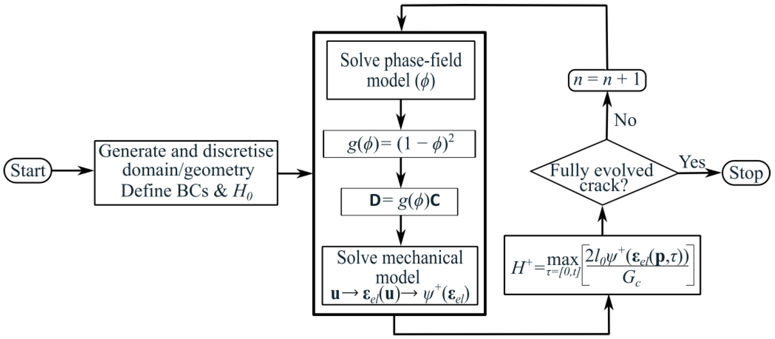
The governing equations for mechanical (1) and PF (2) models are solved in a staggered manner, as shown in Figure 1, with the following boundary conditions.

$$\mathbf{u}=\overline{\mathbf{u}} \mathrm{on} {\mathrm{\Gamma }}_{\mathrm{u}},$$

(5)

$$g\left(\varphi \right)\mathsf{\sigma }\cdot \mathbf{n}=\mathbf{t} \mathrm{on} {\mathrm{\Gamma }}_{\mathrm{t}},$$

(6)

where ${\mathrm{\Gamma }}_{\mathrm{u}} \mathrm{and} {\mathrm{\Gamma }}_{\mathrm{t}}$ are the Dirichlet and traction boundary conditions, respectively. The prescribed traction vector is denoted by $\mathbf{t}$ and $\mathbf{n}$ shows the unit normal vector.

The pre-existing crack in a geometry can be initiated in three different ways: it can be initiated by inserting a geometric discontinuity [48] by putting double nodes in the element mesh. The second way is to apply an initial condition for the PF parameter by putting $\varphi =1$ over the nodes where the initial crack exists [38,48] and $\varphi =0$ elsewhere. This study uses the third way to introduce the pre-existing cracks, which is with the help of the initial history field [19]. The history field is used because it introduces a smooth pre-existing crack that aligns naturally with the diffusive crack representation of the PFM. The history field-based crack is generated by defining a function for the shortest distance $d\left(\mathbf{p},l\right)$ from the nodes over the crack length $l$ to any position vector $\mathbf{p}$ in the domain as

$$H_0\left(\mathbf{p}\right)=B\left\{\begin{array}{l}{\displaystyle \frac{G_c}{2l_0}}\left(1-{\displaystyle \frac{2d\left(\mathbf{p},l\right)}{l_0}}\right)\hspace{1em} d\left(\mathbf{p},l\right)\le {\displaystyle \frac{l_0}{2}}\\ 0\hspace{1em}\hspace{1em}\hspace{1em}\hspace{1em}\hspace{1em}\hspace{1em}\hspace{1em}\hspace{1em}d\left(\mathbf{p},l\right)>{\displaystyle \frac{l_0}{2}}\end{array}\right., where B={\displaystyle \frac{1}{1-{\varphi }_c}}.$$

(7)

The scalar $B=1\times {10}^3$ is used, which is obtained by selecting ${\varphi }_c=1\times {10}^{-3}$ in all the simulations of this study.

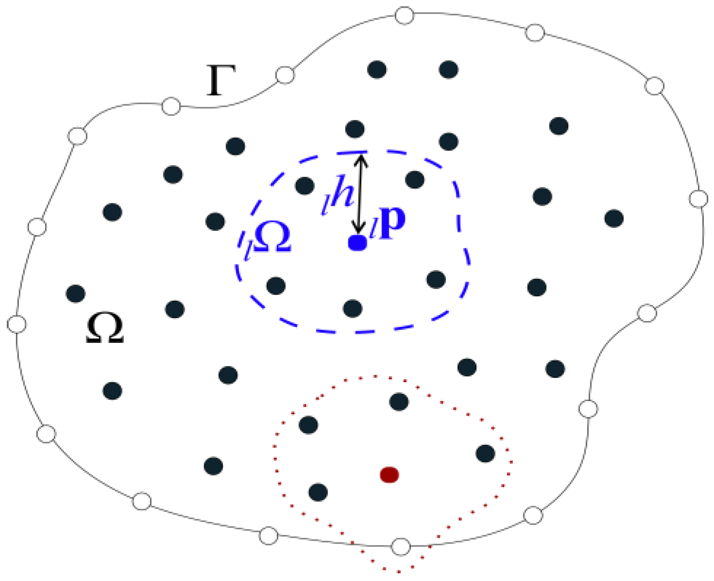
The governing equations of the PF and mechanical models are discretized using the LRBFCM [49], as shown schematically in Figure 2 with scattered node (SCN) arrangements and two local sub-domains ${}_l\mathrm{\Omega }$. The working principle of the LRBFCM is based on approximating an arbitrary function ${}_{l}f\left(\mathbf{p}\right)$ with augmented monomials $p_i\left(\mathbf{p}\right)$ in each sub-domain as

$${}_{l}f\left(\mathbf{p}\right)\approx {\displaystyle \sum _{i=1}^{{}_{l}N}{{}_l\alpha }_i{{}_l\mathrm{\Phi }}_i\left(\mathbf{p}\right)}+{\displaystyle \sum _{i=1}^M{{}_l\alpha }_{\left({}_{l}N+i\right)}{p}_i\left(\mathbf{p}\right)},$$

(8)

where ${}_{l}N$ is the number of nodes in the local sub-domain, ${}_l\alpha$ are the unknown coefficients, ${{}_l\mathrm{\Phi }}_i\left(\mathbf{p}\right)$ denotes the radial basis function (RBF), and the central node is denoted by ${}_l\mathbf{p}$. $M$ represents the number of augmented polynomials and $p_i$ denotes the respective polynomials, that is, $1,x,y,x^2,xy,\dots$. The arbitrary function ${}_{l}f\left(\mathbf{p}\right)$ in Equation (8) can be further written as

$${}_{l}f\left(\mathbf{p}\right)\approx {\displaystyle \sum _{i=1}^{{}_{l}N+M}{{}_l\alpha }_i{{}_l\mathrm{\Psi }}_i\left(\mathbf{p}\right)},$$

(9)

where ${{}_l\mathrm{\Psi }}_i\left(\mathbf{p}\right)$ is the combination of RBFs and augmented monomials, and the terms in Equation (9) can be written in a linear system of equations as

$${\displaystyle \sum _{i=1}^{{}_{l}N+M}{{}_l\mathit{A}}_{ji}{{}_l\alpha }_i}={{}_l\gamma }_j,$$

(10)

The ${{}_l\mathit{A}}_{ji}$ is the local interpolation matrix, which consists of the augmented monomials and RBFs as

$${{}_l\mathit{A}}_{ji}=\left\{\begin{array}{l}{{}_l\mathrm{\Psi }}_i\left({{}_l\mathbf{p}}_i\right)\hspace{1em} \mathrm{if} {{}_l\mathbf{p}}_i\in \mathrm{\Omega }\cup \mathrm{\Gamma } \\ p_{j-{}_{l}N}\left({{}_l\mathbf{p}}_i\right)\hspace{1em}\mathrm{if} j>{}_{l}N \mathrm{and} i\le {}_{l}N\\ 0 \hspace{1em}\hspace{1em}\hspace{1em}\hspace{1em}\mathrm{otherwise}\end{array}\right..$$

(11)

${{}_l\gamma }_j$ is the vector comprising the known values and is defined as

$${{}_l\gamma }_j=\left\{\begin{array}{l}{}_{l}f\left({{}_l\mathbf{p}}_j\right) \mathrm{if}{{}_l\mathbf{p}}_j\in \mathrm{\Omega }\cup \mathrm{\Gamma }\\ 0 \hspace{1em}\hspace{1em}\hspace{1em}\mathrm{otherwise}\end{array}\right..$$

(12)

The ${}_l\alpha$ can be calculated by inverting Equation (10) as

$${}_l\alpha ={{}_l\gamma }_j{\displaystyle \sum _{i=1}^{{}_{l}N+M}{{}_l\mathit{A}}_{ji}^{-1}}.$$

(13)

Any linear differential operator $ℒ$ can be applied to Equation (9) as

$$ℒ{}_{l}f\left(\mathbf{p}\right)\approx {\displaystyle \sum _{i=1}^{{}_{l}N+M}{{}_l\alpha }_iℒ{{}_l\mathrm{\Psi }}_i\left(\mathbf{p}\right)},$$

(14)

by putting the values of the unknown coefficients from Equations (13) to (14) can reach to

$$ℒ{}_{l}f\left(\mathbf{p}\right)\approx {\displaystyle \sum _{k=1}^{{}_{l}N+M}{{}_l\gamma }_k{\displaystyle \sum _{i=1}^{{}_{l}N+M}{{}_l\mathit{A}}_{ik}^{-1}}ℒ{{}_l\mathrm{\Psi }}_i\left(\mathbf{p}\right)}.$$

(15)

The operator weights in Equation (15), in a compact form, can be written as ${{}_l\omega }_k={\displaystyle \sum _{i=1}^{{}_{l}N+M}{{}_l\mathit{A}}_{ik}^{-1}}ℒ{{}_l\mathrm{\Psi }}_i\left(\mathbf{p}\right)$ and thus the final equation becomes

$$ℒ{}_{l}f\left(\mathbf{p}\right)\approx {\displaystyle \sum _{k=1}^{{}_{l}N+M}{{}_l\gamma }_k{{}_l\omega }_k}.$$

(16)

The solution process is illustrated schematically in Figure 1, starting with the creation and discretization of the domain and geometry. In the presence of a pre-existing crack, the history field is initialized with the help of Equation (7). After the history field is initialized, the PF and mechanical models are solved sequentially. This involves solving the PF model for the PF parameter $\varphi$, followed by the calculation of the degradation function $g\left(\varphi \right)$. Subsequently, the material properties are degraded using $g\left(\varphi \right)$, and together with the degraded properties, the mechanical model is solved for displacements. Displacements are then utilized to compute the strain tensor, and the tensile SED is determined using Equation (3), which is then compared with the history field. The history field is updated for nodes with higher SED values than the initial history field, and an additional loading increment is applied. This process continues until the material fails completely.

The PF model is solved by splitting the fourth-order differential Equation (2) of the PF into two second-order equations by assuming an auxiliary variable $\chi$ as

$${\displaystyle \frac{l_0^2}{2}}\Delta \varphi -\chi =0.$$

(17)

$$\left(H^{+}+1\right)\varphi -\chi +{\displaystyle \frac{l_0^2}{8}}\Delta \chi =H^{+}$$

(18)

The two Equations (17) and (18) are solved in a monolithic manner for the unknown PF parameter $\varphi$ using the differential operators obtained with the augmented PHSs in the meshless LRBFCM.

The mechanical model presented in Equation (1) is solved using the plane strain condition with the composed approach by directly applying the divergence operator to the stress tensor $\mathsf{\sigma }=\mathbf{D}{\nabla }^s$, explained in [35], as

$$\nabla \cdot \left[\mathbf{D}{\nabla }^s\right]\mathbf{u}=-\mathbf{b},$$

(19)

where $\mathbf{D}=g\left(\varphi \right)\mathbf{C}$ is the tensor of elasticity with degraded material properties. The symmetric gradient is denoted by ${\nabla }^s$.

The incremental loading step sizes are adjusted adaptively using the technique introduced in [36], by calculating the relative error of the current PF $\varphi$ with the initial PF ${\varphi }_{in}$ using

$$\delta \varphi =\sqrt{{\displaystyle \frac{{\displaystyle \sum _{i=1}^N{‖{\varphi }_i-{\varphi }_{in,i}‖}^2}}{{\displaystyle \sum _{i=1}^N{‖{\varphi }_{in,i}‖}^2}}}},$$

(20)

and the incremental load step size is then adjusted according to the change in PF $\delta \varphi$ as

$$\Delta u_{var}=\left\{\begin{array}{l}\Delta u_{\mathrm{large}} if \delta \varphi <0.25\\ \Delta u_{\mathrm{small}} \mathrm{otherwise}\end{array}\right..$$

(21)

In all the simulations of this study, the step size ($\Delta u_{var}$) is adjusted adaptively using Equation (20).

This approach is implemented numerically in Julia (version 1.8.0). A custom Fortran library generates matrix coefficients, which are crucial for accurate calculations. All simulations are run on an AMD Ryzen 9 7950X 16-core processor at 4.50 GHz.

3. Results

This study performs two benchmark tests, employing adaptive loading step sizes and varying node densities.

3.1. Generation of the Variable Node Density

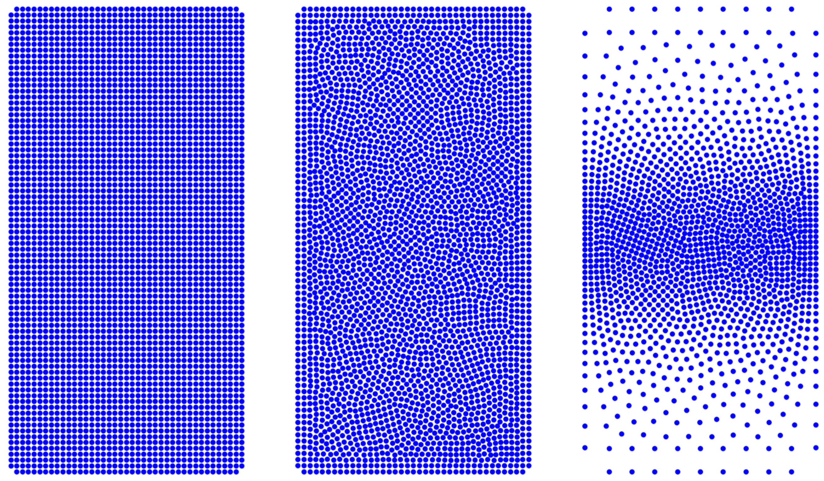
In addition to the adaptive step size, a variable node density is generated by increasing the node density around the critical regions where the crack is expected to propagate, as shown in Figure 3 and Figure 4. A node generation function $\rho \left(x,y\right)$ is employed for spatially varying node density. The node density function is composed of two parts. The first part is responsible for refining the node density in the middle region (where the initial crack is present). The second part involves refining the node density along the anticipated path of crack propagation; in the case of shear, the crack propagates from the crack’s tip towards the bottom right corner, as shown in Figure 4.

$$\rho \left(x,y\right)={\rho }_{\min }+f_{\mathrm{mid}}\left(x,y\right)+f_{\mathrm{corner}}\left(x,y\right),$$

(22)

where ${\rho }_{\min }={\displaystyle \frac{1}{h_{\max }^2}}$ is the minimum node density away from the crack in relation to the maximum node spacing $h_{\max }$, $f_{\mathrm{mid}}\left(x,y\right)$ is the function that refines the node density in the middle of the domain, and $f_{\mathrm{corner}}\left(x,y\right)$ is used for the refinement along the crack trajectory. $f_{\mathrm{mid}}\left(x,y\right)$ is a Gaussian function that controls the refinement in the middle region defined by a vertical position $d$, as

$$f_{\mathrm{mid}}\left(x,y\right)=\left\{\begin{array}{l}\left({\rho }_{\max }-{\rho }_{\min }\right){\mathrm{e}}^{\left(-{\left({\displaystyle \frac{y-d}{s}}\right)}^2\right)}, x\le x_{\mathrm{hz}}\\ 0, \hspace{1em}\hspace{1em}\hspace{1em}\hspace{1em}\hspace{1em}\hspace{1em}\hspace{1em}\hspace{1em}\hspace{1em}\mathrm{otherwise}\end{array}\right.,$$

(23)

where ${\rho }_{\max }={\displaystyle \frac{1}{h_{\min }^2}}$ is the maximum node density around the crack and the expected crack propagation path, $x_{\mathrm{hz}}$ is the horizontal point up to which the nodes are refined, and $s$ is the scaling parameter that controls the smoothness of the node distribution in the refined region. The symmetric double-notch tension (SDNT) test uses only $f_{\mathrm{mid}}\left(x,y\right)$ for the generation of node density. The $f_{\mathrm{corner}}\left(x,y\right)$, along with the $f_{\mathrm{mid}}\left(x,y\right)$, is used in the single-edge notch shear (SENS) test case. $f_{\mathrm{corner}}\left(x,y\right)$ is a refinement function that controls the refinement in the expected curved crack path as

$$f_{\mathrm{corner}}\left(x,y\right)=\left\{\begin{array}{l}\left({\rho }_{\max }-{\rho }_{\min }\right){\mathrm{e}}^{\left(-{\left({\displaystyle \frac{y-y_{\mathrm{crack}}\left(x\right)}{s+0.3\left|x-x_{\mathrm{hz}}\right|}}\right)}^2\right)}, x\ge x_{\mathrm{hz}}\\ 0, \hspace{1em} \hspace{1em}\hspace{1em}\hspace{1em}\hspace{1em}\hspace{1em}\hspace{1em}\hspace{1em}\hspace{1em}\hspace{1em}\mathrm{otherwise}\end{array}\right.,$$

(24)

where the crack path along the vertical axis is defined as

$$y_{\mathrm{crack}}\left(x\right)=x_{\mathrm{hz}}-{\displaystyle \frac{0.5\left(x-x_{\mathrm{hz}}\right)}{x_{\mathrm{end}}-x_{\mathrm{hz}}}},$$

(25)

$x_{\mathrm{end}}$ is the expected endpoint of the crack. A set of node arrangements for regular nodes (RGN), scattered nodes (SCN_uni) with uniform node spacing, and SCN_var with variable node spacings are generated using the parameters listed in

Table 1. Parameters used for the generation of the variable nodes.

Parameter	SDNT	SENS	Unit
$x_{\mathrm{hz}}$	0.5	0.51	mm
$x_{\mathrm{end}}$	-	0.81	mm
$h_{\min }$	0.0125	0.0125	mm
$h_{\max }$	0.05	0.05	mm
$d$	0.5	0.5	mm
$s$	0.25	0.25	mm
$f_{\mathrm{corner}}\left(x,y\right)$	0	$f_{\mathrm{corner}}\left(x,y\right)$	-
RGN $N$	3276	6396	-
SCNuni $N$	3200	6400	-
SCNvar $N$	1570	2310	-

for SDNT and SENS. The schemes for all node arrangements are illustrated in Figure 3 and Figure 4.

3.2. Symmetric Double-Notch Tension Test

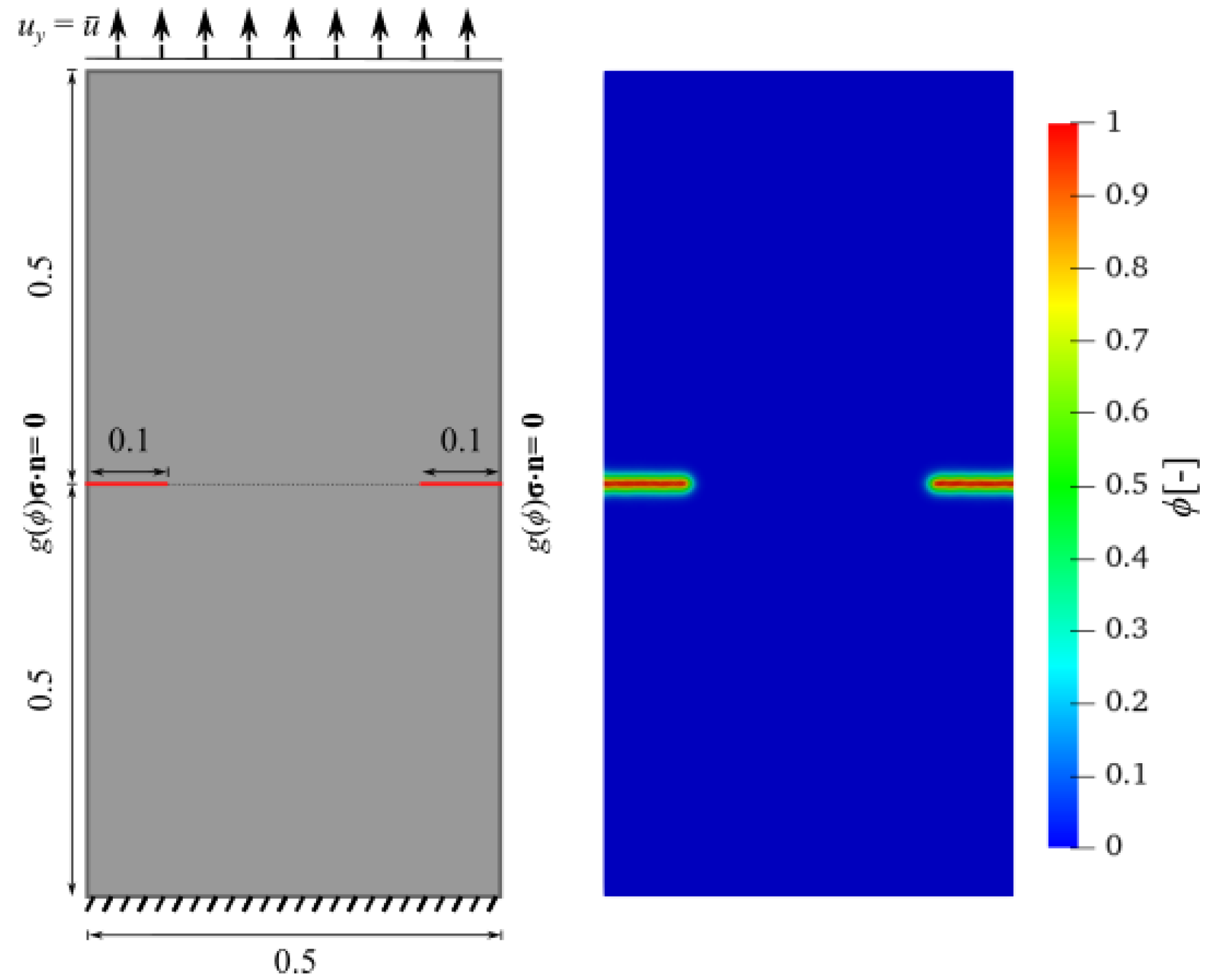
The primary purpose of selecting this test case is to demonstrate that the PFM can handle the propagation of multiple cracks. Figure 5 illustrates the geometry and boundary conditions on the left side, while the initial cracks, obtained from the initial history field, are depicted on the right. The bottom edge of the geometry is fixed, while the left and right edges are exposed to traction-free boundary conditions. The top is free to move horizontally, while an incremental load is applied vertically. The boundary stabilization technique [35,36] is employed to apply the traction boundary conditions. The boundary stabilization method shifts the boundary nodes inward by 0.5 times the minimum node spacing (h), whereas the position of the unknowns remains the same; however, the evaluation point for the boundary conditions is moved inwards. The gradient operators are then computed with these virtually shifted boundary nodes and applied to the traction-free boundary conditions.

The numerical parameters and material properties employed in the simulations are listed in

Table 2. Material properties and numerical parameters.

Parameter	Value	Unit
$E$	$210$	$\mathrm{kN}/\mathrm{m}{\mathrm{m}}^2$
$\nu$	$0.3$	-
$l_0$	$0.0075$	$\mathrm{mm}$
$G_c$	$2.7\times {10}^{-3}$	$\mathrm{kN}/\mathrm{mm}$
$h$	$0.0037$	$\mathrm{mm}$
${}_{l}N$	$13$	-
$M$	$6$	-

. The material properties are sourced from reference [50] for comparison purposes. The reference solution [50] utilizes the second-order PFM to simulate the propagation of a symmetric double-edge crack. Given the absence of a reference solution for the fourth-order PFM within this benchmark test, this study compares the results obtained from the fourth-order PFM with those derived from the second-order PFM reference solution.

The primary objective of this study is to reduce the computational time of the PFM simulation. Therefore, this study compares the results obtained with various node arrangements and loading step sizes. A constant loading step size of $\Delta u=1\times {10}^{-5} \mathrm{mm}$ and RGN with uniform arrangements. Results obtained with an adaptive loading step size using RGN, SCN_uni with uniform spacing, and SCN_var with variable node spacing are compared based on the computational time and force–displacement curves. The adaptive loading step size is based on Equation (20) with the following condition.

$$\Delta u_{var}=\left\{\begin{array}{l}1\times {10}^{-4} \mathrm{mm} \mathrm{if}\delta \varphi <0.25\\ 1\times {10}^{-5} \mathrm{mm} \mathrm{otherwise}\end{array}\right.$$

(26)

In addition to the adaptive step size, a variable node density is generated, using Equations (22)–(25), by increasing the node density around the critical regions where the crack is expected to propagate, further reducing the computational cost. $f_{\mathrm{corner}}\left(x,y\right)=0$ for the symmetric double-edge notch test. The parameters for the generated refined variable nodes in the computational domain are given in

Table 3. Parameters used for the generation of the variable nodes.

Parameter	Value	Unit
$x_{\mathrm{hz}}$	0.5	mm
$h_{\min }$	0.0037	mm
$h_{\max }$	0.02	mm
$d$	0.5	mm
$s$	$d/3$	mm
$f_{\mathrm{corner}}\left(x,y\right)$	0	-
RGN $N$	36,446	-
SCNuni $N$	36,449	-
SCNvar $N$	11,641	-

. This study defines the refined node distribution at the anticipated crack path by SCN_var.

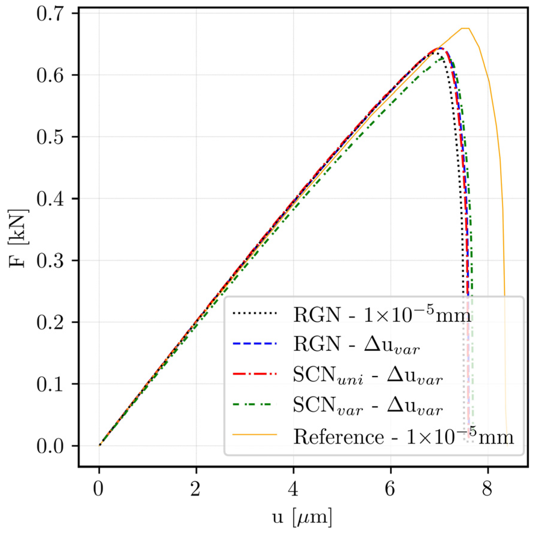
The force–displacement curves for this study, with different step size arrangements along with the reference solution, are depicted in Figure 6, where $\Delta u_{var}=1\times {10}^{-4}\to 1\times {10}^{-5} \mathrm{mm}$. All the results share an identical slope; however, the current research demonstrates earlier material failure with a marginally lower peak load. This reduced peak load is attributable to the fact that the reference solution utilizes a second-order PFM, whereas [51] reports that a fourth-order PFM generally exhibits a lower peak load than a second-order PFM. Furthermore, the reference solution employs actual notches. In contrast, this study utilizes history-based initial cracks and various node arrangements. These differences in the order of PFM, node configuration, and crack representation account for the observed variations in peak load. Nonetheless, the overall trend remains aligned with the reference solution, and the meshless LRBFCM consistently models brittle fracture with various node arrangements and loading step sizes.

Table 4. The total CPU time required using constant and adaptive loading step sizes with various node arrangements.

$\Delta \mathit{u}$ [mm]	Total Iterations	Peak-Load [kN]	CPU Time [h]
RGN $1\times {10}^{-5}$	857	0.63	4:25
RGN $\Delta u_{var}$	240	0.63	1:23
SCNuni $\Delta u_{var}$	230	0.63	1:20
SCNvar $\Delta u_{var}$	168	0.62	0:09

presents the total number of iterations, CPU time required for the simulations, and the peak load for different node configurations under both adaptive and constant loading step sizes. The improved computational efficiency from using variable node density, combined with adaptive loading step sizes, is clearly demonstrated in Table 4. This test case investigates four scenarios: RGN with constant loading increments of $\Delta u=1\times {10}^{-5} \mathrm{mm}$, RGN, SCN_uni with uniform node spacings, and SCN_var with variable node spacings using adaptive step sizes $\Delta u_{var}$.

In the RGN arrangements, 857 loading increments were performed using a constant and small step size, leading to a simulation duration of 4 h and 25 min of CPU time. The small step size helps ensure accurate results, but it also results in high computational costs because a small loading increment is used even in the linear elastic region.

Employing an adaptive loading step size strategy with the RGN arrangements, the total number of iterations was substantially decreased to 240, and the CPU time was reduced to 1 h and 23 min. This reduction in CPU time is attributable to the adaptive algorithm’s ability to automatically adjust the loading increment based on the non-linear response of the coupled system. The adaptive loading step size method reduces CPU time while maintaining accuracy, as demonstrated by the identical peak load (0.63 kN) value in both cases.

The SCN_uni arrangements, with adaptive loading step size, further enhance computational efficiency by reducing the CPU time to 1 h and 20 min. The comparable peak-load response (0.63 kN) demonstrates that the scattered node arrangement preserves solution accuracy while enhancing numerical efficiency.

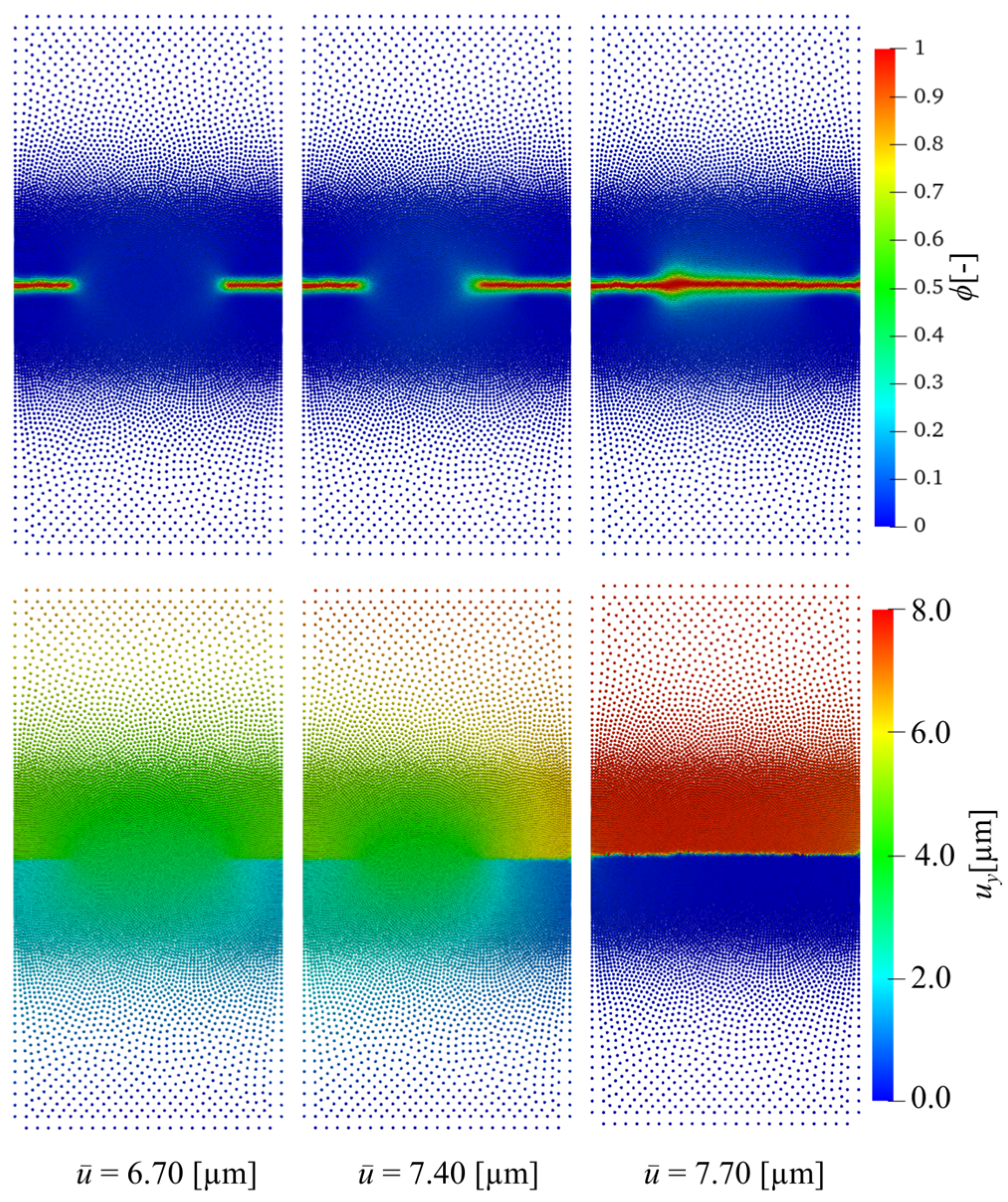
The SCN_var arrangements improved efficiency by integrating with the adaptive step size strategy. The simulation completed in 168 loading steps, requiring just 9 min of CPU time, which is approximately 30 times faster than RGN with uniform nodes and constant loading step size. It generated the same force–displacement graphs with a peak load of 0.62 kN. This significant decrease in computation time shows the effectiveness of the adaptive loading step size strategy with spatially variable node density. These results demonstrate that using SCN_var, particularly with adaptive loading, enables highly efficient simulations without compromising numerical stability or accuracy. Focusing computational resources solely on areas of interest, like around the moving crack front, can significantly reduce the overall simulation cost. The evolution of the PF and displacement fields at three different stages of the simulation, with the respective applied load, is shown in Figure 7.

3.3. Single-Edge Notch Shear Test

The single-edge notch shear (SENS) test is included to assess the robustness of the proposed framework further. The SENS subjected to shear load entails a complex loading and crack propagation scenario, facilitating the evaluation of the model’s stability, computational efficiency, and accuracy across various conditions. The objective is to verify that the efficiency improvements observed in the previous test, which resulted from integrating adaptive loading step size and variable node density, are consistently maintained across different fracture problems.

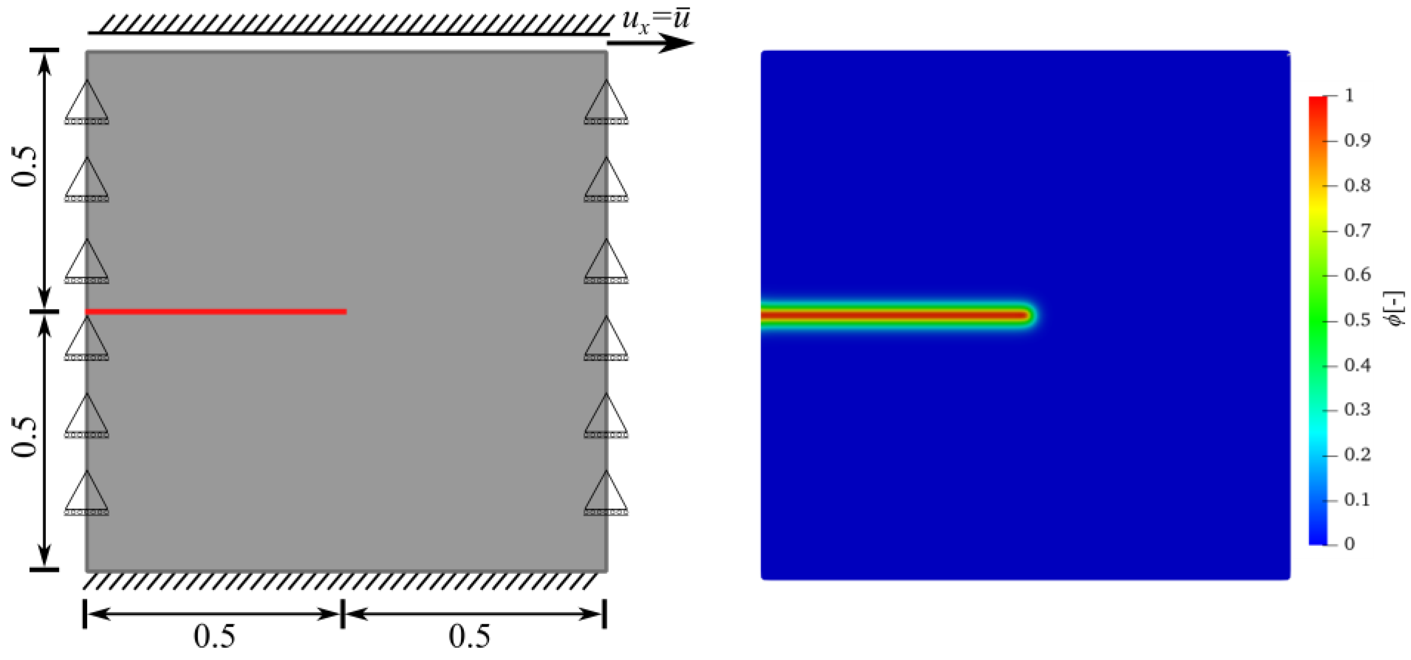
The geometry and boundary conditions are depicted in Figure 8, where the lower edge is fixed in both horizontal and vertical directions. The left and right edges are constrained in the vertical direction but are free to move horizontally. The upper edge is restricted vertically, and an incremental load is applied in the horizontal direction. The numerical parameters and material properties are listed in

Table 5. Material properties and numerical parameters.

Parameter	Value	Unit
$E$	$210$	$\mathrm{kN}/\mathrm{m}{\mathrm{m}}^2$
$\nu$	$0.3$	-
$l_0$	$0.015$	$\mathrm{mm}$
$G_c$	$2.7\times {10}^{-3}$	$\mathrm{kN}/\mathrm{mm}$
$h$	$0.00625$	$\mathrm{mm}$
${}_{l}N$	$13$	-
$M$	$6$	-

, where the material properties are taken from the reference article [52].

Similarly to the previous case, the variable node density was generated with high node density in the expected path of crack propagation. The parameters used to generate the nodes for the SENS test case are listed in

Table 6. Parameters used for generating the variable nodes.

Parameter	Value	Unit
$x_{\mathrm{hz}}$	0.51	mm
$x_{\mathrm{end}}$	0.81	mm
$h_{\min }$	0.00625	mm
$h_{\max }$	0.02	mm
$d$	0.5	mm
$s$	$d/3$	mm
RGN $N$	25,596	-
SCNuni $N$	25,600	-
SCNvar $N$	11,465	-

.

Upon defining all the parameters and using Equations (22)–(25), a variable node arrangement (SCN_var) is generated. The total number of nodes for RGN, SCN_uni, and SCN_var is given in Table 6. The node count in SCN_var is less than half that in RGN and SCN_uni, hence the computational cost will be lower.

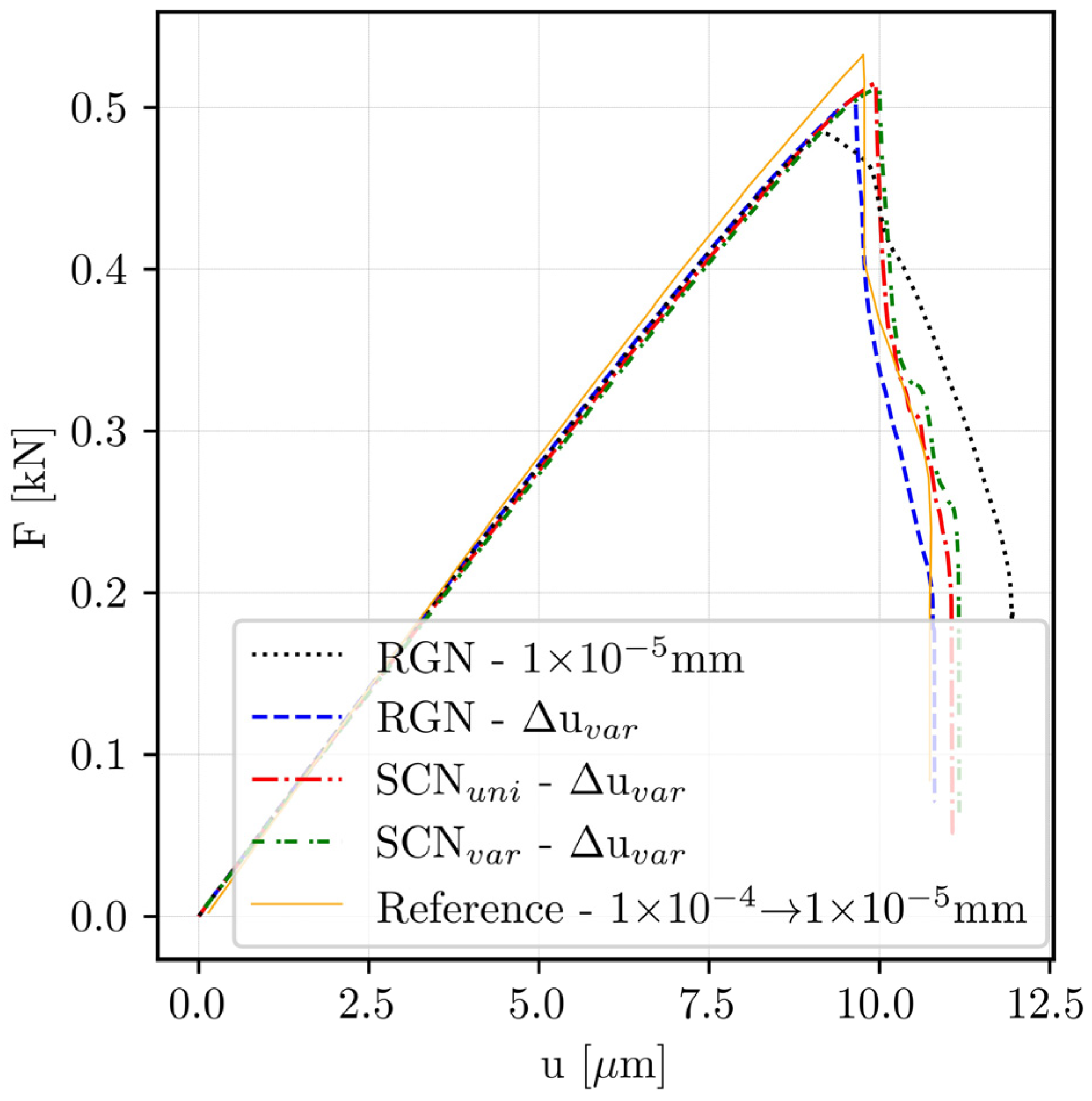
The force–displacement graphs depicted in Figure 9 and the total CPU time presented in

Table 7. The total CPU time required using constant and adaptive loading step sizes with various node arrangements.

$\Delta \mathit{u}$ [mm]	Total Iterations	Peak-Load [kN]	CPU Time [h]
RGN $1\times {10}^{-5}$	1198	0.48	3:41
RGN $\Delta u_{var}$	1193	0.50	4:09
SCNuni $\Delta u_{var}$	1202	0.51	4:22
SCNvar $\Delta u_{var}$	1288	0.51	1:15

provide a comprehensive evaluation of the efficiency and performance of the proposed methodology. The adaptive loading step size for the shear test case is defined as $\Delta u_{var}=5\times {10}^{-4}\to 1\times {10}^{-6} \mathrm{mm}$. These findings confirm that the adaptive loading scheme combined with the variable node density approach successfully maintains high accuracy while significantly reducing computational costs.

The force–displacement curves presented in Figure 9 for the RGN, SCN_uni, and SCN_var configurations align closely with the reference solution. The reference solution [52] utilized a load increment of $\Delta u=1\times {10}^{-4} \mathrm{mm}$ during the initial eighty steps, then manually increased to $\Delta u=1\times {10}^{-5} \mathrm{mm}$ for the following steps. The adaptive load step size strategy employed in this study yielded results comparable to the reference solution [52], thereby confirming the robustness and precision of the proposed framework.

The RGN, with a constant $\Delta u=1\times {10}^{-5} \mathrm{mm}$, exhibits marginally different behavior in capturing the peak load compared to the reference solution [52]. It exhibits smooth softening after reaching the peak load. This behavior is attributed to the load step size, which is not sufficiently small to accurately capture the crack behavior. In contrast, using the adaptive loading step size strategy significantly improves this behavior and precisely captures crack propagation in the RGN, SCN_uni, and SCN_var node arrangements.

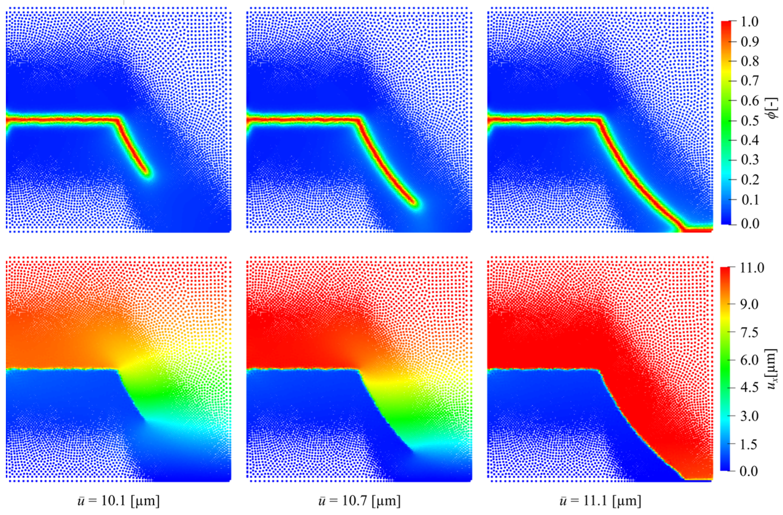
Table 7 shows the statistical analysis of computational efficiency. The constant $\Delta u=1\times {10}^{-5} \mathrm{mm}$ enables the simulations to be completed within 3 h and 41 min; however, the force–displacement curve does not closely align with the reference solution [52]. Implementing the adaptive loading step size for RGN and SCN_uni arrangements resulted in increased CPU times of 4 h and 9 min and 4 h and 22 min, respectively. The prolonged CPU duration is primarily attributable to the finer increments employed within the non-linear regime. However, the adaptive stepping ($\Delta u_{var}$) ensured results closely matched the reference solution and offered better accuracy in the post-peak region. The SCN_var arrangements completed the simulation in only 1 h and 15 min of CPU time, demonstrating highly efficient performance with approximately three times reduction in computational time relative to cases with uniform node arrangements, while still maintaining accuracy. Figure 10 illustrates the evolution of the PF and displacement fields at three distinct stages of the simulation, along with the corresponding applied load.

4. Conclusions

This study presents an adaptive step size strategy integrated with variable node density to reduce the computation cost. Two benchmark tests, the symmetric double-notch tension test and a SENS test, were used to analyze the proposed framework. Identical numerical tests were performed for both benchmarks, ensuring consistent assessment of the proposed methodology’s efficiency and accuracy.

All configurations accurately reproduced the force–displacement graphs for symmetric crack propagation in the first benchmark. Although the RGN with uniform node distributions and a constant loading increment ($\Delta u=1\times {10}^{-5} \mathrm{mm}$) produced consistent and stable results, it required significantly more time to compute due to the uniform node spacing maintained throughout the entire domain. The adaptive loading step size strategy ($\Delta u_{var}$) allows the solver to automatically decrease the time step near the peak load, where nonlinearities are more pronounced. Consequently, computational time was reduced for RGN and SCN_uni without losing accuracy.

The enhancement in computational efficiency became more pronounced when the SCN_var was utilized, while maintaining high accuracy and substantially reducing the computational time. As shown in Table 4, the SCN_var configurations reduce the total CPU time by about 30 times, in the computational environment used in this study, relative to RGN, while maintaining identical peak-load and crack propagation patterns. This enhancement is achieved by concentrating computational resources in critical regions by increasing node density along the anticipated crack propagation path, while preserving a coarser node density in other areas.

The SENS showed a similar trend; all node configurations precisely captured the crack propagation, and the force–displacement curves aligned well with the reference solution. The SCN_var arrangements reduced the total CPU time by approximately three times in comparison to RGN, as shown in Table 7. These findings demonstrate that both the SCN_var and the adaptive loading step size strategy can significantly reduce computational time in these benchmark tests without compromising accuracy. However, the extent of these computational efficiency improvements can differ based on the crack configuration, solver implementation, and hardware configuration.

The current study demonstrates that increasing node density exclusively in regions of interest offers a good balance between computational efficiency and predictive accuracy, thereby facilitating future research on the implementation of adaptive node redistribution. This advancement will support large-scale industrial fracture simulations employing strong-form meshless methods.

The proposed adaptive stepping strategy is versatile and relies solely on the evolution of the PF variable, without assuming any specific geometry or crack pattern. However, the current study does not address complex or multiple interacting cracks. The application of this method to handle complicated crack networks and geometries would require further investigation, particularly the extension to three dimensions, and thus represents a key future research direction. Therefore, these limitations should be taken into account when addressing complex fracture problems using this approach.

References

1. Griffith, A.A. The phenomena of rupture and flow in solids. Phil. Trans. R. Soc. Lond. A 1921, 221, 163–198. [Google Scholar]
2. Irwin, G.R. Analysis of stresses and strains near the end of a crack traversing a plate. J. Appl. Mech. 1957, 24, 361–364. [Google Scholar] [CrossRef]
3. Egger, A.; Pillai, U.; Agathos, K.; Kakouris, E.; Chatzi, E.; Aschroft, I.A.; Triantafyllou, S.P. Discrete and phase field methods for linear elastic fracture mechanics: A comparative study and state-of-the-art review. Appl. Sci. 2019, 9, 2436. [Google Scholar] [CrossRef]
4. Francfort, G.A.; Marigo, J.-J. Revisiting brittle fracture as an energy minimization problem. J. Mech. Phys. Solids 1998, 46, 1319–1342. [Google Scholar] [CrossRef]
5. Bourdin, B.; Francfort, G.A.; Marigo, J.-J. Numerical experiments in revisited brittle fracture. J. Mech. Phys. Solids 2000, 48, 797–826. [Google Scholar] [CrossRef]
6. Karma, A.; Kessler, D.A.; Levine, H. Phase-Field Model of Mode III Dynamic Fracture. Phys. Rev. Lett. 2001, 87, 045501. [Google Scholar] [CrossRef]
7. Martínez-Pañeda, E.; Golahmar, A.; Niordson, C.F. A phase field formulation for hydrogen assisted cracking. Comput. Methods Appl. Mech. Eng. 2018, 342, 742–761. [Google Scholar] [CrossRef]
8. Ali, I.; Vuga, G.; Mavrič, B.; Šarler, B. A fourth-order phase-field model of crack initiation and propagation under thermomechanical loading solved with strong-form meshless method. Theor. Appl. Fract. Mech. 2025, 139, 105078. [Google Scholar] [CrossRef]
9. Bourdin, B. Numerical implementation of the variational formulation for quasi-static brittle fracture. Interfaces Free Bound. 2007, 9, 411–430. [Google Scholar] [CrossRef]
10. Miehe, C.; Hofacker, M.; Welschinger, F. A phase field model for rate-independent crack propagation: Robust algorithmic implementation based on operator splits. Comput. Methods Appl. Mech. Eng. 2010, 199, 2765–2778. [Google Scholar] [CrossRef]
11. Miehe, C.; Welschinger, F.; Hofacker, M. Thermodynamically consistent phase-field models of fracture: Variational principles and multi-field FE implementations. Int. J. Numer. Meth. Eng. 2010, 83, 1273–1311. [Google Scholar] [CrossRef]
12. Ambati, M.; Gerasimov, T.; De Lorenzis, L. A review on phase-field models of brittle fracture and a new fast hybrid formulation. Comput. Mech. 2015, 55, 383–405. [Google Scholar] [CrossRef]
13. Ambati, M.; Kruse, R.; De Lorenzis, L. A phase-field model for ductile fracture at finite strains and its experimental verification. Comput Mech 2016, 57, 149–167. [Google Scholar] [CrossRef]
14. Aurojyoti, P.; Rajagopal, A. Fourth order phase field modeling of brittle fracture by Natural element method. Int. J. Fract. 2024, 247, 203–224. [Google Scholar] [CrossRef]
15. Borden, M.J.; Hughes, T.J.R.; Landis, C.M.; Anvari, A.; Lee, I.J. A phase-field formulation for fracture in ductile materials: Finite deformation balance law derivation, plastic degradation, and stress triaxiality effects. Comput. Methods Appl. Mech. Eng. 2016, 312, 130–166. [Google Scholar] [CrossRef]
16. Prakash, V.; Behera, A.K.; Rahaman, M.M. A phase-field model for thermo-mechanical fracture. Math. Mech. Solids 2023, 28, 533–561. [Google Scholar] [CrossRef]
17. Dong, X.; Hirshikesh, H.; Yu, T.; Zhang, Q.; Natarajan, S. A framework to model freeze/thaw-induced crack propagation in concrete based on a fatigue phase-field method. Eng. Fract. Mech. 2024, 306, 110260. [Google Scholar] [CrossRef]
18. Golahmar, A.; Kristensen, P.K.; Niordson, C.F.; Martínez-Pañeda, E. A phase field model for hydrogen-assisted fatigue. Int. J. Fatigue 2022, 154, 106521. [Google Scholar] [CrossRef]
19. Borden, M.J.; Verhoosel, C.V.; Scott, M.A.; Hughes, T.J.R.; Landis, C.M. A phase-field description of dynamic brittle fracture. Comput. Methods Appl. Mech. Eng. 2012, 217–220, 77–95. [Google Scholar] [CrossRef]
20. Li, H.; Wang, W.; Cao, Y.; Liu, S. Phase-Field Modeling Fracture in Anisotropic Materials ed F Huang. Adv. Civ. Eng. 2021, 2021, 4313755. [Google Scholar] [CrossRef]
21. Gmati, H.; Mareau, C.; Ammar, A.; El Arem, S. A phase-field model for brittle fracture of anisotropic materials. Int. J. Numer. Methods Eng. 2020, 121, 3362–3381. [Google Scholar] [CrossRef]
22. Kakouris, E.G.; Triantafyllou, S.P. Material point method for crack propagation in anisotropic media: A phase field approach. Arch. Appl. Mech. 2018, 88, 287–316. [Google Scholar] [CrossRef]
23. Wu, J.-Y. A unified phase-field theory for the mechanics of damage and quasi-brittle failure. J. Mech. Phys. Solids 2017, 103, 72–99. [Google Scholar] [CrossRef]
24. Ali, I.; Vuga, G.; Mavrič, B.; Hanoglu, U.; Šarler, B. Fourth-order phase field modelling of brittle fracture with strong form meshless method. Eng. Anal. Bound. Elem. 2024, 169, 106025. [Google Scholar] [CrossRef]
25. Marandi, S.M.; Nourbakhsh, S.H.; Botshekanan Dehkordi, M.; Badnava, H. Finite element implementation of coupled temperature-rate dependent fracture using the phase field model. Mech. Mater. 2020, 148, 103449. [Google Scholar] [CrossRef]
26. Ambati, M.; Gerasimov, T.; De Lorenzis, L. Phase-field modeling of ductile fracture. Comput. Mech. 2015, 55, 1017–1040. [Google Scholar] [CrossRef]
27. Rabczuk, T.; Belytschko, T. Cracking particles: A simplified meshfree method for arbitrary evolving cracks. Numer. Meth Eng. 2004, 61, 2316–2343. [Google Scholar] [CrossRef]
28. Nguyen, V.P.; Rabczuk, T.; Bordas, S.; Duflot, M. Meshless methods: A review and computer implementation aspects. Math. Comput. Simul. 2008, 79, 763–813. [Google Scholar] [CrossRef]
29. Yang, Y.; Cheng, Y.; Peng, M.; Cheng, H. The complex variable element-free Galerkin method based on the conjugate basis function for 3D elastoplastic problems. Eng. Anal. Bound. Elem. 2025, 179, 106425. [Google Scholar] [CrossRef]
30. Cheng, Y.; Li, J. A complex variable meshless method for fracture problems. Sci. China Ser. G 2006, 49, 46–59. [Google Scholar] [CrossRef]
31. Dobravec, T.; Mavrič, B.; Zahoor, R.; Šarler, B. A coupled domain–boundary type meshless method for phase-field modelling of dendritic solidification with the fluid flow. Int. J. Numer. Methods Heat Fluid Flow 2023, 33, 2963–2981. [Google Scholar] [CrossRef]
32. Šarler, B.; Vertnik, R. Meshfree explicit local radial basis function collocation method for diffusion problems. Comput. Math. Appl. 2006, 51, 1269–1282. [Google Scholar] [CrossRef]
33. Fasshauer, G.E. Meshfree Approximation Methods with Matlab: (With CD-ROM); World Scientific: Singapore, 2007; Volume 6. [Google Scholar]
34. Mavrič, B.; Sarler, B. Local radial basis function collocation method for linear thermoelasticity in two dimensions. Int. J. Numer. Methods Heat Fluid Flow 2015, 25, 1488–1510. [Google Scholar] [CrossRef]
35. Vuga, G.; Mavrič, B.; Šarler, B. An improved local radial basis function method for solving small-strain elasto-plasticity. Comput. Methods Appl. Mech. Eng. 2024, 418, 116501. [Google Scholar] [CrossRef]
36. Ali, I.; Vuga, G.; Mavrič, B.; Šarler, B. Meshless solution of the crack propagation in brittle elastic material under shear, compressible and tensile loading. Eng. Fract. Mech. 2025, 323, 111207. [Google Scholar] [CrossRef]
37. Goswami, S.; Anitescu, C.; Rabczuk, T. Adaptive fourth-order phase field analysis for brittle fracture. Comput. Methods Appl. Mech. Eng. 2020, 361, 112808. [Google Scholar] [CrossRef]
38. Hirshikesh Pramod, A.L.N.; Annabattula, R.K.; Ooi, E.T.; Song, C.; Natarajan, S. Adaptive phase-field modeling of brittle fracture using the scaled boundary finite element method. Comput. Methods Appl. Mech. Eng. 2019, 355, 284–307. [Google Scholar] [CrossRef]
39. Yu, Y.; Hou, C.; Zheng, X.; Rabczuk, T.; Zhao, M. An efficient and robust staggered scheme based on adaptive time field for phase field fracture model. Eng. Fract. Mech. 2024, 301, 110025. [Google Scholar] [CrossRef]
40. Heister, T.; Wheeler, M.F.; Wick, T. A primal-dual active set method and predictor-corrector mesh adaptivity for computing fracture propagation using a phase-field approach. Comput. Methods Appl. Mech. Eng. 2015, 290, 466–495. [Google Scholar] [CrossRef]
41. Hirshikesh Natarajan, S.; Annabattula, R.K. A FEniCS implementation of the phase field method for quasi-static brittle fracture. Front. Struct. Civ. Eng. 2019, 13, 380–396. [Google Scholar] [CrossRef]
42. Hirshikesh Schneider, D.; Nestler, B. Realization of adaptive mesh refinement for phase-field model of thermal fracture within the FEniCS framework. Eng. Fract. Mech. 2023, 293, 109676. [Google Scholar] [CrossRef]
43. Li, W.; Ambati, M.; Nguyen-Thanh, N.; Du, H.; Zhou, K. Adaptive fourth-order phase-field modeling of ductile fracture using an isogeometric-meshfree approach. Comput. Methods Appl. Mech. Eng. 2023, 406, 115861. [Google Scholar] [CrossRef]
44. Li, P.; Qiu, W.; Wu, J.; Wu, Y.; Hu, K.; Zhao, L. Fourth-order phase field modeling of dynamic fracture in porous brittle materials using an adaptive isogeometric analysis. Eng. Fract. Mech. 2025, 315, 110763. [Google Scholar] [CrossRef]
45. Si, Z.; Hirshikesh Yu, T.; Fang, W.; Natarajan, S. Mixed-mode thermo-mechanical fracture: An adaptive multi-patch isogeometric phase-field cohesive zone model. Comput. Methods Appl. Mech. Eng. 2024, 431, 117330. [Google Scholar] [CrossRef]
46. Tanné, E.; Li, T.; Bourdin, B.; Marigo, J.-J.; Maurini, C. Crack nucleation in variational phase-field models of brittle fracture. J. Mech. Phys. Solids 2018, 110, 80–99. [Google Scholar] [CrossRef]
47. Li, G.; Zhang, M.; Zhou, J. A phase field model with modified volumetric-deviatoric decomposition for the mixed-mode fracture of rock. Comput. Geotech. 2024, 176, 106738. [Google Scholar] [CrossRef]
48. Zhuang, X.; Zhou, S.; Huynh, G.D.; Areias, P.; Rabczuk, T. Phase field modeling and computer implementation: A review. Eng. Fract. Mech. 2022, 262, 108234. [Google Scholar] [CrossRef]
49. Vertnik, R.; Šarler, B. Meshless local radial basis function collocation method for convective-diffusive solid-liquid phase change problems. Int. J. Numer. Methods Heat Fluid Flow 2006, 16, 617–640. [Google Scholar] [CrossRef]
50. Molnár, G.; Gravouil, A. 2D and 3D Abaqus implementation of a robust staggered phase-field solution for modeling brittle fracture. Finite Elem. Anal. Des. 2017, 130, 27–38. [Google Scholar] [CrossRef]
51. Li, Y.; Yu, T.; Xing, C.; Natarajan, S. Crack growth in homogeneous media using an adaptive isogeometric fourth-order phase-field model. Comput. Methods Appl. Mech. Eng. 2023, 413, 116122. [Google Scholar] [CrossRef]
52. Yu, Y.; Hou, C.; Zheng, X.; Rabczuk, T.; Zhao, M. A generally variational phase field model of fracture. Theor. Appl. Fract. Mech. 2023, 128, 104111. [Google Scholar] [CrossRef]
Figure 1. Solution procedure.
Mathematics 13 03795 g001
Figure 2. Domain Ω and boundary Γ representations are illustrated using SCN arrangements. Interior nodes are depicted as solid circles, whereas hollow circles represent boundary nodes. Two sub-domains Ω l are indicated with dotted and dashed lines. The variable h l denotes the mean distance from the central point p l to the neighboring nodes within each sub-domain.
Mathematics 13 03795 g002
Figure 3. Different node arrangements for the SDNT test with total nodes in the domain and a refined node density in the expected crack propagation path.
Mathematics 13 03795 g003
Figure 4. Different node arrangements for the SENS test with total nodes in the domain and a refined node density in the expected crack propagation path.
Mathematics 13 03795 g004
Figure 5. Geometry and boundary conditions (left), pre-existing cracks (right). All measurements are in millimeters.
Mathematics 13 03795 g005
Figure 6. Force–displacement graphs with various node arrangements and loading step sizes.
Mathematics 13 03795 g006
Figure 7. PF (top) and displacement (bottom) fields evolution at different applied loads.
Mathematics 13 03795 g007
Figure 8. Geometry and boundary conditions with an initial crack as red line (left), pre-existing crack (right). All measurements are in millimeters.
Mathematics 13 03795 g008
Figure 9. Force–displacement graphs with various node arrangements and loading step sizes. In the reference solution, 1 × 10 4 1 × 10 5   mm means that the initial eighty steps use Δ u = 1 × 10 4   mm , and then Δ u = 1 × 10 5   mm .
Mathematics 13 03795 g009
Figure 10. PF (top) and displacement (bottom) fields evolution at different applied loads.
Mathematics 13 03795 g010