Abstract
This paper investigates an infinite-horizon optimal consumption and investment problem for an agent who consumes two types of goods: necessities and luxuries. The agent derives utility from both goods but faces a ratcheting constraint on luxury consumption, which prohibits any decline in its level over time. This constraint captures the irreversible nature of high living standards or luxury habits often observed in real economies. We formulate the problem in a complete financial market with a risk-free asset and a risky stock and solve it analytically using the dual–martingale method. The dual problem is shown to reduce to a family of optimal stopping problems, from which we derive explicit closed-form solutions for the value function and optimal policies. Our results reveal that the ratcheting constraint generates asymmetric consumption dynamics: necessities adjust freely, whereas luxuries exhibit downward rigidity. As a consequence, the marginal propensity to consume necessities declines with wealth, while luxury consumption and portfolio risk exposure increase more sharply compared to the benchmark case without ratcheting. The model provides a continuous-time microfoundation for persistent high consumption levels and greater risk-taking among wealthy individuals.
Keywords:
consumption ratcheting; luxury goods; duality; optimal stopping; portfolio choice; marginal propensity to consume; risk-taking MSC:
91B42; 91G10; 91G80; 93E20; 60H30; 35R35
1. Introduction
Understanding how individuals adjust their consumption and investment behavior when faced with changing wealth and lifestyle standards is a central question in financial economics. While the classical greenstudies of Merton [1,2] provide the foundation for continuous-time consumption and portfolio choice, these models assume that consumption is fully flexible and can both rise and fall smoothly over time. However, empirical evidence suggests that many households exhibit strong resistance to lowering their standard of living once it has been raised, particularly with respect to luxury consumption. This phenomenon—often referred to as the ratcheting effect—implies that the consumption of certain goods may be irreversible or downward-rigid.
The idea of consumption ratcheting goes back to the classic work of Duesenberry [3], and was first formalized in a continuous-time framework by Dybvig [4], who modeled an agent with intolerance for any decline in the overall standard of living. Subsequent research, including Campbell and Cochrane [5] and Carroll [6], emphasized the behavioral and macroeconomic implications of habit persistence and relative consumption concerns. In parallel, empirical studies such as Aït-Sahalia et al. [7] and Wachter and Yogo [8] highlighted that luxury goods exhibit high income elasticity and are disproportionately consumed by wealthy households, suggesting that maintaining luxury consumption is an important determinant of portfolio behavior and wealth accumulation.
In this paper, we focus on consumption ratcheting in luxury goods. Unlike Dybvig’s model, where the entire consumption level is subject to ratcheting, we distinguish between two categories of goods—necessities and luxuries—and impose the ratcheting constraint only on the latter. This specification captures the stylized fact that individuals can easily reduce spending on necessities but are reluctant to reduce luxury consumption once a certain social or lifestyle benchmark is reached. Economically, such a constraint can be interpreted as reflecting reputational concerns, habit persistence in luxury preferences, or psychological loss aversion associated with downward adjustments in status consumption.
Relative to the seminal ratcheting model of Dybvig [4], where the entire consumption stream is subject to a non-decreasing constraint, our framework differs in two key respects. First, we distinguish between a flexible “necessity” component and a ratcheted “luxury” component, which allows us to capture Engel-type patterns in a tractable continuous-time setting. Second, we show that, even in this two-good environment, the dual problem reduces to an optimal stopping problem that admits closed-form policy functions and sharp comparative statics. To the best of our knowledge, such an explicit analytical characterization with luxury-specific ratcheting has not been derived in the existing continuous-time literature on habit formation or consumption ratcheting.
Typical examples include private-school tuition, club memberships, luxury automobiles, and high-end housing. Once a household has committed to such items, scaling them down is often perceived as a social or psychological loss, and households instead adjust more flexible categories (such as generic consumption or savings). Qualitative evidence in household finance and marketing suggests that even during downturns, affluent households tend to preserve these “visible” luxury expenditures while cutting back on necessities or precautionary savings, which is precisely the kind of behavior our luxury-specific ratcheting constraint is intended to capture.
We formulate the problem in an infinite-horizon continuous-time economy with a risk-free asset and a risky stock, where the agent allocates wealth optimally across consumption of both goods and portfolio investment. By employing the dual-martingale method of Cox and Huang [9] and following the approach of Peskir [10], we show that the dual problem can be reduced to a family of optimal stopping problems. This structure allows us to derive explicit closed-form solutions for the value function, optimal consumption policies, and portfolio allocations under the ratcheting constraint.
The rest of the paper is organized as follows. Section 2 introduces the model setup and preference specification with ratcheting in luxury goods. Section 3 analyzes the benchmark model without ratcheting and then derives the optimal strategies for the ratcheting model using the dual–martingale approach. We also investigate the asymptotic behavior of the optimal solutions and provide their economic interpretations. Section 4 concludes.
2. The Economy
We consider a consumption and portfolio selection problem of an infinitely lived agent with two consumption goods: a necessity good and a luxury good, denoted by and , respectively. Following the theory in Dybvig [4], we assume that the agent experiences strong aversion to any decline in the consumption of luxury goods. Hence, her/his consumption process for luxury goods, , must satisfy the ratcheting constraint , where represents the consumption level just prior to time t. In other words, must be a non-decreasing, right-continuous process. This constraint captures the notion of “habit persistence in luxury consumption,” meaning that once the agent’s standard of luxury rises, it cannot be lowered without incurring psychological discomfort or social loss. We assume that the initial luxury consumption level is given.
The agent’s intertemporal preference is represented by the expected utility function
where is the subjective discount factor, is the weight placed on utility derived from the luxury good, and is a shift parameter capturing a baseline level of luxury services (for instance, access to a minimum status good or a stock of durable luxury items). The term L ensures that the marginal utility from the luxury good remains finite even when and helps generate interior solutions in the optimal consumption problem.
The inequality implies that the utility from necessity consumption is more curved than that from luxury consumption, so the agent behaves as more risk-averse with respect to necessities than luxuries. The shift parameter L makes the felicity from luxury goods of a modified Stone–Geary form, which belongs to the HARA family [2], and ensures that marginal utility from luxury goods remains finite at . This specification captures the idea that necessities are essential, whereas luxury goods provide additional satisfaction above a baseline level and can be postponed when resources are scarce.
The elasticity of marginal utility of a utility function is defined as . For the necessity good, this elasticity is constant and equal to , while for the luxury good it is , which increases with . This implies that as the level of luxury consumption rises, the agent becomes relatively more risk-averse with respect to that good, reflecting satiation effects and diminishing marginal pleasure from luxury consumption. Moreover, the luxury good exhibits an income elasticity greater than one for sufficiently high income levels in a static optimization problem, consistent with Engel’s law and the empirical classification of luxury goods.
Blinder [11] considers a similar utility specification for consumption and bequest with , while Carroll [6] adopts the same specification as Equation (1) for consumption and wealth. The felicity function for the luxury good takes a modified Stone–Geary form and thus belongs to the class of hyperbolic absolute risk aversion (HARA) utility functions [2]. Note that the marginal utility of the necessity good is infinite when , whereas when , the marginal utility of the luxury good remains finite even if . This ensures interiority of the solution and guarantees that the agent will always consume a positive amount of necessity goods before allocating wealth to luxury goods.
- Financial Market. The financial market consists of a risk-free asset and a risky asset. The risk-free asset yields a constant rate of return . The price process of the risky asset evolves according towhere denotes the expected continuously compounded rate of return on the risky asset, and is its volatility. The parameter is the market price of risk (Sharpe ratio) associated with holding the risky asset, and is a standard Brownian motion defined on a complete probability space endowed with the augmented filtration generated by (see Karatzas and Shreve [12] for details on the mathematical and probabilistic foundations). This market structure corresponds to the classical complete market setting of Merton [2], allowing the agent to continuously trade to smooth marginal utilities across goods and over time, subject to the ratcheting constraint on luxury consumption.
- Wealth Dynamics. The agent’s wealth process evolves according towhere denotes the dollar amount invested in the risky asset at time t, and and represent the consumption rates of necessity and luxury goods, respectively. These processes satisfy the standard integrability conditions: for all ,We denote by the initial wealth, and impose the transversality condition .Following Cox and Huang [9], we can rewrite the dynamic budget constraint Equation (3) in its static (martingale) form aswhereHere, is the stochastic discount factor (or state-price density), and is the market price of risk. The static form Equation (4) highlights that optimal consumption and investment choices can be interpreted as intertemporal allocations of wealth across states and goods, discounted by state prices. This representation will be particularly useful for applying duality methods in the subsequent analysis.
3. Optimization Problem
3.1. Benchmark Model
The agent’s optimization problem can be stated as follows:
Problem 1.
We make the following assumption which guarantees that a solution to Problem 1 exists.
Assumption 1.
We assume that
Economically, can be interpreted as a risk-adjusted effective discount rate for good i. The first term r is the risk-free rate, the second term reflects time preference and intertemporal substitution, and the last term captures the impact of exposure to the risky asset through the Sharpe ratio . The condition ensures that the present value of optimal consumption is finite and that the agent’s demand for the risky asset is well defined. If , the objective would not be finite and the model would fail to admit an economically meaningful solution.
We now state our result in the following theorem.
Theorem 1.
- (1)
- The optimal policies are given byandwhereand are two roots toand is determined by
- (2)
- The agent’s wealth under the optimal policies is
- (3)
- The value function is
Proof.
For a Lagrange multiplier we define the dual functional
where
and
The optimal and follow from the first-order conditions:
where and is determined by Equation (9).
Define
By the Feynman–Kac Theorem,
where
Equivalently, J satisfies
From Equation (13) we obtain
where solve Equation (8) and are given by Equations (6) and (7). One can verify that J is strictly decreasing and strictly convex. Hence
The first-order condition for Equation (14) yields
Thus the optimal solves
Since is strictly increasing, is unique. More generally,
which proves Equation (10). Applying Itô’s formula to gives
which yields Equation (5). Finally, Equation (14) gives the stated form of . Verification proceeds as in Theorem 2.3 of Cox and Huang [9]. □
Theorem 1 provides the agent’s demand for necessity and luxury goods, as well as portfolio policies. We see from Equation (10) in Theorem 1 (2) that the agent optimally divides her wealth into two components: one for the consumption of the necessity good and the other for the consumption of the luxury good. The wealth allocated for the consumption of the necessity good, , is equal to , and the wealth allocated for the consumption of the luxury good, , is the remaining part in the equation. That is,
Our analysis provides several novel insights. First, the ratcheting constraint introduces asymmetry in consumption dynamics: necessities adjust freely with wealth fluctuations, whereas luxuries exhibit strong downward rigidity. Second, this rigidity generates persistence in high consumption levels and makes the effective wealth available for adjustment smaller, leading to a sharper rise in the marginal propensity to consume luxuries as wealth increases. Third, the optimal risky share is higher than in the benchmark case without ratcheting, suggesting that wealthy agents take greater financial risks to sustain their luxury standard. Collectively, these results provide a theoretical explanation for empirical patterns of consumption persistence and wealth-dependent risk-taking observed in household data [11,13,14].
Collectively, these results provide a theoretical explanation for empirical patterns of consumption persistence and wealth-dependent risk-taking observed in household data [11,13,14]. For instance, Aït-Sahalia et al. [7] show that luxury consumption is highly procyclical and strongly linked to stock market returns, while Wachter and Yogo [8] document that wealthier households hold a larger share of risky assets and maintain relatively stable expenditure on high-end consumption categories. These empirical patterns motivate our focus on the interaction between luxury ratcheting, consumption persistence, and portfolio risk-taking.
We now state the properties of the optimal policies.
Proposition 1.
- (1)
- The marginal propensity to consume necessities (luxuries, respectively), (, respectively), is a decreasing (increasing, respectively) function of wealth for all sufficiently large wealth levels, and
- (2)
- The ratio (, respectively) is a decreasing (increasing, respectively) function of wealth, and
- (3)
- The optimal proportion of investment in the risky asset is increasing in wealth, and
Proof.
We have
and
(1) By Theorem 1, for (i.e., ), differentiation yields
From Theorem 1, is a decreasing function of , , and . Since , the above expression is an increasing function of , and hence is decreasing in . Similarly, one can show that is increasing in .
Furthermore,
which is an increasing function of and approaches 0 as , because . Thus is decreasing in and tends to zero as .
(2) We have
Since , increases with , , and . Hence decreases with , while increases with , satisfying the stated limits.
(3) We can write
By part (2), increases with , and the limits yield
□
Proposition 1 describes the benchmark case without the ratcheting constraint, where both necessity and luxury consumptions can adjust freely. It provides clear economic interpretations for how consumption and portfolio choices respond to changes in wealth.
Part (1) shows that the marginal propensity to consume necessities decreases with wealth, whereas that of luxuries increases. As the agent becomes wealthier, necessity consumption grows only slowly, while luxury consumption becomes increasingly sensitive to additional wealth. Consequently, the ratio converges to zero as , illustrating Engel’s law: the share of necessities in total spending falls as income rises.
Part (2) shows that the share of wealth allocated to necessities, , decreases with total wealth, while the share devoted to luxuries, , increases. When wealth is low, almost all resources are devoted to basic consumption, but as wealth grows, the agent allocates an increasing portion of wealth to luxury goods. This represents a smooth shift in spending composition—from survival to comfort and status—as wealth expands.
Part (3) indicates that the optimal risky share rises with wealth. At low wealth levels, the agent behaves as a risk-averse necessity consumer, holding a conservative portfolio proportional to . At high wealth levels, utility is dominated by the luxury component with lower risk aversion , so the risky share approaches . Hence, richer agents optimally take more risk, reflecting decreasing relative risk aversion with wealth.
Overall, in the absence of the ratcheting constraint, the benchmark model captures three well-known empirical regularities in a continuous-time framework: (i) the declining share of necessities with wealth, (ii) the rising importance of luxury consumption, and (iii) the positive relation between wealth and risk-taking. These benchmark patterns serve as a natural reference for comparison when the ratcheting constraint is introduced in the next section.
3.2. Consumption Ratcheting in Luxury Goods
We now state the optimization problem of the agent at time t.
Problem 2.
Given and , consider
subject to (1) the static budget constraint Equation (4) and (2) is a non-decreasing process, where the maximum is taken over all admissible .
From Equation (4), consider the Lagrangian for Problem 2:
where ,
and is the state-price–scaled Lagrange multiplier at time s. The optimal necessity consumption is
Problem 3
(Dual Problem). Define the dual value function by
where
and is the set of non-decreasing, nonnegative processes with .
Lemma 1.
The dual value function can be written as
where the maximum is over stopping times with respect to .
Proof.
Lemma 1 implies that the dual problem is equivalent to an infinite series of optimal stopping problems. By absorbing the factor into the initial condition for y, we reduce it to a single optimal stopping problem:
Problem 4
(Optimal Stopping Problem). Define
where the maximum is over stopping times τ adapted to . Throughout this section we write for the value function of the optimal stopping problem in Equation (20).
Recall that and denote the two roots of the quadratic Equation (8), and let .
Lemma 2.
Proof.
Since , Itô’s formula gives
Hence is a strong Markov diffusion with generator in Equation (12).
By standard optimal stopping arguments (see Peskir [10]), Q satisfies the variational inequality
We impose the growth condition
which rules out explosive solutions. There exists a free boundary such that the stopping time
is optimal in Equation (20). Thus the stopping (adjustment) region and continuation region are
On ,
whose homogeneous solutions are and . Since and by Equation (21), the term must vanish, so for . The smooth-pasting conditions at ,
imply
On , . This completes the proof. □
By Problem 4 and Lemma 2, we obtain:
Proposition 2.
- (1)
- For , the optimal stopping time in Lemma 1 isMoreover, the optimal luxury-consumption process is
- (2)
- The dual value function is
Proof.
(1) Since we absorb into the initial condition for y in Lemma 1, we directly have
As is increasing in c, for any ,
which gives the stated representation of .
(2) If (equivalently, ), then and
If (equivalently, ), then
and the same decomposition of the integral together with
leads to
□
By the minimax theorem (see Rockafellar [15]), the value function and the dual value function satisfy the following duality relationship:
Theorem 2
(Main Theorem).
- (1)
- The minimization problemhas a unique solution .
- (2)
- The optimal consumption processes of necessity and luxury goods arewhere .
- (3)
- The optimal wealth process is
- (4)
- The optimal portfolio process isThe agent optimally divides her wealth into two parts. DefineThen
Proof.
(1) Using Lemma 1 and Q from Lemma 2,
Let . Since
it follows that
Hence the last integral evaluates to
Therefore
The first-order condition for Equation (22) is
It is straightforward that
hence for there exists a unique .
(2) Follows directly from Proposition 2 by substituting .
(3) Since Problem 3 is time-consistent, the optimal Lagrange multiplier process is
Hence, substituting into yields the optimal wealth process
(4) Since evolves only when reaches its lower bound (i.e., it is constant almost everywhere), we have except at discrete adjustment times. Applying Itô’s lemma to , we get
Since , comparison between the wealth dynamics Equation (23) and the standard form of the wealth equation Equation (3) gives
Substituting from the explicit form of J in Lemma 1 yields
This establishes part (4) and completes the proof. □
Theorem 3.
- (1)
- The marginal propensity to consume necessities, , is decreasing in wealth, and
- (2)
- The ratio (, respectively) is decreasing (increasing, respectively) in wealth, and
- (3)
- The optimal proportion invested in the risky asset increases with wealth, and
Proof.
(1) As (i.e., ),
since .
(2) Similarly,
(3) Using the explicit form of and ,
Since , it follows that
and increases with . Moreover, since , we have
This completes the proof. □
This theorem characterizes how the presence of the ratcheting constraint on luxury consumption alters the agent’s optimal behavior relative to the benchmark case. The ratcheting condition prevents any decline in luxury consumption, introducing consumption rigidity and path dependence. This irreversibility modifies marginal propensities to consume, wealth allocation, and portfolio risk-taking as follows.
Part (1) shows that the marginal propensity to consume necessities, , remains decreasing in wealth, as in the benchmark case. However, because a fraction of wealth is now “locked in’’ to sustaining past luxury consumption, the relevant comparison is between and the *adjusted wealth* . The limit result
indicates that the share of necessities in discretionary wealth still vanishes asymptotically, but the effective disposable wealth is smaller due to the ratcheting constraint. Hence, consumption flexibility declines, and a larger portion of wealth is committed to maintaining the luxury standard.
Part (2) shows that the wealth allocation pattern remains qualitatively similar to the benchmark: decreases with wealth while increases. Yet, under ratcheting, this transition becomes asymmetric. When wealth falls, luxury consumption cannot be reduced, so stays high, and the necessity component bears the adjustment. This implies a form of “consumption inertia’’: the agent smooths necessities rather than luxuries in response to negative shocks. Economically, luxury habits become quasi-durable commitments, consistent with observed downward rigidity in high living standards.
Part (3) demonstrates that the optimal risky share still increases with wealth, but the limiting behavior differs from the benchmark. At low wealth, the risky share approaches , identical to the benchmark, since the agent focuses on necessities. At high wealth, however, the limiting share rises to , which exceeds from the benchmark case. This means that the ratcheting constraint induces greater risk-taking than in the frictionless model: because luxury consumption cannot decline, the agent takes on more financial risk to sustain or raise her luxury level. The effective risk aversion thus falls below , producing stronger wealth–risk sensitivity.
In summary, compared with the benchmark economy, the ratcheting constraint introduces asymmetry and persistence in consumption behavior. Necessity spending remains flexible, while luxury spending becomes sticky and wealth-dependent. This rigidity amplifies the sensitivity of portfolio risk-taking to wealth, providing a behavioral explanation for why high-income agents maintain both higher luxury consumption and higher financial risk exposure.
Figure 1a shows that, as wealth increases, the share of luxury consumption in total spending becomes larger when the luxury consumption level is locked in by the ratcheting constraint. Figure 1b illustrates how the optimal risky share varies with wealth under the same constraint, reflecting the interaction between luxury ratcheting and portfolio risk-taking.
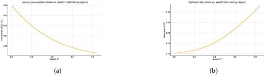
Figure 1.
Effects of luxury-specific ratcheting on consumption composition and portfolio choice. (a) Luxury consumption share as a function of wealth in the region where the luxury ratcheting constraint is binding. (b) Optimal risky share as a function of wealth in the same ratcheting region.
4. Conclusions
This paper studied an infinite-horizon optimal consumption and investment problem for an agent who consumes two types of goods—necessities and luxuries—under a ratcheting constraint on luxury consumption. The constraint prohibits any downward adjustment in luxury spending, capturing the behavioral feature that once a high living standard is achieved, it becomes psychologically or socially costly to reduce it. Using the dual–martingale approach, we transformed the primal problem into a dual formulation that further reduces to a sequence of optimal stopping problems. This structure enabled us to derive closed-form solutions for the value function, optimal consumption, and portfolio policies.
Our analysis shows that the ratcheting constraint generates asymmetric consumption dynamics. Necessity consumption adjusts smoothly in response to wealth changes, while luxury consumption exhibits strong downward rigidity. Consequently, the marginal propensity to consume necessities declines with wealth, and luxury spending dominates in the long run. The portfolio choice results demonstrate that the optimal risky share increases with wealth and exceeds the benchmark level without ratcheting, implying stronger risk-taking behavior among high-wealth individuals. These results provide an economic explanation for the persistence of high consumption levels and elevated risk exposure observed in wealthy households.
The model can be extended in several directions. One promising avenue is to introduce a finite planning horizon or incorporate stochastic labor income to analyze life-cycle implications of luxury ratcheting. Another extension is to relax the complete-markets assumption and study how limited risk sharing affects the interaction between luxury ratcheting and portfolio choice; we conjecture that in incomplete markets the ratcheting friction would further amplify precautionary saving and reduce effective risk sharing. A further direction is to consider general equilibrium effects when heterogeneous agents with different ratcheting intensities interact in financial markets. Such extensions would enhance our understanding of the interplay between consumption habits, inequality, and risk-taking behavior in dynamic economic environments.
From an empirical perspective, our model generates several testable implications. For instance, conditional on wealth, households with a higher past peak in luxury consumption should display stronger downward rigidity in luxury spending after negative shocks, and they should hold a larger share of risky assets to sustain their luxury standard. These predictions could be examined using panel data that track detailed consumption categories and portfolio allocations over time (such as CEX- or PSID-type data), and we leave a systematic empirical investigation to future work.
Author Contributions
Conceptualization, G.K.; Methodology, G.K.; Formal analysis, J.J.; Writing—original draft, J.J.; Writing—review and editing, J.J. All authors have read and agreed to the published version of the manuscript.
Funding
This research received no external funding.
Data Availability Statement
No new data were created or analyzed in this study.
Conflicts of Interest
The authors declare no conflicts of interest.
Abbreviations
The following abbreviations are used in this manuscript:
| Agent’s financial wealth at time t | |
| Consumption rate of the necessity good at time t | |
| Consumption rate of the luxury good at time t | |
| Luxury consumption level just before t (ratcheting reference) | |
| L | Shift parameter in the utility from luxury goods |
| Subjective discount rate | |
| Risk aversion parameter for the necessity good | |
| Risk aversion parameter for the luxury good | |
| Utility weight on the luxury good | |
| r | Risk-free interest rate |
| Price of the risky asset at time t | |
| Expected continuously compounded return on the risky asset | |
| Volatility of the risky asset | |
| Market price of risk, | |
| Dollar amount invested in the risky asset at time t | |
| State-price density (stochastic discount factor) | |
| Risk-adjusted discount rate for good i, | |
| Roots of the characteristic equation in Equation (8) | |
| Free-boundary level in the optimal stopping problem | |
| Primal value function | |
| Dual value function | |
| Value function of the optimal stopping problem |
References
- Merton, R.C. Lifetime portfolio selection under uncertainty: The continuous-time case. Rev. Econ. Stat. 1969, 51, 247–257. [Google Scholar] [CrossRef]
- Merton, R.C. Optimum consumption and portfolio rules in a continuous-time model. J. Econ. Theory 1971, 3, 373–413. [Google Scholar] [CrossRef]
- Duesenberry, J.S. Income, Saving, and the Theory of Consumer Behavior; Harvard University Press: Cambridge, MA, USA, 1949. [Google Scholar]
- Dybvig, P.H. Duesenberry’s ratcheting of consumption: Optimal dynamic consumption and investment given intolerance for any decline in standard of living. Rev. Econ. Stud. 1995, 62, 287–313. [Google Scholar] [CrossRef]
- Campbell, J.Y.; Cochrane, J.H. By force of habit: A consumption-based explanation of aggregate stock market behavior. J. Political Econ. 1999, 107, 205–251. [Google Scholar] [CrossRef]
- Carroll, C.D. Why do the rich save so much? In Does Atlas Shrug? The Economic Consequences of Taxing the Rich; Slemrod, J., Ed.; Harvard University Press: Cambridge, MA, USA, 2002; pp. 465–484. [Google Scholar]
- Aït-Sahalia, Y.; Parker, J.A.; Yogo, M. Luxury goods and the equity premium. J. Financ. 2004, 59, 2959–3004. [Google Scholar] [CrossRef]
- Wachter, J.A.; Yogo, M. Why do household portfolio shares rise in wealth? Rev. Financ. Stud. 2010, 23, 3929–3965. [Google Scholar] [CrossRef]
- Cox, J.C.; Huang, C.F. Optimal consumption and portfolio policies when asset prices follow a diffusion process. J. Econ. Theory 1989, 49, 33–83. [Google Scholar] [CrossRef]
- Peskir, G. The Russian option: Finite horizon. Financ. Stochastics 2005, 9, 251–267. [Google Scholar] [CrossRef]
- Blinder, A.S. Distribution effects and the aggregate consumption function. J. Political Econ. 1975, 83, 447–475. [Google Scholar] [CrossRef]
- Karatzas, I.; Shreve, S.E. Methods of Mathematical Finance; Springer: New York, NY, USA, 1998. [Google Scholar]
- Friend, I.; Blume, M.E. The demand for risky assets. Am. Econ. Rev. 1975, 65, 900–922. [Google Scholar]
- Mehra, R.; Prescott, E.C. The equity premium: A puzzle. J. Monet. Econ. 1985, 15, 145–161. [Google Scholar] [CrossRef]
- Rockafellar, R.T. Convex Analysis; Princeton University Press: Princeton, NJ, USA, 1997. [Google Scholar]

Disclaimer/Publisher’s Note: The statements, opinions and data contained in all publications are solely those of the individual author(s) and contributor(s) and not of MDPI and/or the editor(s). MDPI and/or the editor(s) disclaim responsibility for any injury to people or property resulting from any ideas, methods, instructions or products referred to in the content. |
© 2025 by the authors. Licensee MDPI, Basel, Switzerland. This article is an open access article distributed under the terms and conditions of the Creative Commons Attribution (CC BY) license (https://creativecommons.org/licenses/by/4.0/).