Software Reliability Growth Model Combining Testing Effort Function and Burr-Type Fault Detection Rate

Abstract

Software reliability growth models (SRGMs) often assume a linear relationship between the fault detection rate (FDR) and testing effort function (TEF), which fails to capture their dynamic and nonlinear characteristics. To address this limitation, this paper proposes a novel SRGM framework that employs Burr-III and Burr-XII distributions to characterize the FDR, integrated with S-shaped TEFs. To tackle the parameter estimation challenge for such complex models, we designed a hybrid GRU-HMM deep learning framework. Experiments on multiple real-world datasets demonstrate that the proposed models (particularly III-is and XII-is) significantly outperform traditional baseline models in both goodness-of-fit and prediction accuracy. Quantitatively, on the DS1 dataset, the III-is model reduced the MSE from 110.7 to 102.9 and improved the AIC from 108.3 to 91.7 compared to the best baseline. On the DS2 dataset, the XII-is model notably decreased the MSE from 64.2 to 48.9. These results not only validate the theoretical advantage of combining Burr distributions with S-shaped TEFs in modeling nonlinear, multi-phase testing dynamics but also provide a practical solution for high-precision reliability assessment and resource planning in complex software testing environments.

1. Introduction

Software testing constitutes an indispensable process that forms the foundation for guaranteeing software product quality and reliability. The absence of a systematic testing protocol would substantially impede software companies’ product release capabilities, given the potential repercussions of distributing defective software to end-users [1]. Accurate reliability evaluation before deployment is crucial for ensuring software quality and determining optimal release timing. Particularly in security-critical applications, SRGMs assume vital importance by enabling the forecasting of defect patterns and evaluating software reliability throughout the testing cycle [2].

SRGMs primarily function to characterize software fault manifestations and project future fault occurrence rates. Numerous SRGM variants have been developed to address complexities in modern systems. The foundational Goel–Okumoto model, which presumes a time-decreasing failure rate [3], demonstrates applicability during initial software lifecycle phases but reveals limitations in complex system environments. Subsequent innovations including the delayed S-shaped and inflection S-shaped models were conceived to overcome these constraints. Concurrently, scholarly contributions from Nagaraju et al. and Garg et al. have introduced enhanced software reliability frameworks tailored to diverse software operational contexts [4,5]. Sindhu advanced this domain through an refined Weibull model incorporating modified defect detection rates to accommodate operational uncertainties [6]. Yang further expanded the methodological spectrum by proposing an additive reliability framework employing stochastic differential equations for analyzing censored data in multi-component architectures [7].

The core challenge in SRGM development centers on effective modeling strategies that incorporate crucial factors such as fault dependency relationships, software module interactions, and test coverage metrics [8,9,10,11]. A particularly significant advancement in this domain involves the integration of testing effort function (TEF) into the modeling framework. The incorporation of TEF enables a comprehensive representation of resource utilization during testing phases and its consequential impact on fault detection efficiency [12]. Early research by Yamada characterized testing effort through Rayleigh and exponential curves [13], while Li and colleagues expanded this work by integrating both delayed and infected S-shaped TEFs into reliability growth modeling [14]. Subsequent developments include Dhaka’s implementation of exponential additive Weibull distribution as a testing effort function [15], and Kushwaha’s incorporation of Logistic testing effort functions within SRGM frameworks [16].

Despite these advancements, current methodologies frequently overlook the inherently dynamic nature of TEF, particularly failing to address how phase-specific variations in resource allocation influence both testing efficiency and fault detection rate (FDR). Many established models employ simplified TEF representations that primarily correlate with temporal progression or testing milestones [17], without adequately accounting for the distinctive resource consumption patterns across different testing phases. These simplistic representations limit the ability of conventional SRGMs to accurately capture the nonlinear and phase-dependent relationships between testing effort and fault detection in complex testing environments, representing a significant research gap that demands further investigation.

To bridge this methodological gap, we propose an innovative SRGM framework that simultaneously models the dynamic interplay between TEF and FDR. Our approach leverages Burr-XII and Burr-III distributions to characterize the evolving nature of FDR, enabling enhanced adaptability to the distinctive characteristics of various testing phases [18,19]. This formulation effectively captures the nuanced effects of resource consumption on fault detection capabilities. In contrast to traditional static modeling paradigms, our proposed framework explicitly accommodates temporal and phase-dependent variations in testing resource allocation, thereby providing more precise reliability assessment mechanisms for complex testing scenarios.

Following the proposal of a SRGM, parameter estimation constitutes the next critical step. It is vital for the model’s accuracy and effectiveness, as it directly impacts predictive capability and reliability assessment. Least squares estimation (LSE) [20,21] is a commonly employed method for this purpose. LSE estimates parameters by minimizing the sum of squared errors between predicted and observed values, making it suitable for linear models. However, with the increasing complexity of software systems, LSE becomes inadequate for handling nonlinear relationships [22]. Beyond traditional estimation methods, some studies have also explored the use of meta-heuristic optimization algorithms, such as genetic algorithms (GA) and particle swarm optimization (PSO), for estimating parameters in complex SRGMs [23]. Our GRU-HMM approach offers a distinct, deep learning-based alternative to these population-based optimization strategies.

Deep learning methods have emerged as a novel approach for parameter estimation in this context. For instance, Wu [24] proposed a framework for learning SRGM parameters through the weights of deep neural networks, essentially utilizing deep learning feedback mechanisms. Similarly, Kim [25] developed a software reliability model based on gated recurrent units (GRUs), replacing the activation functions used in prior deep learning models. Nevertheless, existing deep-learning-based SRGM modeling approaches exhibit significant limitations: they simplistically map SRGM expressions to the activation functions or hidden layer outputs of neural networks. This results in parameters that violate physical constraints, insufficient long-term prediction stability inherent to GRUs, and an inability to adapt to phase transitions in resource allocation ultimately leading to significant prediction volatility in complex scenarios.

To address these challenges and enhance estimation accuracy, we propose a hy-brid GRU-HMM method. This approach leverages the GRU’s proficiency in processing sequential data and the HMM’s capability in modeling discrete hidden states [26,27], thereby offering a more suitable framework for complex software reliability modeling.

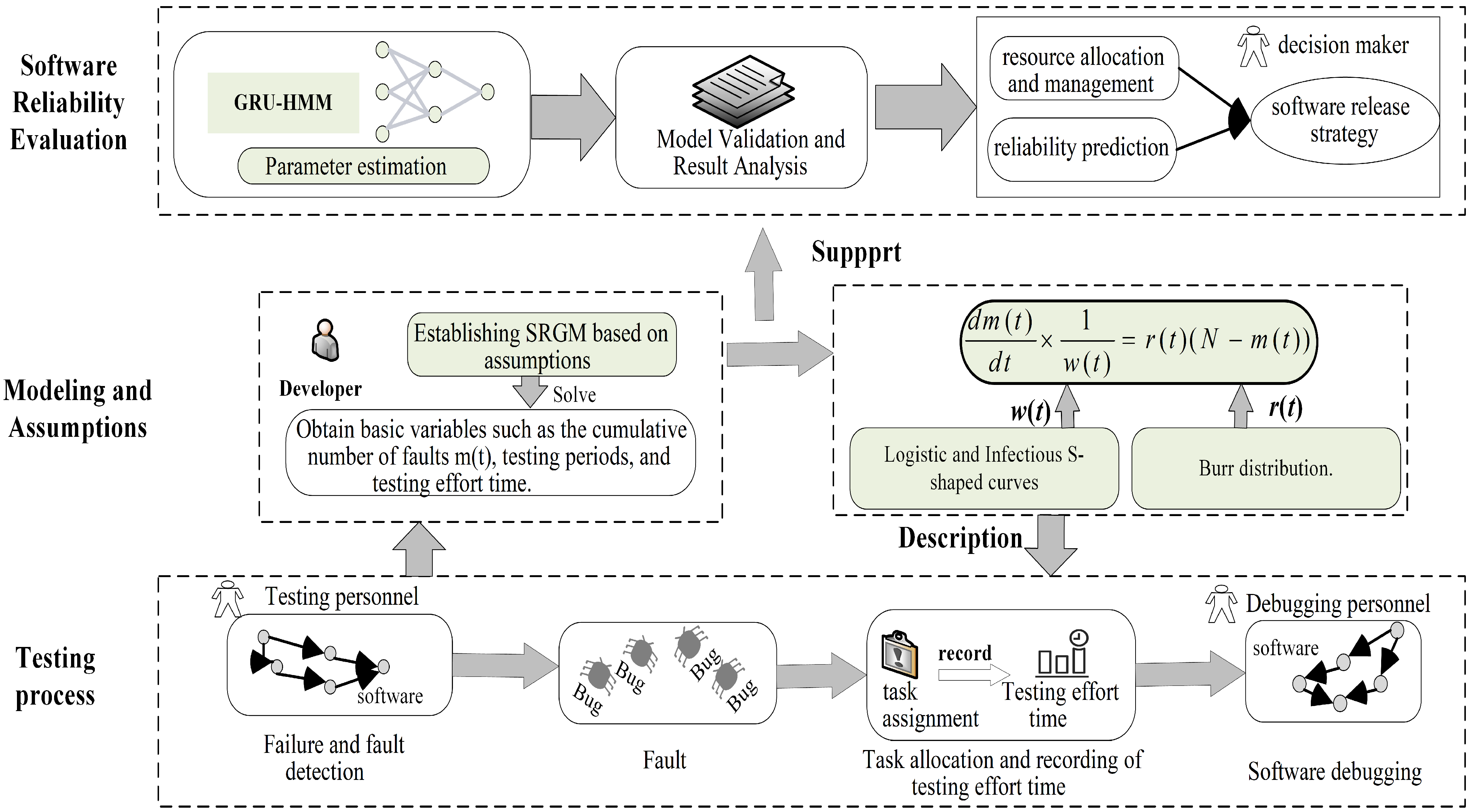
Figure 1 illustrates the basic process of SRGM modeling based on our understanding of the testing process, covering the testing process related to software reliability re-search, software reliability modeling, and their corresponding relationships. The high-lighted content in Figure 1 represents the core of this paper, focusing on two main aspects: reliability modeling and parameter estimation. The introduction outlines the research context and motivations. The related work section reviews SRGMs and relevant theoretical advancements. Section 2 presents the SRGM, Section 3 introduces the parameter estimation method, and Section 4 validates the model. Section 5 concludes the study and suggests future research directions.

Our paper offers three contributions to software reliability growth modeling:

• We propose a novel SRGM framework that integrates Burr-III and Burr-XII distributions with S-shaped testing effort functions to capture the nonlinear and phase-dependent dynamics of the fault detection rate.
• We design a hybrid GRU-HMM deep learning method for robust parameter estimation, effectively addressing the challenges of nonlinearity and phase transitions in complex testing environments.
• We conduct extensive empirical studies on real-world datasets, demonstrating that our proposed models significantly outperform traditional baselines in both goodness-of-fit and prediction accuracy.

2. Preliminaries

2.1. Software Reliability Growth Models

Software reliability growth models are statistical methods used to quantify the improvement of software reliability during testing and early operation [21]. The core idea is that as testing progresses, defects are discovered and removed, leading to a gradual enhancement of reliability.

SRGMs primarily rely on failure data collected during testing, such as inter-failure times or cumulative failure counts. The key objective is to estimate the mean value function and the failure intensity function to capture the system’s reliability evolution [28].

The theoretical foundation of most SRGM is the non-homogeneous Poisson process (NHPP), which assumes that the failure rate changes over time. As faults are fixed, the number of remaining defects decreases, leading to a decline in the failure rate.

2.2. Testing Effort Function

The testing effort function (TEF) is an important mathematical concept in software reliability modeling, used to characterize the distribution pattern of testing re-sources over time. It is defined as a non-negative, monotonically increasing function of time, reflecting how testing activities accumulate throughout the software lifecycle. Formally, TEF is typically denoted as W(t), where W(t) represents the testing time, and W(t) indicates the total amount of testing effort invested up to time t.

In software reliability growth models, the introduction of the testing effort function significantly enhances the model’s ability to represent realworld testing processes. Traditional SRGMs often assume a uniform testing intensity throughout the entire testing period. However, in practice, the allocation of testing resources usually varies over time, exhibiting non-uniform characteristics. For example, testing efforts may be minimal in the early stages of a project but increase sharply as the release deadline approaches. By incorporating TEF into SRGMs, time-driven models can be transformed into effort-driven models, allowing for a more accurate representation of the actual relationship between fault detection rates and testing input.

Mathematically, the testing effort function is typically used to replace the time variable t in traditional software reliability growth models, transforming the cumulative failure function (i.e., the mean value function) m(t) into m(W(t)). Specifically, the model becomes

$$m\left(t\right)=N(1-e^{-b}\times W\left(t\right)),$$

(1)

where N denotes the total number of potential faults in the system and b is the fault detection efficiency parameter.

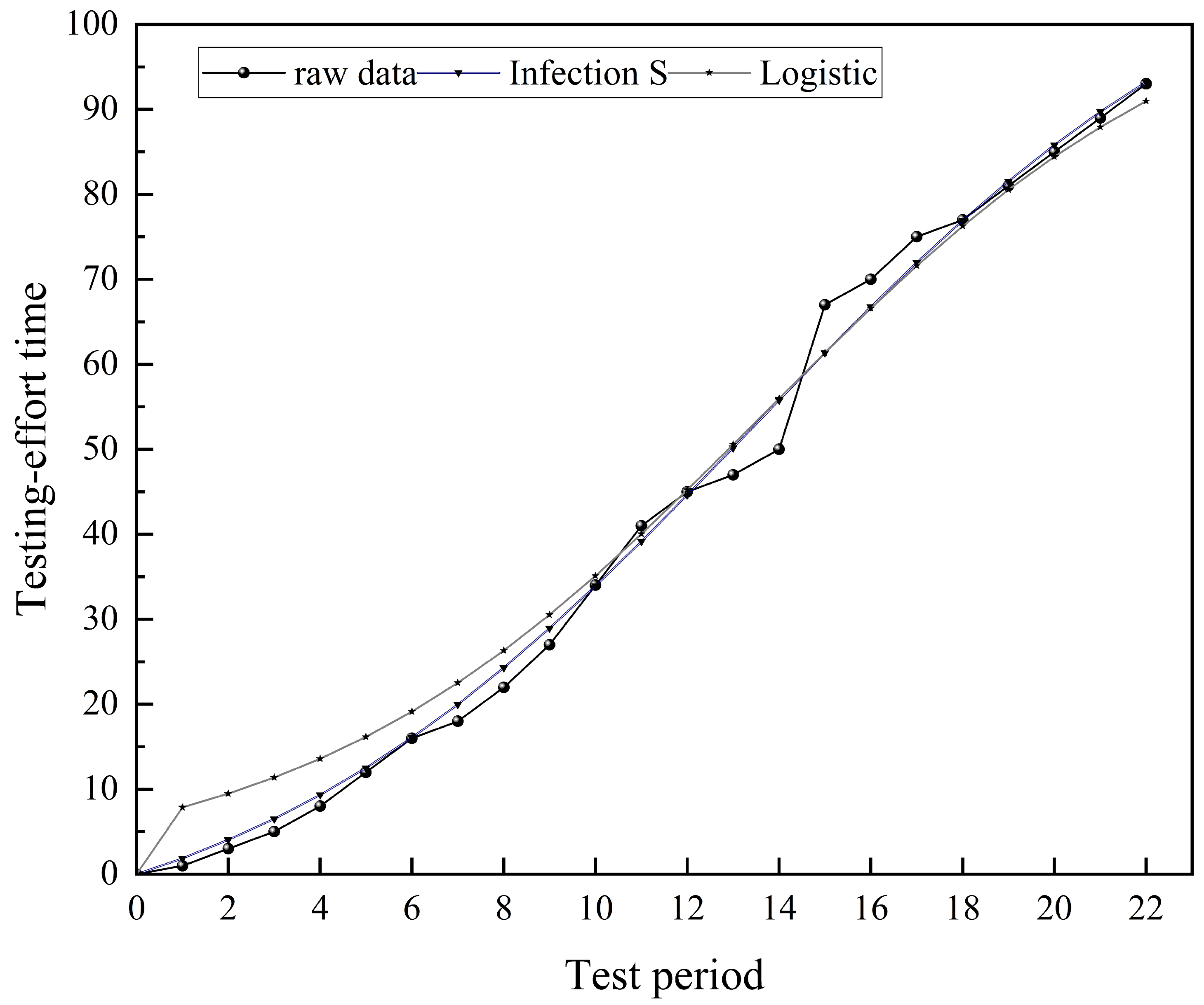
The testing effort function (TEF) is characterized by two distinct curve types: convex-type and S-type. Convextype TEFs emphasize aggressive early-stage resource allocation to maximize risk mitigation efficiency. Conversely, S-type TEFs model phased testing processes, reflecting incremental workload evolution from initial system configuration, through sustained regression validation, to eventual stabilization. This phased structure makes S-type TEFs particularly suitable for safety-critical systems, where workload dynamics must align with rigorous reliability requirements. The selection between these curves critically influences SRGM accuracy in simulating testing rhythms, enabling data-driven optimization of resource-reliability trade-offs.

Table 1. Growth Curve Functions and their expressions.

TEF	Type	$\mathit{W}\left(\mathit{t}\right)$	Reference
Exponential	concave	$W\left(t\right)=W_{max}(1-e^{-ct})$	[13]
Rayleigh	concave	$W\left(t\right)=W_{max}(1-e^{-c{t}^2})$	[16]
Weibull	S	$W\left(t\right)=W_{max}(1-e^{-c{t}^{\beta }})$	[6]
Infection S	S	$W\left(t\right)=W_{max}(1-e^{-ct}){(1+\phi e^{-ct})}^{-1}$	[14]
Logistic	S	$W\left(t\right)=W_{max}{(1+\phi e^{-ct})}^{-1}$	[14]

summarizes the key TEF variants examined in this study, including their mathematical formulation.

2.3. Burr Distribution

The Burr distribution is a flexible continuous probability distribution widely used in fields such as engineering, economics, medicine, and reliability analysis. Introduced by Burr in 1942 [29], it effectively fits various types of data. A key feature of the Burr distribution is its ability to model different tail behaviors by adjusting parameters, allowing it to represent multiple distribution forms. The Burr-III and Burr-XII distributions are widely used in SRGM due to their flexibility in modeling various failure patterns [18,19]. They effectively capture the dynamic changes in failure detection rates, and their ability to model both light-tailed and heavy-tailed behaviors improves the accuracy of SRGM predictions.

The effectiveness of Burr distributions in modeling software fault detection lies in their inherent flexibility to adapt to various testing phases, a feature not fully captured by traditional distributions like the Exponential or Weibull, which often assume a fixed failure pattern. The key advantage of Burr-III and Burr-XII distributions is their ability to model both light-tailed and heavy-tailed behaviors. This enables them to accurately represent the entire software testing lifecycle: initially capturing the slow detection rate of early testing phases, often due to team learning curves; then modeling the accelerated fault discovery during peak testing activity; and finally reflecting the saturation effect in later stages as the number of remaining faults diminishes. This multi-phase adaptability makes Burr distributions particularly suitable for modern software testing environments, where both the testing effort allocation and fault detection efficiency vary nonlinearly over time.

In software reliability modeling, the Burr-type fault detection rate is defined by its cumulative distribution function (CDF) and probability density function (PDF). The CDF quantifies the cumulative probability of detecting faults by time t, while the PDF, derived as the derivative of the CDF, characterizes the instantaneous probability density of fault detection at any specific time.

The CDF of the Burr-XII distribution are defined as

$$F\left(t\right)=1-{(1+t^b)}^{-k}.$$

(2)

The CDF of the Burr-III distribution are defined as

$$F\left(t\right)={(1+t^{-b})}^{-k}.$$

(3)

In the Burr distribution, the parameters b > 0 and k > 0 are shape parameters. The parameter k governs the distribution’s shape and tail thickness, while b primarily influences the overall morphology of the distribution, particularly determining its skewness.

The fault detection rate, denoted as r(t), can be expressed using the PDF f(t) as follows:

$$f\left(t\right)=dF\left(t\right)/dt,$$

(4)

where f(t) is the probability density function, and the fault detection rate r(t) can be expressed as

$$r\left(t\right)=f\left(t\right)/1-F\left(t\right).$$

(5)

Here, 1 $-F\left(t\right)$ represents the probability of undetected faults at time t, which corresponds to the proportion of remaining faults.

Based on this, the fault detection rate expressions for the Burr-XII and Burr-III distributions can be derived. The fault detection rate for the Burr-XII distribution is expressed as:

$$r\left(t\right)=bk{t}^{b-1}{(1+t^b)}^{-1}$$

(6)

Similarly, the fault detection rate for the Burr-III distribution is expressed as

$$r\left(t\right)={\displaystyle \frac{bk{t}^{-b-1}}{(1+t^{-b})({(1+t^{-b})}^k-1)}}.$$

(7)

3. Proposed Method

This chapter introduces the implementation process of the above methodology, beginning with a description of the SRGM model construction steps, followed by a detailed explanation of the parameter estimation technique, and finally presenting the application framework of the method in practical scenarios.

3.1. Software Reliability Modeling

To describe the dynamic process of software fault detection more accurately, this section proposes a novel software reliability growth model based on Burr-type fault detection rates and S-shaped test effort functions, under the following assumptions:

(1)

The occurrence of software faults and their subsequent elimination follow a non-homogeneous Poisson process, where the failure rate varies over time.

(2)

Software faults occur at random times, caused by the remaining faults in the system.

(3)

The ratio of the average number of faults detected during a specific time interval to the test effort expended is directly proportional to the number of remaining faults in the system.

(4)

The fault detection rate is a time-varying function, described by Burr-III and Burr-XII distributions.

(5)

The consumption of test resources is modeled using different types of S-shaped Test Effort Functions, such as the Infection S-type and the Logistic-type.

(6)

When a fault is detected, it is immediately eliminated, and no new faults are introduced.

Given that the failure intensity, which represents the number of failures occurring per unit time at time t, can be derived from the fundamental assumptions of the model, it is expressed as

$${\displaystyle \frac{\mathrm{d}m\left(t\right)}{\mathrm{d}t}}=\lambda \left(t\right).$$

(8)

The failure intensity is directly proportional to the remaining number of faults $N-m\left(t\right)$ in the software. The proportionality constant is the composite fault detection rate $w\left(t\right)·r\left(t\right)$, which accounts for both the testing effort consumption rate $w\left(t\right)$ and the inherent fault detection rate $r\left(t\right)$. The expression is as follows:

$${\displaystyle \frac{\mathrm{d}m\left(t\right)}{\mathrm{d}t}}=\lambda \left(t\right)=w\left(t\right)·r\left(t\right)·(N-m\left(t\right)).$$

(9)

To solve for the mean value function $m\left(t\right)$, we rearrange Equation (2) into a standard differential equation:

$$\mathrm{d}m\left(t\right)=w\left(t\right)r\left(t\right)(N-m(t\left)\right)\mathrm{d}t.$$

(10)

Solving this first-order linear differential equation with respect to $m\left(t\right)$:

$$\begin{array}{cc}\hfill {\displaystyle \frac{\mathrm{d}m\left(t\right)}{N-m\left(t\right)}}& =w\left(t\right)r\left(t\right)\mathrm{d}t,\hfill \end{array}$$

(11)

$$\begin{array}{cc}\hfill \int {\displaystyle \frac{\mathrm{d}m\left(t\right)}{N-m\left(t\right)}}& =\int w(t)r(t)\mathrm{d}t,\hfill \end{array}$$

(12)

$$\begin{array}{cc}\hfill -ln|N-m(t\left)\right|& =\int w(t)r(t)\mathrm{d}t+C,\hfill \end{array}$$

(13)

$$\begin{array}{cc}\hfill N-m\left(t\right)& =e^{-C}·e^{-\int w\left(t\right)r\left(t\right)\mathrm{d}t},\hfill \end{array}$$

(14)

$$\begin{array}{cc}\hfill m\left(t\right)& =N-C_1{e}^{-\int w\left(t\right)r\left(t\right)\mathrm{d}t},\hfill \end{array}$$

(15)

where $C_1=e^{-C}$ is the constant of integration.

Applying the initial condition $m\left(0\right)=0$,

$$\begin{array}{cc}\hfill 0& =N-C_1{e}^{-{\int }_0^{0}w\left(u\right)r\left(u\right)\mathrm{d}u},\hfill \end{array}$$

(16)

$$\begin{array}{cc}\hfill 0& =N-C_1·e^0,\hfill \end{array}$$

(17)

$$\begin{array}{cc}\hfill C_1& =N.\hfill \end{array}$$

(18)

Substituting back, we obtain the definite integral form of the mean value function:

$$m\left(t\right)=N\left(1-e^{-{\int }_0^{t}r\left(u\right)w\left(u\right)\mathrm{d}u}\right).$$

(19)

Beyond empirical metrics, the structural saturation behavior of an SRGM is a key theoretical property, often analyzed through the lens of Hausdorff saturation [30,31]. This property, for which two-sided estimates have been developed as a model selection criterion [32], describes the asymptotic bound of the mean value function.

The proposed framework demonstrates well-behaved saturation properties, anchored in its S-shaped testing effort function—which is inherently bounded and converges to a finite maximum—and the adaptable fault detection dynamics afforded by the Burr-type distribution. Under the non-homogeneous Poisson process (NHPP) assumption, these elements jointly ensure that the cumulative number of detected faults approaches a finite upper bound, consistent with established saturation theory. This structural coherence not only supports empirical robustness but also aligns with theoretical expectations formalized via Hausdorff saturation [30,31], where two-sided bounds serve as model selection criteria [32].

Existing NHPP-based SRGMs vary considerably in their assumptions and applicability. The Goel–Okumoto model, while simple and widely adopted, assumes constant fault detection and perfect debugging, neglecting early-stage inefficiencies and learning effects. The delayed S-Shaped model introduces a learning curve, better matching real-world fault accumulation trends, yet retains idealized debugging assumptions. The Yamada imperfect debugging model incorporates fault insertion during repairs, improving realism at the expense of parameter complexity. Similarly, the modified Weibull model introduces environmental variability via the Weibull distribution but faces challenges in parameter interpretation. The inflected S-shaped TEF model ties fault detection to effort saturation, though it presumes a consistent effort–detection relationship not always observed in practice.

These models collectively illustrate a persistent trade-off: enhanced realism often entails greater complexity and data requirements, whereas simpler models risk overlooking essential dynamics of the testing process. Our approach seeks a balanced integration of dynamic TEF and Burr-type FDR, maintaining theoretical grounding in saturation behavior while preserving practical estimability.

3.2. Parameter Estimation

This study introduces a hybrid GRU-HMM framework for robust parameter estimation in SRGMs, designed to overcome the limitations of traditional methods like LSE in capturing nonlinear and phase-varying fault dynamics. The GRU module acts as a temporal encoder, processing sequential testing data (e.g., CPU hours, defect counts) to model complex interactions between testing effort and failures. It is preferred over RNNs and LSTMs for its balance of gradient stability and computational efficiency. The derived latent features are then processed by an HMM, which models them as observations from discrete hidden states, each representing a distinct testing phase with a unique parameter set. By inferring transition probabilities between these states, the HMM dynamically adjusts parameters in response to shifts in testing strategy, ensuring alignment with actual processes. This coupling yields time-varying reliability models that preserve SRGMs’ analytical form while integrating data-driven dynamics. The framework is further regularized with domain knowledge to ensure physical plausibility and employs Monte Carlo dropout for uncertainty quantification, providing confidence intervals critical for release planning. The result is an accurate, interpretable, and adaptable tool for reliability assessment in complex testing environments.

GRU-HMM Architecture Design

The proposed architecture consists of two components: a GRU network for temporal feature extraction, and an HMM-based phase inference and parameter fusion module for multi-stage parameter estimation.

(1)

GRU Temporal Encoder

The GRU computes the hidden state at time step t using the following equations. Given the normalized input sequence: ${\mathbf{x}}_t\in \mathbb{R}$ (e.g., test effort or observed failures), the GRU network processes the sequence to generate a hidden state ${\mathbf{h}}_t$ as follows:

$$\begin{array}{cc}\hfill r_t& =\sigma (W_r·[h_{t-1},x_t]+b_r),\hfill \end{array}$$

(20)

$$\begin{array}{cc}\hfill z_t& =\sigma (W_z·[h_{t-1},x_t]+b_z),\hfill \end{array}$$

(21)

$$\begin{array}{cc}\hfill g_t& =tanh(W_g·[r_t·h_{t-1},x_t]+b_g),\hfill \end{array}$$

(22)

$$\begin{array}{cc}\hfill h_t& =(1-z_t)·g_t+z_t·h_{t-1},\hfill \end{array}$$

(23)

where ${\mathbf{h}}_t$ is the hidden state at the current time step, ${\mathbf{x}}_t$ is the input data at the current time step, $r_t$ and $z_t$ are the outputs of the reset gate and update gate respectively, and ${\mathbf{g}}_t$ is the candidate hidden state.

(2)

HMM Inference Module

The output sequence $h_{1:T}$ is modeled as observations of an HMM with a discrete hidden state set: $S=\{1,2,3,\dots ,K\}$, corresponding to latent test phases. Each hidden state $s_t=k$ is associated with a distinct SRGM parameter vector:

$${\theta }^{\left(k\right)}=[W_{\max }^{\left(k\right)},b^{\left(k\right)},{\phi }^{\left(k\right)},N^{\left(k\right)},c^{\left(k\right)},{\kappa }^{\left(k\right)}].$$

(24)

Note: The parameter ${\kappa }^{\left(k\right)}$ denotes the shape parameter of the Burr distribution, distinguished from the hidden state index k.

The hidden state process is modeled as a discrete-time hidden Markov model defined by

• Initial state distribution: ${\pi }_k=P(s_1=k)$, where ${\sum }_{k=1}^K{\pi }_k=1;$
• State transition probabilities: $A_{ij}=P(s_t=j|s_{t-1}=i)$, forming the transition matrix $A\in {\mathbb{R}}^{K\times K}$ with ${\sum }_{j=1}^K{A}_{ij}=1$ for all i.

The emission distribution links the continuous GRU-generated latent features $h_t\in {\mathbb{R}}^d$ to the discrete hidden states $s_t$. We assume this follows a multivariate Gaussian distribution:

$$p\left(h_t\right|s_t=k)=\mathcal{N}(h_t;{\mu }_k,{\Sigma }_k),$$

(25)

where ${\mu }_k\in {\mathbb{R}}^d$ is the mean vector and ${\Sigma }_k=\mathrm{diag}({\sigma }_{k,1}^2,\dots ,{\sigma }_{k,d}^2)$ is a diagonal covariance matrix. Both ${\mu }_k$ and ${\sigma }_k^2$ are learnable parameters representing the distribution characteristics of the GRU hidden states conditioned on hidden state k.

To compute the posterior state probabilities ${\gamma }_t^{\left(k\right)}$, we employ the forward–backward algorithm:

Forward Pass: Compute the forward probabilities ${\alpha }_t\left(k\right)=P(h_{1:t},s_t=k)$ recursively:

$$\begin{array}{cc}\hfill {\alpha }_1\left(k\right)& ={\pi }_k·p\left(h_1\right|s_1=k),\hfill \end{array}$$

(26)

$$\begin{array}{cc}\hfill {\alpha }_t\left(k\right)& =p\left(h_t\right|s_t=k)\sum _{j=1}^K{\alpha }_{t-1}\left(j\right)A_{jk}\mathrm{for}t=2,\dots ,T.\hfill \end{array}$$

(27)

Backward Pass: Compute the backward probabilities ${\beta }_t\left(k\right)=P\left(h_{t+1:T}\right|s_t=k)$ recursively:

$$\begin{array}{cc}\hfill {\beta }_T\left(k\right)& =1,\hfill \end{array}$$

(28)

$$\begin{array}{cc}\hfill {\beta }_t\left(k\right)& =\sum _{j=1}^K{A}_{kj}·p\left(h_{t+1}\right|s_{t+1}=j)·{\beta }_{t+1}\left(j\right)\mathrm{for}t=T-1,\dots ,1.\hfill \end{array}$$

(29)

Using these computed forward and backward probabilities, the posterior state probability at each time step is given by

$${\gamma }_t^{\left(k\right)}=P(s_t=k|h_{1:T})={\displaystyle \frac{{\alpha }_t\left(k\right){\beta }_t\left(k\right)}{{\sum }_{j=1}^K{\alpha }_t\left(j\right){\beta }_t\left(j\right)}}.$$

(30)

This posterior represents the probability of being in state k at time t, given all observed GRU features $h_{1:T}$. The denominator ensures proper normalization across all possible states.

The parameters of the HMM (initial distribution $\pi$, transition matrix A, and emission parameters ${\mu }_k,{\sigma }_k$) are learned jointly with the GRU parameters through backpropagation, maximizing the likelihood of the observed sequence $h_{1:T}$.

(3)

Parameter Fusion and SRGM Construction

The posterior state distribution ${\gamma }_t^{\left(k\right)}$ obtained from the HMM inference module is utilized to compute a time-varying parameter vector through weighted fusion:

$${\theta }_t=\sum _{k=1}^K{\gamma }_t^{\left(k\right)}{\theta }^{\left(k\right)},$$

(31)

where ${\theta }^{\left(k\right)}$ represents the SRGM parameter vector associated with hidden state k, as defined in Equation (17).

The fused parameters ${\theta }_t$ are substituted into analytical SRGM equations to compute test effort functions $w_t$, detection rate $r\left(t\right)$, and the cumulative failure mean function $m\left(t\right)$.

3.3. Loss Function and Optimization

To train the model, the predicted cumulative fault count $\widehat{m}\left(t\right)$ is compared with the actual observed value $m\left(t\right)$, and the mean squared error is used as the loss function:

$$L={\displaystyle \frac{1}{T}}\sum _{t=1}^T{[\widehat{m}\left(t\right)-m\left(t\right)]}^2.$$

(32)

The entire network is trained end-to-end using the Adam optimizer, with joint optimization of parameters across multiple components. These include

• Weights of the GRU network;
• Initial state distribution $\pi$ and state transition matrix A of the HMM;
• Gaussian emission parameters ${\mu }_k$ and ${\sigma }_k$ for each hidden state;
• SRGM parameter set ${\theta }^{\left(k\right)}$ for each latent state k.

This enables dynamic estimation of multi-phase software reliability model parameters.

3.4. Innovation: Adaptive Regularization and Uncertainty Quantification

To enhance estimation robustness and quantify predictive confidence, we introduce two key improvements:

3.4.1. Physics-Informed Adaptive Regularization

We augment the loss function with domain-driven regularization terms:

$$L_{\mathrm{reg}}=L+{\lambda }_1\sum _k{\parallel {\theta }_k-{\theta }_{\mathrm{prior}}\parallel }^2+{\lambda }_2\sum _{t}max(0,-r\left(t\right)),$$

(33)

where ${\theta }_{\mathrm{prior}}$ represents empirical parameter bounds derived from historical data. The second term enforces non-negativity of the fault detection rate. Hyperparameters ${\lambda }_1$ and ${\lambda }_2$ are optimized via Bayesian optimization.

3.4.2. Monte Carlo Dropout for Uncertainty Quantification

We implement dropout within GRU layers and perform M stochastic forward passes during inference:

$${\widehat{m}}^{\left(i\right)}\left(t\right)=f_{\mathrm{SRGM}}(x_t;{\theta }_t^{\left(i\right)}),i=1,\dots ,M.$$

(34)

The final prediction is obtained by averaging over the Monte Carlo samples:

$$\mathbb{E}\left[m\left(t\right)\right]={\displaystyle \frac{1}{M}}\sum _{i=1}^M{\widehat{m}}^{\left(i\right)}\left(t\right).$$

(35)

Prediction intervals are constructed using the empirical quantiles of the Monte Carlo samples.

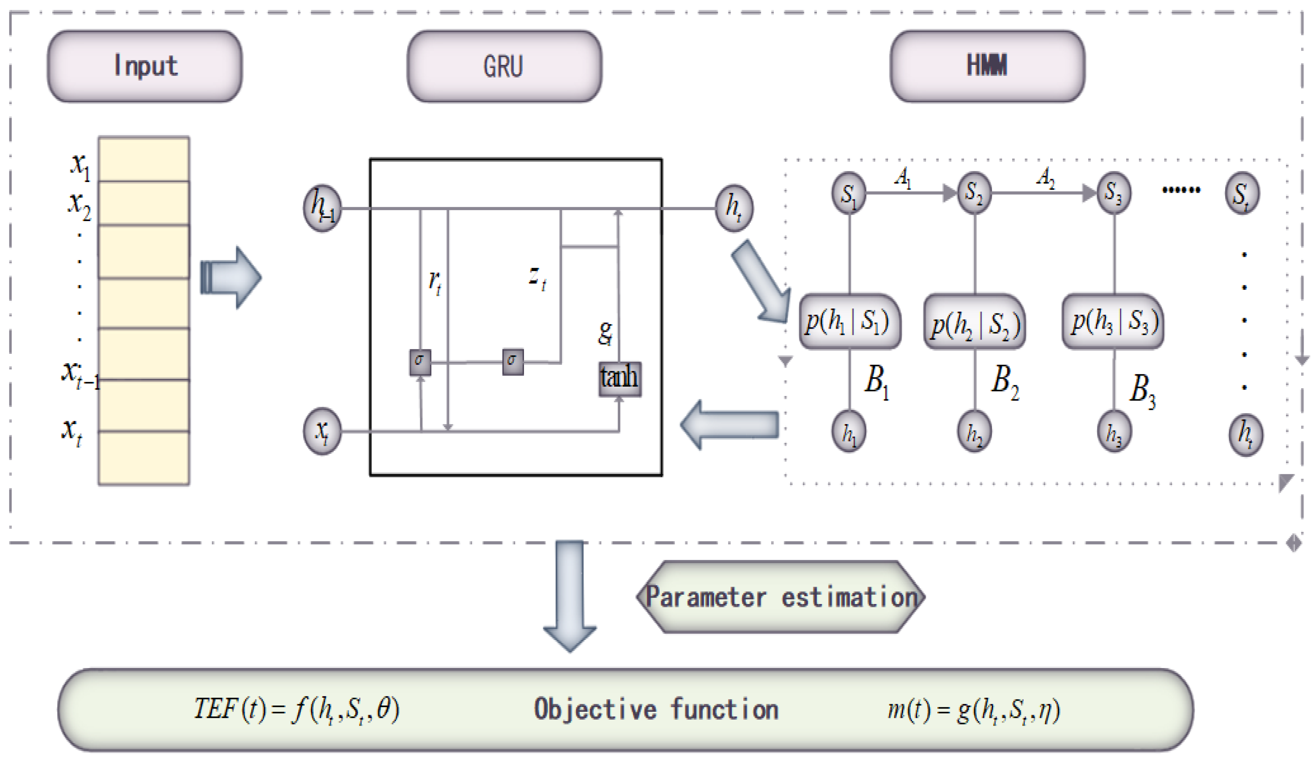
Figure 2 illustrates the multi-stage workflow of the GRU-HMM framework for constructing the SRGM. The process begins with the input of sequential testing data. This data is first processed by a Gated Recurrent Unit network to capture temporal dependencies and extract relevant features. Subsequently, a Hidden Markov Model analyzes these features to infer the latent phases of the software testing process. Finally, the framework integrates the outputs through a dynamic parameter fusion mechanism to accurately estimate the parameters of the SRGM.

4. Empirical Studies

4.1. Comparison Models and Evaluation Criteria

4.1.1. Comparison Models and Evaluation Criteria

To assess the fit and prediction performance of the proposed model, this experiment conducts a comprehensive analysis through comparisons in three aspects: the comparison of TEF selection, the comparison of parameter estimation methods, and the comparison of SRGMs. These comparisons help to gain a deeper understanding of how each component performs in different experimental scenarios and how they collectively influence the overall performance of the proposed model. This paper selects five curves from

Table 2. Summary of Existing and Proposed SRGMs Incorporating Burr Distributions.

Model	$\mathit{r}\left(\mathit{t}\right)$	$\mathbf{TEF}\left(\mathit{W}\right(\mathit{t}\left)\right)$	$\mathit{m}\left(\mathit{t}\right)$	Reference
G-O	$r\left(t\right)=b$	−	$m\left(t\right)=N(1-e^{-bt})$	[3]
Delayed-S-shaped- Model	$r\left(t\right)={\displaystyle \frac{b^{2}t}{bt+1}}$	−	$m\left(t\right)=N(1-(1+bt)e^{-bt})$	[12]
Yamada imperfect-debugging	$r\left(t\right)=b$	−	$m\left(t\right)={\displaystyle \frac{Nb}{b+\alpha }}(e^{\alpha t}-e^{-bt})$	[34]
modified-Weibull	$r\left(t\right)=k+\alpha b{t}^{b-1}$	−	$m\left(t\right)=N\left(1-{\displaystyle \frac{W_{max}}{W_{max}+b{t}^a{e}^{\phi t}}}\right)$	[6]
SRGM-with-Inflected-S-shaped-TEF	$r\left(t\right)=b$	$W\left(t\right)=W_{max}(1-e^{-\alpha t}){(1+\phi e^{-\alpha t})}^{-1}$	$m\left(t\right)=N\left(1-e^{-{\displaystyle \frac{1-e^{-\alpha t}}{1+\phi e^{-\alpha t}}}}\right)$	[35]
III-is	$r\left(t\right)={\displaystyle \frac{bk{t}^{k-1}}{(1+t^k)({(1+t^k)}^c-1)}}$	$W\left(t\right)=W_{max}(1-e^{-\alpha t}){(1+\phi e^{-\alpha t})}^{-1}$	$m\left(t\right)=N\left(1-e^{-bk{\int }_0^t{\displaystyle \frac{s^{k-1}W\left(s\right)}{(1+s^k)({(1+s^k)}^c-1)}}ds}\right)$	proposed 1
III-LS	$r\left(t\right)={\displaystyle \frac{bk{t}^{k-1}}{(1+t^k)({(1+t^k)}^c-1)}}$	$W\left(t\right)=W_{max}(1-e^{-\alpha t}){(1+\phi e^{-\alpha t})}^{-1}$	$m\left(t\right)=N\left(1-e^{-bk{\int }_0^t{\displaystyle \frac{s^{k-1}W\left(s\right)}{(1+s^k)({(1+s^k)}^c-1)}}ds}\right)$	proposed 2
XII-is	$r\left(t\right)=bk{t}^{k-1}{(1+t^k)}^{-c-1}$	$W\left(t\right)=W_{max}{(1+\phi e^{-\alpha t})}^{-1}$	$m\left(t\right)=N\left(1-e^{-{\int }_0^{t}bk{s}^{k-1}{(1+s^k)}^{-c-1}W\left(s\right)ds}\right)$	proposed 3
XII-LS	$r\left(t\right)=bk{t}^{k-1}{(1+t^k)}^{-c-1}$	$W\left(t\right)=W_{max}{t}^a{e}^{-\beta t}$	$m\left(t\right)=N\left(1-e^{-{\int }_0^{t}bk{s}^{k-1}{(1+s^k)}^{-c-1}W\left(s\right)ds}\right)$	proposed 4

to describe the testing effort and conducts experimental validation on the SRGM models in

Table 3. Parameter Estimation and Performance Evaluation of Test–Effort Functions on DS1 and DS2.

Datasets	TEF	${\mathit{W}}_{\mathbf{max}}$	c	$\mathit{\phi }$	${\mathit{R}}^2$	MSE
DS1	Exponential	224.1	0.01	-	0.9650	5.08
	Rayleigh	49.1	0.007	-	0.9662	5.14
	Weibull	89.2	0.01	1.33	0.9872	2.13
	Infection	92.3	0.09	3.18	0.9957	0.82
	Logistic	53.8	0.002	6.31	0.9914	1.62
DS2	Exponential	1620.7	0.0006	-	0.9903	13.00
	Rayleigh	133.2	0.0001	-	0.9804	28.16
	Weibull	174.0	1.50	1.11	0.9931	9.69
	Infection	207.6	0.01	3.71	0.9981	2.58
	Logistic	142.5	0.03	14.1	0.9938	8.84

. The parameter estimation methods, LSE and GRU, are used as comparison benchmarks. LSE is a commonly used parameter estimation method, widely applied in regression analysis and model fitting [33]. The basic idea of LSE is to estimate the model parameters by minimizing the sum of the squared differences between the model’s predicted values and the actual observed values. The GRU model method proposed by Kim differs from traditional SRGMs in that it replaces the activation function in deep learning with a software reliability function resembling the shape of the Sigmoid function, thereby achieving the prediction effect of SRGMs [25].

4.1.2. Evaluation Criteria

To compare the performance of the models, the following evaluation indicators were chosen: Akaike information criterion (AIC), R-squared (R²), and mean squared error (MSE).

(1) AIC (Akaike information criterion)is the measure of model goodness and is defined as $\mathrm{AIC}=2K-2log\left(L\right)$, where K is the number of parameters and L is the maximum likelihood value. When the errors follow a normal distribution, it follows that

$$\mathrm{AIC}=2K+mlog\left({\displaystyle \frac{\mathrm{RSS}}{m}}\right),$$

(36)

where m is the sample size and $\mathrm{RSS}$ is the sum of squared residuals. A smaller value means a better model.

(2) $R^2$ (coefficient of determination) is a measure of the proportion of the variance in the dependent variable that is explained by the model. It is defined as

$$R^2=1-{\displaystyle \frac{\mathrm{RSS}}{\mathrm{TSS}}},$$

(37)

where $\mathrm{RSS}$ is the residual sum of squares and $\mathrm{TSS}$ is the total sum of squares. The value of $R^2$ ranges from 0 to 1, with a higher value indicating that the model explains more variance.

(3) MSE: mean squared error, the smaller the error the better the fit. It is defined as

$$\mathrm{MSE}={\displaystyle \frac{{\sum }_{j=1}^m{\left(m\left(t_j\right)-m_j\right)}^2}{m-p}},$$

(38)

where $m\left(t_j\right)$ denotes the estimate of cumulative number of failures at time $t_j$, $m_j$ denotes the cumulative number of failures observed at time $t_j$, m is the number of observations, and p is the number of parameters in the model.

(4) MAE: mean absolute error, the smaller the error the better the fit. It is defined as

$$\mathrm{MAE}={\displaystyle \frac{{\sum }_{j=1}^m\left|m\left(t_j\right)-m_j\right|}{m-p}},$$

(39)

where $m\left(t_j\right)$ denotes the estimate of cumulative number of failures at time $t_j$, $m_j$ denotes the cumulative number of failures observed at time $t_j$, m is the number of observations, and p is the number of parameters in the model.

To ensure a more robust and generalizable evaluation of the models, we employed five-fold cross-validation in addition to the standard train-test split. The dataset is randomly partitioned into five equal-sized folds. In each iteration, four folds are used for training (parameter estimation) and one fold is used for testing. This process is repeated five times, with each fold used exactly once as the test set. The final performance metrics reported are the mean and standard deviation across all five test folds. This approach provides a more reliable estimate of model performance and reduces the variance associated with a single random train-test split.

4.2. Failure Data

To ensure the comparability and consistency of our research, we conducted a comprehensive literature review through databases such as IEEE Xplore and observed that most existing studies consistently adopt several classic software reliability datasets [35,36,37]. The sample size (i.e., the number of time intervals or data points) in these classic datasets is typically in the tens to a hundred, which is a common standard in the field of software reliability modeling [28]. This is because collecting high-frequency, long-term failure data from industrial projects is challenging and costly. The selection of these established datasets allows for direct comparison with prior work and ensures that our models are evaluated on realistic, industry-recognized benchmarks.

Furthermore, to ensure data quality and the robustness of our analysis, we implemented a rigorous data preprocessing pipeline that included outlier detection. We employed the interquartile range (IQR) method, where any data point falling below $Q1-1.5\times IQR$ or above $Q3+1.5\times IQR$ was flagged as a potential outlier. Here, $Q1$ and $Q3$ are the first and third quartiles, respectively, and $IQR=Q3-Q1$. For the flagged potential outliers, we conducted a manual review to determine if they represented genuine anomalous behavior (e.g., a week with zero testing effort due to a holiday) or data recording errors. In our datasets (DS1 and DS2), no data points were identified as erroneous outliers requiring removal; all observed variations were deemed to be part of the natural testing process. This process ensures that our model is trained on authentic data patterns without introducing bias through arbitrary removal of valid data points.

The first employed dataset (DS1) was proposed for a PL/I database application software system consisting of approximately 1,317,000 LOC [38]. Over the course of 19 weeks (i.e., 19 data points), 47.65 CPU hours were consumed, and 328 software faults were removed. The DS2 dataset is derived from a long-term software testing process collected by Xiao [39], covering Bugzilla data from three successive versions of Firefox 3.0, 3.5, and 3.6. This dataset includes 131 weeks of testing time (i.e., 131 data points), significantly larger than the first dataset. During these 131 weeks, a total of 149 defects were identified.

Given the limited scale of our datasets (DS1, DS2) and the high expressiveness of the GRU-HMM model, we implemented a comprehensive strategy to prevent overfitting and ensure generalization: (1) early stopping monitored on a validation set; (2) Monte Carlo dropout within GRU layers as a Bayesian regularizer; and (3) physics-informed adaptive regularization to constrain parameters. These measures collectively ensured robust generalization while maintaining model performance, as evidenced by our experimental results.

4.3. Experimental Results and Analysis

4.3.1. Research Question 1: Which Curve Is Suitable for Describing the Testing Effort?

TEF describes the variation of testing effort over time, and an accurate TEF model is crucial for software reliability analysis and resource management. In this context, “TE” represents Testing Effort, with specific units: for DS1, it is measured in CPU hours, representing actual computational resources consumed; for DS2, it is measured in weeks, representing the calendar time invested in testing. Studies show that testing effort typically follows a nonlinear growth pattern, where S-shaped curves like Infection S and Logistic better capture this process. This paper fits these two S-shaped TEFs and three concave TEFs to real-world failure datasets and evaluates their performance using goodness-of-fit metrics to verify the suitability of S-shaped curves for TEF modeling. Table 2 presents the parameter estimation results and evaluation metrics for the selected Test Effort Functions fitted to datasets DS1 and DS2. Figure 3 and Figure 4, respectively, depict the curves of the Logistic and Infection S test effort functions, while also displaying the original data points to illustrate the relationship between the testing period and test effort.

As shown in Table 3, the Infection S and Logistic models perform excellently in both the DS1 and DS2 datasets. In the DS1 dataset, the Infection S model has an R² value of 0.9957 and an MSE of 0.82, while the Logistic model has an R² value of 0.9914 and an MSE of 1.62. Both models show very high fit and low prediction errors, effectively capturing the nonlinear saturation trend of CPU time consumption. For the DS2 dataset, the Infection S model has an R² value of 0.9981 and an MSE of 2.58, while the Logistic model has an R² value of 0.9938 and an MSE of 8.84, demonstrating high explanatory power and small errors. Although the Weibull curve is also an S-shaped curve, our experimental validation shows that it is less accurate than the Logistic and infectious S-shaped curves in describing testing effort.

As shown in Figure 3 (DS1) and Figure 4 (DS2), the predicted curves of the Infection S and Logistic models closely align with the original CPU hour consumption data. The near-overlap of the three curves during mid-to-late testing stages visually confirms the models’ accuracy in capturing the nonlinear growth and saturation trends of resource consumption. This tight fit not only validates the quantitative conclusions from earlier analysis—R² approaching 1 and extremely low MSE but also demonstrates the models’ ability to reconstruct the dynamic evolution of resource consumption: a characteristic S-shaped process from rapid accumulation to stabilized saturation.

4.3.2. Research Question 2: How to Compare the Performance of Different Parameter Estimation Methodsin SRGM?

This research question aims to systematically evaluate and compare the efficacy of different parameter estimation paradigms for software reliability growth models. We examine three distinct methodologies: the conventional least squares estimation, a standalone Gated Recurrent Unit network, and our novel hybrid GRU-HMM framework. This comparative design not only benchmarks contemporary deep learning approaches against a traditional statistical method but, more importantly, isolates and highlights the specific contribution of incorporating a hidden Markov model for phase-aware modeling. To ensure methodological rigor and generalizability, a five-fold cross-validation strategy was employed across two real-world datasets, DS1 and DS2, representing different project scales and testing contexts. Model performance was assessed using a comprehensive set of metrics—mean squared error, mean absolute error, and Akaike information criterion (AIC)—which collectively evaluate prediction accuracy, model fit, and parsimony.

The consolidated results, detailed in

Table 4. Parameter Estimation and Performance Evaluation of the SRGM Model on the DS1 Dataset (Five-Fold Cross-Validation Results).

NO	SRGM	Methods	Parameter Estimation	MSE	MAE	AIC
1	Goel–Okumoto	LSE	$N=760.5,b=0.03$	142.3	9.5	98.5
2	Delayed S-shaped	LSE	$N=374.0,b=0.19$	171.2	11.1	102.8
3	Yamada imperfect debugging	LSE	$N=372.7,b=0.001,c=0.93$	121.8	8.4	101.6
4	Modified Weibull	LSE	$N=299.9,b=0.07,c=0.01$, $W_{max}=9.72,k=0.07,\phi =0.19$	151.9	10.1	108.3
5	SI	LSE	$N=356.3,b=0.12,c=0.12$, $W_{max}=62.0,\phi =2.79$	112.7	8.2	106.9
6	Goel–Okumoto	GRU	$N=747.8,b=0.03$	142.8	9.6	107.5
7	Delayed S-shaped	GRU	$N=374.0,b=0.19$	171.2	11.1	102.8
8	Yamada imperfect debugging	GRU	$N=483.6,b=0.01,c=0.05$	150.4	9.9	101.7
9	Modified Weibull	GRU	$N=320.5,b=0.12,c=0.01$, $W_{max}=18.32,k=0.12,\phi =8.21$	114.7	8.3	107.1
10	SI	GRU	$N=578.8,b=0.22,c=0.01$, $W_{max}=54.8,\phi =13.03$	109.6	8.1	96.4
11	Goel–Okumoto	GRU-HMM	$N=760.5,b=0.03$	142.3	9.5	98.5
12	Delayed S-shaped	GRU-HMM	$N=374.0,b=0.19$	171.2	11.1	102.8
13	Yamada imperfect debugging	GRU-HMM	$N=328.1,b=0.001,c=0.21$	110.9	7.9	94.3
14	Modified Weibull	GRU-HMM	$N=631.1,b=0.15,c=0.14$, $W_{max}=9.40,k=0.11,\phi =1.70$	117.9	8.4	103.4
15	SI	GRU-HMM	$N=311.6,b=0.12,c=1.10$, $W_{max}=58.6,\phi =16.71$	108.4	7.8	98.6
16	XII-LS	GRU-HMM	$N=2302,b=0.09,c=0.83$, $W_{max}=92.3,k=0.03,\phi =3.18$	135.8	8.8	111.2
17	XII-is	GRU-HMM	$N=6538,b=0.23,c=0.88$, $W_{max}=53.8,k=0.01,\phi =13.8$	106.5	7.7	92.8
18	III-LS	GRU-HMM	$N=1574,b=0.09,c=0.30$, $W_{max}=92.3,k=6.75,\phi =3.18$	137.1	9.3	100.5
19	III-is	GRU-HMM	$N=1926,b=0.23,c=0.18$, $W_{max}=53.8,k=4.38,\phi =13.8$	102.9	7.5	91.7

and

Table 5. Parameter Estimation and Performance Evaluation of the SRGM Model on the DS2 Dataset (Five-Fold Cross-Validation Results).

NO	SRGM	Methods	Parameter Estimation	MSE	MAE	AIC
1	Goel–Okumoto	LSE	$N=247.1,b=0.007$	64.2	6.8	548.9
2	Delayed S-shaped	LSE	$N=159.2,b=0.032$	129.5	9.2	641.3
3	Yamada-imperfect-debugging	LSE	$N=205.4,b=0.001,c=0.009$	64.5	6.9	551.2
4	modified-Weibull	LSE	$N=607.5,b=0.003,c=0.03$, $W_{max}=7.63,k=3.25,\phi =1.99$	66.1	7.1	561.4
5	SI	LSE	$N=272.0,b=0.006,c=0.03$, $W_{max}=141.9,\phi =11.1$	84.3	7.9	589.8
6	Goel–Okumoto	GRU	$N=233.8,b=0.007$	83.2	8.1	588.5
7	Delayed S-shaped	GRU	$N=159.2,b=0.032$	129.5	9.2	641.3
8	Yamada imperfect debugging	GRU	$N=412.6,b=0.012,c=0.12$	124.1	9.8	616.2
9	Modified Weibull	GRU	$N=201.3,b=0.012,c=0.08$, $W_{max}=12.3,k=8.21,\phi =6.21$	236.8	13.5	1348.2
10	SI	GRU	$N=252.1,b=0.006,c=0.07$, $W_{max}=141.9,\phi =6.82$	79.2	7.6	564.7
11	Goel–Okumoto	GRU-HMM	$N=247.1,b=0.007$	64.2	6.8	548.9
12	Delayed S-shaped	GRU-HMM	$N=159.2,b=0.032$	129.5	9.2	641.3
13	Yamada imperfect debugging	GRU-HMM	$N=372.7,b=0.001,c=0.93$	61.9	6.5	546.1
14	Modified Weibull	GRU-HMM	$N=329.1,b=0.01,c=0.08$, $W_{max}=8.92,k=6.31,\phi =2.31$	62.0	6.6	544.8
15	SI	GRU-HMM	$N=262.1,b=0.006,c=0.03$, $W_{max}=141.9,\phi =11.11$	73.2	7.3	571.4
16	XII-LS	GRU-HMM	$N=783.1,b=0.03,c=1.51$, $W_{max}=142.5,k=0.03,\phi =14.1$	84.5	8.0	592.7
17	XII-is	GRU-HMM	$N=523.1,b=0.006,c=1.35$, $W_{max}=141.9,k=0.02,\phi =9.82$	48.9	5.2	481.3
18	III-LS	GRU-HMM	$N=631.2,b=0.03,c=0.37$, $W_{max}=142.5,k=8.31,\phi =14.1$	64.0	6.7	545.5
19	III-is	GRU-HMM	$N=952.1,b=0.006,c=0.27$, $W_{max}=141.9,k=6.52,\phi =9.78$	54.9	5.8	530.1

, reveal a clear hierarchy in performance. For simpler model structures like Goel–Okumoto, all three estimation methods yield comparable results, indicating the sufficiency of traditional approaches for basic reliability patterns. However, a pronounced divergence emerges when applied to more complex models, including our proposed Burr-distribution-based SRGMs. Here, the GRU-HMM framework demonstrates a decisive advantage. Quantitatively, for the III-is model on DS1, GRU-HMM achieved an MSE of 102.9, MAE of 7.5, and AIC of 91.7, representing significant improvements (MSE = 7.8, MAE = 0.9, AIC = 16.6) over the best-performing baseline. The performance gap was even more substantial on the larger DS2 dataset, where the XII-is model with GRU-HMM attained an MSE of 48.9, MAE of 5.2, and AIC of 481.3, corresponding to marked improvements of MSE = 15.3, MAE = 1.6, and AIC = 67.6.

The implications of these quantitative gains extend beyond statistical superiority. The substantial AIC values provide strong evidence for a fundamentally better model fit, suggesting that GRU-HMM more accurately captures the underlying data-generating process. In practical terms, the reductions in MSE and MAE translate directly to more precise forecasts of residual faults. This enhanced predictive fidelity empowers project managers to optimize testing resource allocation—directing effort where it is most needed—and to make more informed, confident release decisions. Ultimately, this capability mitigates the risk of costly post-release failures and prevents the unnecessary costs associated with over-testing. The consistent outperformance of GRU-HMM across diverse datasets and model complexities underscores its robustness and positions it as a superior solution for managing the intricate, nonlinear dynamics inherent in modern software testing lifecycles.

Based on the systematic comparison conducted, this research question fundamentally validates that effective parameter estimation for modern SRGMs requires a hybrid approach capable of concurrently modeling continuous temporal dependencies and discrete testing phase transitions. The demonstrated superiority of the GRU-HMM framework establishes a new paradigm that moves beyond conventional single-paradigm solutions, offering both theoretical advancement through its dual-processing architecture and practical utility by providing clear methodological selection guidelines for reliability engineers facing different project complexities and testing environments.

As noted, the enhanced modeling capability of the proposed GRU-HMM framework comes with increased computational demand. To quantify this, we compare the running time and the number of trainable parameters of the LSE, GRU, and GRU-HMM methods on the DS1 and DS2 datasets.

The results as shown in

Table 6. Computational Efficiency Comparison of Parameter Estimation Methods.

Method	Dataset	Running Time (s)	Memory (MB)	Parameters
LSE	DS1	$0.02\pm 0.01$	45	–
LSE	DS2	$0.05\pm 0.02$	52	–
GRU	DS1	$1.8\pm 0.3$	285	25,418
GRU	DS2	$4.2\pm 0.5$	310	25,418
GRU-HMM	DS1	$2.7\pm 0.4$	412	31,857
GRU-HMM	DS2	$6.1\pm 0.8$	450	31,857

, confirm that GRU-HMM is the most computationally expensive method. Its running time is approximately 1.5 times that of the standalone GRU and significantly higher than LSE, due to the joint training of the GRU encoder and the HMM inference module. Correspondingly, it also has the highest memory footprint and number of trainable parameters. This overhead is the direct cost of the model’s enhanced capability to capture complex temporal patterns and phase transitions in software testing data.

4.3.3. Research Question 3: How Does the Prediction Accuracy of the New SRGM Based on Burr Distributions and S-Shaped Testing Effort Functions Compare to Traditional SRGMs?

To thoroughly investigate the dynamic behavior of the models in real testing environments, we plotted comparative graphs of predicted cumulative faults against actual measured data (Figure 5 and Figure 6). This visual analysis method aims to deepen the understanding of model performance from three dimensions: firstly, to intuitively demonstrate the model’s tracking capability throughout the entire testing cycle; secondly, to reveal structural characteristics difficult to capture with numerical metrics, such as the smoothness of fit and response to inflection points; and finally, to evaluate the model’s prediction stability and convergence trends during the later stages of testing.

Experimental results show that both the III-is and XII-is models achieved superior performance on the DS1 and DS2 datasets. For DS1, the III-is model’s prediction curve closely tracked actual data, accurately capturing mid-phase nonlinear inflection points from testing strategy shifts, which demonstrates its precise modeling of testing dynamics. On the more challenging DS2 dataset, the XII-is model maintained strong consistency over the entire 131-week period, exhibiting excellent long-term robustness. In contrast, the traditional XII-LS model saturated prematurely in DS1, underestimating the total fault count, while its prediction error grew substantially in DS2’s later stages, revealing its structural limitations in complex testing environments.

These prediction curves not only validate the statistical efficacy of the models but also hold significant engineering value. A prediction curve capable of high-fidelity reproduction of the actual testing process indicates that the model reliably simulates the entire process of testing resource consumption, team efficiency evolution, and defect convergence. This provides project managers with intuitive and reliable decision-making basis, which can be used to guide the dynamic allocation of testing resources, evaluate the effectiveness of defect removal under different testing intensities, and ultimately support risk assessment and timing decisions for release, thereby optimizing testing costs while ensuring software quality.

We further analyze the predictive uncertainty of our models using the Monte Carlo dropout method described in Section 3.4.2.

Table 7. Uncertainty Quantification Results from Monte Carlo Dropout.

Dataset	Model	Mean PI Width	Coverage Probability (%)
DS1	III-is	±8.7	94.2
DS1	XII-is	±9.1	93.8
DS2	III-is	±6.3	95.1
DS2	XII-is	±5.9	94.7

now includes the 95% prediction intervals derived from 100 stochastic forward passes. The results show that our proposed III-is and XII-is models not only achieve accurate point predictions but also maintain appropriate uncertainty bounds, with the actual observations largely falling within the prediction intervals throughout the testing period.

4.3.4. Parameter Sensitivity Analysis and Ablation Study

To evaluate the robustness of the proposed model and gain deeper insights into the impact of key parameters, this section systematically conducts parameter sensitivity analysis and ablation experiments. These analyses not only validate the rationality of the model design but also provide important guidance for parameter tuning in practical applications.

We systematically evaluated the sensitivity of key Burr distribution parameters (b, k) by varying them within $\pm 50\%$ of their optimal values for both DS1 and DS2 datasets. The results, as shown in

Table 8. Parameter Sensitivity Analysis Results for DS1 and DS2.

Parameter	Variation	DS1-b	DS1-k	DS2-b	DS2-k
		MSE	MSE	MSE	MSE
Burr-III Parameters	−50%	0.0876	0.1523	0.0921	0.1687
	−40%	0.0642	0.0987	0.0678	0.1124
	−30%	0.0421	0.0645	0.0445	0.0732
	−20%	0.0254	0.0389	0.0269	0.0441
	−10%	0.0123	0.0198	0.0130	0.0223
	0% (baseline)	0.0038	0.0072	0.0040	0.0081
	+10%	0.0051	0.0124	0.0054	0.0139
	+20%	0.0098	0.0241	0.0103	0.0272
	+30%	0.0176	0.0428	0.0185	0.0483
	+40%	0.0289	0.0683	0.0304	0.0771
	+50%	0.0437	0.1012	0.0460	0.1142

, demonstrate consistent parameter sensitivity patterns across both datasets while highlighting dataset-specific characteristics.

We conducted ablation experiments comparing the Infection S-shaped and Logistic TEFs with Burr-III fault detection rate on both datasets. The results, s shown in

Table 9. TEF Ablation Study Results for DS1 and DS2.

TEF Type	DS1 MSE	DS1 MAE	DS2 MSE	DS2 MAE
Infection S	0.0038	0.0421	0.0040	0.0452
Logistic	0.0052	0.0513	0.0056	0.0578

, validate the superiority of the Infection S-shaped TEF while providing insights into dataset-specific performance characteristics.

The engineering implications derived from our consistent sensitivity patterns across datasets provide valuable guidance for practical model deployment: parameter k demands priority attention during calibration due to its dominant impact on long-term prediction accuracy, particularly in extended testing cycles; parameter b requires careful downward calibration as underestimation yields more severe consequences than overestimation, especially affecting early-stage reliability; and the Infection S-shaped TEF emerges as the optimal choice whose advantages amplify in complex, long-duration projects. These findings collectively validate our framework’s robustness while offering practical optimization guidance across diverse testing environments, with consistent behavior across differently-characterized datasets (DS1’s CPU hours/19 weeks vs DS2’s calendar time/131 weeks) further strengthening our conclusions generalizability.

5. Conclusions

This study proposed a novel SRGM that integrates Burr-type fault detection rates with S-shaped testing effort functions, estimated using an advanced GRU-HMM framework. Our empirical validation on real-world datasets confirms that this approach substantially enhances predictive accuracy and fitting performance over traditional models.

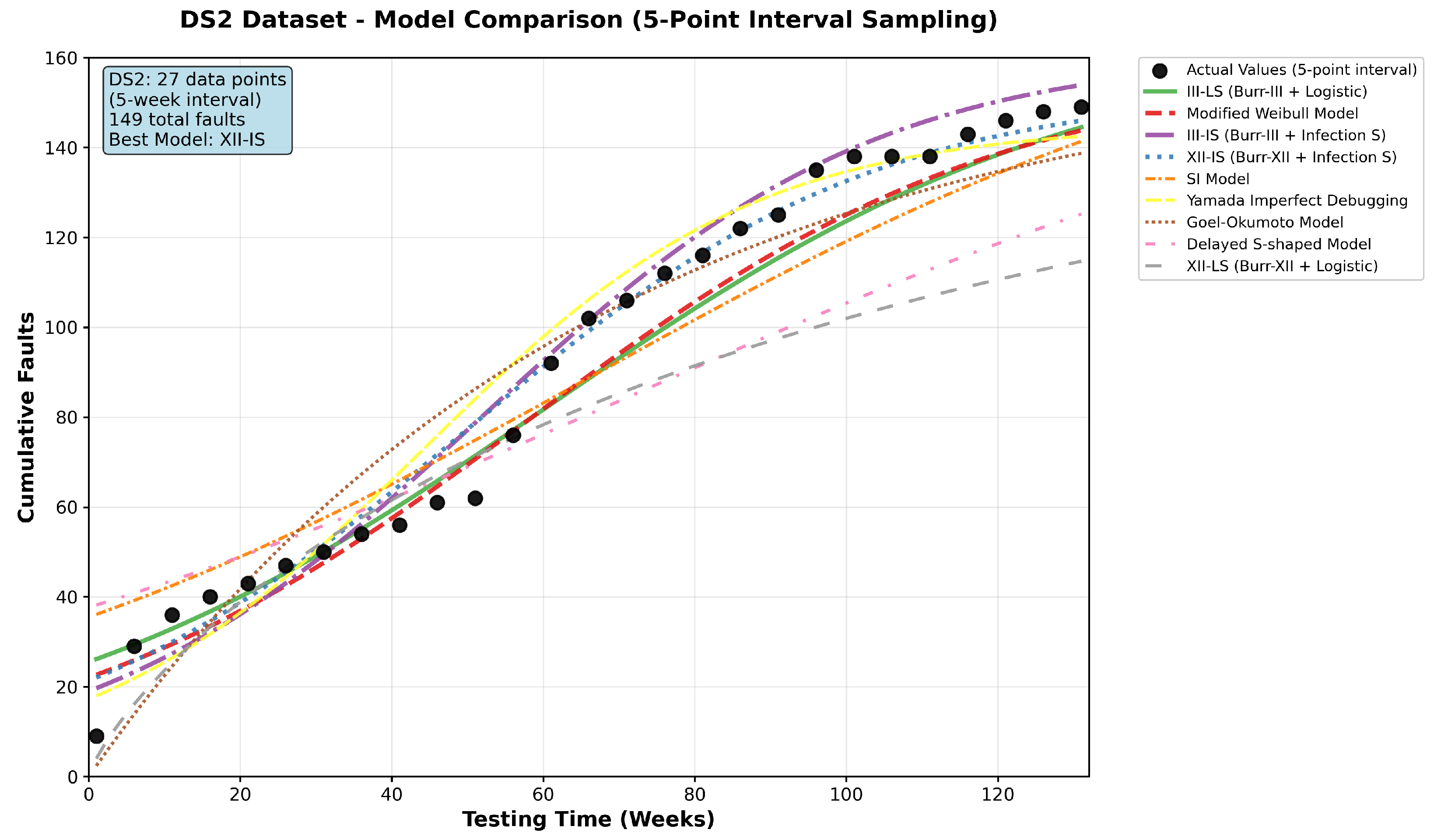
The key findings reveal that S-shaped TEFs, particularly the Infection S-type, are superior for modeling the non-linear consumption of testing effort. Furthermore, the GRU-HMM estimation method proved to be exceptionally robust, especially for complex models and larger datasets, outperforming both LSE and standalone GRU by effectively capturing phase transitions and temporal dependencies. Among the various combinations, the models pairing Burr distributions with the Infection S-shaped TEF (III-is and XII-is) consistently delivered the best performance. For instance, the XII-is model achieved an MSE of 48.9 and an AIC of 481.3 on the DS2 dataset, which is a significant improvement over the best baseline model (MSE = 64.2, AIC = 548.9). This highlights the importance of a synergistic model design and a powerful estimator.

To position our contribution within the broader context, we provide a comparative discussion with emerging deep learning-based approaches. Unlike representative frameworks such as the deep neural network weight learning method by Wu et al. and the SRGM-as-activation model by Kim et al., which primarily rely on the temporal learning capability of networks, our GRU-HMM framework is explicitly designed to capture the discrete phase transitions inherent in software testing efforts. This fundamental architectural difference—the synergistic combination of GRU for temporal dynamics and HMM for latent phase inference—provides a principled solution to a key challenge in reliability modeling, offering a more structured and interpretable approach that is theoretically better suited for handling non-stationary dynamics.

Practically, the achieved higher prediction accuracy directly translates into more reliable release decisions and optimized testing resource allocation, potentially reducing costly post-release failures. Future work will focus on developing an automated framework for optimal model selection and optimizing the computational efficiency of the GRU-HMM estimator for broader deployment.