Article

Valuation of Defaultable Corporate Bonds Under Regime Switching

1
Department of Business Administration, Fu Jen Catholic University, No. 510, Zhongzheng Rd., Xinzhuang Dist., New Taipei City 242062, Taiwan
2
Department of Business Administration, National Chin-Yi University of Technology, No. 57, Sec. 2, Zhongshan Rd., Taiping Dist., Taichung 411030, Taiwan
*
Author to whom correspondence should be addressed.
Mathematics 2025, 13(22), 3628; https://doi.org/10.3390/math13223628
Submission received: 29 September 2025 / Revised: 6 November 2025 / Accepted: 7 November 2025 / Published: 12 November 2025

Abstract

This study investigates the valuation of defaultable corporate bonds using a two-factor model of Markov-modulated stochastic volatility with double exponential jumps (2FMMSVDEJ). This model captures long- and short-term SV and asymmetrical jumps in the underlying asset value. Concurrently, the firm’s debt dynamics are governed by a Markov-modulated GBM (MMGBM) model to reflect state transitions. A dynamic measure change technique is employed to determine the pricing kernel, and the resulting credit spreads and default probabilities are analyzed.

1. Introduction

With the increasing proliferation of credit derivatives in the financial market, credit risk measurement and risk supervision have become the focus of attention. As bonds with default risk, corporate bonds are traditional financial instruments that bear corporate credit risks. Among them, one necessary step is to appropriately construct a dynamic model that captures the dynamics of a company’s asset values and debt. Then, a fair valuation of defaultable corporate bonds can be provided explicitly or practically. From the theory and practice perspective, the valuation of corporate bonds is a crucial issue in finance [1,2,3,4].
Reviewing previous studies, corporate bond valuation has two main methods: the structural and reduced models. The latter regards the default event as determined by the company exogenous variables, whereas the former is another important default model in addition to the reduced model. Following the methods proposed by [5] and [6], the structural model adopts the concept of call option valuation. The value of shareholders’ equity is taken as the underlying company asset and that of company debt as the exercise price of a European-style call option value. [6] proposed a structural model that uses company structured variables to determine the default time. He believed that at the bond’s maturity date, as long as company assets are insufficient to cover debt, a default will occur. Furthermore, [7] improved the definition of default events in the model of [6] and incorporated stochastic interest rates into defaultable bond valuation. More generally, the pricing of such defaultable derivatives where the payoff is contingent on a stochastic event time involves distinct theoretical frameworks, such as stopped SDEs or intensity-based models, as comprehensively analyzed in [8]. Under the research framework of [6,9] and [10] assumed that the company asset value process is a geometric Brownian motion (GBM). They studied the problem of optimal capital structure when the company asset value is below the liability threshold and has breached the contract. The above structural model assumes that the company asset value is subject to a continuous diffusion. Hence, the theoretical result of bond credit spread is smaller than the actual market situation. [11] embedded a structural model of credit risk inside a dynamic continuous-time consumption-based asset pricing model. However, company stock price has undergone discontinuous jumps because of external instability factors, such as the global financial crisis and currency devaluation, which often results in a substantial decrease in asset value and jumps. [12] found that although the return on financial assets jumps, non-Gaussian properties are also observed. [13] and [14] incorporated the compound Cox process into company asset value dynamics to make up for the previous structural model’s shortcomings and construct a credit spread curve that is more in line with various shapes in reality. [15] incorporated the jumping component into the dynamic process of asset value. They used the time-varying Lévy model to analyze the company capital structure and studied the company endogenous bankruptcy probability. However, in this time-varying Lévy model, only a downward jumping process exists, which cannot describe the upward jumping phenomenon of the company asset value. [16] incorporated the compound Cox process into the KMV equation, depicting the jumping phenomenon caused by rare events. They used financial data to analyze the jumps in the value of the company assets and then estimated the distance and probability of default. The research model assumed that the number of jumps obeys the Poisson distribution, and the random jump amplitude follows the normal distribution. However, the normally distributed jump amplitude could not capture the leptokurtic distribution and fat-tail phenomenon of the actual data return. [17] and [18] confirmed that the double exponential distribution fits the leptokurtic and fat-tail phenomena, which could better meet the actual demand in financial modeling. This Lévy process could simultaneously reflect jumps in the rise and fall of market prices, which is more in line with the actual financial market situation [19]. Considering the memorylessness of the double exponential distribution, [20] pointed out that incorporating a double exponential distribution setting into the jump-diffusion option pricing model will enable analytical solutions to various types of option valuation results. Nevertheless, the analytical solution cannot be obtained using the jump-diffusion model under the normal distribution. Thus, the double exponential jump-diffusion (DEJD) model has an excellent application advantage in financial risk measurement and management.
The state-dependent dynamics allow the model’s volatility to change with economic conditions over time. Thus, Markovian regime-switching models are widely used in finance and econometrics for depicting the changing volatility in asset returns. [21] illustrated that as an essential component of the asset return process, stochastic volatility should be included in the DEJD model. [22] studied the foreign exchange rates of JPY/USD and EUR/USD and provided support for using a Markov-modulated DEJD model for formulations. Their evidence supports the use of Markov-modulated DEJDs for modeling an underlying asset price process, which can improve the accuracy of option pricing. Incorporating interest rate risk is critical for improving the accuracy of option pricing. Hence, [23] presented a semi-closed-form pricing model for barrier options. The underlying asset price follows a mean-reverting and Markovian regime-switching DEJD process, and a mean-reverting square root model modulates the interest rate.
Under the research framework of [17], the DEJD model fails to describe volatility clustering and the long memory phenomenon. Therefore, in this study, the dynamics of company asset value are driven by a two-factor model of Markov-modulated stochastic volatility with double exponential jumps (2FMMSVDEJ). This model is used for depicting long- and short-term stochastic volatility and asymmetrical jumps, extending the structural model proposed by [13] and [14]. Moreover, the dynamics of company debt are governed by a Markov-modulated GBM (MMGBM) model, which captures the character of state transition through time. More specifically, the states of that Markov chain represent an economy’s hidden states. The Markov-modulated risk caused by regime shifts can hardly be diversified because it is more likely to be regarded as systematic risk. Hence, the securities market is incomplete. [24] used the Esscher transform developed by [25] for option pricing and justified its use with the minimal-entropy, risk-neutral martingale measure. In an incomplete market with jumps and stochastic volatility, the choice of an appropriate martingale measure is itself a significant academic issue. [26] thoroughly compared the properties and differences in various equivalent martingale measures (such as the Esscher transform, the minimal entropy martingale measure (MEMM), and the minimal martingale measure) in complex stochastic volatility models, like the Barndorff-Nielsen and Shephard (BNS) model. Within the Markov setting, an increasing number of studies ([27,28,29,30,31,32,33]) used measure changes in the Esscher transforms of underlying asset price dynamics to determine pricing kernels. We are interested in discovering a formula for solving such a bond pricing problem in our model framework. This study extends the Esscher transform technique to price the defaultable corporate bonds.
Regarding asset pricing, while existing literature has explored stochastic volatility or jumps, this study establishes a 2FMMSVDEJ model. This model simultaneously captures long-term structural volatility driven by regime shifts and short-term volatility driven by a stochastic process, combined with asymmetrical double exponential jumps. Second, regarding the liability structure, this study introduces a significant innovation: instead of assuming static debt, we model the firm’s debt itself as a MMGBM. This allows the firm’s asset and debt dynamics to be jointly driven by the same hidden economic states (e.g., boom or recession). This provides a more realistic and practical foundation for credit risk assessment. For instance, in a recession state, a firm may face simultaneously decreasing asset values and increasing debt volatility, a correlated effect that traditional models may underestimate. Finally, in the resulting incomplete market, we successfully extend the Esscher transform technique to determine a consistent pricing kernel, thereby deriving semi-analytical solutions for defaultable corporate bonds. Differently from the model setting of [14,19], and [32], we simultaneously incorporate the long- and short-term stochastic volatility and asymmetrical jumps into company asset value and consider the regime-switching risks of the company debt. This overcomes the disadvantages of previous works and contributes to the corporate bond pricing literature.
The remainder of this study is organized as follows. Section 2 provides the dynamic model. Section 3 presents the change in measures. Section 4 illustrates the fair valuation of defaultable corporate bonds. Section 5 demonstrates the numerical examples. Finally, Section 6 concludes the study.

2. Model Framework

Let Ω , F , P   be a complete filtered probability space P on which all subsequent stochastic processes (the Markov chain ξ ( t ) , the Brownian motion W ( t ) , and the Cox process N ( t ) ). We define a continuous-time, finite-state Markov chain ξ ( t ) on Ω , F , P   with state space = 1 , 2 , , I for all t 0 , T . The states of ξ ( t ) can be interpreted as an economy’s hidden states. Without any loss of generality, we can take state space for ξ ( t ) to be a finite set of unit vectors e 1 , e 2 , , e I with e j = 0 , , 1 , , 0 I . [24,34] provided a semi-martingale representation for ξ ( t ) as follows:
d ξ ( t ) = Π ξ ( t ) d t + d M ( t ) ,
where M ( t ) is an I -valued martingale concerning the natural filtration generated by ξ ( t ) under P . Let Π = π i , j i , j = 1 , 2 , , I denote the generator, or rate matrix, of ξ ( t ) under P , where π i , j is the transition intensity of ξ ( t ) from state e i to e j .
Let V ( t ) represent the company asset value at time t . We further establish the 2FMMSVDEJ model to depict the dynamic behavior of long- and short-term stochastic volatility and asymmetrical jumps in company asset value, which is given by the following:
d V ( t ) V ( t ) = α ( t ) λ ( t ) κ d t + σ l ( t ) d W 1 ( t ) + U ( t ) d W 2 ( t ) + exp ( Z ( t ) ) 1 d N ( t ) , d U ( t ) U ( t ) = δ d t + ν d W u ( t ) ,
for all t 0 , T . The first stochastic volatility, σ l ( t ) , changes over time according to the state transition of ξ ( t ) , which is used to capture occasional jumps in long-term fluctuations. The second stochastic volatility, U ( t ) , of the company asset value follows a log-normal diffusion, which is used to describe the frequent random perturbation behavior of short-term fluctuations with constant rate of drift and δ as well as the volatility parameters v . In addition, V ( t ) and U ( t ) represent the value of the function immediately before time t (càdlàg processes). The appreciation rate, α ( t ) , the first stochastic volatility, σ l ( t ) , of the company asset value, and the stochastic arrival intensity, λ ( t ) , of the Cox process, N ( t ) , ξ ( t ) as follows:
α ( t ) = α , ξ ( t ) ,   α = α ( 1 ) , α ( 2 ) , , α ( I ) I ,
σ l ( t ) = σ l , ξ ( t ) ,   σ l = σ l ( 1 ) , σ l ( 2 ) , , σ l ( I ) ( 0 , ) I ,
and
λ ( t ) = λ , ξ ( t ) ,   λ = λ ( 1 ) , λ ( 2 ) , , λ ( I ) 0 , I ,
where , denotes the inner product in I . The correlated Wiener processes of Equation (2) are defined by d W u ( t ) = ρ ( t ) d W 1 ( t ) + 1 ρ 2 ( t ) d W 2 ( t ) for W 1 ( t ) W 2 ( t ) , the instantaneous correlation coefficient at time t is given by ρ ( t ) = ρ , ξ ( t ) , and ρ = ρ ( 1 ) , ρ ( 2 ) , , ρ ( I ) I with 1 < ρ ( j ) < 1 for j = 1 , 2 , , I . In addition, if a jump event occurs at time t , the random variable Z ( t ) controlling the jump amplitude is assumed to be a double exponential distribution with a probability density function given by:
f Z ( y ) = p η 1 exp η 1 y 1 y 0 + ( 1 p ) η 2 exp η 2 y 1 y < 0 ,   η 1 > 1 ,   η 2 > 0 .
where η 1 ( η 1 > 1 ) and η 2 ( η 2 > 0 ) denote the sensitivities of investors to the external bullish and bearish news, respectively. A larger η value indicates that the market is less sensitive to external shocks and the investment response is insufficient. Specifically, η 1 > 1 is required to ensure that E exp Z ( t ) < and E V ( t ) < , indicating that the average upward jump cannot exceed 100%. Furthermore, 1 is an indicator function, and Z ( t ) possesses an exponential random variable φ + with upward jump probability p , mean 1 η 1 , and an exponential random variable φ with downward jump probability ( 1 p ) and mean 1 η 2 . Consequently, the mean percentage jump amplitude of the company asset value is κ = E exp Z ( t ) 1 = p η 1 η 1 1 + ( 1 p ) η 2 η 2 + 1 1 = ϕ Z ( 1 ) 1 . Compared with a normal distribution, a double exponential distribution depicts the leptokurtic feature of company asset value data. In Equation (2), we assume that Z ( t ) and Z ( s ) are independent for t s , and all random shocks W 1 ( t ) , W 2 ( t ) , N ( t ) , ξ ( t ) , and Z ( t ) are mutually independent.
We aim to capture the time-inhomogeneity of company debt according to market state transition. Thus, we establish a MMGBM model with regime-switching risks to describe the state-dependent pure diffusion process of company debt, D ( t ) , under an incomplete market setting, which is given by the following:
d D ( t ) D ( t ) = μ ( t ) d t + σ D ( t ) d W D ( t ) ,
where the appreciation rate, μ ( t ) , and the stochastic volatility, σ D ( t ) , of the company debt are modulated by ξ ( t ) as follows:
μ ( t ) = μ , ξ ( t ) ,   μ = μ ( 1 ) , μ ( 2 ) , , μ ( I ) I ,
and
σ D ( t ) = σ D , ξ ( t ) ,   σ D = σ D ( 1 ) , σ D ( 2 ) , , σ D ( I ) ( 0 , ) I ,
and W D ( t ) is a Brownian motion under P . Furthermore, the risk-free instantaneous interest rates are defined by r ( t ) as follows:
r ( t ) = r , ξ ( t ) ,   r = r ( 1 ) , r ( 2 ) , , r ( I ) 0 , I ,

3. Esscher Transform for 2FMMSVDEJ–MMGBM Dynamics

In an incomplete market setting, we employ the Esscher transform method ([24] and [27,28,29,30,31,32,33,34]) for 2FMMSVDEJ–MMGBM dynamics to determine an equivalent martingale measure. For all t 0 , T , we decompose the dynamics of 2FMMSVDEJ logarithmic return R ( t ) = log V ( t ) / V ( 0 ) = C ( t ) + J ( t ) into a continuous diffusion component C ( t ) = 0 t α ( s ) λ ( s ) κ 1 2 σ l 2 ( s ) 1 2 U ( s ) d s + 0 t σ l ( s ) d W 1 ( s ) + 0 t U ( s ) d W 2 ( s ) and a jump component J ( t ) = 0 t Z ( s ) d N ( s ) . Here, let F t R t 0 , T and F t ξ t 0 , T be the right-continuous, P -complete, and natural filtrations generated by stochastic processes R ( t ) t 0 , T and ξ ( t ) t 0 , T , respectively. For each t 0 , T , we define F t = F t R F t ξ as the enlarged σ -algebra. We assume that trading occurs continuously in time over interval 0 , T and uncertainty is described by a filtered probability space, Ω , F , P   , F t t 0 , T . In this case, the Radon-Nikodym derivative of the Markov-modulated Esscher transform is provided as follows:
η θ ( t ) = d Q θ d P F t = exp 0 t θ ( s ) d C ( s ) + 0 t d J ( s ) E exp 0 t θ ( s ) d C ( s ) + 0 t d J ( s ) F t ξ ,
where θ ( t ) = θ , ξ ( t ) and θ = θ ( 1 ) , θ ( 2 ) , , θ ( I ) I , in which θ ( t ) is the Markov-modulated Esscher parameter of C ( t ) . Here, Q θ represents the Esscher measure and the Markov-modulated Esscher transform density process, η θ ( t ) , is an exponential F t -martingale.
To value defaultable corporate bonds fairly, we apply the insights of [35] and [36] to characterize the dynamic conditions of company asset value and debt such that an equivalent martingale measure exists. The risk-neutral Esscher measure can be selected as Q θ such that discounted asset price dynamics are Q θ -martingales. This case is obtained by determining the Markov-modulated Esscher parameter θ ( t ) as the solution for the martingale condition E θ exp 0 t r ( s ) d s V ( t ) F 0 = V ( 0 ) . We assume that the Markov-modulated Esscher transform is defined by Equation (11) from the mutual independence of random shocks. According to the (A3), the martingale condition under the risk-neutral probability measure Q θ is given as follows:
α ( t ) + λ ( t ) ϕ Z ( 2 ) ϕ Z ( 1 ) 1 2 σ l ( t ) 2 1 2 U ( t ) 1 2 θ ( t ) 2 + 1 2 σ l ( t ) + U ( t ) + θ ( t ) 2 = 0 ,
where 0 s u t T ¯ . denotes the norm in I and the moment-generating function Z ( t ) is ϕ Z ( u ) = E exp u Z ( t ) = p η 1 η 1 u + ( 1 p ) η 2 η 2 + u , η 1 > u , η 2 > u . Appendix A provides detailed proof. Notably, the compensated Cox process can be denoted by E θ t = 1 N θ ( t ) exp Z θ ( t ) 1 = λ θ ( t ) ϕ Z θ ( 1 ) 1 t = λ ( t ) κ t under the risk-neutral probability measure Q θ . The jump amplitude variable, Z θ ( t ) , is a double exponential distribution with parameters η 1 , η 2 , and p . The Cox process, N θ ( t ) , with stochastic arrival intensity, is given by λ ( t ) .
Therefore, the dynamics of the company asset value under Q θ is given as follows:
d V ( t ) V ( t ) = r ( t ) λ ( t ) κ d t + σ V ( t ) d W V θ ( t ) + exp ( Z θ ( t ) ) 1 d N θ ( t ) ,
where σ V ( t ) d W V θ ( t ) = σ l ( t ) d W 1 θ ( t ) + U ( t ) d W 2 θ ( t ) with σ V ( t ) = σ l 2 ( t ) + U ( t ) . Furthermore, using the random Esscher transform, the dynamics of MMGBM company debts under Q θ is given as follows [31]:
d D ( t ) D ( t ) = r ( t ) d t + σ D ( t ) d W D θ ( t ) ,
Specifically, the correlated Wiener processes of Equations (13) and (14) are defined by d W D θ ( t ) = ρ V D ( t ) d W 1 θ ( t ) + 1 ρ V D 2 ( t ) d W 2 θ ( t ) for W 1 θ ( t ) W 2 θ ( t ) . The instantaneous correlation coefficient at time t is given by ρ V D ( t ) = ρ V D , ξ ( t ) and ρ V D = ρ V D ( 1 ) , ρ V D ( 2 ) , , ρ V D ( I ) I with 1 < ρ V D ( j ) < 1 for j = 1 , 2 , , I . In Equations (13) and (14), all randomness is assumed to be mutually independent.

4. Valuation of Defaultable Corporate Bonds

In this subsection, we derive the closed-form solution for defaultable corporate bonds within the 2FMMSVDEJ–MMGBM framework under a simplified condition. In the general circumstance, the default probability of the corporate bonds was obtained, and the term structure of the credit spreads was discussed. The model parameters can be explicitly expressed in terms of the occupation times of the state of Markov chain ξ ( t ) . Let O j t , T denote the occupation time of ξ ( t ) in state j ( j = 1 , 2 , , I ) over time duration t , T with t < T . We define:
t T r ( u ) d u = j = 1 I r ( j ) O j ( t , T ) ,
t T σ l 2 ( u ) d u = j = 1 I σ l 2 ( j ) O j ( t , T ) ,   t T U ( u ) d u ,
t T σ D 2 ( u ) d u = j = 1 I σ D 2 ( j ) O j ( t , T ) ,
and
λ θ ( t , T ) = t T λ ( u ) d u = j = 1 I λ ( j ) O j ( t , T ) .

4.1. Simplified Condition: The Corporate Bond May Default Only at Maturity T

In financial markets, we assume the company repays its debt in full (i.e., the bondholder receives a face value of one currency unit) if X ( T ) = V ( T ) / D ( T ) 1 at maturity T . Moreover, a default occurs (i.e., the bondholder will get a face value of 1 ω ( X ( T ) ) currency unit) if X ( T ) = V ( T ) / D ( T ) < 1 at maturity T . Let ω ( X ) denote the bondholder’s loss rate if the company defaults, which is a non-increasing function for X . 1 ω ( X ) represents the recovery of a bond. Here, we set ω ( X ) = ω 0 ω 1 X , where ω 0 and ω 1 are non-negative constants. Thus, the price of a zero coupon bond (ZCB) at time t paying one currency unit at maturity T under Q θ is given as follows:
P t , T ; X F t = E θ exp t T r ( u ) d u 1 X ( T ) 1 + exp t T r ( u ) d u 1 ω ( X ( T ) ) 1 X ( T ) < 1 F t .
In a risk-neutral environment, the no-arbitrage price of ZCB at time t paying one currency unit at maturity T is achieved as follows:
P O j ; X F t = exp t T r ( u ) d u ω 0 exp t T r ( u ) d u 1 ϒ t T σ D 2 ( u ) ρ V D ( u ) σ V ( u ) σ D ( u ) 1 2 σ 2 ( u ) d u κ t T λ ( u ) d u , t T σ 2 ( u ) d u , t T λ ( u ) d u , p , η 1 , η 2 ; ln X ( t ) + ω 1 X ( t ) 1 ϒ t T σ D 2 ( u ) ρ V D ( u ) σ V ( u ) σ D ( u ) + 1 2 σ 2 ( u ) d u κ t T λ ( u ) d u , t T σ 2 ( u ) d u , t T λ ( u ) d u , p , η 1 , η 2 ; ln X ( t ) ,
where ϒ ( ) denotes the cumulative distribution function of a double exponential random variable ([17] and [18]), and
t T λ ( u ) d u = ϕ Z ( 1 ) t T λ ( u ) d u ,
p = p η 1 ϕ Z ( 1 ) η 1 1 ,
η 1 = η 1 1 ,
and
η 2 = η 2 + 1 .
Appendix B provides detailed proof. Therefore, the pricing formula of a defaultable ZCB, in terms of the occupation times, obeys the following semi-analytic form:
P t , T ; X = [ t , T ] I j P O j ; X F t Ψ O j d O j ,   j = 1 , 2 , , I ,
where Ψ O j = Ψ O 1 , O 2 , , O I denotes the joint probability distribution density for the occupation time. We write O ( t , T ) = O 1 t , T , O 2 t , T , , O I t , T for the vector of occupation times. Notably, Ψ O 1 , O 2 , , O I can be completely determined by the following:
E exp i ε , O t , T F t ξ = ξ ( t ) exp Π + i D T t , 1 ,
where i = 1 , 1 = 1 , 1 , , 1 I , and matrix D denotes a diagonal matrix consisting of the elements in vector ε = ε 1 , ε 2 , , ε I as diagonal, such as in [24].

4.2. Generalized Condition: The Bond May Default at or Before Maturity T

Generally, the first passage time of a generalized jump-diffusion process X ( t ) to a flat boundary: τ : = inf t 0 , X ( t ) = V ( t ) / D ( t ) 1 should be defined to price defaultable ZCBs for 2FMMSVDEJ–MMGBM dynamics. We assume that if the company defaults before maturity T , the bondholder will obtain a face value of 1 ω ( X ( τ ) ) currency unit at maturity T , in which τ denotes the first passage time of V ( t ) for D ( t ) or the time of V ( t ) is less than that of D ( t ) . Hence, the price of ZCB at time t paying one currency unit at maturity T under Q θ is given as follows:
P t , T ; X F t = E θ exp t T r ( u ) d u 1 τ > T + exp t T r ( u ) d u 1 ω ( X ( τ ) ) 1 τ T F t = exp t T r ( u ) d u exp t T r ( u ) d u E θ ω ( X ( τ ) ) 1 τ T F t .
According to a company’s default time, denoted by τ , the default probability of a ZCB is provided as follows:
Q θ τ T = Q θ inf t u T X ( u ) 1 = Q θ inf t u T Y ( u ) ln X ( t ) ,
However, obtaining the explicit solution of Equation (28) for generalized jump-diffusion processes will be very difficult. [37] used the memoryless property of a double exponential distribution to derive the explicit solution of the Laplace transform regarding the distribution of the first passage times of a DEJD model. Consequently, under the 2FMMSVDEJ–MMGBM model of this study, the default probability of a corporate bond can be obtained by calculating the Laplace transform of Q θ τ T as follows:
0 exp a T Q θ τ T d T = 1 a 0 exp a T d Q θ τ T = 1 a E θ exp a τ ,
In line with Equation (A6) and for any a 0 , , let β 3 , a and β 4 , a be the only two negative roots for the following equation:
G ( x ) = x σ D 2 ( s ) ρ V D ( s ) σ V ( s ) σ D ( s ) λ ( s ) κ 1 2 σ 2 ( s ) + 1 2 x 2 σ 2 ( s ) + λ ( s ) p η 1 η 1 x + ( 1 p ) η 2 η 2 + x 1 = a ,   0 < β 3 , a < η 2 < β 4 , a < ,
and by using the result of the first passage times within a DEJD model of [37], we further derive the following:
E θ exp a τ = η 2 β 3 , a η 2 β 4 , a β 4 , a β 3 , a exp ln X ( t ) β 3 , a + β 4 , a η 2 η 2 β 3 , a β 4 , a β 3 , a exp ln X ( t ) β 4 , a
In Equation (30), G ( ) is defined as the moment-generating function of Y ( t ) with the equation: E θ exp Θ Y ( t ) = exp G ( Θ ) t . In practice, the one-dimensional Laplace transform inversion algorithm of Gaver–Stehfest can be used to obtain the numerical solution of the aforementioned probability of default, as described and implemented by [18,37].

5. Numerical Illustrations

For the numerical illustrations, we apply the risk-neutral dynamics of the asset value and debt according to Equations (13) and (14), respectively. Then, we use the Monte Carlo simulation under the Markov chain ξ ( t ) with two economic states, videlicet, “boom” and “recession” states for the economy. The two-state transition probability of Markov chain is defined as follows:
p 11 p 12 p 21 p 22 = 0.95 0.05 0.15 0.85 .
The initial value of the asset, debt, and Markov chain state is set to be V ( 0 ) = 50 , D ( 0 ) = 25 , and ξ ( 0 ) = [ 1 , 0 ] , respectively. [14] noted that the loss rate parameters ω 1 are set to be 1.4 and 1, respectively. Table 1 presents the remaining model parameters for numerical analyses. Furthermore, we simulate 50 thousand times with a discretization interval of 1/365 setting to derive defaultable bond prices.

5.1. Generalized Condition Analytics

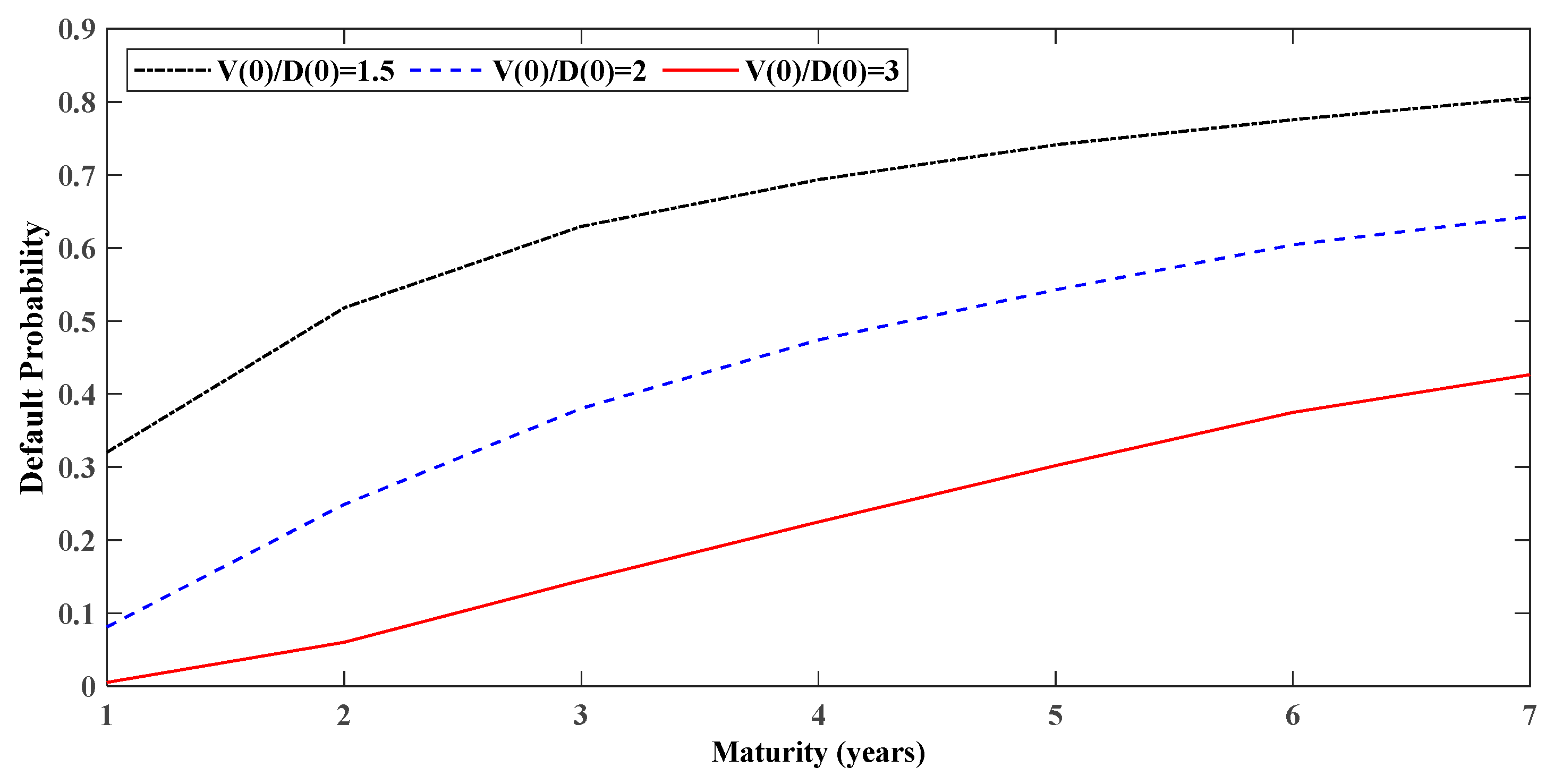
The simplified condition is the special case of the generalized condition. Therefore, the analyses of this study will focus more on generalized cases. According to the generalized condition, we investigated the impact of the current X ( 0 ) = V ( 0 ) / D ( 0 ) on credit spread and the default probability. We found that the larger X ( 0 ) corresponds to the smaller credit spread and smaller default probability from Figure 1 and Figure 2. Moreover, the larger X ( 0 ) means that the leverage ratio for the company is much smaller, which is much more secure for the bondholder. Hence, the credit spread is much smaller with larger X ( 0 ) . In addition, the larger X ( 0 ) implies that the company asset consists of less part of the liability. Thus, the ability of the company to pay is very good. Furthermore, the credit spread for the lower X ( 0 ) , such as X ( 0 ) = 1.5 , decreases with the time to maturity, whereas the default probability increases.
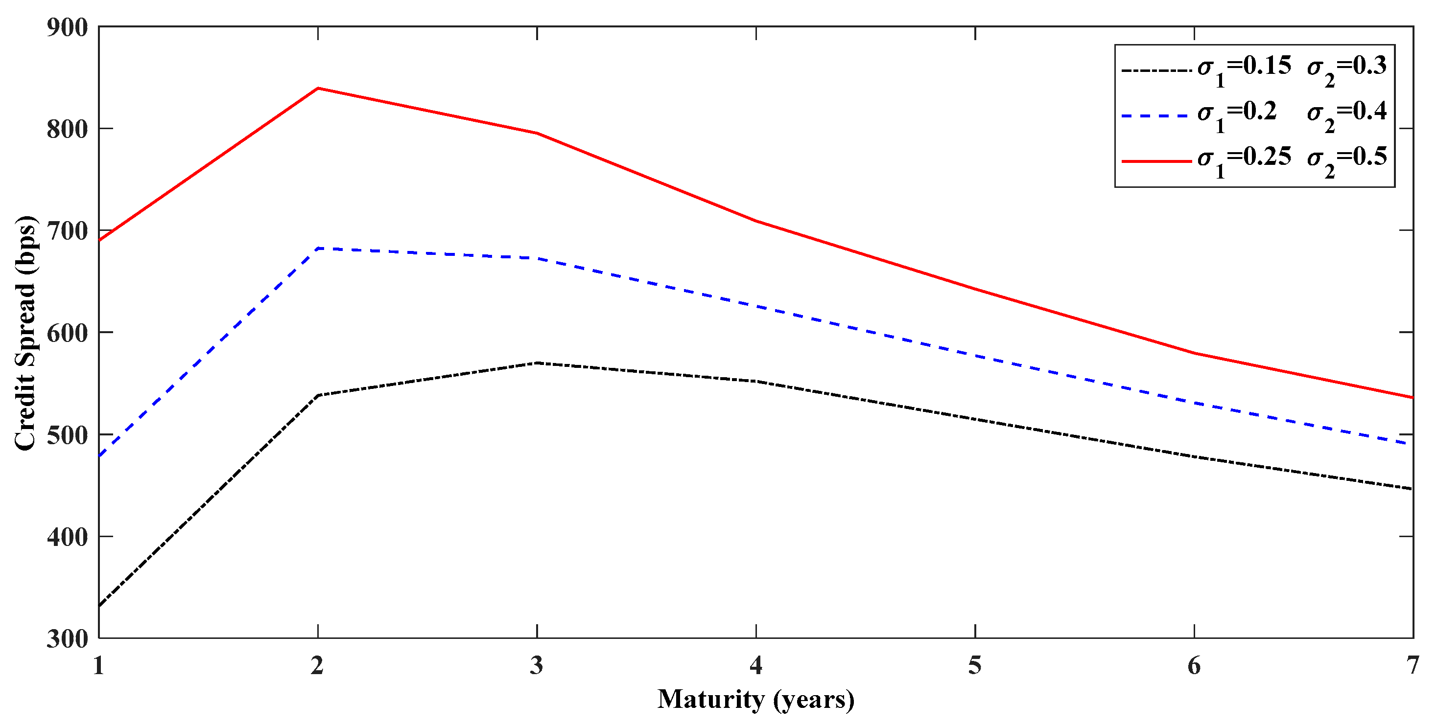
Figure 3 shows that the credit spread will enlarge with the increase in the long-term volatility. Then, with the increase in time to maturity, the gap among these three long-term volatilities decreases. Figure 4 depicts that the default probability will increase with long-term volatility.
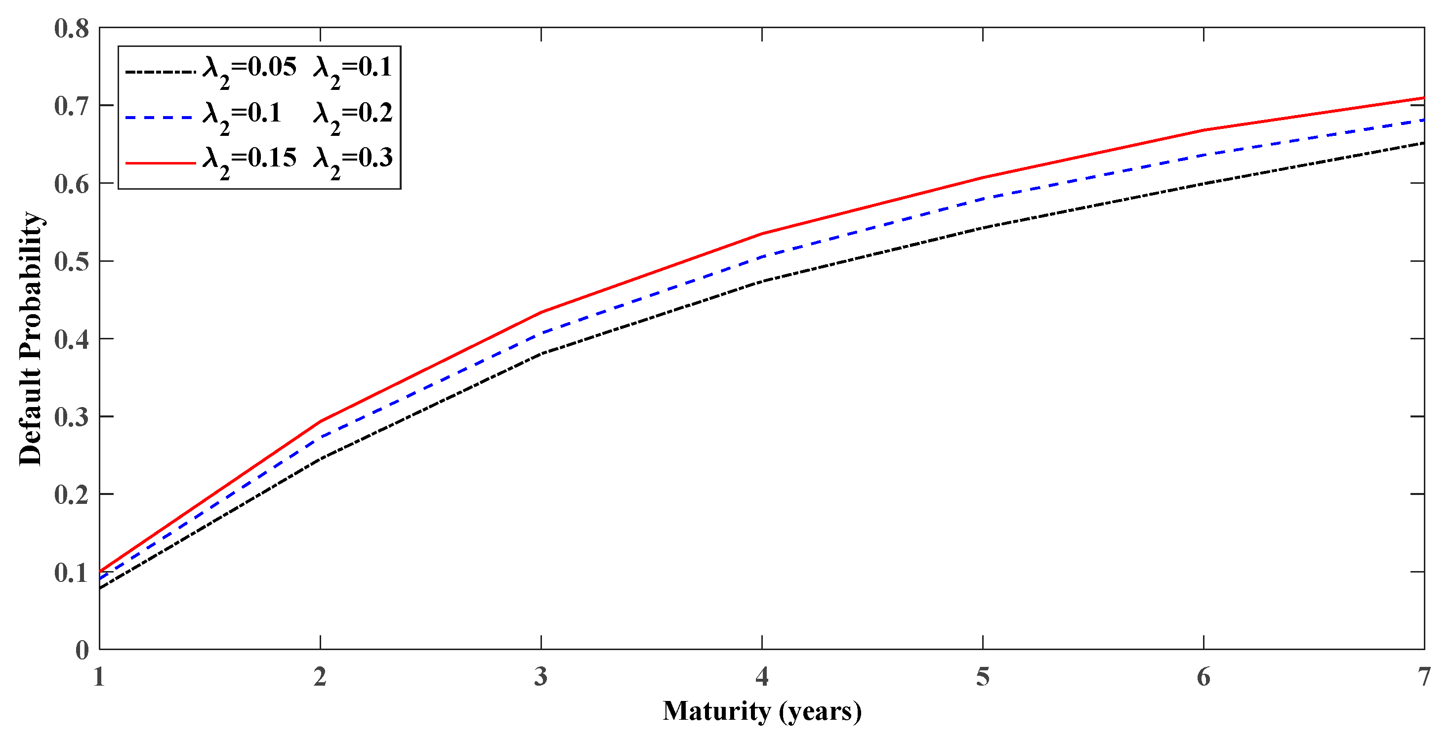
Figure 5 illustrates that the increase in occurrences of event frequency will increase the credit spread to investigate the impact of the “boom” and “recession” states frequency (jump frequency) on credit spread. The reason is that increasing the jump frequency will also increase asset volatility. Furthermore, the default probability will increase with the increase in jump frequency, as shown in Figure 6.
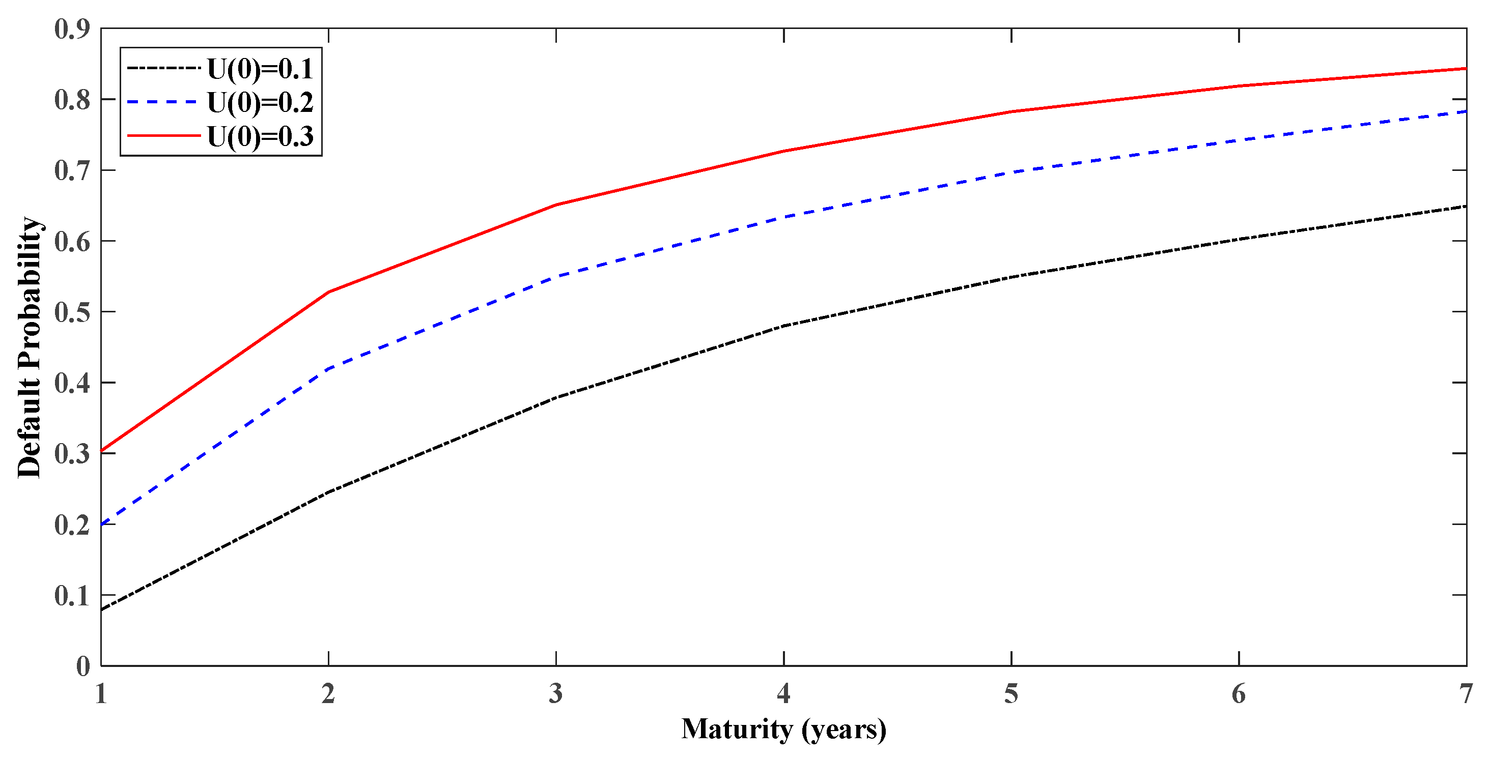
Comparing Figure 3 and Figure 7, we find that the initial short-term volatility has more impact on increasing the credit spread than the long-term volatility. This case may be because of the sudden impact of the short-term stochastic volatility, making asset prices suddenly more volatile, pushing asset prices below the debt. The default probability will also increase with the initial short-term stochastic volatility, as shown in Figure 8.

5.2. Comparison of the Simplified and Generalized Conditions

We compare the credit spread and default probability under these two conditions with the scenario of different asset and debt initial ratios. The upper and lower panels of Figure 9 are for the simplified (default only at maturity) and generalized conditions, respectively. We found that the default probability for the generalized case is larger than the simplified one. This result is intuitive because the generalized one does not set any time restriction to default. Hence, as the asset value is below the debt, the default event will be triggered. However, for the simplified condition, a restriction of time to default exists. Therefore, although the asset value is below the debt before maturity, the default event is still not triggered unless the asset value is below the debt until maturity. The credit spread is not very intuitive. We found that the generalized condition is much larger for the short maturity than the simplified one under the lower V ( 0 ) / D ( 0 ) . However, for the long maturity, the credit spread under the generalized condition is much smaller than the simplified one. The case of higher default probability with lower credit spread may be because the definition of default did not consider the time to default.

6. Conclusions

We evaluated the defaultable corporate bond prices by providing a 2FMMSVDEJ–MMGBM model. Under the no-arbitrage framework of the stochastic interest rates, we employed a 2FMMSVDEJ–MMGBM model for company asset value and debt, modeling from a physical to a risk-neutral measure. Compared with most existing Markov-modulated models, our model’s main advantage is that we incorporated long- and short-term stochastic volatilities, double exponential jumps, jump intensity switching, and regime-switching interest rates into the asset price dynamics. Under an incomplete market setting, we employed the Markov-modulated Esscher transform to identify a martingale measure for pricing defaultable corporate bonds. This study concludes that the stochastic volatilities (of company asset values and debts) and jump frequencies significantly influence bond prices according to the pricing results. Furthermore, the default probability and credit spread of corporate bonds were discussed for the generalized condition. As a result, this study contributes to the literature about the time-inhomogeneity and asymmetrical jump impacts on defaultable corporate bond prices. In addition, our model jointly models asset and debt dynamics providing direct relevance for risk management. This framework allows for more practical and realistic assessment by quantifying how default probabilities and credit spreads change significantly as the economy transitions between “boom” and “recession” states.

Author Contributions

Y.-M.L.: conceptualization, methodology, software, writing—original draft, writing—review and editing. J.-H.C.: methodology, software, writing—original draft. All authors have read and agreed to the published version of the manuscript.

Funding

Y.-M.L. is grateful to the Taiwan Ministry of Science and Technology for support through Project No.: MOST109-2410-H-030-019-MY2 and the National Science and Technology Council of Taiwan for support through Project No.: NSTC114-2410-H-030-036.

Data Availability Statement

No new data were created or analyzed in this study.

Acknowledgments

The authors thank the anonymous referees for their helpful comments and suggestions.

Conflicts of Interest

The authors declare no conflicts of interest.

Appendix A. Martingale Condition

Proof. 
Let E θ denote the mathematical expectation operator concerning the risk-neutral Esscher measure as Q θ equivalent to P . Applying Equation (11), we obtain:
V ( s ) = E θ exp s t r ( u ) d u V ( t ) F s = E d Q θ d P V ( t ) exp s t r ( u ) d u F s ,
for 0 s u t T ¯ . According to Equation (A1), by applying Fubini’s theorem and through the moment-generating function, we further have:
E exp s t r ( u ) d u + s t σ l ( u ) + U ( u ) + θ ( u ) d W θ ( u ) = exp 1 2 s t σ l ( u ) 2 d u + 1 2 s t U ( u ) d u + 1 2 s t θ ( u ) 2 d u s t α ( u ) d u exp s t λ ( u ) ϕ Z ( 1 + 1 ) ϕ Z ( 1 ) d u .
From the mutual independence of random shocks, the martingale condition E θ exp s t r ( u ) d u V ( t ) F s = V ( s ) holds if and only if θ ( t ) satisfies:
exp 1 2 s t σ l ( u ) + U ( u ) + θ ( u ) 2 d u = exp 1 2 s t σ l ( u ) 2 d u + 1 2 s t U ( u ) d u + 1 2 s t θ ( u ) 2 d u s t α ( u ) d u exp s t λ ( u ) ϕ Z ( 1 + 1 ) ϕ Z ( 1 ) d u
Therefore, we can define the martingale condition for company asset values under Q θ using Equation (12). □

Appendix B. Derivation of the Defaultable Corporate Bond Pricing Formula

Proof. 
We consider the no-arbitrage valuation of a defaultable corporate bond. Let P t , T ; X represent the value of ZCB at time t paying one currency unit at maturity T. We choose the money market account at time t, denoted by B ( t ) = exp 0 t r ( s ) d s , as the numeraire asset to perform a measure change from measure P to risk-neutral probability measure Q θ to facilitate pricing defaultable corporate bonds in a risk-neutral environment. According to Equation (19), the discounted price process of a defaultable corporate bond under Q θ can be expressed as follows:
P t , T ; X F t = exp t T r ( u ) d u exp t T r ( u ) d u E θ ω ( X ( T ) ) 1 X ( T ) < 1 F t = exp t T r ( u ) d u ω 0 exp t T r ( u ) d u E θ 1 X ( T ) < 1 F t + ω 1 exp t T r ( u ) d u E θ X ( T ) 1 X ( T ) < 1 F t ,
and by applying Ito’s formula for Equations (13) and (14), we obtain the following:
d X ( t ) X ( t ) = σ D 2 ( t ) ρ V D ( t ) σ V ( t ) σ D ( t ) λ ( t ) κ d t + σ ( t ) d W θ ( t ) + exp ( Z θ ( t ) ) 1 d N θ ( t ) ,
where σ ( t ) d W θ ( t ) = σ V ( t ) d W V θ ( t ) σ D ( t ) d W D θ ( t ) with the Markov-modulated standard deviation σ ( t ) = σ V 2 ( t ) 2 ρ V D ( t ) σ V ( t ) σ D ( t ) + σ D 2 ( t ) . Therefore, the stochastic process Y ( t ) = ln X ( t ) / X ( 0 ) satisfies:
Y ( t ) = 0 t σ D 2 ( s ) ρ V D ( s ) σ V ( s ) σ D ( s ) λ ( s ) κ 1 2 σ 2 ( s ) d s + 0 t σ ( s ) d W θ ( s ) + 0 t Z θ ( s ) d N θ ( s ) ,
First, we can calculate the following mathematical expectation:
E θ 1 X ( T ) < 1 F t = Q θ X ( T ) < 1 = Q θ Y ( T ) < ln X ( t ) = 1 Q θ Y ( T ) ln X ( t ) = 1 ϒ t T σ D 2 ( u ) ρ V D ( u ) σ V ( u ) σ D ( u ) 1 2 σ 2 ( u ) d u κ t T λ ( u ) d u , t T σ 2 ( u ) d u , t T λ ( u ) d u , p , η 1 , η 2 ; ln X ( t ) , ( T t ) ,
Specifically, we can price a defaultable ZCB by inverting a one-dimensional Laplace transform for the probability distribution in Equation (A7) as in [37] (based on the Gaver–Stehfest algorithm). Analogous calculations can be implemented for the second mathematical expectation in Equation (A4).
Next, to calculate E θ X ( T ) 1 X ( T ) < 1 F t , we construct a new forward martingale measure, Q , associated with numeraire X ( t ) and the jump amplitude. Z ( t ) t 0 , T are double exponential distribution random variables with updating parameters η 1 = η 1 1 , η 2 = η 2 + 1 , and p = p η 1 ϕ Z ( 1 ) η 1 1 . N ( t ) has an updating stochastic arrival intensity given by λ ( t ) = λ ( t ) ϕ Z ( 1 ) for the Cox process and W ( t ) = W θ ( t ) 0 t σ ( s ) d s for the Wiener process. Therefore, the dynamics of Y ( t ) under Q are given as follows:
Y ( t ) = 0 t σ D 2 ( s ) ρ V D ( s ) σ V ( s ) σ D ( s ) λ ( s ) κ + 1 2 σ 2 ( s ) d s + 0 t σ ( s ) d W ( s ) + 0 t Z ( s ) d N ( s ) ,
We can further derive the defaultable corporate bond pricing formula, which is provided by Equation (20), using Equation (A8) to solve the second mathematical expectation in Equation (A4) and combining it with the result of Equation (A7). □

References

  1. Gebhardt, W.R.; Hvidkjaer, S.; Swaminathan, B. The cross-section of expected corporate bond returns: Betas or characteristics? J. Financ. Econ. 2005, 75, 85–114. [Google Scholar] [CrossRef]
  2. van Binsbergen, J.H.; Diamond, W.F.; Grotteria, M. Risk-free interest rates. J. Financ. Econ. 2022, 143, 1–29. [Google Scholar] [CrossRef]
  3. Dickerson, A.; Mueller, P.; Robotti, C. Priced risk in corporate bonds. J. Financ. Econ. 2023, 150, 103707. [Google Scholar] [CrossRef]
  4. van Binsbergen, J.H.; Nozawa, Y.; Schwert, M. Duration-based valuation of corporate bonds. Rev. Financ. Stud. 2025, 38, 158–191. [Google Scholar] [CrossRef]
  5. Black, F.; Scholes, M. The pricing of options and corporate liabilities. J. Political Econ. 1973, 81, 637–654. [Google Scholar] [CrossRef]
  6. Merton, R.C. On the pricing of corporate debt: The risk structure of interest rates. J. Financ. 1974, 29, 449–470. [Google Scholar]
  7. Longstaff, F.; Schwartz, E.S. A simple approach to valuing risky fixed and floating rate debt. J. Financ. 1995, 50, 789–819. [Google Scholar] [CrossRef]
  8. Zaevski, T.S.; Kounchev, O.; Savov, M. Two frameworks for pricing defaultable derivatives. Chaos Solitons Fractals 2019, 123, 309–319. [Google Scholar] [CrossRef]
  9. Goldstein, R.; Ju, N.; Leland, H. An EBIT-based model of dynamic capital structure. J. Bus. 2001, 74, 483–512. [Google Scholar] [CrossRef]
  10. Bharath, D.T.; Shumway, T. Forecasting default with the Merton distance to default model. Rev. Financ. Stud. 2008, 21, 1339–1369. [Google Scholar] [CrossRef]
  11. Bhamra, H.S.; Kuehn, L.-A.; Strebulaev, I.A. The levered equity risk premium and credit spreads: A unified framework. Rev. Financ. Stud. 2010, 23, 645–703. [Google Scholar] [CrossRef]
  12. Charles, C.; Chen, L.J.; Fuh, C.D. The pricing of risk and sentiment: A study of executive stock options. Financ. Manag. 2013, 42, 79–99. [Google Scholar]
  13. Zhou, C.S. A Jump-Diffusion Approach to Modeling Credit Risk and Valuing Defaultable Securities. 1997. Available online: https://ssrn.com/abstract=39800 (accessed on 11 June 2025).
  14. Zhou, C.S. The term structure of credit spreads with jump risk. J. Bank. Financ. 2001, 25, 2015–2040. [Google Scholar] [CrossRef]
  15. Hilberink, B.; Rogers, C. Optimal capital structure and endogenous default. Financ. Stoch. 2002, 6, 237–263. [Google Scholar] [CrossRef]
  16. Huang, R.; Tang, Q.M. Does default risk of the listed company increase since the global financial crisis: Analysis based on the jump changes in Chinese company’s asset value. Manag. Sci. Eng. 2012, 6, 142–148. [Google Scholar]
  17. Kou, S.G. A jump-diffusion model for option pricing. Manag. Sci. 2002, 48, 1086–1101. [Google Scholar] [CrossRef]
  18. Kou, S.G.; Wang, H. Option pricing under a double exponential jump-diffusion model. Manag. Sci. 2004, 50, 1178–1192. [Google Scholar] [CrossRef]
  19. Chen, N.; Kou, S.G. Credit spreads, optimal capital structure, and implied volatility with endogenous default and jump risk. Math. Financ. 2009, 19, 343–378. [Google Scholar] [CrossRef]
  20. Fuh, C.D.; Luo, S.F.; Yen, J.F. Pricing discrete path-dependent options under a double exponential jump diffusion model. J. Bank. Financ. 2013, 37, 2702–2713. [Google Scholar] [CrossRef]
  21. Eraker, B.; Johannes, M.; Polson, N. The impact of jumps in volatility and returns. J. Financ. 2003, 58, 1269–1300. [Google Scholar] [CrossRef]
  22. Chiang, M.H.; Li, C.Y.; Chen, S.N. Pricing currency options under double exponential jump diffusion in a Markov-modulated HJM economy. Rev. Quant. Financ. Account. 2016, 46, 459–482. [Google Scholar] [CrossRef]
  23. Chen, S.N.; Hsu, P.P. Pricing and hedging barrier options under a Markov-modulated double exponential jump diffusion-CIR model. Int. Rev. Econ. Financ. 2018, 56, 330–346. [Google Scholar] [CrossRef]
  24. Elliott, R.J.; Chan, L.; Siu, T.K. Option pricing and Esscher transform under regime switching. Ann. Financ. 2005, 1, 423–432. [Google Scholar] [CrossRef]
  25. Gerber, H.U.; Shiu, E.S.W. Option pricing by Esscher transforms (with discussions). Trans. Soc. Actuar. 1994, 46, 99–191. [Google Scholar]
  26. Hubalek, F.; Sgarra, C. On the Esscher transforms and other equivalent martingale measures for Barndorff-Nielsen and Shephard stochastic volatility models with jumps. Stoch. Process. Their Appl. 2009, 119, 2353–2371. [Google Scholar] [CrossRef]
  27. Siu, T.K.; Yang, H.; Lau, J.W. Pricing currency options under two-factor Markov-modulated stochastic volatility models. Insur. Math. Econ. 2008, 43, 295–302. [Google Scholar] [CrossRef]
  28. Bo, L.; Wang, Y.; Yang, X. Markov-modulated jump-diffusions for currency option pricing. Insur. Math. Econ. 2010, 46, 461–469. [Google Scholar] [CrossRef]
  29. Swishchuk, A.; Tertychnyi, M.; Elliott, R. Pricing currency derivatives with Markov-modulated Lévy dynamics. Insur. Math. Econ. 2014, 57, 67–76. [Google Scholar] [CrossRef]
  30. Lian, Y.M.; Liao, S.L.; Chen, J.H. State-dependent jump risks for American gold futures option pricing. North Am. J. Econ. Financ. 2015, 33, 115–133. [Google Scholar] [CrossRef]
  31. Lian, Y.M.; Chen, J.H. Joint dynamic modeling and option pricing in incomplete derivative-security market. North Am. J. Econ. Financ. 2020, 51, 100845. [Google Scholar] [CrossRef]
  32. Lian, Y.M.; Chen, J.H. Valuation of chooser options with state-dependent risks. Financ. Res. Lett. 2023, 52, 103527. [Google Scholar] [CrossRef]
  33. Lian, Y.M.; Chen, J.H.; Liao, S.L. Pricing derivatives on foreign assets using Markov-modulated cojump-diffusion dynamics. Int. Rev. Econ. Financ. 2024, 93, 503–519. [Google Scholar] [CrossRef]
  34. Elliott, R.J.; Osakwe, C.-J.U. Option pricing for pure jump processes with Markov switching compensators. Financ. Stoch. 2006, 10, 250–275. [Google Scholar] [CrossRef]
  35. Harrison, J.M.; Pliska, S.R. Martingales and stochastic integrals in the theory of continuous trading. Stoch. Process. Their Appl. 1981, 11, 215–260. [Google Scholar] [CrossRef]
  36. Harrison, J.M.; Pliska, S.R. A stochastic calculus model of continuous trading: Complete markets. Stoch. Process. Their Appl. 1983, 15, 313–316. [Google Scholar] [CrossRef]
  37. Kou, S.G.; Wang, H. First passage times of a jump diffusion process. Adv. Appl. Probab. 2003, 35, 504–531. [Google Scholar] [CrossRef]
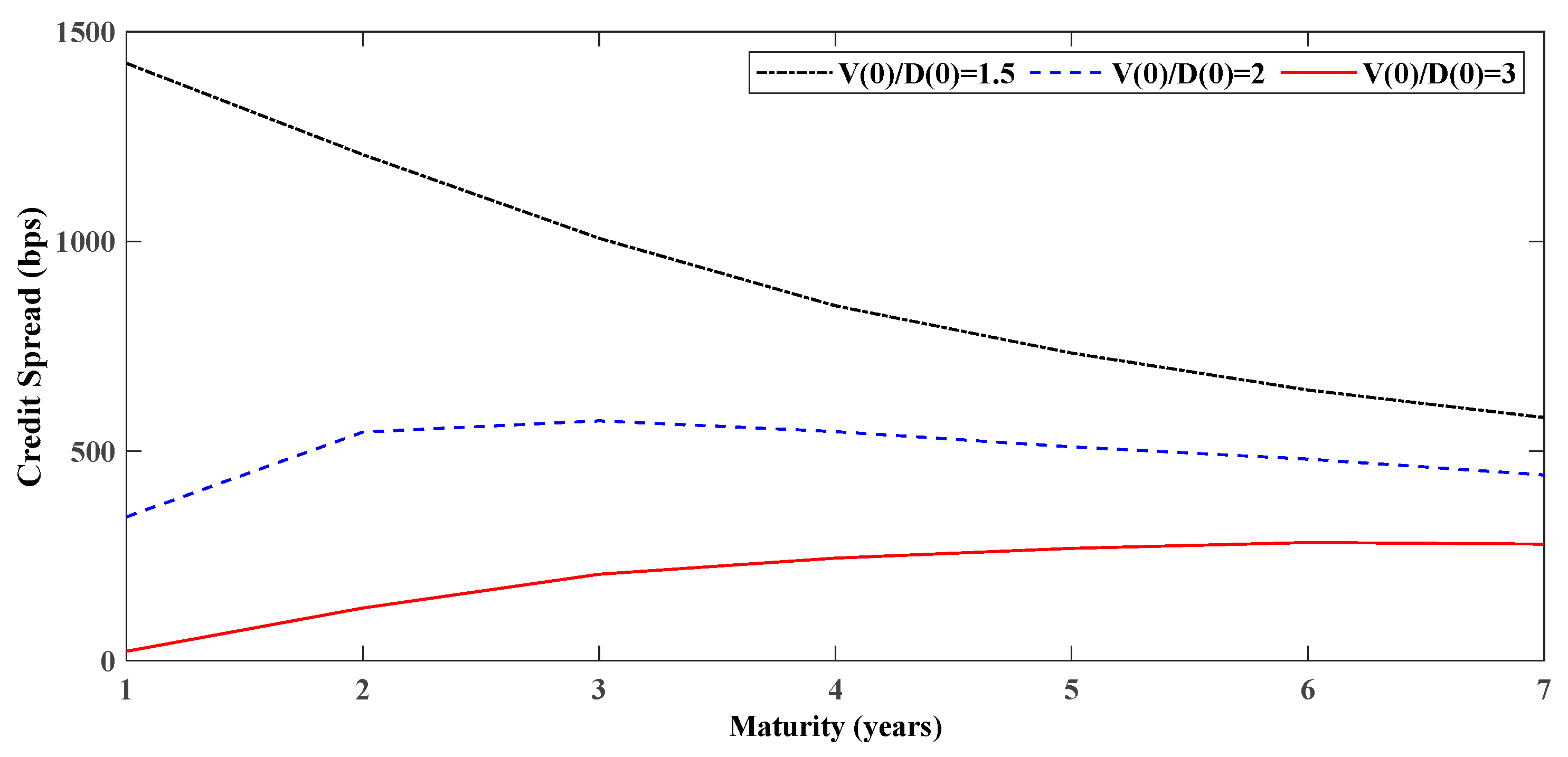
Figure 1. The effect of the ratio of current V ( 0 ) / D ( 0 ) on credit spread. The dash-dotted, dashed, and solid lines correspond to V ( 0 ) / D ( 0 ) = 1.5 , V ( 0 ) / D ( 0 ) = 2 , and V ( 0 ) / D ( 0 ) = 3 , respectively.
Mathematics 13 03628 g001
Figure 2. The effect of the ratio of current V ( 0 ) / D ( 0 ) on default probability. The dash-dotted, dashed, and solid lines correspond to V ( 0 ) / D ( 0 ) = 1.5 , V ( 0 ) / D ( 0 ) = 2 , and V ( 0 ) / D ( 0 ) = 3 , respectively.
Mathematics 13 03628 g002
Figure 3. The effect of the long-term volatility σ 1 , σ 2 on credit spread. The dash-dotted, dashed, and solid lines correspond to σ 1 = 0 . 15 , σ 2 = 0.3 , σ 1 = 0 . 2 , σ 2 = 0.4 , and σ 1 = 0 . 25 , σ 2 = 0.5 , respectively.
Mathematics 13 03628 g003
Figure 4. The effect of the long-term volatility σ 1 , σ 2 on default probability. The dash-dotted, dashed, and solid lines correspond to σ 1 = 0 . 15 , σ 2 = 0.3 , σ 1 = 0 . 2 , σ 2 = 0.4 , and σ 1 = 0 . 25 , σ 2 = 0.5 , respectively.
Mathematics 13 03628 g004
Figure 5. The effect of the jump frequency λ 1 , λ 2 on credit spread. The dash-dotted, dashed, and solid lines correspond to λ 1 = 0 . 05 , λ 2 = 0.1 , λ 1 = 0 . 1 , λ 2 = 0.2 , and λ 1 = 0 . 15 , λ 2 = 0.3 , respectively.
Mathematics 13 03628 g005
Figure 6. The effect of the jump frequency λ 1 , λ 2 on default probability. The dash-dotted, dashed, and solid lines correspond to λ 1 = 0 . 05 , λ 2 = 0.1 , λ 1 = 0 . 1 , λ 2 = 0.2 , and λ 1 = 0 . 15 , λ 2 = 0.3 , respectively.
Mathematics 13 03628 g006
Figure 7. The effect of initial stochastic volatility U ( 0 ) on credit spread. The dash-dotted, dashed, and solid lines correspond to U ( 0 ) = 0.1 , U ( 0 ) = 0.2 , and U ( 0 ) = 0.3 , respectively.
Mathematics 13 03628 g007
Figure 8. The effect of initial stochastic volatility U ( 0 ) on default probability. The dash-dotted, dashed, and solid lines correspond to U ( 0 ) = 0.1 , U ( 0 ) = 0.2 , and U ( 0 ) = 0.3 , respectively.
Mathematics 13 03628 g008
Figure 9. The effect of the ratio of current V ( 0 ) / D ( 0 ) on credit spread and default probability under simplified (upper panel) and generalized (lower panel) conditions. The dash-dotted, dashed, and solid lines correspond to V ( 0 ) / D ( 0 ) = 1.5 , V ( 0 ) / D ( 0 ) = 2 , and V ( 0 ) / D ( 0 ) = 3 , respectively.
Mathematics 13 03628 g009
Table 1. Parameter values.
Parameter NameValue in Boom StateValue in Recession State
Asset value volatility ( σ l )0.150.3
Annual jump intensity ( λ )0.050.1
Double exponential upward jump probability ( p )0.3
Double exponential parameter ( η 1 )1/0.5
Double exponential parameter ( η 2 )1/0.2
Initial value of U 0.1
Drift term of U ( δ )0.03
Volatility term of U ( ν )0.02
Debt volatility ( σ D )0.10.2
Correlation coefficient between asset value and U ( ρ )0.010.02
Correlation coefficient between asset value and debt ( ρ V D )0.050.1
Risk-free rate ( r )0.050.025
Notes: Calculations of values on defaultable bond are according to the parameters shown in Table 1 unless otherwise noted. Additionally, ξ ( t ) = [ 0 , 1 ] is the “boom” state and ξ ( t ) = [ 0 , 1 ] is the “recession” state.
Disclaimer/Publisher’s Note: The statements, opinions and data contained in all publications are solely those of the individual author(s) and contributor(s) and not of MDPI and/or the editor(s). MDPI and/or the editor(s) disclaim responsibility for any injury to people or property resulting from any ideas, methods, instructions or products referred to in the content.