A Novel EMD-1DCNN Framework for Recognizing Concurrent Control Chart Patterns in Autocorrelated Processes

Abstract

Control chart pattern recognition was initially focused on single patterns with the assumption of normal, independent, and identical distribution. In practice, though, these assumptions are rarely valid in manufacturing processes, due to numerous influencing factors and short intervals in data collecting. It is necessary to consider that the inherent disturbance is autocorrelated and that two single patterns appear at the same time. This study presents a novel framework integrating Empirical Mode Decomposition (EMD) and one-dimensional Convolutional Neural Networks (1DCNN) with feature component selection for recognizing concurrent control chart patterns in autocorrelated manufacturing processes. We assume the inherent disturbance follows a first-order autoregressive (AR (1)) process and simulate eleven concurrent patterns. Then, the EMD method decomposes the concurrent pattern into a series of feature components, wherein the correlation coefficient is employed as the index by which to select the two feature components. Finally, the selected feature components and raw data are combined to create a feature vector that acts as the input for the 1DCNN model. The simulation results demonstrate that the proposed model achieves a recognition accuracy of 92.39%, outperforming both the singular spectrum analysis–support vector machine (SSA-SVM) and the singular spectrum analysis–random forest (SSA-RF) methods in terms of accuracy and robustness.

1. Introduction

The control chart is a crucial tool to monitor and analyze the quality of a process. The relevant parameters of the process can be monitored in order to analyze whether the process is in control or not, thereby aiding the engineers in improving it. The first control chart was proposed by Shewhart in 1931 [1], followed by the development and application of various other control chart types [2,3]. For example, the $\overline{X}$ and $R$ control charts with upper and lower control limits are commonly used to monitor mean and variance, respectively. If the points of the control chart exceed the upper or lower control limits, a process is considered out-of-control and has the potential for an abnormality to occur. Similarly, a process is also considered out of control, when the points of the control chart meet one of the eight relevant criteria [4]. In these cases, however, no further information helps engineers in searching for the abnormality’s assignable causes. The appearance of control chart patterns (CCPs) provide a means to overcome the limitations of the traditional control chart. First proposed by the Western Electric Company, CCPs include cyclic, trend, shift, and system patterns [5], with different types of abnormal CCPs corresponding to different assignable causes. For example, shift patterns may indicate changes in materials, machinery, or operators, trend patterns may be related to tool wear, and cyclic patterns may stem from power voltage fluctuations [6,7]. The application of control chart pattern recognition (CCPR) is an indispensable way for quickly identifying assignable causes and formulating solutions. It is the basic formula for ensuring high-quality products.

With the rapid development of computer and microprocessor technologies, several machine learning algorithms have been introduced to CCPR, such as the artificial neural network (ANN), support vector machine (SVM), random forest (RF), decision tree (DT), fuzzy systems, etc. Hachicha and Ghorbel [6] reviewed nearly 120 articles written on CCPR from 1991 to 2010 and came to a number of conclusions, including that the assumption of the data model is a critical issue. As most studies have assumed that the observed value is normally, independently, and identically distributed (NIID), future research can thus continue in two directions, considering autocorrelated process and multivariate process. Another major conclusion is that a single CCP is studied by over 92% of the articles reviewed; evidence of the continued phenomenon of CCPR research concentrated on single CCPs [7,8,9,10,11,12,13]. Although the above-mentioned methods have developed to identify single CCPs based on the assumption of the NIID process, this assumption is untenable among modern intelligent manufacturing processes, such as in the chemical, pharmaceutical, and metallurgical industries [4]. At the same time, the high-frequency data acquisition method will result in high autocorrelation between the observed values [14]. The research on single CCPs of autocorrelation processes is limited. Cheng and Cheng employed a neural network as a classifier to identify five abnormal CCPs in the autocorrelation process [15]. Lin, Guh, and Shiue proposed an online CCPR model based on SVM for identifying seven abnormal CCPs for an autocorrelation process [16]. Yang and Zhou suggested an integrated neural network method based on LVQ and BPNN for an autocorrelation process [17]. These studies assumed the process mean follows a first-order autoregressive (AR (1)) model. De La Torre Gutierrez and Pham first considered that inherent distrustance followed the first-order autoregressive (AR (1)) model and applied SVM to recognize CCPs [18]. Li et al. [19] proposed a multi-scale weighted ordinal pattern and ensemble classifier model for small shift scenarios, significantly improving recognition accuracy for autocorrelated data, though it primarily addresses single abnormal patterns rather than concurrent patterns.

Concurrent patterns (i.e., two or more abnormal CCPs occurring simultaneously) commonly exist in a real-world manufacturing process which may be associated with different assignable causes [19,20]. For example, a cyclic pattern (caused by other assignable causes that appear and disappear regularly, such as unstable material) and a trend pattern (caused by the tool wear) occur simultaneously in the industrial turning process [21]. When more than one abnormal pattern occurs, it is difficult to recognize due to the interaction, and applying single pattern recognition schemes will result in poor classification performance. To effectively recognize a concurrent pattern, it is first necessary to recognize each single pattern. In most studies, wavelet transform (WT), independent component analysis (ICA), and singular spectrum analysis (SSA) are used to decompose a concurrent pattern into a single pattern.

While ICA and SSA have been used for concurrent pattern decomposition, they face critical limitations in autocorrelated processes. ICA’s non-uniqueness due to random initializations [22] and SSA’s sensitivity to parameter selection hinder their effectiveness in non-stationary environments [23]. Moreover, these linear methods struggle to separate mixed patterns with nonlinear dependencies such as trend-modulated cyclic vibrations. In contrast, EMD’s adaptive multi-scale decomposition is better suited to capture such complex interactions [24]. Additionally, research on concurrent pattern recognition has grown, but existing methods face significant challenges in handling complex autocorrelated concurrent patterns. For example, reliance on linear decomposition methods like SSA/ICA can struggle to capture nonlinear interactions [25].

At present, when researching concurrent patterns, most studies assume that the observed values follow NIID processes. Guh and Tannock suggested a method to identify concurrent patterns using a back propagation neural network (BPNN), but it had the disadvantage of a long training time [26]. Chen and Lam used WT to separate concurrent patterns, then used ANN as a classifier to recognize patterns [27]. ICA has also emerged as a popular decomposition method for the recognition of concurrent patterns. Wang, Dong, and Kuo [28] proposed a hybrid method based on ICA and decision tree to identify concurrent patterns. Their results show that although this method can recognize six concurrent patterns, the concurrent patterns of upward trend (UT) and upward shift (US) could not be identified properly. Lu, Shao, and Li [22] applied ICA and SVM to identify concurrent patterns in which ICA was utilized for decomposing concurrent patterns and SVM was applied as a classifier, with results showing that the recognition approach performed well. Nevertheless, ICA could not give a unique solution because different solutions are obtained by different initial conditions. SSA is also a common method for decomposing concurrent patterns. Gu et al. [29] combined SSA and learning vector quantization (LVQ) to recognize concurrent CCPs. Xie et al. [23] applied SSA to separate concurrent patterns into two single patterns, and the SVM was employed as a classifier. The results showed that the decomposition performance of the SSA method was better than that of the ICA, but selecting SSA parameters presented as a challenge. Chiu and Tsai [30] studied an online hybrid method based on SSA and RF for recognizing concurrent patterns, where SSA decomposed concurrent patterns into two single patterns. Extracted statistical and shape features were input into SVM for discriminating types of concurrent patterns. Zhang, Yuan et al. [31] developed a mixture method based on fusion feature reduction and multi-class SVM with a fireworks algorithm, which efficiently identified 4 types of concurrent patterns. Zhang et al. [32] further proposed an intelligent method that included two aspects of feature fusion and extreme learning machine (ELM) with parameter optimization. In their study, Bao et al. [7] developed a multi-scale time series classification model called DMP-MDNet. This model fuses multi-receptive field convolutions to enhance global and local feature representation. However, its generalizability to autocorrelated concurrent patterns needs to be verified. The feature vector used to represent concurrent patterns extracted shape features, statistical features, and raw data. The results indicated that fusion features could improve the accuracy of the model.

A review of the relevant literature shows that most of the studies develop single pattern and concurrent pattern recognition approaches based on the assumption of NIID processes. Some consider the autocorrelation process when studying the recognition methods of single patterns. However, very few studies considered both propositions simultaneously, yet concurrent patterns are common in actual manufacturing processes and the inherent disturbance follows the AR (1) model. Proceeding from this premise, this paper aims to develop a model for recognizing concurrent patterns in autocorrelated processes. We utilize the empirical mode decomposition (EMD) method to decompose concurrent patterns into a series of feature components, with a one-dimensional convolutional neural network (1DCNN) as a classifier. At the same time, a correlation coefficient is employed as the index to select two feature components. To ensure the integrity of concurrent pattern features, two feature components and raw data are linearly combined as feature vectors which serve as the input of the classifier.

This study makes three key contributions to the field of CCPR in autocorrelated processes. (1) Novel framework development: We introduce an EMD-1DCNN architecture, the first to integrate adaptive signal decomposition (EMD) and deep learning for recognizing 11 types of concurrent CCPs under AR (1) disturbances. This addresses the gap identified in Garcia et al.’s review [20], which highlighted the lack of data-driven methods for concurrent patterns in autocorrelated systems. (2) Feature fusion strategy: By selecting and combining IMF components via correlation coefficients, we overcome the limitations of linear decomposition methods (e.g., SSA/ICA) in capturing nonlinear interactions between patterns [22,23]. (3) Empirical validation: Through Monte Carlo simulations, we demonstrate that the proposed model achieves 92.39% accuracy, outperforming traditional SSA-based methods by 10–15% in autocorrelated scenarios.

The rest of this paper is established as follows. Section 2 discusses the structure of concurrent patterns of the autocorrelated processes, while Section 3 introduces EMD and CNN methods and Section 4 describes the proposed model. The simulation results of the proposed model, as well as a comparison, are presented in Section 5, with conclusions provided in Section 6.

2. Concurrent CCP in Autocorrelated Processes and Abnormal Disturbance Models

Validating CCPR models requires large sample sizes, but collecting real manufacturing data is challenging due to storage limitations, quality costs, and the low frequency of abnormal patterns (which often trigger immediate shutdowns or maintenance). Simulation methodology thus remains the mainstream method for generating CCPs.

Firstly, an autocorrelated process model is established. The inherent disturbance is represented by an AR (1) model (De La Torre Gutierrez and Pham 2018 [18]), and the mathematical expressions are given:

$$Y_t=\mu +N_t+D_t$$

(1)

$$N_t=\phi N_{t-1}+e_t, e_t\sim N(0,1)$$

(2)

where $Y_t$ is the observed value at time $t$ in manufacturing processes, $\mu$ is the mean of observations when the manufacturing process is in control, $N_t$ is inherent disturbance at time $t$, and obeys AR (1) model, $D_t$ is abnormal disturbance at time $t$, $\phi$ is the autocorrelation coefficient, and set $0<\phi \le 0.3$. $e_t$ is a random variable, and obeys normal distribution.

The formulas for the types of abnormal disturbance patterns (trend, shift, cyclic, and system patterns) have their formulas are expressed as follows.

(1)

Upward and Downward Trend patterns (UT/DT)

$$D_t=\pm {\gamma }_1\times t$$

(3)

where ${\gamma }_1$ represents the slope of a trend, the UT pattern uses the sign “$+$”, and the DT pattern uses the sign “$-$”.

(2)

Upward and Downward Shift patterns (US/DS)

$$D_t=\pm {\gamma }_2\times d$$

(4)

where ${\gamma }_2$ represents the shift magnitude, $d$ represents shift point, $d$ is equal to 0 before the shift and to 1 after the shift, US pattern uses the sign “$+$”, and DS pattern uses the sign “$-$”.

(3)

Cyclic pattern (CYC)

$$D_t=\pm {\gamma }_3\times \sin \left({\displaystyle \frac{2\pi t}{{\gamma }_4}}\right)$$

(5)

where ${\gamma }_3$ and ${\gamma }_4$ represent the amplitude and period of a cycle, respectively.

(4)

System pattern (SYS)

$$D_t={\gamma }_5\times {\left(-1\right)}^t$$

(6)

where ${\gamma }_5$ represents a systematic departure.

In this study, the concurrent patterns are generated by a linear combination of single abnormal patterns. The formula is expressed as follows:

$$Y_t=\mu +N_t+D_{1,t}+D_{2,t}$$

(7)

where $D_{1,t}$ represents abnormal disturbance 1, and $D_{2,t}$ represents abnormal disturbance 2. The selection of two disturbance components is justified by two key reasons: (1) Industrial practice: Most concurrent abnormal scenarios in manufacturing (e.g., turning processes, chemical batches) involve two overlapping patterns (e.g., cyclic + trend, shift + cyclic), while three or more concurrent patterns are extremely rare (Yang and Zhou, 2015 [21]; Garcia et al., 2022 [20]). (2) Literature consistency: Prior studies on concurrent CCPR (Xie et al., 2013 [23]; Wang et al., 2009 [28]) primarily focus on two-component combinations, as adding a third component would significantly increase computational complexity without substantial improvement in practical recognition value. Omitting disturbance components (i.e., using raw data alone) would lose critical pattern details, leading to low accuracy (see Section 5.4 for verification).

In the literature, Wang, Dong, and Kuo, studied six types of concurrent patterns [28], while Gu et al., 2013 [29] and Xie et al., 2013 [23] researched nine In our work, we consider 11 types of concurrent patterns, including CYC + UT, CYC + DT, CYC + SYS, US + CYC, DS + CYC, US + UT, US + SYS, DS + SYS, DS + DT, SYS + UT, and SYS + DT. There are 11 types of concurrent patterns shown in Figure 1. The emergence of a concurrent pattern means that the abnormality may have several causes within the manufacturing process. In order to more rapidly detect the abnormal causes, it is necessary to identify the single patterns from the concurrent patterns. For more information on abnormal causes, please refer to Reference [24].

To ensure the facticity of the simulated samples, the parameters of CCPs are set in a large range and are consistent with the literature [33]. Without loss of generality, $\mu$ is set to 0. The parameters of abnormal patterns follow the uniform distribution.

Table 1. Parameters of abnormal patterns.

Pattern Type	Formula	Parameters
Upward Trend (UT)	$Y_t=u+N_t+{\gamma }_1\times t$	${\gamma }_1~\mathrm{U} (0.1,0.3)$
Downward Trend (DT)	$Y_t=u+N_t-{\gamma }_1\times t$	${\gamma }_1~\mathrm{U}(0.1,0.3)$
Upward Shift (US)	$Y_t=u+N_t+{\gamma }_2\times d$	${\gamma }_2~\mathrm{U} (0.1,3.0)$
		$15\le d\le 45$
Upward Shift (DS)	$Y_t=u+N_t-{\gamma }_2\times d$	${\gamma }_2~\mathrm{U} (0.1,3.0)$
		$15\le d\le 45$
Cycle (CYC)	$Y_t=\mu +N_t+{\gamma }_3\times \sin \left({\displaystyle \frac{2\pi t}{{\gamma }_4}}\right)$	${\gamma }_3~\mathrm{U} (0.1,3.0)$
		${\gamma }_4~\mathrm{U} (3,16)$
Systematic (SYS)	$Y_t=u+N_t+{\gamma }_5\times {\left(-1\right)}^t$	${\gamma }_5~\mathrm{U}(0.1,3.0)$

shows the parameters of abnormal patterns. The rationale for parameter ranges is as follows: (1) Shift magnitude (${\gamma }_2$), cyclic amplitude (${\gamma }_3$), and systematic departure (${\gamma }_5$) share the same range U (0.1, 3.0) because De La Torre Gutierrez and Pham 2016 [33] demonstrated that this interval covers 90% of abnormal deviation magnitudes in autocorrelated manufacturing processes; (2) trend slope (${\gamma }_1~$U(0.1, 0.3)) is set to a smaller range to avoid overshadowing other patterns (Yang and Zhou, 2015 [21]); (3) cyclic period (${\gamma }_4~$U (3, 16)) aligns with common industrial cycle intervals (e.g., power voltage fluctuations, tool wear cycles) (Xie et al., 2013 [23]). The window length N is set to 60. A total of 26,400 samples are generated, with a balanced split: 17,600 for training, 4400 for validation, and 4400 for testing (1600/400/400 samples per concurrent pattern, avoiding class imbalance). All samples are generated via Monte Carlo simulation based on the AR (1) disturbance model, consistent with the parameter settings in De La Torre Gutierrez and Pham [18,33]. No real experimental data is used due to the rarity of concurrent abnormal patterns in actual manufacturing processes, which is a common practice in CCPR research [20,23].

3. Methodology

3.1. EMD and Correlation Coefficient

The Empirical Mode Decomposition (EMD), proposed by Huang et al. (1998) [34], is a data-driven adaptive signal decomposition technique designed for nonlinear and non-stationary time series. Its core principle is to decompose a signal into a set of Intrinsic Mode Functions (IMFs) and a residual (R), where each IMF represents a distinct oscillatory mode of the signal, and the residual reflects the overall trend or DC component. This section supplements the underlying theory of EMD, IMF criteria, and step-by-step decomposition procedures to enhance reproducibility.

The EMD, proposed by Huang et al. [34], is a data-driven signal decomposition method. As a new method of adaptive signal processing, EMD can decompose time series into Intrinsic Mode Function (IMF) components and a Residual (R) component. For a component to be classified as an IMF, it must satisfy two strict criteria (Huang et al., 1998 [34]): (1) Throughout the entire time series, the number of local extrema (maxima + minima) and the number of zero-crossings must be equal or differ by at most 1. (2) At any time t, the mean value of the upper envelope (fitted by cubic spline interpolation of local maxima) and the lower envelope (fitted by cubic spline interpolation of local minima) must be zero. These criteria ensure that IMFs are narrowband signals with physically meaningful oscillatory characteristics.

Compared with other decomposition methods, such as WT, ICA, and SSA, the EMD has obvious advantages. First, it can directly decompose data without the need for prior analysis or research. Second, it automatically divides into layers according to some inherent modes without requiring human intervention. This makes the EMD particularly suitable for control chart patterns with mixed trends, cycles, and shifts—common in autocorrelated manufacturing processes (e.g., chemical batch systems).

The IMF component has two main specifications: the number of local extremes and the number of zero-crossings must be equal or differ by 1 at most in the whole time range; additionally, at any time, the means of the envelope defined by local maximum and minimum shall be equal to 0. The original data is decomposed into a series of IMF and R components, which can be expressed as follows:

$$Y(t)={\displaystyle \sum _{i=1}^{n}IM{F}_i(t)+R(t)}$$

(8)

where $Y(t)$ is raw data, $n$ is the number of IMF components, $IM{F}_i(t)$ is the $i$th component, and $R(t)$ is the residual component.

The EMD process for a signal $Y(t)$ follows these detailed steps (Huang et al., 1998 [34]; Zhang et al., 2021 [35]):

(1)

Find all maximum points of a signal $Y(t)$ and use cubic spline interpolation to fit the upper envelope of the original data.

(2)

Find all minimum points of a signal $Y(t)$ and use cubic spline interpolation to fit the lower envelope of the original data.

(3)

$Y(t)$ minus the mean of the upper and lower envelope, a component $f_1(t)$, is obtained using the following equation.

$$f_1(t)=Y(t)-m_1(t)$$

(9)

(4)

Determine whether $f_1(t)$ satisfies the requirement of IMF. If yes, $f_1(t)$ is used as the $IM{F}_1$ component. Otherwise, repeat steps (1)–(3) until the $k$th meets the requirement. The formulation is given by

$$IM{F}_1=f_{1k}(t)=f_{1(k-1)}(t)-m_{1k}(t)$$

(10)

(5)

$Y(t)$ minus $IM{F}_1$ for obtaining $R(t)$. Then let $R(t)$ repeat steps (1)–(3) and determine whether the requirement is satisfied. If necessary, repeat the above steps. Otherwise, stop decomposition.

Regarding the observation that all patterns yield only two IMFs and one residual, this is a natural outcome of EMD’s adaptive mechanism for concurrent CCPs. Since each concurrent pattern is composed of two single abnormal patterns (e.g., CYC + UT, US + CYC), the signal contains two dominant frequency scales (e.g., high-frequency cyclic oscillations and low-frequency trend). EMD automatically identifies these two scales and extracts them as two IMFs, while the residual captures the remaining trend or DC component. No decomposition level is predetermined—this result aligns with EMD’s ability to match decomposition depth to signal complexity (Huang et al., 1998 [34]; Zhang et al., 2021 [35]). The one-dimensional raw data are divided into a series of IMF and R components effectively expressing the features of the raw data at different scales. To select the components with obvious features, the correlation coefficient is expressed by the following formula:

$$r_i(X_i,Y(t))={\displaystyle \frac{\mathrm{cov}(X_i,Y(t))}{\sqrt{\mathrm{var}(X_i)\times \mathrm{var}(Y(t))}}}$$

(11)

where $X_i$ represents the $IM{F}_i$ or $R(t)$ component.

The correlation coefficient was chosen as the selection metric due to its simplicity and effectiveness in capturing linear dependence between components and raw data. Preliminary experiments with mutual information and variance contribution showed comparable performance but higher computational cost. Thus, the correlation coefficient balances accuracy and efficiency for feature component selection.

3.2. Convolutional Neural Network

CNN is a deep feedforward neural network in which mainly the convolution layer and pooling layer complete feature extraction, selection, and optimization [35]. Because CNN has better self-learning ability, it can solve more complex problems without the need for data pre-processing, as raw data is used directly to train and test the model [36]. Another advantage of CNN is its automatic feature extraction, which improves the integrity and stability of extracted features. The major structure of CNN is described as follows.

A convolutional layer uses the convolution kernel to perform a series of convolution operations. The expression of convolution operation is given by

$${\mathit{x}}_j^l=f({\displaystyle \sum _{i=1}^{G_{l-1}}{\mathit{x}}_i^{l-1}\ast {\mathit{k}}_{ij}^l}+{\mathit{a}}_j^l)$$

(12)

where $x_j^l$ is the $j$th output feature map, $l$ represents the serial number of current network layer, $f$ means an activation function, $G$ is the number of features, $\ast$ means convolution operation, $k^l$ is convolution kernel, and $a_j^l$ means the additive bias.

The ReLU activation function is employed in this paper, which can be expressed by

$$f(x)=\max (0,x)$$

(13)

The dimension of the raw data changes after convolution, and its formula is expressed as follows:

$$H_l\times W_l=[(H_l-h)/s+1]\times [(W_l-w)/s+1]$$

(14)

where $H$ and $W$ represent the height and width of the output feature map in the convolution layer, $h$ and $w$ are the height and width of the convolution kernel, and $s$ is the moving stride of the convolution kernel set as 1 in this paper.

The pooling layer is simpler than the convolution layer and has several functions, such as reducing the dimension of features, improving the calculation speed of the model, and enhancing its robustness. In our work, we have adopted the max-pooling strategy to preserve the prominent features, which is defined by the following equation:

$${\mathit{x}}_j^l=down\left({\mathit{x}}_j^{l-1}\right),j=1,2,\cdot \cdot \cdot ,G_l$$

(15)

where $G^l$ means the number of input feature maps and $down$ represents the pooling function.

The dimension of the output feature map is further reduced after the pooling operation. The calculation formula is shown as follows:

$$H_l\times W_l=(H_{l-1}/u)\times (W_{l-1}/u)$$

(16)

where $u$ means the step size of the pooling operation and is equal to 2 in this paper, chosen based on trade-off between feature retention and computational efficiency, which is consistent with common settings in 1DCNN for time-series classification [35].

After a series of convolution and pooling operations, the feature maps are expanded and spliced together in the fully connected layer. The equation is given by

$${\mathit{x}}_i=f({\mathit{\omega }}_0{\mathit{f}}_v+{\mathit{b}}_0)$$

(17)

where ${\mathit{f}}_v$ represents the input vector, ${\mathit{\omega }}_0$ represents weight matrix, and ${\mathit{b}}_0$ represents a vector of the bias.

To obtain the prediction outcome of the model, the Softmax function is applied to realize multi-classification. The $f(x_i)$ is defined as:

$$f(x_i)={\displaystyle \frac{e^{x_i}}{{\displaystyle \sum _{i=1}^M{e}^{x_j}}}}$$

(18)

where $M$ is the number of training samples.

This paper applies the Cross Entropy Loss Function to minimize the loss rate of the model. It is defined by

$$J(\theta )=-{\displaystyle \sum _{k=1}^M{h}_k\log f_k(\theta )}$$

(19)

where $\theta$ is training parameters of the model, $h_k$ is output category of the $k$th objective, $f_k(\theta )$ is prediction probability of the $k$th samples, and $J(\theta )$ is the loss value.

In this study, we employ the Batch Normalize (BN) layer after the convolution layer because of several advantages First, this makes the features obey a normal distribution, while also eliminating the difference in data distribution, overcoming the gradient disappearance problem and improving the training speed. If there is an obtained $w$-dimensional vector after the convolution layer, $X=(x_1,x_2,x_3,\cdot \cdot \cdot ,x_w)$ with $w$-dimensional will be the input of the BN layer. To reduce the transfer of internal covariance, every feature is normalized as

$${\widehat{x}}_i={\displaystyle \frac{x_i-\mathrm{E}(x_i)}{\sqrt{\mathrm{var}(x_i)}}}$$

(20)

where $\mathrm{E}(x_i)$ is the mean of the $x_i$, and $\mathrm{var}(x_i)$ is the variance of the $x_i$.

Keep in mind, however, that transformation of Formula (20) will lead to a decline in network expression ability. Every neuron needs to add two parameters (${\alpha }_i$ and ${\beta }_i$) for adjusting the normalized feature. The expression of the process is given by

$$h_i={\alpha }_i\widehat{x}+{\beta }_i$$

(21)

4. Proposed EMD-1DCNN Model Based on Feature Component Selection

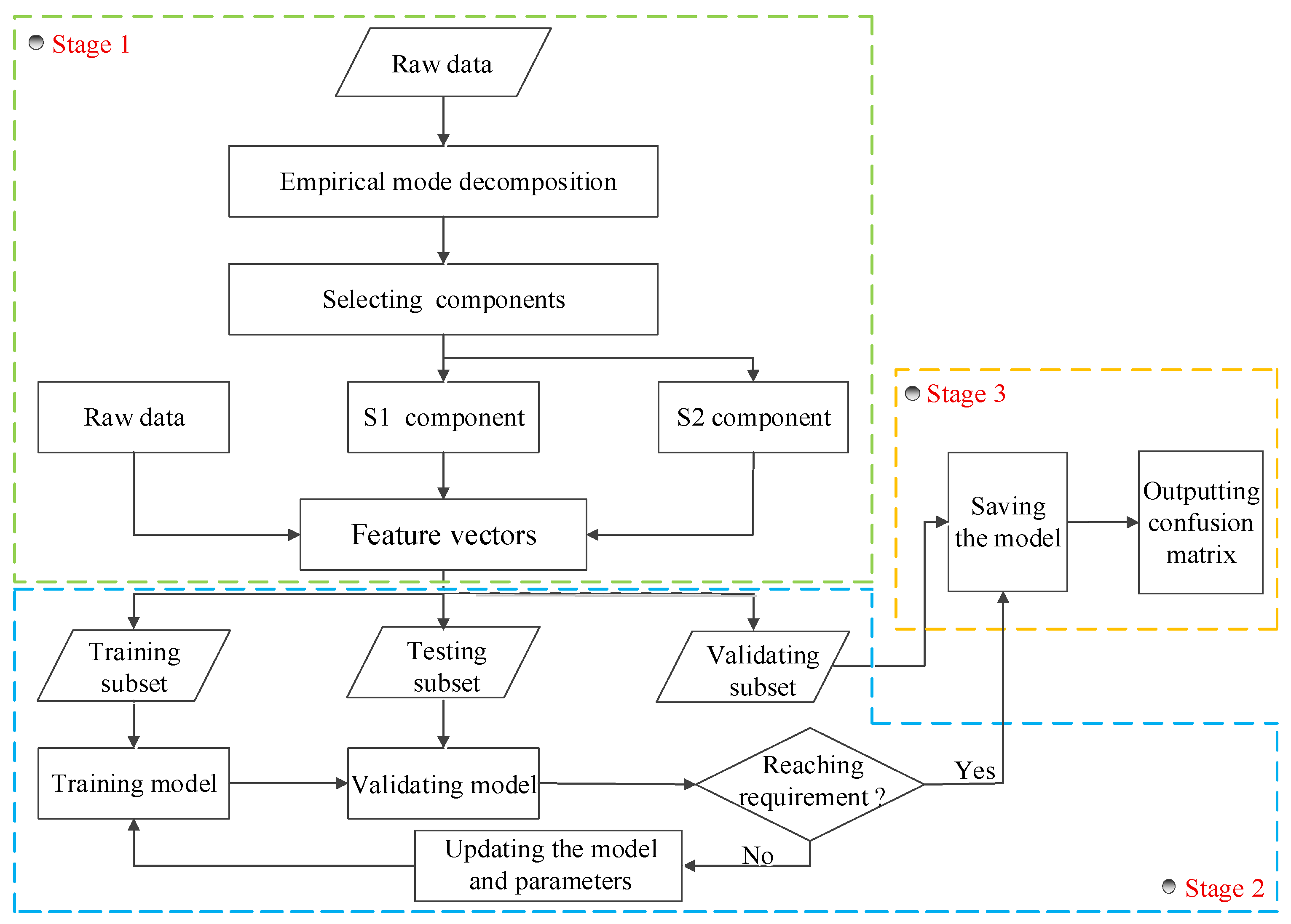
In this paper, we propose an EMD-1DCNN model based on feature component selection to recognize concurrent patterns in autocorrelated processes. The flow diagram of the proposed CCPR model is shown in Figure 2. The model comprises three main stages. Stage 1 includes generation, decomposition, selection, and reconstruction of raw data. In this stage, the Monte Carlo simulation algorithm is used to generate 11 types of concurrent patterns, and EMD is utilized to decompose the concurrent CCP into a series of IMF and R components. Since every component contains different features of raw data, this paper suggests calculating the correlation coefficients between each component and the raw data for selecting two components (S1 and S2) with obvious features. The relationship between S1/S2 and EMD components (IMF1, R) is clarified in that S1 and S2 are not arbitrary EMD components, but the two components with the highest correlation coefficients to the raw data (typically IMF1 and Residual, see

Table 2. Correlation coefficients between components and raw data (CYC + UT pattern).

Component	Correlation Coefficient ($\mathit{\rho }$) with Raw Data	Selection Result
IMF1	0.5927	Selected (S2)
IMF2	−0.0144	Discarded
Residual	0.7620	Selected (S1)

). Unlike direct addition of IMF1 + IMF2 + R (which includes low-correlation noise components like IMF2), S1/S2 are “feature-enhanced components” that retain only the critical pattern information. When combined with raw data, the input vector integrates both the original signal and the key decomposed features—this differs from “raw data + random EMD components” by avoiding redundancy and noise interference, thus improving model accuracy (see Section 5.4 for verification). A larger correlation coefficient indicates that the component contains more features of raw data, allowing S1, S2, and the raw data to combine into a new feature vector. In stage 2, a 1DCNN model is constructed. The feature vectors are input into the 1DCNN model for training, validation, and testing. The 1DCNN structure comprises the contents outlined in Section 3.2. The structures and parameters are adjusted according to validation results. By comparing the accuracy of different structures and parameters, a better 1DCNN model is obtained. In stage 3, the 1DCNN model is employed as the classifier to identify 11 types of concurrent CCPs. The performance of the classifier is validated by the test set. The final recognition performance is represented in the form of a confusion matrix.

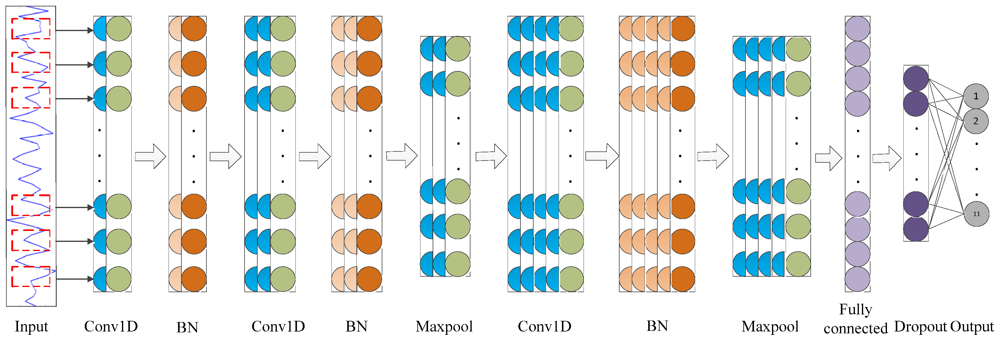
The structure of 1DCNN based on the BN layer is shown in Figure 3, which includes the input layer, three convolution layers, two pooling layers, three BN layers, one full connection layer, one dropout layer, and an output layer. The convolution and pooling layers are used to select, extract, and optimize features for gaining depth features. Because the pooling layer does not change the distribution of features, the BN layer is only applied after the convolution layer, and the dropout layer is introduced to avoid overfitting. After gaining the depth features, the full connection layer completes feature fusion and reduces computation. Finally, the Softmax classifier realizes classification in the output layer.

5. Experiments

In this section, a sequence of simulation experiments is conducted to validate effectiveness of the proposed method. The accuracy of the test samples is used as the evaluation criterion, and the accuracy of each concurrent pattern is intuitively represented by the confusion matrix. Then, the performance of the proposed model is validated through the comparison with the other methods suggested by the previous research.

5.1. EMD and Component Selection

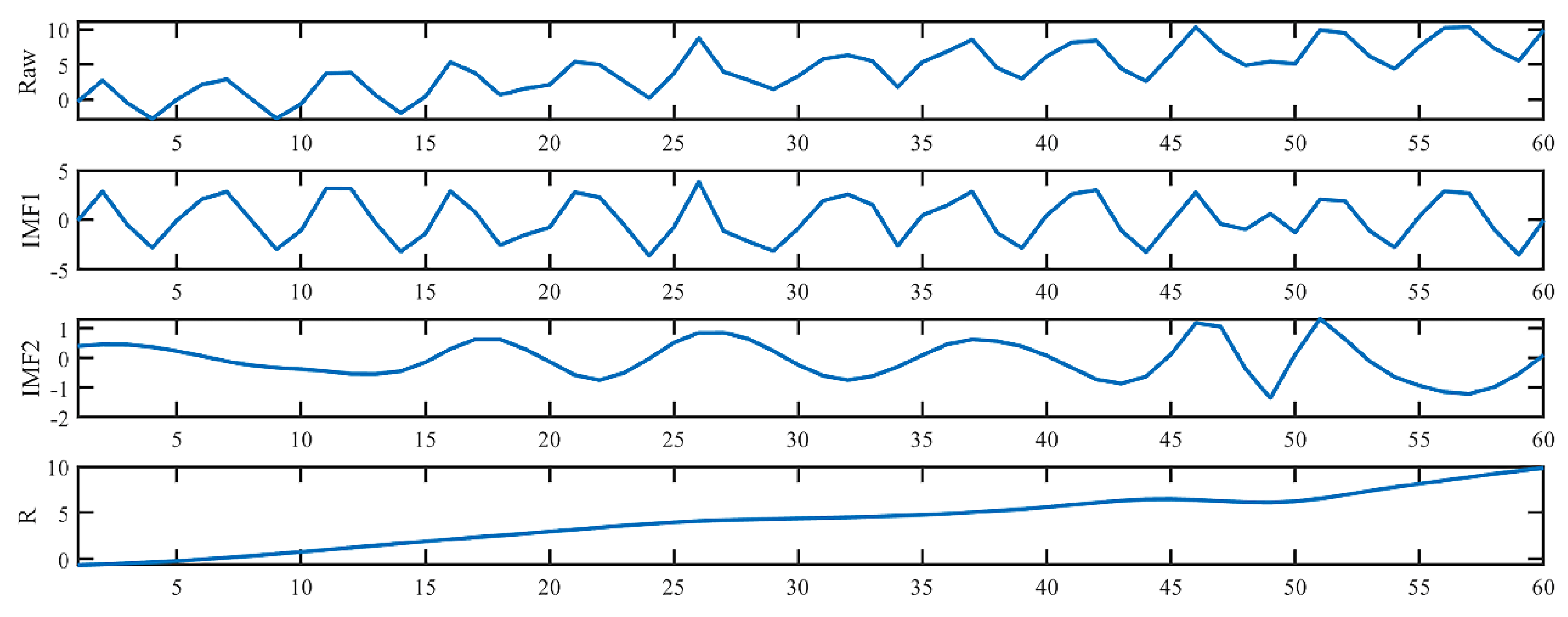
The EMD method decomposes concurrent CCP into a series of IMF and R components which can express features of concurrent patterns in different scale details. Taking the CYC + UT pattern as an example, the raw data and three feature components are shown in Figure 4. The two IMFs contain a great deal of information about the CYC, and the R component represents the slope of the UT pattern.

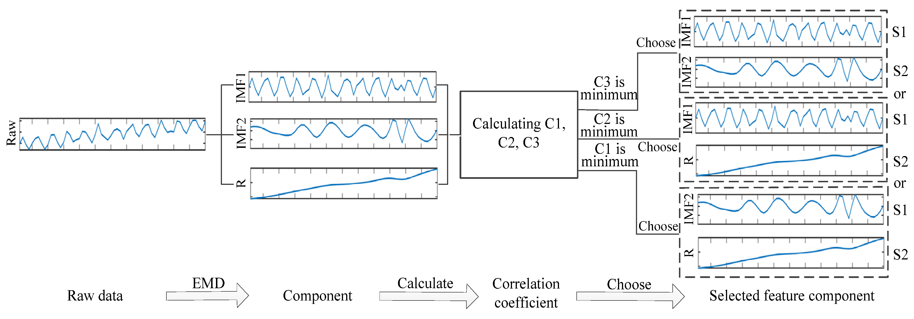
In this paper, the correlation coefficient is adopted as the selection index for S1 and S2 components, which are highly correlated with raw data. The selection detail of S1 and S2 components is shown in Figure 5. At first, raw data is decomposed into IMF and R components. Then, C1, C2, and C3 are calculated according to Formula (11). C1 is the correlation coefficient between IMF1 and Raw data. C2 represents the correlation coefficient between IMF2 and Raw data. C3 means the correlation coefficient between IMF2 and Raw data. The correlation coefficients between each component and raw data (taking CYC + UT pattern as an example) are provided in Table 2 (previously missing), which clarifies the selection basis of S1 and S2. C1, C2, and C3 are equal to 0.5927, −0.0144, and 0.7620, respectively. As a result, both IMF1 and R components are selected as S1 and S2 feature components. Finally, the feature vectors S1, S2, and Raw data are combined linearly, and used as the input of the classifier.

5.2. Structural Parameters of 1DCNN

In this paper, 1DCNN based on BN is employed as a classifier for identifying the concurrent CCPs, with the batch size set to 40 to balance training stability and speed. Moreover, we employed an Adam optimizer to adjust the learning rate. The length of the feature vector was 120 in the input layer, and the training and validating subsets were iterated 100 times to ensure convergence without overfitting. The structure and parameters of 1DCNN were also repeatedly adjusted to obtain an optimal model. The structural parameters of 1DCNN are shown in

Table 3. Structural parameters of the 1DCNN.

Structure	Parameter and Value
Input	$G_1\times H_1\times W_1=1\times 120\times 1$
Conv1D	$G_2\times H_2\times W_2=8\times 118\times 1$
	$h_2\times w_2=3\times 1$
BN	--
Conv1D	$G_3\times H_3\times W_3=16\times 116\times 1$
	$h_3\times w_3=3\times 1$
BN	--
Maxpool	$G_4\times H_4\times W_4=16\times 58\times 1$
Conv1D	$G_5\times H_5\times W_5=32\times 56\times 1$
	$h_5\times w_5=3\times 1$
BN	--
Maxpool	$G_6\times H_6\times W_6=32\times 28\times 1$
Fully connected	M = 896
Dropout	P = 0.5
Output	N = 11

, in which M represents the number of features in a fully connected layer, P is the rejection rate of the dropout layer, and N is the number of the category. We selected ReLU as the activation function and the “Same” function was applied for edge processing in all convolution layers in this paper.

5.3. Results

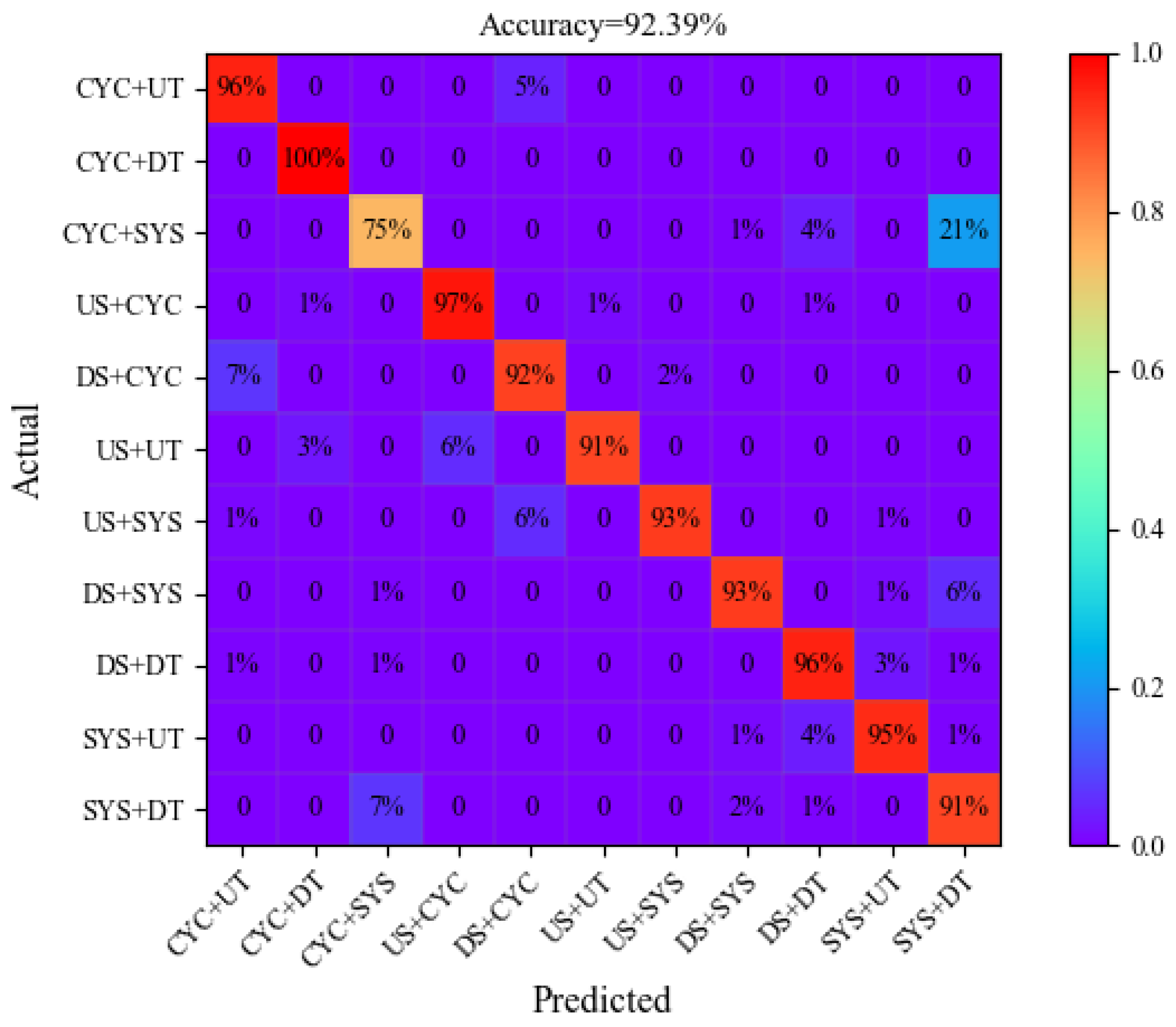
This subsection presents the experimental result of the proposed model. To display the details of the recognition for each pattern, the confusion matrix of the proposed model is given in Figure 6. The accuracy is indicated in the diagonal of the confusion matrix for each pattern, while the other values represent the error recognition rates. For instance, the 97% value in the fourth line represents the accuracy of the US + CYC, and the value of 1%, 1%, and 1% denotes that this type is falsely diagnosed as CYC + DT, US + UT, and DS + DT patterns, respectively. The title of the confusion matrix shows that the average accuracy of the 11 types of concurrent patterns is 92.39%. Notably, all patterns, except CYC + SYS (74.75%), achieve an accuracy of over 90%, demonstrating the model’s strong recognition ability.

Figure 7 shows the variation curves of accuracy and loss for the training and validation sets. The training accuracy increases steadily with the number of epochs, while the validation accuracy stabilizes at approximately 93%, and there is no significant gap between training and validation accuracy—indicating no overfitting and good model generalization.

5.4. Discussion

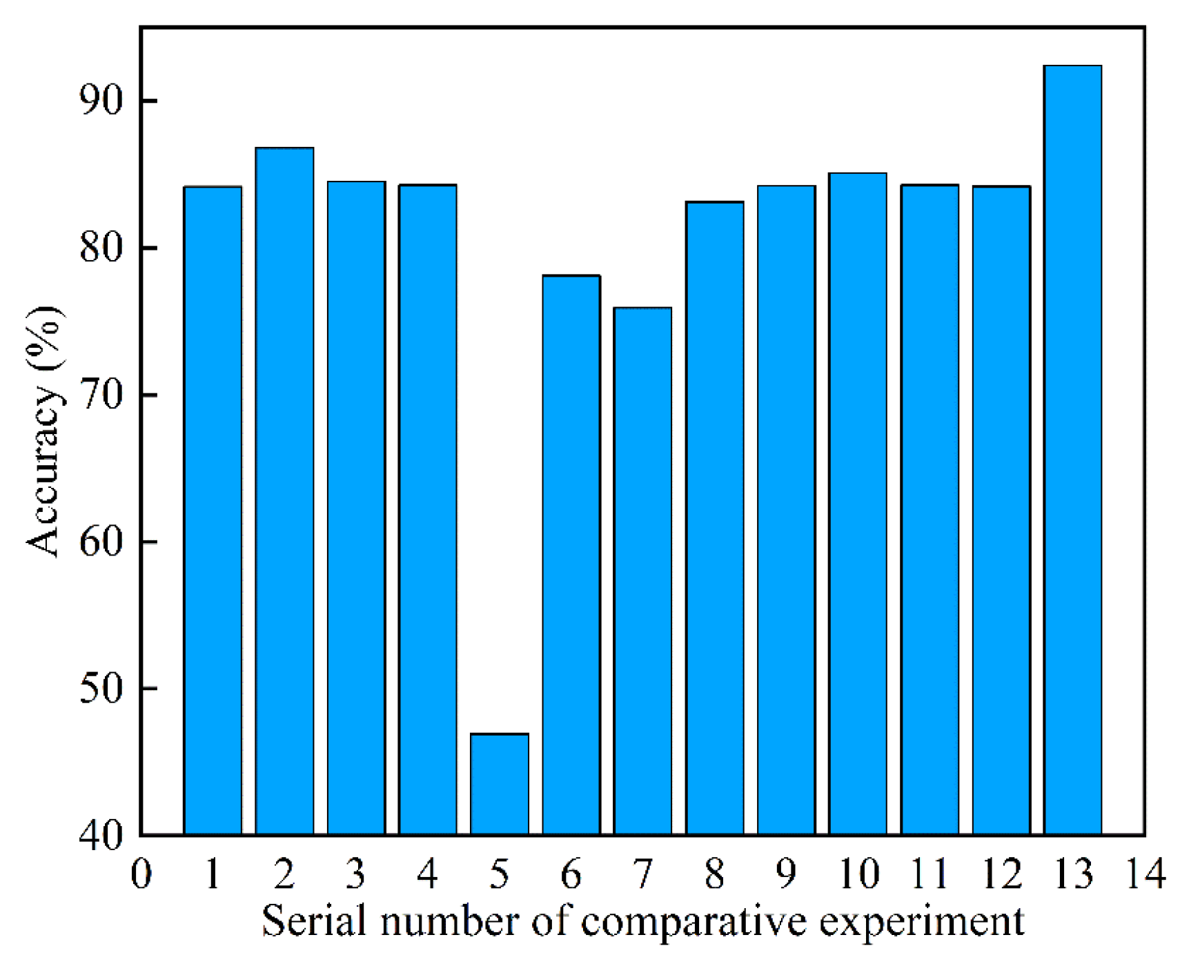
Initially, thirteen comparative experiments are conducted to validate the effectiveness of selecting S1 and S2 components, with the results displayed in

Table 4. The recognition accuracy of the comparative experiments.

Number	Feature Vector	Accuracy	Number	Feature Vector	Accuracy
1	Raw	84.14%	8	IMF1 + IMF2 + R	83.12%
2	Raw + IMF1	86.79%	9	Raw + IMF1 + IMF2	84.22%
3	Raw + IMF2	84.48%	10	Raw + IMF1 + R	85.07%
4	Raw + R	84.27%	11	Raw + IMF2 + R	84.25%
5	IMF1 + IMF2	46.94%	12	Raw + IMF1 + IMF2 + R	84.16%
6	IMF1 + R	78.09%	13	Raw + S1 + S2	92.39%
7	IMF2 + R	75.92%

and Figure 8. The apparent inconsistency in Table 4 (e.g., 84.14% for Raw vs. 83.12% for Raw + IMF1 + IMF2 + R) is explained by the “noise interference effect”. Adding IMF2 (correlation coefficient = −0.0144) introduces irrelevant noise that offsets the useful information from IMF1 and R, leading to lower accuracy than raw data alone. In contrast, Raw + S1 + S2 (92.39%) avoids this issue by selecting only high-correlation components, which enhances critical features without redundant noise. This aligns with feature selection theory (Zhang et al., 2021 [35]), where “quality over quantity” of features determines model performance. It is observed that the recognition performance of the classifier varies depending on the feature vectors used as input. When the raw data is input into the classifier, the accuracy reaches 84.14%. The results of other experiments in which components and raw data are randomly combined as input are lower than the result based on feature component selection. In contrast to the thirteen experiments mentioned above, S1, S2, and raw data can effectively demonstrate the characteristics of the concurrent pattern. Results show that the accuracy increases from 84.14% with raw data to 92.39% with feature component selection, indicating the promising performance of selecting and combining feature components.

Secondly, to verify the performance of the 1DCNN classifier, three experiments are conducted to compare the accuracy of different classifiers, including SVM and RF classifiers. The RBF function is selected as the kernel function in SVM, with the parameters of RF shown in

Table 5. The parameters in RF.

Parameters	n_Estimators	Max_Depth	Min_Samples_Leaf	Min_Samples_Split
Values	100	20	1	20

. Figure 9 gives the confusion matrices of different classifiers to identify feature vectors. The classification performance of 1DCNN clearly exceeds both SVM and RF, with the accuracy of 1DCNN being 92.39%, and SVM and RF being 86.36% and 88.75%, respectively. This advantage arises from 1DCNN’s ability to automatically learn high-level features from time-series data, whereas SVM and RF rely on manual feature engineering.

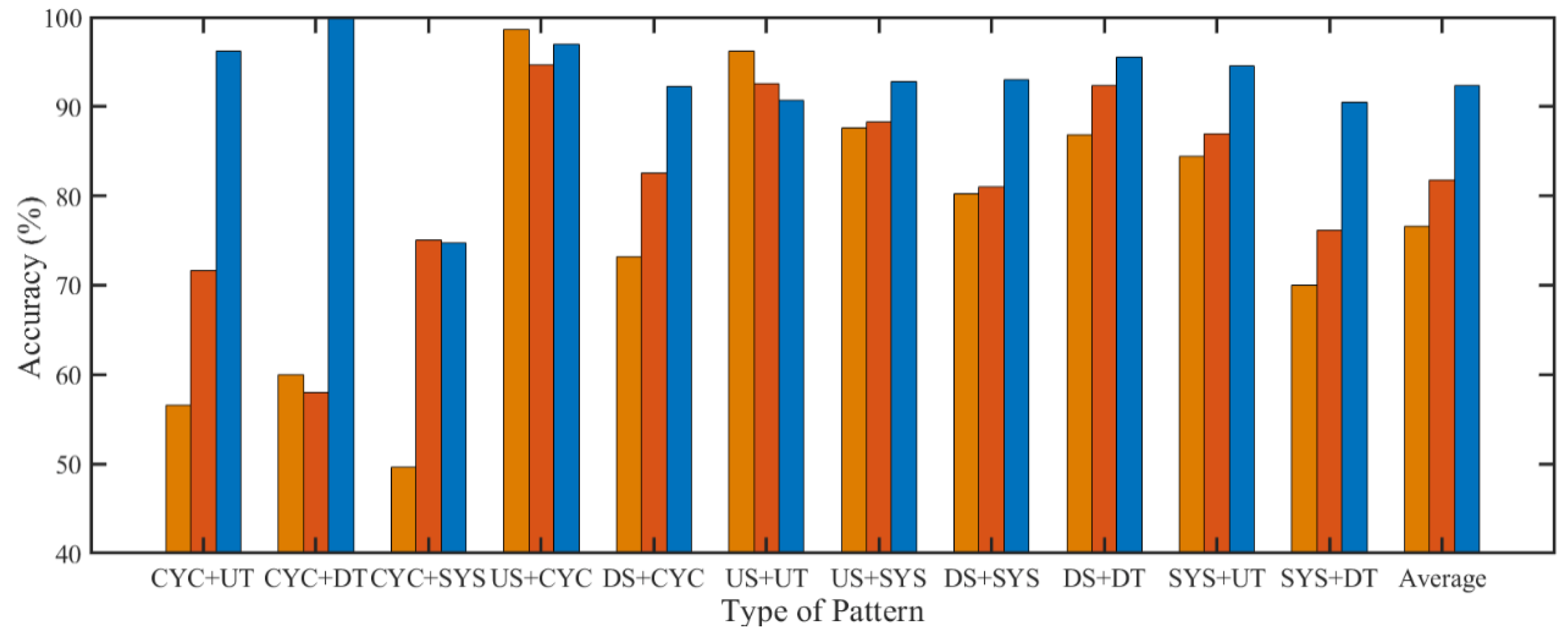
Finally, comparative experiments are implemented between our model and the two other methods to prove the effectiveness of the proposed method. One is the SSA-SVM scheme proposed by Xie et al. (2013) [23], and the other is the SSA-RF scheme proposed by Chiu and Tsai (2021) [30]. Figure 10 demonstrates the results of the proposed model and the two other methods. The results show that the average accuracy of the SSA-SVM method and the SSA-RF method are 76.65% and 81.75%, respectively, significantly lower than the proposed model’s 92.39% accuracy. The accuracy of each pattern of the EMD-1DCNN model is expected to surpass that of the SSA-SVM and SSA-RF methods overall. However, the SSA-SVM method demonstrates better accuracy for US + CYC and US + UT patterns, with a 2.1% and 5.45% higher accuracy compared to the EMD-1DCNN model, respectively. The SSA-RF method, which has better accuracy for CYC + SYS and US + UT patterns, is 0.3% and 1.82% higher than the EMD-1DCNN model. Therefore, it is clear that the proposed model performs well in terms of the average accuracy of eleven concurrent patterns among these three models.

6. Conclusions

CCPR is vital for ensuring process stability in complex manufacturing environments, where concurrent abnormal patterns often signal multi-source issues. This study’s key findings are summarized as follows: (1) A novel EMD-1DCNN framework is proposed for concurrent CCPR in autocorrelated processes, which integrates EMD-based feature selection and 1DCNN classification. (2) The framework recognizes 11 types of concurrent patterns with 92.39% accuracy, outperforming SSA-SVM (76.65%) and SSA-RF (81.75%) by 10–15%. (3) Feature selection via correlation coefficients (selecting S1/S2 from EMD components) is critical for accuracy improvement, as it avoids noise interference from low-correlation components. This study presents an EMD-1DCNN framework with feature component selection to address the challenge of recognizing 11 types of concurrent CCPs in autocorrelated processes. Through Monte Carlo simulations, the model achieves 92.39% recognition accuracy, significantly outperforming traditional SSA-SVM (76.65%) and SSA-RF (81.75%) methods.

Main recommendations derived from this study: (1) Industrial application: The EMD-1DCNN model can be integrated into industrial IoT or real-time monitoring systems for high-frequency manufacturing processes (e.g., chemical, metallurgical) to enable rapid multi-fault localization. (2) Method extension: The feature selection strategy (correlation-based EMD component screening) can be adapted to other time-series classification tasks in manufacturing (e.g., fault diagnosis of rotating machinery). Key contributions and industrial relevance are as follows: (1) Methodological advancement comes from decomposing concurrent patterns into IMFs and selecting dominant components via correlation coefficients, which allows the framework to overcome the limitations of linear decomposition methods (e.g., SSA/ICA) in capturing nonlinear interactions and enhance feature representation for complex patterns. (2) Industrial application potential is embodied in the model’s seamless integration into industrial IoT/real-time monitoring systems for rapid multi-fault localization in high-frequency manufacturing, while its feature fusion strategy pioneers a paradigm for complex industrial signal analysis. (3) Practical utility is reflected in the framework’s reduced reliance on manual feature engineering, making it scalable for autocorrelated processes in chemical, metallurgical, and other industries where traditional NIID-based methods fall short.

Challenges encountered during the research and future directions: (1) Challenge 1: The model currently relies on simulated data; future work will collect real manufacturing data (e.g., from automotive assembly lines) to validate generalizability. (2) Challenge 2: The framework focuses on univariate processes; extending to multivariate concurrent patterns (e.g., simultaneous anomalies in temperature and pressure) is a key direction. (3) Challenge 3: Small-sample scenarios (common in rare abnormal patterns) reduce model accuracy; integrating transfer learning or zero-shot learning (Li et al., 2024 [37]) will be explored to address this. Future research may explore unsupervised detection of novel anomalies and extension to multivariate time series.

In summary, this study advances CCPR in autocorrelated systems with a data-driven, scalable solution, offering actionable insights for smart manufacturing and predictive maintenance.

References

1. Shewhart, W.A. Economic quality control of quality of manufactured product. Bell Syst. Tech. J. 1931, 9, 364–389. [Google Scholar] [CrossRef]
2. Grant, E.L.; Leavenworth, R.S. Statistical Quality Control, 7th ed.; McGraw-Hill: New York, NY, USA, 1996. [Google Scholar]
3. Guh, R.S. Robustness of the neural network based control chart pattern recognition system to non-normality. Int. J. Qual. Reliab. 2002, 19, 97–112. [Google Scholar] [CrossRef]
4. Montgomery, D.C. Introduction to Statistical Quality Control; John Wiley & Sons: Hoboken, NJ, USA, 2009. [Google Scholar]
5. Western Electric Company. Statistical Quality Control Handbook, 2nd ed.; Mack Printing Company: Easton, PA, USA, 1956. [Google Scholar]
6. Hachicha, W.; Ghorbel, A. A Survey of Control Chart Pattern Recognition Literature (1991–2010) Based on A New Conceptual Classification Scheme. Comput. Ind. Eng. 2012, 63, 204–222. [Google Scholar] [CrossRef]
7. Bao, X.; Zheng, Y.; Chen, L.; Wu, D.; Chen, X.; Liu, Y. Abnormal pattern recognition for online inspection in manufacturing process based on multi-scale time series classification. J. Manuf. Syst. 2024, 76, 457–477. [Google Scholar] [CrossRef]
8. Huang, J.W.; Lee, P.J.; Jaysawal, B.P. Multi-scale Control Chart Pattern Recognition Using Histogram-based Representation of Value and Zero-crossing Rate. IEEE Trans. Ind. Electron. 2021, 69, 684–693. [Google Scholar] [CrossRef]
9. Kalte, A.A.; Babouei, S. Control Chart Patterns Recognition Using ANFIS with New Training Algorithm and Intelligent Utilization of Shape and Statistical Features. ISA Trans. 2020, 102, 12–22. [Google Scholar] [CrossRef]
10. Liu, C.; Chen, K.; Jin, S.; Qu, Y.; Yu, J.; Zhou, B. An Integrated Method for Variation Pattern Recognition of BIW OCMM Online Measurement Data. Int. J. Prod. Res. 2021, 60, 1932–1953. [Google Scholar] [CrossRef]
11. Xanthopoulos, P.; Razzaghi, T. A Weight Support Vector Machine Method for Control Chart Pattern Recognition. Comput. Ind. Eng. 2014, 70, 134–149. [Google Scholar] [CrossRef]
12. Zan, T.; Liu, Z.; Wang, H.; Wang, M.; Gao, X. Control Chart Pattern Recognition Using the Convolutional Neural Network. J. Intell. Manuf. 2020, 31, 703–716. [Google Scholar] [CrossRef]
13. Zhou, K.; Chen, Y.; Xiong, W.; Zhang, J.; Gong, X. Control chart pattern recognition for small samples based on Siamese Neural Network. Qual. Eng. 2025, 37, 64–78. [Google Scholar] [CrossRef]
14. Psarakis, S.; Papaleonida, G.E.A. SPC Procedures for Monitoring Autocorrelated Processes. Qual. Technol. Quant. Manag. 2007, 4, 501–540. [Google Scholar] [CrossRef]
15. Cheng, H.P.; Cheng, C.S. Denoising and Feature Extraction for Control Chart Pattern Recognition in Autocorrelated Processes. Int. J. Signal Imaging Syst. Eng. 2008, 1, 115–126. [Google Scholar] [CrossRef]
16. Lin, S.Y.; Guh, R.S.; Shiue, Y.R. Effective Recognition of Control Chart Patterns in Autocorrelated Data Using a Support Vector Machine Based Approach. Comput. Ind. Eng. 2011, 61, 1123–1134. [Google Scholar] [CrossRef]
17. Yang, W.A.; Zhou, W.; Liao, W.; Guo, Y. Identification and Quantification of Concurrent Control Chart Patterns Using Extreme-point Symmetric Mode Decomposition and Extreme Learning Machines. Neurocomputing 2015, 147, 260–270. [Google Scholar] [CrossRef]
18. De la Torre Gutiérrez, H.; Pham, D.T. Identification of Patterns in Control Charts for Processes with Statistically Correlated Noise. Int. J. Prod. Res. 2018, 56, 1504–1520. [Google Scholar] [CrossRef]
19. Li, Y.; Dai, W.; He, Y. Control chart pattern recognition under small shifts based on multi-scale weighted ordinal pattern and ensemble classifier. Comput. Ind. Eng. 2024, 189, 109940. [Google Scholar] [CrossRef]
20. Garcia, E.; Penabaena-Niebles, R.; Jubiz-Diaz, M.; Perez-Tafur, A. Concurrent Control Chart Pattern Recognition: A Systematic Review. Mathematics 2022, 10, 934. [Google Scholar] [CrossRef]
21. Yang, W.A.; Zhou, W. Autoregressive Coefficient-invariant Control Chart Pattern Recognition in Autocorrelated Manufacturing Processes Using Neural Network Ensemble. J. Intell. Manuf. 2015, 26, 1161–1180. [Google Scholar] [CrossRef]
22. Lu, C.J.; Shao, Y.E.; Li, P.H. Mixture Control Chart Patterns Recognition Using Independent Component Analysis and Support Vector Machine. Neurocomputing 2011, 74, 1908–1914. [Google Scholar] [CrossRef]
23. Xie, L.; Gu, N.; Li, D.; Cao, Z.; Tan, M.; Nahavandi, S. Concurrent Control Chart Patterns Recognition with Singular Spectrum Analysis and Support Vector Machine. Comput. Ind. Eng. 2013, 64, 280–289. [Google Scholar] [CrossRef]
24. Wu, C.; Liu, F.; Zhu, B. Control Chart Pattern Recognition Using an Integrated Model Based on Binary-tree Support Vector Machine. Int. J. Prod. Res. 2015, 53, 2026–2040. [Google Scholar] [CrossRef]
25. Xue, L.; Wu, H.; Zheng, H.; He, Z. Control chart pattern recognition for imbalanced data based on multi-feature fusion using convolutional neural network. Comput. Ind. Eng. 2023, 182, 109410. [Google Scholar] [CrossRef]
26. Guh, R.S.; Tannock, J.D.T. A Neural Network Approach to Characterize Pattern Parameters in Process Control Charts. J. Intell. Manuf. 1999, 10, 449–462. [Google Scholar] [CrossRef]
27. Chen, Z.; Lu, S.; Lam, S. A Hybrid System for SPC Concurrent Pattern Recognition. Adv. Eng. Inform. 2007, 21, 303–310. [Google Scholar] [CrossRef]
28. Wang, C.H.; Dong, T.P.; Kuo, W. A Hybrid Approach for Identification of Concurrent Control Chart Patterns. J. Intell. Manuf. 2009, 20, 409–419. [Google Scholar] [CrossRef]
29. Gu, N.; Cao, Z.; Xie, L.; Creighton, D.; Tan, M.; Nahavandi, S. Identification of Concurrent Control Chart Patterns with Singular Spectrum Analysis and Learning Vector Quantization. J. Intell. Manuf. 2013, 24, 1241–1252. [Google Scholar] [CrossRef]
30. Chiu, J.E.; Tsai, C.H. On-line Concurrent Control Chart Pattern Recognition Using Singular Spectrum Analysis and Random Forest. Comput. Ind. Eng. 2021, 159, 1–12. [Google Scholar] [CrossRef]
31. Zhang, M.; Yuan, Y.; Wang, R.; Cheng, W. Recognition of Mixture Control Chart Patterns Based on Fusion Feature Reduction and Fireworks Algorithm-optimized MSVM. Pattern Anal. Appl. 2020, 23, 15–26. [Google Scholar] [CrossRef]
32. Zhang, M.; Zhang, X.; Wang, H.; Xiong, G.; Cheng, W. Features Fusion Exaction and KELM with Modified Grey Wolf Optimizer for Mixture Control Chart Patterns Recognition. IEEE Access 2020, 8, 42469–42480. [Google Scholar] [CrossRef]
33. De La Torre Gutierrez, H.; Pham, D.T. Estimation and Generation of Training Patterns for Control Chart Pattern Recognition. Comput. Ind. Eng. 2016, 95, 72–82. [Google Scholar] [CrossRef]
34. Huang, N.E.; Shen, Z.; Long, S.R.; Wu, M.C.; Shih, H.H.; Zheng, Q.; Yen, N.C.; Tung, C.C.; Liu, H.H. The Empirical Mode Decomposition and the Hilbert Spectrum for Nonlinear and Non-stationary Time Series Analysis. Proc. Math. Phys. Eng. Sci. 1998, 454, 903–995. [Google Scholar] [CrossRef]
35. Zhang, C.Y.; Yu, J.B.; Wang, S.H. Fault Detection and Recognition of Multivariate Process Based on Feature Learning of One-dimensional Convolutional Neural Network and Stacked Denoised Autoencoder. Int. J. Prod. Res. 2021, 59, 2426–2449. [Google Scholar] [CrossRef]
36. Wang, Z.; Liu, Q.; Chen, H.; Chu, X. A Deformable CNN-DLSTM Based Transfer Learning Method for Fault Diagnosis of Rolling Bearing Under Multiple Working Conditions. Int. J. Prod. Res. 2020, 59, 4811–4825. [Google Scholar] [CrossRef]
37. Li, Y.; Dai, W.; Yu, S.; He, Y. Concurrent control chart pattern recognition in manufacturing processes based on zero-shot learning. ISA Trans. 2024, 154, 228–241. [Google Scholar] [CrossRef]
Figure 1. Eleven types of concurrent patterns.
Mathematics 13 03577 g001
Figure 2. The flow diagram of the proposed EMD-1DCNN model.
Mathematics 13 03577 g002
Figure 3. The structure of 1DCNN based on the BN layer.
Mathematics 13 03577 g003
Figure 4. Decomposition results of EMD method.
Mathematics 13 03577 g004
Figure 5. The selection process of S1 and S2 components.
Mathematics 13 03577 g005
Figure 6. The confusion matrix of the proposed model.
Mathematics 13 03577 g006
Figure 7. The variation curves of the accuracy and loss rate of training and validating subsets.
Mathematics 13 03577 g007
Figure 8. Thirteen comparative experiments with selecting S1 and S2 components.
Mathematics 13 03577 g008
Figure 9. The confusion matrices of different classifiers.
Mathematics 13 03577 g009
Figure 10. The simulation results of the proposed model and the two other comparative methods.
Mathematics 13 03577 g010aMathematics 13 03577 g010b