Hydrodynamic Performance Analysis of an MR Damper in Valve Mode Characterized by the Mason Number

Abstract

This work analyzes the hydrodynamic behavior of a magnetorheological valve, considering the microscopic fluid characteristics to generate a damper force. The magnetorheological fluid is composed of ferromagnetic particles dispersed in a non-magnetic carrier fluid, whose mechanical resistance depends on the magnetic field intensity. In the absence of a magnetic field, the magnetorheological fluid behaves as a liquid whose viscosity depends on the particle volume fraction. Conversely, the presence of a magnetic field generates particle chain-like structures that inhibit fluid motion, thereby regulating flow in the control valve. The mathematical model employs the continuity and momentum equations, the Bingham model, and the boundary conditions at the solid–liquid interfaces to determine the flow field. The results show the fluid hydrodynamic response under different flow conditions depending on dimensionless parameters such as the pressure gradient, the field-independent viscosity, the yield stress, the particle volume fraction, the Bingham number, the Mason number, and the critical Mason number. For a pressure gradient of $\Gamma =-10$, the flow rate inside the valve (with particle volume fraction $\varphi =0.2$) results in ${\overline{Q}}_{T,x}=0.34$, $0.06$, and 0 when the magnetic field is 80, 120, and 160 kA m⁻¹, respectively. Likewise, when the magnetic field increases from 80 to 160 kA m⁻¹, the damping capacity increases by $88\%$ when $\varphi =0.2$ and $128\%$ when $\varphi =0.3$ compared to the Newtonian viscous damping. This work contributes to our understanding of semi-active damping devices for flow control.

1. Introduction

Magnetorheological (MR) fluids, also known as MR suspensions, are smart materials that modify their physical properties in the presence of an external stimulus. These fluids are composed of ferromagnetic particles (0.03–10 μm), commonly of pure iron, carbonyl iron, or cobalt powder dispersed in a non-magnetic carrier fluid [1]. In typical MR damper applications, the particle volume fraction $\varphi$ varies between 20 and 30%, while in clutch applications, $\varphi$ exceeds 40% [2]. Furthermore, MR fluids belong to the class of controllable fluids that can change from a liquid-type behavior to a semi-solid with yield stress when exposed to magnetic fields [3]. The change from liquid to solid state is because the application of a magnetic field modifies the micro-structural orientation of MR fluids, resulting in a change in viscosity [4]. This phenomenon is the fundamental characteristic of MR fluid technology, assuming that the rheological properties of MR fluids vary with the magnetic field; conversely, an MR fluid behaves like a carrier fluid when there is no magnetic field [5].

The formation of chain-like structures or aggregates in MR fluids exposed to a magnetic field depends on the particle volume fraction and the so-called parameter $\lambda =\left(\pi {\mu }_0{\mu }_{cr}{\beta }^2{a}^3{B}^2\right)/\left(2k_{B}T\right)$, which indicates the ratio between magnetic interaction energy between two particles relative to thermal energy [6,7], where ${\mu }_0=4\pi \times {10}^{-7}$ Tm/A is the vacuum permeability, ${\mu }_{cr}$ is the relative permeability of the carrier fluid, $\beta =({\mu }_{pr}-{\mu }_{cr})/({\mu }_{pr}+2{\mu }_{cr})$ is the contrast factor or coupling parameter ($0<\beta <1$ for conventional MR fluids), a is the radius of particles, ${\mu }_{pr}$ is the relative permeability of particles, B is the magnetic field strength, $k_B$ is the Boltzmann constant, and T is the absolute temperature. For sufficiently small values of $\lambda$, Brownian motion dominates and field-induced aggregates are absent; however, for large values of $\lambda$, magnetostatic particle interactions dominate over thermal motion, resulting in particle aggregates [7]. Furthermore, the interaction between the magnetic field strength and the parameters $\varphi$ and $\lambda$ defines the type of chain-like structures in MR suspensions, resulting in well-defined columns of magnetic dipole chains (or in equilibrium), columns with defects, chains with different separations, or cross-linked chains [8]. In the presence of a magnetic field, chain-like structures inhibit fluid motion due to increased viscosity, tolerating shear stress until a threshold value, also known as yield stress [9]. Resistance to movement in MR fluids, given by the yield stress, reaches its maximum value when the saturation magnetization is achieved; beyond the yield, the chains collapse and allow fluid deformation and flow [9,10].

There are different operational modes to deform particle chain-like structures of MR fluids, such as flow mode (valve mode), shear mode (clutch mode), and squeeze mode [11]. In flow mode, pressure control is the fundamental phenomenon in devices that resist an output force; this operational mode appears in servo-valves, dampers, shock absorbers, and actuators [11,12]. Meanwhile, shear mode applications include brakes, clutches, breakaway and locking devices, and dampers with small displacements, and squeeze mode is suitable for small displacement devices, such as engine mounts, impact dampers, and vibration suppression devices [11,12,13]. MR dampers in valve mode are simple single-tube flow mode devices with dual coils, where electromagnetic coils induce magnetic fields in the MR fluid, increasing or decreasing its resistance to deformation and thereby regulating flow through the valve [13,14]. These devices utilize reciprocating movements in linear paths and typically feature a piston-cylinder arrangement [15]. Furthermore, the relationship between the magnetic field and the magnetization of particles in a valve, also known as hysteresis, results in a non-linearity between the output force and the input current [16]. During the magnetization of particles in an MR damper in valve mode, the response time of an MR fluid to a magnetic field is in the range of milliseconds, and the resistance to deformation that the fluid acquires is characterized by its field-dependent yield stress [17].

In most cases, the Bingham and Herschel–Bulkley models are used in the hydrodynamic analysis of MR valves to represent the non-Newtonian behavior of the fluid through viscosity and yield stress [18,19]. Özsoy and Usal [20] reported that the Bingham model can predict and model the performance of MR valves, assuming that the fluid behaves as a solid when its yield stress exceeds the applied shear stress and as a liquid when the shear stress exceeds its yield stress. Parlak and Engin [21] indicated that the Bingham number is the ratio of the dynamic yield stress of a Bingham plastic material to the shear stress and can be interpreted as a measure of how close the damper is operating to the yield condition. Wereley [22] and Hong et al. [23] used the Herschel–Bulkley model to analyze the non-Newtonian fluid behavior in an MR valve and determined that the pre-yield thickness controls the fluid velocity. Furthermore, Manjeet and Sujatha [24] indicate that the volumetric flow rate of an MR fluid, as predicted by the Herschel–Bulkley model, depends on fluid properties such as consistency index, power-law index, and yield stress. On the other hand, the Bingham–Papanastasiou model [25] and the Herschel–Bulkley–Papanastasiou model [26] can capture material properties in simulation calculations more accurately, as they exhibit gradual flow curves from zero, resulting in a smooth transition from liquid to solid state.

General methods to analyze MR fluids based on a continuum approach, such as the Bingham and Herschel–Bulkley models, assume the mixture between magnetic particles and the carrier fluid as a homogeneous phase, neglecting microscopic mechanisms that govern the formation and destruction of chain-like structures to predict the yield stress [27,28]. From a design perspective, it is crucial to establish an appropriate relationship between fluid properties, such as viscosity and yield stress, concerning the concentration of magnetic particles and the magnetic field intensity [29,30]. In particle-level simulation, the magnetic polarization forces induced by a magnetic field and the hydrodynamic forces caused by particle motion relative to the carrier fluid govern the behavior of MR fluids [31]. Here, magnetic forces contribute to the formation of chain-like structures that increase fluid resistance, while hydrodynamic forces oppose them, deforming these structures and allowing fluid motion [32,33]. In this context, the dimensionless Mason number represents the competition between magnetic and hydrodynamic forces and serves as a reference measure to estimate the solidification of MR fluids [34]. Unlike macroscopic models, microscopic analysis using the Mason number incorporates characteristics of MR fluids, such as particle volume fraction, magnetic permeability, magnetization of particles, and carrier fluid viscosity, which affect both viscosity and yield stress [35,36]. For conventional MR fluids, macroscopic models cannot reproduce the yield stress observed experimentally, while microscopic models can provide reasonable results [6].

Therefore, this work aims to analyze the hydrodynamic performance of an MR valve in a monotube damper, considering the microscopic characteristics of the fluid to generate damper forces, which has not been studied yet because the traditional Bingham model assumes the MR fluid as a homogeneous mixture, ignoring the formation and collapse of particle chain-like structures when a magnetic field is applied. This research incorporates the microscopic characteristics of the fluid into the mathematical model by considering that the Mason number is inversely proportional to the Bingham number, assuming that the characteristic shear rate of the system is the same at the microscopic and macroscopic scales [28]. Unlike reported works in the literature concerning MR dampers in valve mode, the method proposed in this work provides a better insight into the handling of MR fluids by considering the influence of dispersed magnetic particles in the carrier fluid. Thus, the theoretical results of this work contribute to the understanding of semi-active controllable dampers, emphasizing the hydrodynamic response of the MR fluid when a magnetic field affects the control valve.

2. Problem Formulation

2.1. Physical Model

This work analyzes the hydrodynamic behavior of an MR valve that regulates and restricts flow by applying a magnetic field to the fluid, thereby generating a damping force. Figure 1a illustrates the MR valve scheme based on a monotube damper constructed as a cylindrical tube, where the floating piston separates the MR fluid and the high-pressure gas. At the same time, the main piston separates the compression chamber (fluid volume between the floating piston and the main piston) and the rebound chamber (fluid volume between the rod guide and the main piston) [3,13,23,24]. During the main piston movement, which occurs when the piston rod enters and leaves the cylinder, the MR fluid flows through the control valve in the annular gap. Meanwhile, the high-pressure gas chamber adapts to the volume changes between chambers and provides a spring effect that returns the MR damper to its extended shape when no force is applied. The MR valve incorporates an electromagnetic coil in the main piston, with electrical connection through the thru-hole in the piston rod, which generates magnetic flux lines that pass through two regions in the annular gap (active regions) and leave an area in the middle where there is no magnetic field (passive region) [24]. In the active region, the magnetic field controls the fluid resistance to deformation, regulating the transfer of liquid volume between the compression and rebound chambers [14]. Furthermore, the MR valve channel is modeled as fixed parallel plates, considering that the annular gap is smaller than the annular radius [23,24]. Figure 1b shows the velocity profile of an MR fluid based on the Bingham rheological model in the active region of the MR valve in Figure 1a, where the magnetic field is perpendicular to the fluid flow. The origin of the Cartesian coordinate system $(x, y)$ is at the bottom of the channel of height H and length L. The plug thickness with velocity $u_2$, also known as the pre-yield region, indicates that the shear stress is lower than the yield stress. As a result, this fluid volume behaves as a rigid body whose velocity magnitude is determined by viscous drag effects from the neighboring layers with velocities $u_1$ and $u_3$. On the other hand, the post-yield regions represent the liquid volume obtained when the shear stress exceeds the yield stress. The distribution between solid and liquid regions depends on the competition between the shear stress generated by the pressure gradient $p_x$ and the yield stress due to the magnetic field B. Hence, the interfaces $h_1$ and $h_2$ indicate the positions where the change from liquid to solid state occurs along the channel cross-section.

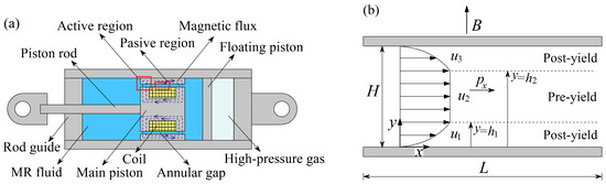
Figure 1. General sketch of (a) an MR valve and (b) the velocity profile in the active region.

2.2. Governing and Constitutive Equations

The flow field for an incompressible fluid is determined by the continuity and momentum conservation equations given by:

$$\nabla ·\mathbf{V}=0$$

(1)

and

$$\rho {\displaystyle \frac{D\mathbf{V}}{Dt}}=-\nabla p+\nabla ·\mathit{\tau },$$

(2)

where $\mathbf{V}$ is the velocity vector, $\rho$ is the fluid density, t is the time, p is the pressure, and $\mathit{\tau }$ is the stress tensor. Moreover, this study employs the Bingham model [18,19] to represent the non-Newtonian behavior of the MR fluid, as follows:

$$\mathit{\tau }={\tau }_0+{\eta }_p\dot{\gamma },$$

(3)

where ${\tau }_0$ is the yield stress, ${\eta }_p$ is the plastic viscosity, $\dot{\gamma }$ is the shear strain rate defined as $\dot{\gamma }=\left[(\nabla \mathbf{V})+{(\nabla \mathbf{V})}^{\mathbf{T}}\right]$, and ${(\nabla \mathbf{V})}^{\mathbf{T}}$ is the transpose of the tensor $(\nabla \mathbf{V})$. The liquid-type behavior of the MR fluid, represented by the post-yield regions in Figure 1b, establishes that the shear stress exceeds the yield stress. Therefore, the Bingham model reduces to the classic Newtonian model:

$$\mathit{\tau }={\eta }_p\dot{\gamma },$$

(4)

where ${\eta }_p$, which modifies the resistance to flow, determines the velocity magnitude of the liquid layers $u_1$ and $u_3$. On the other hand, the semi-solid behavior of the MR fluid, represented by the pre-yield region in Figure 1b, indicates that the shear stress applied in this area cannot deform the particle chain-like structure generated by the magnetic field. Therefore, the fluid layer in the pre-yield region does not deform $(\dot{\gamma }=0)$, and the Bingham model becomes:

$$\mathit{\tau }={\tau }_0,$$

(5)

where ${\tau }_0$ depends on the particle species and size, as well as the volume fraction of the MR fluid and strength of the applied magnetic field. In this regard, the saturation magnetization of magnetic particle species, $M_s$, plays a crucial role in the performance of MR fluids. For weak magnetic fields, the relationship between the magnetization of the MR fluid M and the magnetic field B is linear. As a result, the yield stress is as follows [8]:

$${\tau }_0=\varphi {\mu }_0{B}^2.$$

(6)

While for intermediate magnetic fields above the linear behavior and before particles are fully magnetized or saturated (saturation magnetization), the yield stress is as follows [3,8,37]:

$${\tau }_0=\sqrt{6}\varphi {\mu }_0{M}_s^{1/2}{B}^{3/2}$$

(7)

and, once a high magnetic field causes saturation magnetization of particles, the yield stress is field-independent and can be expressed as follows [3,6,8,37]:

$${\tau }_0=0.086\varphi {\mu }_0{M}_s^2.$$

(8)

Additionally, the competition between magnetostatic and hydrodynamic forces is essential in the formation and collapse of particle chain-like structures in MR fluids. Here, the magnetic attraction force between two particles generated by a magnetic field strength is [31,34]:

$$F_0={\displaystyle \frac{\pi }{48}}{\mu }_0{\sigma }^2{M}_p^2,$$

(9)

where $\sigma =2a$ is the diameter of spherical particles and $M_p=M/\varphi$ is the average magnetization of spherical particles. The magnetization of the MR fluid scales with the magnetic field as $M=B({\mu }_{eff}-1)/\varphi$, where ${\mu }_{eff}={\mu }_{cr}[1-3{\varphi }_{m}log(1-\varphi /{\varphi }_m)]$ is the effective permeability of the MR fluid, and ${\varphi }_m$ is the field-independent maximum packing fraction [2,38]. In this work, the maximum packing fraction is ${\varphi }_m=0.5236$ and indicates that the microstructures of monodispersed spherical particles are periodically arranged in single particle chains, resulting in a perfect three-dimensional cubic lattice [38,39]. On the other hand, magnetic particles experience viscous drag due to the carrier fluid motion caused by the pressure difference between the inlet and outlet of the valve; this drag force, also known as hydrodynamic force or viscous force, is defined as [28]:

$$F_H=3\pi {\eta }_c{\sigma }^2{\dot{\gamma }}_c,$$

(10)

where ${\eta }_c$ is the viscosity of the carrier fluid and ${\dot{\gamma }}_c$ is the characteristic shear rate of the system. In this context, the Mason number is the ratio of magnetostatic forces to hydrodynamic forces and represents the microscopic behavior of MR fluids, as follows [28]:

$$M_n={\displaystyle \frac{F_H}{F_0}}={\displaystyle \frac{3\pi {\eta }_c{\dot{\gamma }}_c}{{\tau }^{*}}},$$

(11)

where ${\tau }^{*}=F_0/{\sigma }^2$ is the magnetic stress.

2.3. Simplified Mathematical Model

The following assumptions, based on the channel geometry of the annular gap, the flow field conditions in the active region, and the constant piston movement, are taken into account to simplify the mathematical model [21,23,24]:

• The flow is steady, laminar, and fully developed.
• The flow is unidirectional on the x-axis.
• The annular gap is small relative to the annular radius.
• The pressure gradient $p_x$ is constant on the x-axis.
• The flow field neglects gravitational effects.

Therefore, the governing and constitutive equations given by (1)–(3) can be simplified in Cartesian coordinates as follows:

$${\displaystyle \frac{d{\tau }_{xy}}{dy}}=p_x,$$

(12)

where ${\tau }_{xy}$ is the shear stress, $p_x=\Delta p/L$ is the pressure gradient, and $\Delta p$ is the pressure drop generated by the pressure difference between the inlet and outlet of the MR valve. Furthermore, the following cases show the shear stress as a function of velocity gradient for each layer of the velocity profile in Figure 1b:

$$\begin{array}{cc}\hfill & \mathrm{Case} 1: \mathrm{For} \mathrm{the} \mathrm{liquid} \mathrm{layer} \mathrm{with} \mathrm{velocity}{u}_1\left({\displaystyle \frac{d{u}_1}{dy}}>0\right);{\tau }_{xy}={\eta }_p{\displaystyle \frac{d{u}_1}{dy}}.\hfill \\ \hfill & \mathrm{Case} 2: \mathrm{For} \mathrm{the} \mathrm{solid} \mathrm{layer} \mathrm{with} \mathrm{velocity}{u}_2\left({\displaystyle \frac{d{u}_2}{dy}}=0\right);{\tau }_{xy}={\tau }_0.\hfill \\ \hfill & \mathrm{Case} 3: \mathrm{For} \mathrm{the} \mathrm{liquid} \mathrm{layer} \mathrm{with} \mathrm{velocity}{u}_3\left({\displaystyle \frac{d{u}_3}{dy}}<0\right);{\tau }_{xy}={\eta }_p{\displaystyle \frac{d{u}_3}{dy}}.\hfill \end{array}$$

(13)

2.4. Boundary Conditions

The mathematical model requires boundary conditions at the interfaces to determine the flow field. In this sense, the hydrodynamic behavior of liquid layers (the post-yield regions in Figure 1b) assumes the no-slip boundary condition at the channel walls:

$$u_1=0\mathrm{at}y=0$$

(14)

and

$$u_3=0\mathrm{at}y=H.$$

(15)

Furthermore, the velocity of liquid layers at the interfaces $y=h_1$ and $y=h_2$ is equal to the plug flow velocity (the pre-yield region in Figure 1b), resulting in the velocity continuity conditions as:

$$u_1=u_2\mathrm{at}y=h_1$$

(16)

and

$$u_3=u_2\mathrm{at}y=h_2.$$

(17)

At the same time, at the interfaces $y=h_1$ and $y=h_2$, interactions between liquid and solid layers, consider the stress balance conditions as:

$${\tau }_0+{\left.{\eta }_p{\displaystyle \frac{d{u}_1}{dy}}\right|}_{y=h_1}={\tau }_0+{\left.{\eta }_p{\displaystyle \frac{d{u}_2}{dy}}\right|}_{y=h_1}$$

(18)

and

$${\tau }_0+{\left.{\eta }_p{\displaystyle \frac{d{u}_3}{dy}}\right|}_{y=h_2}={\tau }_0+{\left.{\eta }_p{\displaystyle \frac{d{u}_2}{dy}}\right|}_{y=h_2}.$$

(19)

However, the flow condition of the pre-yield region, which indicates that the velocity gradient of plug flow is zero ($d{u}_2/dy=0$ at $h_1\le y\le h_2$), simplifies Equations (18) and (19) as follows:

$${\left.{\displaystyle \frac{d{u}_1}{dy}}\right|}_{y=h_1}=0$$

(20)

and

$${\left.{\displaystyle \frac{d{u}_3}{dy}}\right|}_{y=h_2}=0.$$

(21)

3. Dimensionless Mathematical Model

This work employs the following dimensionless variables to normalize the mathematical model:

$$\overline{y}={\displaystyle \frac{y}{H}},\overline{u}={\displaystyle \frac{u}{u_c}},{\overline{\tau }}_{xy}={\displaystyle \frac{{\tau }_{xy}}{{\tau }_c}},$$

(22)

where $u_c=A_p{V}_p/A_v$ is the characteristic velocity, which represents the average fluid velocity in the valve gap [22,23], and ${\tau }_c={\eta }_p{\dot{\gamma }}_c$ is the characteristic stress [2,28]. Here, $A_p$ is the piston head area, $V_p$ is the piston velocity, $A_v=Hb$ is the flow path area in the MR valve, b is the channel width, and the flow field assumes the characteristic shear rate as ${\dot{\gamma }}_c\sim (u_c/H)$. Substituting Equation (22) into (12) and (13) gives the following. First, the dimensionless momentum equation becomes:

$${\displaystyle \frac{d{\overline{\tau }}_{xy}}{d\overline{y}}}=\Gamma ,$$

(23)

where $\Gamma =p_{x}H/{\tau }_c$ is the dimensionless pressure gradient. Second, the dimensionless shear stresses for the post-yield regions are:

$$\mathrm{for} \mathrm{the} \mathrm{liquid} \mathrm{layer} \mathrm{with} \mathrm{velocity}{\overline{u}}_1;{\overline{\tau }}_{xy}=\left({\displaystyle \frac{d{\overline{u}}_1}{d\overline{y}}}\right)$$

(24)

and

$$\mathrm{for} \mathrm{the} \mathrm{liquid} \mathrm{layer} \mathrm{with} \mathrm{velocity}{\overline{u}}_3;{\overline{\tau }}_{xy}=\left({\displaystyle \frac{d{\overline{u}}_3}{d\overline{y}}}\right).$$

(25)

And third, the dimensionless shear stress for the pre-yield region is determined by the Bingham number $Bi$, which establishes the ratio of the magnetic stress to the viscous stress at the macroscopic level:

$$\mathrm{for} \mathrm{the} \mathrm{solid} \mathrm{layer} \mathrm{with} \mathrm{velocity}{\overline{u}}_2;{\overline{\tau }}_{xy}=Bi={\displaystyle \frac{{\tau }_0}{{\eta }_p{\dot{\gamma }}_c}},$$

(26)

in addition, assuming that the characteristic shear rate ${\dot{\gamma }}_c$ is the same in both $Bi$ and $M_n$ [28], Equation (26) with the help of Equation (11) results in:

$$\mathrm{for} \mathrm{the} \mathrm{solid} \mathrm{layer} \mathrm{with} \mathrm{velocity}{\overline{u}}_2;{\overline{\tau }}_{xy}=Bi={\displaystyle \frac{3\pi {\overline{\tau }}_0{M}_n^{-1}}{\overline{\eta }}},$$

(27)

where ${\overline{\tau }}_0={\tau }_0/{\tau }^{*}$ is the dimensionless yield stress, which represents how effective the magnetic attraction between particles manifests as a yield stress [28]. In Equation (27), the Mason number incorporates the microscopic behavior of the MR fluid to determine the competition between viscous and magnetic stresses. Furthermore, $\overline{\eta }={\eta }_p/{\eta }_c$ represents the viscosity ratio of the MR fluid to the carrier fluid, thereby manifesting the effect of the addition of hard spherical particles to the Newtonian carrier fluid, as follows [2,39]:

$$\overline{\eta }={\displaystyle \frac{{\eta }_p}{{\eta }_c}}={\left(1-{\displaystyle \frac{\varphi }{{\varphi }_m}}\right)}^{-2.5{\varphi }_m},$$

(28)

where $\overline{\eta }>1$ represents the fluid viscosity dependent on the concentration of magnetic particles; $\overline{\eta }$ rises as $\varphi$ increases. Meanwhile, $\overline{\eta }=1$ recovers the initial viscosity of the Newtonian carrier fluid, indicating the absence of magnetic particles (${\eta }_p={\eta }_c$ in this case). Hence, substituting Equation (28) into (27) gives:

$$\mathrm{for} \mathrm{the} \mathrm{solid} \mathrm{layer} \mathrm{with} \mathrm{velocity}{\overline{u}}_2;{\overline{\tau }}_{xy}=Bi={\displaystyle \frac{3\pi {\overline{\tau }}_0{M}_n^{-1}}{{\left(1-\frac{\varphi }{{\varphi }_m}\right)}^{-2.5{\varphi }_m}}}.$$

(29)

On the other hand, the dimensionless boundary conditions to solve the flow field, by substituting Equation (22) into (14)–(17), (20) and (21), are the no-slip conditions at the walls:

$${\overline{u}}_1=0\mathrm{at}\overline{y}=0$$

(30)

and

$${\overline{u}}_3=0\mathrm{at}\overline{y}=1.$$

(31)

At the interfaces $\overline{y}={\overline{h}}_1$ and $\overline{y}={\overline{h}}_2$, the velocity continuity conditions are:

$${\overline{u}}_1={\overline{u}}_2\mathrm{at}\overline{y}={\overline{h}}_1$$

(32)

and

$${\overline{u}}_3={\overline{u}}_2\mathrm{at}\overline{y}={\overline{h}}_2,$$

(33)

while the stress balance conditions are:

$${\left.{\displaystyle \frac{d{\overline{u}}_1}{d\overline{y}}}\right|}_{\overline{y}={\overline{h}}_1}=0$$

(34)

and

$${\left.{\displaystyle \frac{d{\overline{u}}_3}{d\overline{y}}}\right|}_{\overline{y}={\overline{h}}_2}=0,$$

(35)

where ${\overline{h}}_1=h_1/H$ and ${\overline{h}}_2=h_2/H$ are the dimensionless interface positions that indicate the separation between liquid and solid layers.

4. Solution Methodology

4.1. Post-Yield Regions

The following procedures outline the solution methodology to determine the flow field for the liquid layers in Figure 1b. In this context, the momentum equations for the velocity components ${\overline{u}}_1$ and ${\overline{u}}_3$, by substituting Equations (24) and (25) into (23), are:

$${\displaystyle \frac{d}{d\overline{y}}}\left({\displaystyle \frac{d{\overline{u}}_1}{d\overline{y}}}\right)=\Gamma$$

(36)

and

$${\displaystyle \frac{d}{d\overline{y}}}\left({\displaystyle \frac{d{\overline{u}}_3}{d\overline{y}}}\right)=\Gamma .$$

(37)

Then, integrating Equations (36) and (37) once regarding the transverse coordinate $\overline{y}$ gives the velocity gradients for ${\overline{u}}_1$ and ${\overline{u}}_3$ as:

$${\displaystyle \frac{d{\overline{u}}_1}{d\overline{y}}}=-\Gamma (C_1-\overline{y})$$

(38)

and

$${\displaystyle \frac{d{\overline{u}}_3}{d\overline{y}}}=\Gamma (\overline{y}-C_2),$$

(39)

where $C_1$ and $C_2$ are integration constants. In this case, $C_1={\overline{h}}_1$ and $C_2={\overline{h}}_2$ when applying the stress balance conditions of Equations (34) and (35) to (38) and (39). Hence, Equations (38) and (39) become:

$${\displaystyle \frac{d{\overline{u}}_1}{d\overline{y}}}=-\Gamma ({\overline{h}}_1-\overline{y})$$

(40)

and

$${\displaystyle \frac{d{\overline{u}}_3}{d\overline{y}}}=\Gamma (\overline{y}-{\overline{h}}_2).$$

(41)

Meanwhile, integrating Equations (40) and (41) regarding the transverse coordinate $\overline{y}$ results in the velocity profiles for ${\overline{u}}_1$ and ${\overline{u}}_3$ as:

$${\overline{u}}_1={\displaystyle \frac{\Gamma }{2}}{({\overline{h}}_1-\overline{y})}^2+C_3$$

(42)

and

$${\overline{u}}_3={\displaystyle \frac{\Gamma }{2}}{(\overline{y}-{\overline{h}}_2)}^2+C_4,$$

(43)

where $C_3$ and $C_4$ are integration constants. Here, $C_3=C_4={\overline{u}}_2$ when applying the velocity continuity conditions of Equations (32) and (33) to (42) and (43). Therefore, the velocity profiles in Equations (42) and (43) depend on ${\overline{u}}_2$ as follows:

$${\overline{u}}_1={\displaystyle \frac{\Gamma }{2}}{({\overline{h}}_1-\overline{y})}^2+{\overline{u}}_2$$

(44)

and

$${\overline{u}}_3={\displaystyle \frac{\Gamma }{2}}{(\overline{y}-{\overline{h}}_2)}^2+{\overline{u}}_2.$$

(45)

Finally, substituting the no-slip conditions of Equations (30) and (31) into (44) and (45), two expressions for the velocity ${\overline{u}}_2$ result as:

$${\overline{u}}_2=-{\displaystyle \frac{\Gamma }{2}}{\overline{h}}_1^2$$

(46)

and

$${\overline{u}}_2=-{\displaystyle \frac{\Gamma }{2}}{(1-{\overline{h}}_2)}^2.$$

(47)

In particular, the relationship between interfaces ${\overline{h}}_1=1-{\overline{h}}_2$ is obtained by equating Equations (46) and (47). Also, the velocity profiles in Equations (44) and (45) depend on the interfaces ${\overline{h}}_1$ and ${\overline{h}}_2$, which establish the pre-yield thickness. Without a magnetic field strength, there is no solid region, and the interfaces ${\overline{h}}_1$ and ${\overline{h}}_2$ will indicate the maximum velocity position at $\overline{y}=0.5$. On the contrary, the interfaces ${\overline{h}}_1$ and ${\overline{h}}_2$ will have different positions when a magnetic field is applied.

4.2. Pre-Yield Region

The pre-yield region, defined by the interfaces ${\overline{h}}_1$ and ${\overline{h}}_2$, represents the semi-solid condition of the MR fluid and depends on the magnetic field intensity. The pre-yield thickness results from integrating Equation (23) in the range of ${\overline{h}}_1\le \overline{y}\le {\overline{h}}_2$, considering that the shear stresses at ${\overline{h}}_1$ and ${\overline{h}}_2$ are ${\overline{\tau }}_{xy}$ and $-{\overline{\tau }}_{xy}$, as follows [21,22,24]:

$${\int }_{{\overline{\tau }}_{xy}}^{-{\overline{\tau }}_{xy}}d{\overline{\tau }}_{xy}=\Gamma {\int }_{{\overline{h}}_1}^{{\overline{h}}_2}\overline{y}$$

(48)

and solving the definite integrals of Equation (48):

$$\overline{\delta }=-{\displaystyle \frac{2{\overline{\tau }}_{xy}}{\Gamma }},$$

(49)

where $\overline{\delta }={\overline{h}}_2-{\overline{h}}_1$ is the dimensionless pre-yield thickness. Then, substituting the shear stress of the pre-yield region of Equation (29) into (49) gives:

$$\overline{\delta }=-{\displaystyle \frac{2Bi}{\Gamma }}=-{\displaystyle \frac{6\pi {\overline{\tau }}_0{M}_n^{-1}}{{\left(1-\frac{\varphi }{{\varphi }_m}\right)}^{-2.5{\varphi }_m}\Gamma }}.$$

(50)

In particular, the interface positions ${\overline{h}}_1$ and ${\overline{h}}_2$ are calculated from Equation (50), considering the relationship between interfaces ${\overline{h}}_1=1-{\overline{h}}_2$ obtained by equating Equations (46) and (47). As a result, ${\overline{h}}_1$ and ${\overline{h}}_2$ are:

$${\overline{h}}_1={\displaystyle \frac{1}{2}}+{\displaystyle \frac{Bi}{\Gamma }}$$

(51)

and

$${\overline{h}}_2={\displaystyle \frac{1}{2}}-{\displaystyle \frac{Bi}{\Gamma }}.$$

(52)

4.3. Flow Rate

The sum of the fluid volume in each layer of the velocity profile in Figure 1b determines the total flow rate through the control valve [22,23,24]:

$$\begin{array}{cc}\hfill {\overline{Q}}_{T,x}=& {\displaystyle \frac{Q_{T,x}}{Q_c}}={\displaystyle \frac{b}{Q_c}}\left[{\int }_0^{h_1}{u}_{1}dy+{\int }_{h_1}^{h_2}{u}_{2}dy+{\int }_{h_2}^1{u}_{3}dy\right]\hfill \\ \hfill =& {\int }_0^{{\overline{h}}_1}{\overline{u}}_{1}d\overline{y}+{\int }_{{\overline{h}}_1}^{{\overline{h}}_2}{\overline{u}}_{2}d\overline{y}+{\int }_{{\overline{h}}_2}^1{\overline{u}}_{3}d\overline{y},\hfill \end{array}$$

(53)

where ${\overline{Q}}_{T,x}$ is the dimensionless flow rate on the x-axis, assuming that $Q_{T,x}$ is the flow rate on the x-axis and $Q_c=u_c{A}_v$ is the characteristic flow rate. Solving Equation (53) with the help of Equations (44)–(46):

$${\overline{Q}}_{T,x}={\displaystyle \frac{\Gamma }{6}}{\overline{h}}_1^3+{\displaystyle \frac{\Gamma }{6}}{(1-{\overline{h}}_2)}^3-{\displaystyle \frac{\Gamma }{2}}{\overline{h}}_1^2$$

(54)

and considering that ${\overline{h}}_1=1-{\overline{h}}_2$ (by equating Equations (46) and (47)) and ${\overline{h}}_1=(1/2)+(Bi/\Gamma )$ (see Equation (51)), Equation (54) is simplified to:

$${\overline{Q}}_{T,x}={\displaystyle \frac{\Gamma }{3}}{\left({\displaystyle \frac{1}{2}}+{\displaystyle \frac{Bi}{\Gamma }}\right)}^3-{\displaystyle \frac{\Gamma }{2}}{\left({\displaystyle \frac{1}{2}}+{\displaystyle \frac{Bi}{\Gamma }}\right)}^2.$$

(55)

4.4. Damping

The damping capacity of the MR damper is determined by equating the total flow rate generated by the control valve with the liquid volume displaced by the piston movement:

$${\overline{Q}}_{T,x}={\overline{Q}}_p={\overline{A}}_p{\overline{V}}_p,$$

(56)

where ${\overline{Q}}_p=Q_p/Q_c$ is the dimensionless flow rate produced by the piston movement, ${\overline{A}}_p=A_p/A_v$ is the dimensionless piston head area, ${\overline{V}}_p=V_p/u_c$ is the dimensionless piston velocity, and $V_p$ is the piston velocity. Thus, combining Equations (55) and (56) results in:

$${\overline{A}}_p{\overline{V}}_p={\displaystyle \frac{\Gamma }{3}}{\left({\displaystyle \frac{1}{2}}+{\displaystyle \frac{Bi}{\Gamma }}\right)}^3-{\displaystyle \frac{\Gamma }{2}}{\left({\displaystyle \frac{1}{2}}+{\displaystyle \frac{Bi}{\Gamma }}\right)}^2.$$

(57)

Regarding the dimensionless pressure gradient $\Gamma =p_{x}H/{\tau }_c$ in Equation (57), the pressure gradient $p_x$ on the x-axis generated by the pressure difference between the inlet and outlet of the MR valve is:

$$p_x={\displaystyle \frac{\Delta p}{L}}={\displaystyle \frac{F}{A_{p}L}},$$

(58)

where F is the damper force of the MR valve. Then, considering the force F as a linear damping force proportional to the piston velocity, $F=C_{eq}{V}_p$ [22,40], Equation (58) becomes:

$$p_x={\displaystyle \frac{C_{eq}{V}_p}{A_{p}L}},$$

(59)

where $C_{eq}$ is the equivalent viscous damping. As a result, the dimensionless pressure gradient $\Gamma$ with the help of Equation (59) gives:

$$\Gamma ={\displaystyle \frac{p_{x}H}{{\tau }_c}}={\displaystyle \frac{{\overline{C}}_{eq}{\overline{V}}_p}{{\overline{A}}_p}},$$

(60)

where ${\overline{C}}_{eq}=C_{eq}H/\left(L{\eta }_{p}b\right)$ is the dimensionless equivalent viscous damping. Therefore, substituting Equation (60) into (57) results in:

$${\overline{A}}_p{\overline{V}}_p={\displaystyle \frac{{\overline{C}}_{eq}{\overline{V}}_p/{\overline{A}}_p}{3}}{\left({\displaystyle \frac{1}{2}}+{\displaystyle \frac{Bi}{{\overline{C}}_{eq}{\overline{V}}_p/{\overline{A}}_p}}\right)}^3-{\displaystyle \frac{{\overline{C}}_{eq}{\overline{V}}_p/{\overline{A}}_p}{2}}{\left({\displaystyle \frac{1}{2}}+{\displaystyle \frac{Bi}{{\overline{C}}_{eq}{\overline{V}}_p/{\overline{A}}_p}}\right)}^2,$$

(61)

where ${\overline{C}}_{eq}$ represents the field-dependent damping by assuming that $Bi>0$, and it is determined by the following process. First, Equation (61) is rewritten algebraically as a third-degree polynomial:

$${\overline{C}}_{eq}^3{\left({\displaystyle \frac{{\overline{V}}_p}{{\overline{A}}_p}}\right)}^3+3{\overline{C}}_{eq}^2\left(Bi+4{\overline{A}}_p{\overline{V}}_p\right){\left({\displaystyle \frac{{\overline{V}}_p}{{\overline{A}}_p}}\right)}^2-4B{i}^3=0$$

(62)

and second, by applying the Cardan–Tartaglia method for a cubic equation, ${\overline{C}}_{eq}$ in Equation (62) is:

$${\overline{C}}_{eq}=\sqrt[3]{-{\displaystyle \frac{b_1}{2}}+\sqrt{{\displaystyle \frac{b_1^2}{4}}+{\displaystyle \frac{b_2^3}{27}}}}+\sqrt[3]{-{\displaystyle \frac{b_1}{2}}-\sqrt{{\displaystyle \frac{b_1^2}{4}}+{\displaystyle \frac{b_2^3}{27}}}}-{\displaystyle \frac{a_1}{3}},$$

(63)

where

$$\begin{array}{cc}\hfill & b_1=a_2+{\displaystyle \frac{2a_1^3}{27}},b_2=-{\displaystyle \frac{a_1^2}{3}},a_1={\displaystyle \frac{X_2}{X_1}},a_2={\displaystyle \frac{X_3}{X_1}},X_1={\left({\displaystyle \frac{{\overline{V}}_p}{{\overline{A}}_p}}\right)}^3,\hfill \\ \hfill & X_2=3\left(Bi+4{\overline{A}}_p{\overline{V}}_p\right){\left({\displaystyle \frac{{\overline{V}}_p}{{\overline{A}}_p}}\right)}^2,X_3=-4B{i}^3.\hfill \end{array}$$

(64)

On the other hand, when there is no magnetic field strength on the MR fluid, ${\overline{C}}_{eq}$ becomes ${\overline{C}}_{off}$, and Equation (61) evaluated with $Bi=0$ results in:

$$0={\displaystyle \frac{{\overline{C}}_{off}}{12}}\left({\displaystyle \frac{{\overline{V}}_p}{{\overline{A}}_p}}\right)+{\overline{A}}_p{\overline{V}}_p,$$

(65)

where ${\overline{C}}_{off}=C_{off}H/\left(L{\eta }_{p}b\right)$ is the dimensionless Newtonian viscous damping with $C_{off}$ as the Newtonian viscous damping. In this case, ${\overline{C}}_{off}$ in Equation (65) is as follows:

$${\overline{C}}_{off}=-12{\overline{A}}_p^2.$$

(66)

Finally, the damping coefficient ${\overline{C}}_r$ is the ratio of the field-dependent damping to the Newtonian viscous damping and represents the damping capacity of the MR damper:

$${\overline{C}}_r={\displaystyle \frac{{\overline{C}}_{eq}}{{\overline{C}}_{off}}}.$$

(67)

5. Results and Discussion

For this analysis of results, the following parameter ranges establish the corresponding values of the dimensionless parameters: $0.2\le \varphi \le 0.3$, ${\varphi }_m=0.5236$, $0.01\le {\eta }_c\le 0.5$ Pa s, ${\mu }_0=4\pi \times {10}^{-7}$ T m A⁻¹, ${\mu }_{cr}=1$, $0\le B\le 1600$ kA m⁻¹, $475\le M_s\le 1600$ kA m⁻¹, and $0\le {\dot{\gamma }}_c\le$ 12,000 s⁻¹ [2,27,28,31,38,41]. The MR valve assumes the following geometry and piston velocity: $7\times {10}^{-4}\le A_p\le 0.002$ m², $8\times {10}^{-4}\le H\le 0.022$ m, $0.08\le b\le 0.15$ m, $0.01\le L\le 0.05$ m, and $0\le V_p\le 0.5$ m s⁻¹ [21,22,23,24,42].

5.1. Validation

To validate the results of this investigation, Figure 2 shows a comparison between the velocity profiles of this work using Equations (44)–(46) and the following velocity profiles extracted from the work developed by Wereley [22]:

$${\overline{u}}_1={\left(1-\overline{\delta }\right)}^2-{\left(-2\overline{y}-\overline{\delta }\right)}^2,$$

(68)

$${\overline{u}}_2={\left(1-\overline{\delta }\right)}^2$$

(69)

and

$${\overline{u}}_3={\left(1-\overline{\delta }\right)}^2-{\left(2\overline{y}-\overline{\delta }\right)}^2,$$

(70)

where Equations (68)–(70) describe the hydrodynamic behavior of an MR valve through the Bingham model. In this context, to recover the results obtained by Wereley [22] regarding the dimensionless pre-yield thickness ($\overline{\delta }=0.6$, $0.3$, and 0), Equations (44)–(46) use the following values: $\Gamma =-8$, and $Bi=2.4, 1.2, 0$ to obtain ${\overline{h}}_1=0.2, 0.35, 0.5$ and ${\overline{h}}_2=0.8, 0.65, 0.5$. The results in Figure 2 present the competition between the fluid resistance through the parameter $\overline{\delta }={\overline{h}}_2-{\overline{h}}_1$ and the shear stress due to the pressure gradient generated by the piston movement. The magnetic field effect increases the pre-yield thickness and reduces the flow velocity, reaching the lowest velocity when $\overline{\delta }=0.6$. Meanwhile, the absence of magnetic field strength, which is indicated by $\overline{\delta }=0$, results in the total deformation of the MR fluid (here, the fluid volume is purely liquid). In all cases, the velocity profiles of both works overlap, indicating the good performance and convergence of the solution achieved by this research. The pre-yield thicknesses $\overline{\delta }=0.6$, $0.3$, and 0, obtained from the work of Wereley [22], do not provide information on fluid properties, magnetic field strength, or pressure gradient. Therefore, this is a clear difference concerning the present work, which aims to analyze the valve behavior considering the microstructural characteristics of the MR fluid.

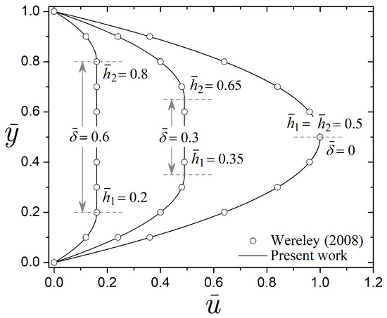
Figure 2. Dimensionless velocity profiles for different values of the pre-yield thickness from the present work and the research reported by Wereley [22].

5.2. Criteria for Estimating Dimensionless Parameters

Magnetic particles dispersed in the carrier fluid control the properties of the MR fluid in Figure 3. This figure illustrates the effect of adding hard spherical particles to the carrier fluid on the viscosity ratio and effective permeability of the MR fluid, considering the range of $0.2\le \varphi \le 0.3$ for typical MR damper applications. It is important to consider that, for high particle concentrations above $\varphi =0.3$, the MR fluid can acquire the behavior of a solid paste, complicating fluid manipulation [2]. Conversely, in the absence of magnetic particles $\varphi =0$, the MR fluid recovers the viscosity of the carrier fluid ${\eta }_p={\eta }_c$ according to Equation (28). Thus, in Figure 3, the field-independent viscosity of the MR fluid increases by incorporating particles into the carrier fluid, reaching the highest viscosity of $\overline{\eta }=3.04$ when $\varphi =0.3$. Furthermore, the MR fluid obtains viscosities of ${\eta }_p=0.93$ and $1.52$ Pa s when $\varphi =0.2$ and $0.3$, considering a particular carrier fluid viscosity of ${\eta }_c=0.5$ Pa s (silicone oil) [27]. This increase in $\varphi$ represents an increase in viscosity of the MR fluid of $86\%$ when $\varphi =0.2$ and $204\%$ when $\varphi =0.3$ compared to the initial viscosity of ${\eta }_c=0.5$ Pa s. In this context, the results in Figure 3 enable the evaluation of the Mason number or the Bingham number, assuming that the increase in viscosity contributes to the hydrodynamic stress. On the other hand, in the inset of Figure 3, the particle volume fraction $\varphi$ also modifies the effective permeability of the MR fluid (${\mu }_{eff}={\mu }_{cr}[1-3{\varphi }_{m}log(1-\varphi /{\varphi }_m)]$ in Section 2.2), taking as a reference that ${\mu }_{cr}=1$ [31,38]. According to the previous equation, the parameter $\varphi$ provides the magnetic characteristics of the MR fluid, considering that the carrier fluid is non-magnetic; ${\mu }_{eff}={\mu }_{cr}=1$ when $\varphi =0$, while ${\mu }_{eff}=1.62$ and $2.1$ when $\varphi =0.2$ and $0.3$, respectively. Therefore, because the effective permeability is associated with the magnetization of the MR fluid, the fluid exhibits greater magnetic susceptibility as particle concentration increases, resulting in more significant magnetic stress (see Section 2.2). Also, the increase in magnetic particles modifies the capacity of the MR fluid to form chain-like structures when a magnetic field is applied, affecting the damping force that regulates flow through the valve.

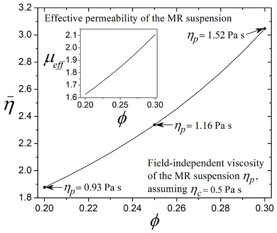
Figure 3. Dimensionless viscosity $\overline{\eta }$ and effective permeability ${\mu }_{eff}$ of the MR fluid for different values of the particle volume fraction $\varphi$.

Another aspect to consider is that the MR fluid subjected to a magnetic field acquires the behavior of a semi-solid with a certain yield stress. This fluid condition is due to the alignment of particles in the direction of the magnetic field, resulting in chain-like structures that inhibit fluid motion. Figure 4 estimates the dimensionless yield stress ${\overline{\tau }}_0={\tau }_0/{\tau }^{*}$ for different particle volume fractions $\varphi$ and magnetic fields B, considering hard spherical particles ($0.76\pm 0.4$ μm) of iron with $M_s=1600$ kA m⁻¹ [41]. Here, the parameter ${\overline{\tau }}_0$ exhibits the ratio of the yield stress ${\tau }_0$ to the magnetic stress ${\tau }^{*}$ (magnetic attraction force between particles), comparing the reference mechanical resistance of the MR fluid at macro and micro scales [28]; see Section 3. For low magnetic fields, the magnetization of the MR fluid is proportional to $B^2$ (see Equation (6)). Carlson and Jolly [11] report that MR fluids exhibit approximately linear magnetic properties up to an applied field of about $B=0.02/{\mu }_0\approx 16$ kA m⁻¹ in this regime, while for intermediate magnetic fields, the magnetization of the MR fluid scales nonlinearly with $B^{3/2}$ (see Equation (7)). Finally, for high magnetic fields sufficient to achieve the saturation point, the yield stress is field-independent and proportional to $M_s^2$ (see Equation (8)). In Figure 4, the magnetic stress (${\tau }^{*}=F_0/{\sigma }^2=\pi {\mu }_0{M}_p^2/48$) scales with the average magnetization of particles ($M_p=M/\varphi$), which is generally larger than the magnetization of the MR fluid ($M=B({\mu }_{eff}-1)/\varphi$). As a result, the magnetic stress exceeds the yield stress in all cases (${\tau }^{*}>{\tau }_0$), and thus ${\overline{\tau }}_0<1$. Moreover, the parameter ${\overline{\tau }}_0$ at a high magnetic field is lower than ${\overline{\tau }}_0$ at a low magnetic field due to the nonlinearity of the magnetization. Here, ${\overline{\tau }}_0=0.12$ and $0.41$ when $\varphi =0.2$ and $0.3$ with the low magnetic field ($B=16$ kA m⁻¹), while ${\overline{\tau }}_0=0.01$ and $0.03$ when $\varphi =0.2$ and $0.3$ with the high magnetic field ($M_s=1600$ kA m⁻¹). Therefore, these results demonstrate that increasing $\varphi$ from $0.2$ to $0.3$ (either for low, intermediate, and high magnetic fields) enhances the fluid resistance, assuming that the field-responsive effect of the MR fluid depends on the concentration of magnetic particles. Also, the most significant change in the dimensionless yield stress due to the increase in particle volume fraction occurs at the low magnetic field ($B=16$ kA m⁻¹).

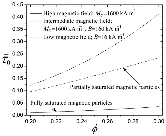
Figure 4. Dimensionless yield stress ${\overline{\mathit{\tau }}}_0$ for different values of the particle volume fraction $\varphi$.

In the evaluation of the dimensionless parameters in this work, it is clear that the magnetic field strength contributes to the formation of particle chain-like structures, thereby increasing the MR fluid resistance. Nevertheless, magnetic particles experience viscous drag due to the pressure drop across the control valve. In this context, the dimensionless Mason number $M_n$ determines the competition between magnetostatic and hydrodynamic forces at the microscopic level, which establishes the pre-yield thickness of the MR fluid. Figure 5a shows the Mason number (see Equation (11)) as a function of the magnetic stress ${\tau }^{*}=F_0/{\sigma }^2$ (see Equation (9)) for different values of the particle volume fraction $\varphi$ and three intermediate magnetic fields B, considering a carrier fluid viscosity of ${\eta }_c=0.5$ Pa s and a strain rate of ${\dot{\gamma }}_c$ = 12,000 s⁻¹ to estimate the hydrodynamic stress. In general, the Mason number decreases as the magnetic field magnifies the magnetic stress according to Equations (9) and (11), indicating that magnetic forces govern the microscopic behavior of the MR fluid. Meanwhile, the increase in magnetic particles reduces both the average magnetization of particles $M_p$ and the magnetic stress ${\tau }^{*}$, increasing the Mason number. It is important to establish that the equilibrium between magnetic and hydrodynamic forces occurs when $M_n=1$ [2]. Once the hydrodynamic forces equal or exceed the magnetic forces $(M_n\ge 1)$, the MR fluid acts as a purely liquid layer [2,32].

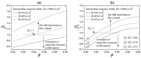
Figure 5. (a) Mason number $M_n$ and (b) critical Mason number $M_n^{*}$ for different values of the particle volume fraction $\varphi$.

On the other hand, assuming that the ratio of magnetic and viscous forces scales linearly from the microscopic to the macroscopic level, the Mason number is inversely related to the Bingham number. With the above, a relevant feature in the design of MR fluid-based devices is the critical Mason number $M_n^{*}=Bi{M}_n=3\pi {\overline{\tau }}_0/\overline{\eta }$, which determines the formation and collapse of particle chain-like structures [28]. Therefore, Figure 5b evaluates the critical Mason number from Figure 5a, which depends only on the dimensionless yield stress ${\overline{\tau }}_0$ and viscosity ratio $\overline{\eta }$. Typically, the critical Mason number follows the behavior of the Mason number, where $M_n^{*}$ increases as the magnetic field decreases and the particle volume fraction increases. The critical Mason number is constant and serves as a transition measure between the Mason number and the Bingham number $(Bi=M_n^{*}{M}_n^{-1})$. Above the critical Mason number $(M_n^{*}>1)$, the chain-like structures will not be able to form since the viscous drag on the MR particles prevents them from agglomerating together [2]. Usually, the critical Mason number is low; for high magnetic fields, the parameter $M_n^{*}$ is of the order of ${10}^{-2}$. Points $a1, a2, a3$, indicate $M_n^{*}=0.86, 0.78, 0.73$, respectively, and are selected for further analysis in Figure 6.

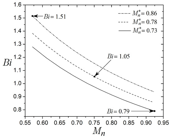
Figure 6. Bingham number $Bi$ for different values of the Mason number $M_n$ and the critical Mason number $M_n^{*}$.

Figure 6 evaluates the Bingham number $Bi$ as a function of the Mason number $M_n$ and three values of the critical Mason number $M_n^{*}$. Here, $M_n^{*}=0.73$, $0.78$, and $0.86$ are extracted from Figure 5b, considering points $a1$, $a2$, and $a3$. Meanwhile, the range of $0.57\le M_n\le 0.92$ is extracted from Figure 5a for the case of $B=70$ kA m⁻¹. To recover the range of $0.57\le M_n\le 0.92$ through the magnetic fields of $B=50$ and 60 kA m⁻¹, the strain rate ${\dot{\gamma }}_c$ in the Mason number calculation must be less than 12,000 s⁻¹. In this context, the limits of $M_n<1$ and $M_n^{*}<1$ ensure the formation of particle chain-like structures that result in the solid region of the MR fluid, which is essential to control flow through the valve. The dimensionless Bingham number establishes the ratio of magnetic stress to viscous stress and scales with $M_n^{-1}$.

The field-responsive effect of the MR fluid increases as the Bingham number rises, indicating that the magnetic field modifies its properties. This behavior implies that the microscopic characteristics of magnetic particles dispersed in the carrier fluid significantly influence the performance of the MR fluid. The critical Mason number $M_n^{*}$ is constant and manifests the changes in yield stress and viscosity due to the addition of magnetic particles in the carrier fluid. In this sense, the Bingham number increases in all cases in response to an increase in $M_n^{*}$. The results in this section show the MR fluid response to the magnetic field, which serves as a reference to estimate the dimensionless parameters required to analyze the control valve. These evaluations reveal the mechanical resistance of the MR fluid at the macroscopic level, considering its microscopic characteristics associated with the formation of chain-like structures that inhibit fluid motion. Points $Bi=0.79, 1.05, 1.51$ are selected for further analysis in Figure 7.

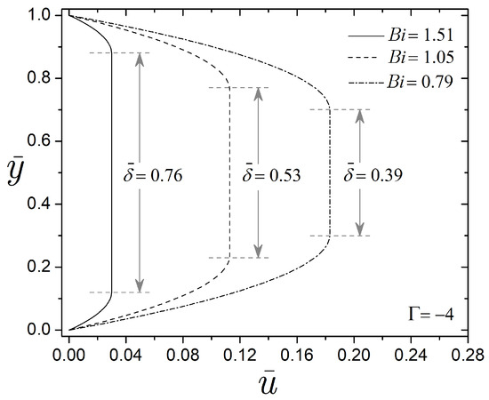
Figure 7. Dimensionless velocity profiles for different values of the Bingham number $Bi$.

5.3. Velocity Profiles and Flow Rates

This section presents the hydrodynamic behavior of the MR valve in terms of dimensionless parameters, considering the effects of intermediate and high magnetic fields on the MR fluid. This study seeks to highlight the qualities of the MR fluid in regulating flow through the control valve, assuming the nonlinearity of particle magnetization that depends on the magnetic field strength. Figure 7 shows the velocity profiles for $Bi=0.79$, $1.05$, and $1.51$ extracted from Figure 6. To simulate the performance of the MR fluid through the control valve, a pressure gradient of $\Gamma =-4$ drives the fluid volume from the rebound chamber to the compression chamber in Figure 1a. The negative sign indicates the flow on the positive x-axis, which occurs when the piston rod leaves the cylinder. The thicknesses of liquid and solid regions depend on the competition between the fluid resistance, as measured by the Bingham number, and the shear stress due to the pressure gradient. In the absence of a magnetic field strength ($Bi=0$), the MR fluid behaves as a completely liquid layer. On the contrary, increasing the Bingham number ($Bi>0$) reduces the thickness of liquid layers and generates a solid layer at the center of the channel. This solid layer represents the particle chain-like structures that are not broken. Here, the dimensionless pre-yield thickness is determined by Equation (50), resulting in $\overline{\delta }=0.76, 0.53,$ and $0.39$ for each value of $Bi=1.51, 1.05,$ and 0.79. The MR fluid can withstand a certain load before deforming. The maximum pressure gradient ${\Gamma }_{max}=-2Bi$ applied to the fluid before liquid regions appear is determined by Equation (50), considering $\overline{\delta }=1$ (completely solid layer) and assigning ${\Gamma }_{max}$ instead of $\Gamma$. Therefore, the valve remains closed in all cases when $\Gamma \le {\Gamma }_{max}$. Once $\Gamma$ exceeds ${\Gamma }_{max}$, the valve opens, as in Figure 7, where $\Gamma >{\Gamma }_{max}$ holds since $\Gamma =-4$ and ${\Gamma }_{max}=-1.58, -2.1, -3.02$ for $Bi=0.79, 1.05, 1.51$, respectively.

Figure 8 presents the velocity profiles as a function of the transverse coordinate $\overline{y}$ and different pressure gradients $\Gamma$, where the velocity profiles represent the flow field through the annular gap in the active region of the MR valve, and the pressure gradient results from the piston movement. This figure illustrates the hydrodynamic response of the MR fluid under two magnetic fields to regulate flow in the valve. In this context, the results are evaluated with $\varphi =0.2$, ${\eta }_c=0.5$ Pa s, $\dot{\gamma }=9000$ s⁻¹, and intermediate magnetic fields from Equation (7) with $M_s=1600$ kA m⁻¹. Furthermore, the velocity profiles exhibit a mechanical resistance (via the Bingham number) of $Bi=2.08$ for the lines with symbols and $Bi=3.83$ for the lines without symbols. Also, the magnetic stress is greater than the hydrodynamic stress in all cases of this figure, and thus $M_n^{*}<1$ and $M_n<1$. In the velocity profiles without symbols, the MR fluid withstands a compression force of ${\Gamma }_{max}=-7.66$. Therefore, the valve remains closed until the pressure gradient $\Gamma$ applied to the flow exceeds ${\Gamma }_{max}$, as in the equilibrium condition of the velocity profile without flow (solid line without symbols, where $\Gamma ={\Gamma }_{max}=-7.66$). Meanwhile, the valve opens when $\Gamma >{\Gamma }_{max}$, as for the dashed lines without symbols corresponding to $\Gamma =-10$ and $-13$, which lead to pre-yield thicknesses of $\overline{\delta }=0.76$ and $0.58$, respectively. On the other hand, decreasing the magnetic field from $B=120$ kA m⁻¹ to $B=80$ kA m⁻¹ reduces the fluid resistance from ${\Gamma }_{max}=-7.66$ to ${\Gamma }_{max}=-4.16$ in the velocity profiles with symbols. This result implies that the velocity profiles with symbols offer less resistance to deformation than those without symbols. The velocity profiles with symbols include certain liquid regions, considering that in all cases, $\Gamma >{\Gamma }_{max}$. Here, the pre-yield thicknesses are $\overline{\delta }=0.54$, $0.41$, and $0.32$ for $\Gamma =-7.66$, $-10$, and $-13$, respectively. When comparing the pre-yield thicknesses of the velocity profiles with and without symbols against the pre-yield thickness of the fully closed valve ($\overline{\delta }=1$), the reduction in the magnetic effect on the MR fluid from $B=120$ kA m⁻¹ to $B=80$ kA m⁻¹ leads to a valve opening of $0\%$ to $46\%$ when $\Gamma =-7.66$, $24\%$ to $59\%$ when $\Gamma =-10$, and $42\%$ to $68\%$ when $\Gamma =-13$. In this comparison, liquid regions establish the valve opening percentages.

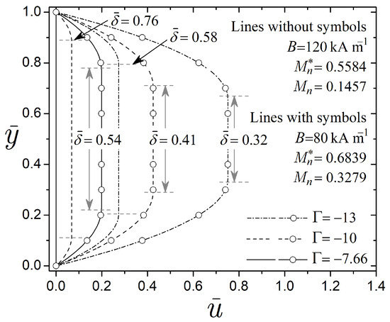
Figure 8. Dimensionless velocity profiles for different values of the pressure gradient $\Gamma$ and the magnetic field B.

Figure 9 illustrates the velocity profiles as a function of the transverse coordinate $\overline{y}$ and different values of the Mason number $M_n$ and the particle volume fraction $\varphi$. In this figure, the Mason number represents the formation and collapse of particle chain-like structures in the active region of the MR damper when a magnetic field is applied. Additionally, the Mason number analysis in the behavior of the valve also shows the competition between the fluid resistance that leads to the valve closing and the piston motion that opens the valve. The flow hydrodynamic assumes that magnetic particles, which are dispersed in a carrier fluid with viscosity ${\eta }_c=0.5$ Pa s, saturate at a high magnetic field. Hence, the yield stress ${\overline{\tau }}_0$ is calculated from Equation (8), considering a saturation magnetization of $M_s=1600$ kA m⁻¹. Meanwhile, a high strain rate of ${\dot{\gamma }}_c$ = 12,000 s⁻¹ on the MR fluid generates liquid regions in the flow field. The addition of hard spherical particles to the carrier fluid modifies the physical properties of the MR fluid; increasing $\varphi$ from $0.2$ to $0.3$ increases both the fluid viscosity $\overline{\eta }$ (see Figure 3) and the yield stress ${\overline{\tau }}_0$ (see Figure 4). In this sense, the critical Mason number $M_n^{*}=3\pi {\overline{\tau }}_0/\overline{\eta }$, which represents the influence of $\varphi$ on the carrier fluid, can capture the above behaviors. For a high and constant magnetic field, the flow field with $\varphi =0.2$ and $0.3$ results in $M_n^{*}=0.05$ and $0.1$, respectively. Furthermore, in this range of $0.05\le M_n^{*}\le 0.1$ with ${\eta }_c=0.5$ Pa s and ${\dot{\gamma }}_c$ = 12,000 s⁻¹, the Mason number $M_n$ varies from $0.01$ to $0.02$. Therefore, the mechanical resistance of the MR fluid (via the Bingham number $Bi$), by evaluating $M_n^{*}=0.05$ and $0.1$ with $M_n=0.01$, $0.015$, and $0.02$, is $Bi=10$, $6.66$, and 5 for $M_n=0.01$, $0.015$, and $0.02$ in the velocity profiles without symbols ($\varphi =0.3$ and $M_n^{*}=0.1$). Meanwhile, the values are $Bi=5$, $3.33$, and $2.5$ for $M_n=0.01$, $0.015$, and $0.02$ in the velocity profiles with symbols ($\varphi =0.2$ and $M_n^{*}=0.05$).

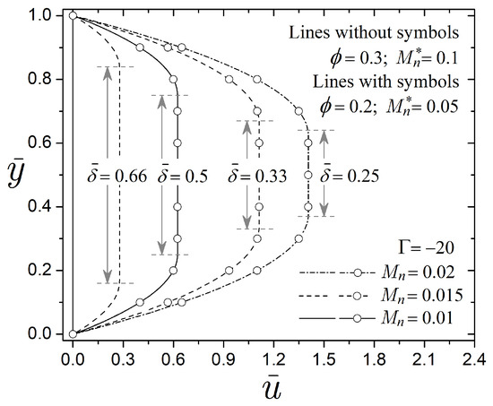
Figure 9. Dimensionless velocity profiles for different values of the particle volume fraction $\varphi$ and the Mason number $M_n$.

In Figure 9, the velocity profiles are evaluated with a pressure gradient of $\Gamma =-20$, taking as a reference ${\Gamma }_{max}=-2Bi=-20$, which arises from the combination of parameters that produces the highest resistance ($\varphi =0.3$, $M_n^{*}=0.1$, and $M_n=0.01$ to obtain $Bi=10$). As a result, the velocity profile corresponding to the solid line without symbols lacks liquid regions since $\Gamma ={\Gamma }_{max}$. Then, the increase in hydrodynamic stress (via the Mason number $M_n$) in the velocity profiles without symbols from $M_n=0.01$ to $0.015$ and $0.02$ reduces the pre-yield thickness from $\overline{\delta }=1$ to $0.66$ and $0.5$. Additionally, comparing the velocity profiles with and without symbols, the reduction in fluid resistance (via the particle volume fraction $\varphi$) from $\varphi =0.3$ to $0.2$ also reduces the pre-yield thickness from $\overline{\delta }=1$, $0.66$, and $0.5$ to $\overline{\delta }=0.5$, $0.33$, and $0.25$ when $M_n=0.01$, $0.015$, and $0.02$, respectively. In particular, the velocity profile with $\varphi =0.3$ and $M_n=0.02$ overlaps with the velocity profile with $\varphi =0.2$ and $M_n=0.01$, since both reach the same Bingham number ($Bi=5$). From these results, it is notable that the concentration of magnetic particles in the carrier fluid plays a crucial role in the performance of the MR valve, as increasing the particle volume fraction restricts flow through the valve.

On the other hand, Figure 10 exhibits the liquid transfer between the compression and rebound chambers in the MR damper for different pressure gradients generated by the piston motion. Figure 10a complements the results of Figure 8 by evaluating the dimensionless total flow rate ${\overline{Q}}_{T,x}$ from Equation (55), considering different pressure gradients $\Gamma$ on the flow field. The dimensionless parameters, such as $M_n^{*}=0.6839$, $M_n=0.3279$, $Bi=2.08$, and ${\Gamma }_{max}=-4.16$ for $B=80$ kA m⁻¹, as well as $M_n^{*}=0.5584$, $M_n=0.1457$, $Bi=3.83$, and ${\Gamma }_{max}=-7.66$ for $B=120$ kA m⁻¹, are extracted from Figure 8. Additionally, this figure extends the hydrodynamic analysis by incorporating the magnetic field of $B=160$ kA m⁻¹, which gives $M_n^{*}=0.4836$, $M_n=0.0819$, $Bi=5.89$, and ${\Gamma }_{max}=-11.79$. In the previous values, the parameter ${\Gamma }_{max}$ serves as a reference measure to estimate the pressure gradient required to open the MR valve, which occurs when $\Gamma$ exceeds ${\Gamma }_{max}$. According to Figure 10a, the increase in magnetic field strengthens the alignment of magnetic particles that inhibit fluid motion, thereby enhancing the mechanical resistance of the MR fluid. Therefore, the increase in magnetic field from $B=80$ to 160 kA m⁻¹ reduces the flow rate, leading to the valve closing. When $\Gamma =-10$, the magnetic fields $B=80$, 120, and 160 kA m⁻¹ produce flow rates of ${\overline{Q}}_{T,x}=0.34$, $0.06$, and 0, respectively. Meanwhile, when $\Gamma =-16$, the magnetic fields $B=80$, 120, and 160 kA m⁻¹ result in ${\overline{Q}}_{T,x}=0.82$, $0.45$, and $0.12$, respectively. In this comparison, $B=80$ kA m⁻¹ generates substantial flow rates in favor of the valve opening, increasing flow by $141\%$ when $\Gamma$ increases from $-10$ to $-16$, while $B=160$ kA m⁻¹ induces greater resistance to flow, thus generating lower flow rates than $B=80$ kA m⁻¹.

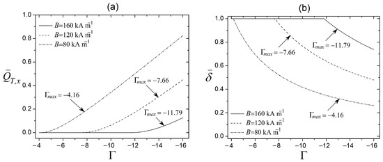
Figure 10. (a) Dimensionless flow rate ${\overline{Q}}_{T,x}$ and (b) dimensionless thickness of the solid region $\overline{\delta }$, both as a function of the pressure gradient $\Gamma$.

Complementary to Figure 10a, Figure 10b presents the dimensionless pre-yield thickness $\overline{\delta }$ for different pressure gradients $\Gamma$. In general, the magnetic field enhances the fluid resistance, resulting in thicker solid layers when B increases from 80 to 160 kA m⁻¹. Conversely, the increase in $\Gamma$ weakens the particle chain-like structure of the MR fluid, reducing the solid region. When $\Gamma$ increases from $-10$ to $-16$, the pre-yield thickness decreases from $\overline{\delta }=0.41$, $0.76$, and 1 to $\overline{\delta }=0.26$, $0.47$, and $0.73$ when $B=80$, 120, and 160 kA m⁻¹, respectively. These reductions in the solid region reflect an increase in the percentage of the valve opening of $59\%$ to $74\%$, $24\%$ to $53\%$, and $0\%$ to $27\%$ when $B=80$, 120, and 160 kA m⁻¹, respectively. Here, the percentage of liquid regions measures the valve opening, assuming that the valve is fully open with $\overline{\delta }=0$ ($100\%$) and fully closed with $\overline{\delta }=1$ ($0\%$). Therefore, the competition between the fluid resistance and the pressure gradient modifies the pre-yield thickness that inhibits fluid motion, thereby generating interesting behaviors in the valve hydrodynamics.

Figure 11 determines the dimensionless total flow rate ${\overline{Q}}_{T,x}$ as a function of the Mason number for a flow exposed to a high magnetic field, considering three different particle volume fractions $\varphi$ and two different pressure gradients $\Gamma$. The results show the influence of adding hard spherical particles into the carrier fluid on the hydrodynamic performance of the MR valve. The flow field assumes that magnetic particles dispersed in the carrier fluid saturate at a high magnetic field, considering a saturation magnetization of $M_s=1600$ kA m⁻¹. Therefore, the viscosity $\overline{\eta }$ and the yield stress ${\overline{\tau }}_0$ of the MR fluid are field-independent and depend only on the particle volume fraction $\varphi$; under these conditions, Equations (28) and (8) determine $\overline{\eta }$ and ${\overline{\tau }}_0$, then Equation (27) establishes the Bingham number $Bi$ in this figure. In this sense, $\overline{\eta }=1.8774$ and ${\overline{\tau }}_0=0.0105$ for $\varphi =0.2$, $\overline{\eta }=2.3387$ and ${\overline{\tau }}_0=0.0205$ for $\varphi =0.25$, and $\overline{\eta }=3.0458$ and ${\overline{\tau }}_0=0.0354$ for $\varphi =0.3$. Moreover, the driving force for pumping the MR fluid comes from a pressure gradient of $\Gamma =-15$ (lines without symbols) and $\Gamma =-45$ (lines with symbols). As a result, the Bingham numbers for the pressure gradient $\Gamma =-15$ are $Bi=10.97$ for $\varphi =0.3$, $Bi=8.27$ for $\varphi =0.25$, and $Bi=5.27$ for $\varphi =0.2$. Meanwhile, the Bingham numbers for the pressure gradient $\Gamma =-45$ are $Bi=2.19$ for $\varphi =0.3$, $Bi=1.65$ for $\varphi =0.25$, and $Bi=1.05$ for $\varphi =0.2$. In both results ($\Gamma =-15$ and $\Gamma =-45$), the flow rate ${\overline{Q}}_{T,x}$ decreases as the particle volume fraction $\varphi$ increases from $0.2$ to $0.3$, reflecting variations in the physical properties of the MR fluid. Also, increases in viscosity $\overline{\eta }$ and yield stress ${\overline{\tau }}_0$ reduce flow, as these parameters are associated with resistance to movement. In this context, the particle volume fraction $\varphi$ can regulate the flow through the control valve by modifying the flow characteristics of the MR fluid. On the other hand, the Mason number $M_n$, which indicates the ratio of viscous stress to magnetic stress, also affects the flow rate. For $\Gamma =-15$, the valve remains closed at $\overline{\delta }=1$, and flow arises as the Mason number increases, indicating an increase in viscous stress. Meanwhile, for $\Gamma =-45$, the highest flow rates occur at $\overline{\delta }\approx 0$ (when $\Gamma \gg Bi$), where the valve is fully open.

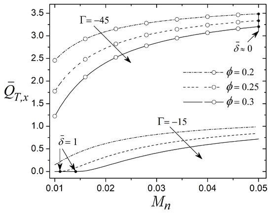
Figure 11. Dimensionless flow rate ${\overline{Q}}_{T,x}$ as a function of the Mason number and different values of the particle volume fraction $\varphi$ and the pressure gradient $\Gamma$.

5.4. Damping Capacity

This section presents the hydrodynamic behavior of the MR valve, focusing on its damping capacity to regulate flow. Figure 12 shows the dimensional damping capacity ${\overline{C}}_r$ as a function of the Bingham number $Bi$, comparing the solution obtained in this work using Equations (63), (66) and (67) with the following equations extracted from the research developed by Wereley [22]:

$${\overline{C}}_r={\displaystyle \frac{1}{{(1-\overline{\delta })}^1(1+\frac{\overline{\delta }}{2})}}$$

(71)

and

$$0={(1-\overline{\delta })}^2\left(1+{\displaystyle \frac{\overline{\delta }}{2}}\right)-6{\displaystyle \frac{\overline{\delta }}{Bi}},$$

(72)

where Equations (71) and (72) determine the damping capacity as a function of the Bingham number as follows. Equation (72) evaluates the dimensionless pre-yield thickness $\overline{\delta }$ as a function of the Bingham number $Bi$ in the inset of Figure 12, where the initial value $Bi=0$ produces $\overline{\delta }=0$ and the final value $Bi=17$ gives $\overline{\delta }=0.59$. Then, Equation (71) uses each value of $\overline{\delta }$ at each position of $Bi$ to estimate ${\overline{C}}_r$ in Figure 12. Meanwhile, Equations (63) and (66) in this work consider $A_p=0.002$ m², $H=0.01$ m, and $b=0.15$ m to evaluate Equation (67). Additionally, the range of $0\le Bi\le 17$ appropriately demonstrates the overall performance of both solutions, considering that $\overline{\delta }=0.59$ reflects a flow condition governed mainly by the pre-yield thickness, according to the work of Wereley [22]. When both solutions are compared, the overlap between the solid line and the symbols exhibits good performance and convergence of the solution obtained in this research. In Figure 12, the parameter ${\overline{C}}_r$ is the ratio of the field-dependent damping to the Newtonian viscous damping. When the shear strain rate is very high or the magnetic field is very low, the MR damper recovers the behavior of a passive viscous damper. In this case, ${\overline{C}}_r=1$ when $Bi=0$, indicating that flow restriction in the valve depends on the channel geometry and fluid viscosity (see Equation (66) in physical variables, where $C_{off}=-12A_p^2{\eta }_{c}L/\left(b{H}^3\right)$).

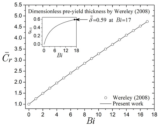
Figure 12. Dimensionless damping capacity ${\overline{C}}_r$ for different values of the Bingham number $Bi$ from the present work and the research reported by Wereley [22].

Conversely, semi-active controllable damping arises by applying a magnetic field to the MR fluid, reducing liquid transfer between the compression and rebound chambers during piston movement. In this figure, increasing the Bingham number $Bi$ enhances the damping capacity ${\overline{C}}_r$; $Bi=4.17$ doubles the Newtonian viscous damping (${\overline{C}}_r=2$), and $Bi=17$ generates ${\overline{C}}_r=4.74$. Furthermore, the results in Figure 12 correspond to the dimensionless damper force $\overline{F}$, considering that ${\overline{C}}_r=\overline{F}={\overline{C}}_{eq}{\overline{V}}_p/\left({\overline{C}}_{off}{\overline{V}}_p\right)$, where ${\overline{C}}_{eq}{\overline{V}}_p$ and ${\overline{C}}_{off}{\overline{V}}_p$ represent the damper force with and without a magnetic field [22]. Therefore, the parameter ${\overline{C}}_r=\overline{F}$ reflects the damper force that the MR valve opposes to the piston movement, thereby regulating flow through the valve.

In Figure 12, the Bingham number provides a general representation of the damping capacity of the MR valve. However, to explore the effect of adding hard spherical particles to the carrier fluid, Figure 13 and Figure 14 evaluate ${\overline{C}}_r$ involving $M_n$, which is directly related to the Bingham number $Bi$ in Equation (27). Therefore, Figure 13 presents the dimensionless damping capacity ${\overline{C}}_r$ as a function of the Mason number $M_n$, considering different critical Mason numbers $M_n^{*}$. In this figure, the Mason number $M_n$ represents the competition between magnetic and hydrodynamic stresses, and the critical Mason number $M_n^{*}$ exhibits the effect of the particle volume fraction $\varphi$ on the viscosity $\overline{\eta }$ and the yield stress ${\overline{\tau }}_0$. For this evaluation, the reference range $0.008\le M_n\le 0.018$ is derived from $0.2\le \varphi \le 0.3$ with ${\eta }_c=0.5$ Pa s, ${\dot{\gamma }}_c=9000$ s⁻¹, and $M_s=1600$ kA m⁻¹. Moreover, $M_n^{*}=0.0527$, $0.0827$, and $0.1097$ result from $\varphi =0.2$, $0.25$, and $0.3$, respectively. The reduction in $M_n$ from $0.018$ to $0.008$ implies that the magnetic stress increases with respect to the hydrodynamic stress. As a result, the fluid resistance increases as the Mason number decreases, thereby increasing the damping capacity. When $M_n$ decreases from $0.018$ to $0.008$, ${\overline{C}}_r$ with $M_n^{*}=0.0527$ increases from $2.42$ to $4.04$, while ${\overline{C}}_r$ with $M_n^{*}=0.1097$ rises from $1.7$ to $2.53$. Following this trend, the damping capacity benefits from the increase in $\varphi$ (via the critical Mason number) since ${\overline{C}}_r$ with $M_n^{*}=0.0527$ and $0.1097$ increases by $162\%$ and $83\%$ compared to the Newtonian viscous damping (${\overline{C}}_r=1$). Therefore, this evaluation between the critical Mason number and the Mason number provides a general estimate of the performance of the MR valve, considering as a reference measure the competition between magnetic and viscous stresses.

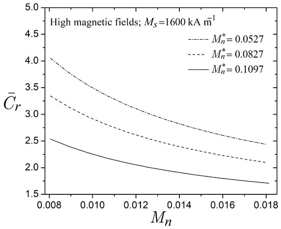
Figure 13. Dimensionless damping capacity ${\overline{C}}_r$ for different values of the critical Mason number $M_n^{*}$ and the Mason number $M_n$.

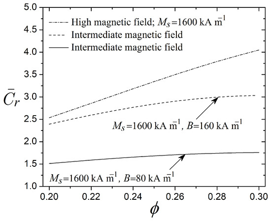
Figure 14. Dimensionless damping capacity ${\overline{C}}_r$ for different values of the particle volume fraction $\varphi$ and the magnetic field B.

On the other hand, Figure 14 shows the dimensionless damping capacity ${\overline{C}}_r$ as a function of the particle volume fraction $\varphi$, considering different magnetic fields. In this figure, Equation (28) establishes the fluid viscosity $\overline{\eta }$ in all cases, while Equations (7) and (8) determine the yield stress ${\overline{\tau }}_0$ for the intermediate and high magnetic fields. Furthermore, the damping capacity ${\overline{C}}_r$ is evaluated with fixed values of $M_n=0.008$ for the high magnetic field, as well as $M_n=0.0819$ and $0.3279$ for the intermediate magnetic fields of $B=160$ and 80 kA m⁻¹. The above Mason numbers assume as a reference $\varphi =0.2$, ${\eta }_c=0.5$ Pa s, ${\dot{\gamma }}_c=9000$ s⁻¹, and the corresponding magnetic fields. In the absence of magnetic particles $\varphi =0$, the damping of the MR valve recovers the Newtonian viscous damping of the carrier fluid. Conversely, when particles saturate at a high magnetic field, the damping capacity of the MR valve increases from ${\overline{C}}_r=2.53$ with $\varphi =0.2$ to ${\overline{C}}_r=4.04$ with $\varphi =0.3$, reflecting an increase in resistance to deformation. Meanwhile, the damping capacities at intermediate magnetic fields are ${\overline{C}}_r=2.39$ ($\varphi =0.2$) and $3.03$ ($\varphi =0.3$) when $B=160$ kA m⁻¹, and ${\overline{C}}_r=1.51$ ($\varphi =0.2$) and $1.75$ ($\varphi =0.3$) when $B=80$ kA m⁻¹. In the last case, when B increases from 80 to 160 kA m⁻¹, the damping capacity increases by $88\%$ when $\varphi =0.2$ and $128\%$ when $\varphi =0.3$ compared to Newtonian viscous damping (${\overline{C}}_r=1$). Also, the increase in the magnetic field magnifies the influence of the particle volume fraction $\varphi$. When $\varphi$ increases from $0.2$ to $0.3$, the damping capacity at the high magnetic field increases by $151\%$, while at intermediate magnetic fields, the damping capacity increases by $64\%$ when $B=160$ kA m⁻¹ and $24\%$ when $B=80$ kA m⁻¹. With these results, it is evident that magnetic particles in the carrier fluid play an essential role in the performance of the MR fluid, enhancing the damping capacity of the valve.

6. Conclusions

This work analyzes the hydrodynamic behavior of an MR valve, considering the microscopic characteristics of the fluid to form particle chain-like structures when a magnetic field is applied. Piston movement generates a pressure drop across the valve and induces liquid transfer between the compression and rebound chambers. Consequently, the physical properties of the MR fluid, such as viscosity, magnetic permeability, yield stress, and saturation magnetization, modify the flow rate by varying the resistance to deformation. The results reveal that valve control significantly depends on magnetic particles dispersed in the carrier fluid. The increase in particle volume fraction (via the Mason number) increases fluid resistance, thereby enhancing the damping capacity to regulate flow in the valve. Furthermore, the magnetic field influences the fluid performance since the magnetization of particles plays a vital role in the opening and closing of the valve. Therefore, from an application perspective, the proposed model in this research contributes to the understanding of the semi-active damping mechanism of MR valves by considering the microscopic characteristic of the fluid during the formation of particle chain-like structures that inhibit fluid motion, which have not been studied yet. Unlike traditional macroscopic models, the theoretical results obtained in this research exhibit the influence of magnetic particles on the carrier fluid, the non-linear magnetization of the MR fluid, the yield stress dependent on magnetic permeability, and the Mason number in the damping capacity of the MR valve. Finally, this work serves as a precedent for analyzing other types of dampers by adapting the operating mode to squeeze or shear, which promises to be a useful analytical tool in the design of devices based on MR fluids.

References

- Choi, S.-B.; Han, Y.-M. Magnetorheological Fluid Technology: Applications in Vehicle Systems, 1st ed.; CRC Press: Boca Raton, FL, USA, 2013; pp. 1–16. [Google Scholar]
- Bigué, J.-P.L.; Landry-Blais, A.; Pin, A.; Pilon, R.; Plante, J.-S.; Chen, X.; Andrews, M. On the relation between the Mason number and the durability of MR fluids. Smart Mater. Struct. 2019, 28, 094003. [Google Scholar] [CrossRef]
- Gołdasz, J.; Sapiński, B. Insight into Magnetorheological Shock Absorbers, 1st ed.; Springer: Cham, Switzerland, 2015; pp. 1–23. [Google Scholar]
- Zhang, Y.; Li, D.; Cui, H.; Yang, J. A new modified model for the rheological properties of magnetorheological fluids based on different magnetic field. J. Magn. Magn. Mater. 2020, 500, 166377. [Google Scholar] [CrossRef]
- Warke, V.; Kumar, S.; Bongale, A.; Kamat, P.; Kotecha, K.; Selvachandran, G.; Abraham, A. Improving the useful life of tools using active vibration control through data-driven approaches: A systematic literature review. Eng. Appl. Artif. Intell. 2024, 128, 107367. [Google Scholar] [CrossRef]
- De Vicente, J.; Klingenberg, D.J.; Hidalgo-Alvarez, R. Magnetorheological fluids: A review. Soft Matter 2011, 7, 3701–3710. [Google Scholar] [CrossRef]
- Berli, C.L.A.; De Vicente, J. A structural viscosity model for magnetorheology. Appl. Phys. Lett. 2012, 101, 021903. [Google Scholar] [CrossRef]
- Bica, I.; Liu, Y.D.; Choi, H.J. Physical characteristics of magnetorheological suspensions and their applications. J. Ind. Eng. Chem. 2013, 19, 394–406. [Google Scholar] [CrossRef]
- Khajehsaeid, H.; Alaghehband, N.; Bavil, P.K. On the yield stress of magnetorheological fluids. Chem. Eng. Sci. 2022, 256, 117699. [Google Scholar] [CrossRef]
- Kumar, S.; Sehgal, R.; Wani, M.F.; Sharma, M.D. Stabilization and tribological properties of magnetorheological (MR) fluids: A review. J. Magn. Magn. Mater. 2021, 538, 168295. [Google Scholar] [CrossRef]
- Carlson, J.D.; Jolly, M.R. MR fluid, foam and elastomer devices. Mechatronics 2000, 10, 555–569. [Google Scholar] [CrossRef]
- Dassisti, M.; Brunetti, G. Introduction to Magnetorheological Fluids. In Encyclopedia of Smart Materials; Olabi, A.-G., Ed.; Elsevier: Oxford, UK, 2022; pp. 187–202. [Google Scholar]
- Zeinali, M.; Mazlan, S.A.; Imaduddin, F.; Abd Fatah, A.Y.; Mughni, M.J.; Hamdan, L.H.; Mohd Yazid, I.I. Magnetorheological Fluid Characterization and Applications. In Reference Module in Materials Science and Materials Engineering; Elsevier: Amsterdam, The Netherlands, 2016; pp. 1–12. [Google Scholar]
- Gołdasz, J.; Sapiński, B.; Kubík, M.; Macháček, O.; Bańkosz, W.; Sattel, T.; Tan, A.S. Review: A survey on configurations and performance of flow-mode MR valves. Appl. Sci. 2022, 12, 6260. [Google Scholar] [CrossRef]
- Eshgarf, H.; Nadooshan, A.A.; Raisi, A. An overview on properties and applications of magnetorheological fluids: Dampers, batteries, valves and brakes. J. Energy Storage 2022, 50, 104648. [Google Scholar] [CrossRef]
- Shiao, Y.; Gadde, P.; Kantipudi, M.B. Energy-saving actuation signal for magnetorheological valve train by leveraging hysteresis effect. Energy Convers. Manag. X 2022, 16, 100292. [Google Scholar] [CrossRef]
- Kumar, J.S.; Alex, D.G.; Sam, P.P. Synthesis of magnetorheological fluid compositions for valve mode operation. Mater. Today Proc. 2020, 22, 1870–1877. [Google Scholar] [CrossRef]
- Salloom, M.Y. Modeling Behavior of Magnetorheological Fluids. In Encyclopedia of Smart Materials; Olabi, A.-G., Ed.; Elsevier: Oxford, UK, 2022; pp. 224–236. [Google Scholar]
- Chopra, I.; Sirohi, J. Smart Structures Theory; Cambridge University Press: New York, NY, USA, 2013; pp. 685–738. [Google Scholar]
- Özsoy, K.; Usal, M.R. A mathematical model for the magnetorheological materials and magneto reheological devices. Eng. Sci. Technol. Int J. 2018, 21, 1143–1151. [Google Scholar] [CrossRef]
- Parlak, Z.; Engin, T. Time-dependent CFD and quasi-static analysis of magnetorheological fluid dampers with experimental validation. Int. J. Mech. Sci. 2012, 64, 22–31. [Google Scholar] [CrossRef]
- Wereley, N.M. Nondimensional Herschel–Bulkley analysis of magnetorheological and electrorheological dampers. J. Intell. Mater. Syst. Struct. 2008, 19, 257–268. [Google Scholar] [CrossRef]
- Hong, S.-R.; John, S.; Wereley, N.M.; Choi, Y.-T.; Choi, S.-B. A unifying perspective on the quasi-steady analysis of magnetorheological dampers. J. Intell. Mater. Syst. Struct. 2008, 19, 959–976. [Google Scholar] [CrossRef]
- Manjeet, K.; Sujatha, C. Magnetorheological valves based on Herschel–Bulkley fluid model: Modelling, magnetostatic analysis and geometric optimization. Smart Mater. Struct. 2019, 28, 115008. [Google Scholar] [CrossRef]
- Jin, Z.; Guo, B.; Gao, S.; Wu, C.; Luo, Z.; Luo, K.; Liu, H. Rotational magnetorheological finishing of the interior surface of a small 316L stainless steel tube. J. Mater. Res. Technol. 2025, 36, 777–788. [Google Scholar] [CrossRef]
- Han, Z.; Su, B.; Li, Y.; Wang, W.; Wang, W.; Huang, J.; Chen, G. Numerical simulation of debris-flow behavior based on the SPH method incorporating the Herschel-Bulkley-Papanastasiou rheology model. Eng. Geol. 2019, 255, 26–36. [Google Scholar] [CrossRef]
- Ghaffari, A.; Hashemabadi, S.H.; Ashtiani, M. A review on the simulation and modeling of magnetorheological fluids. J. Intell. Mater. Syst. Struct. 2014, 26, 881–904. [Google Scholar] [CrossRef]
- Sherman, S.G.; Becnel, A.C.; Wereley, N.M. Relating Mason number to Bingham number in magnetorheological fluids. J. Magn. Magn. Mater. 2015, 380, 98–104. [Google Scholar] [CrossRef]
- Han, K.; Feng, Y.T.; Owen, D.R.J. Three-dimensional modelling and simulation of magnetorheological fluids. Int. J. Numer. Meth. Engng. 2010, 84, 1273–1302. [Google Scholar] [CrossRef]
- Wang, N.; Liu, X.; Sun, S.; Królczyk, G.; Li, Z.; Li, W. Microscopic characteristics of magnetorheological fluids subjected to magnetic fields. J. Magn. Magn. Mater. 2020, 501, 166443. [Google Scholar] [CrossRef]
- Klingenberg, D.J.; Ulicny, J.C.; Golden, M.A. Mason numbers for magnetorheology. J. Rheol. 2007, 51, 883–893. [Google Scholar] [CrossRef]
- Bossis, G.; Lacis, S.; Meunier, A.; Volkova, O. Magnetorheological fluids. J. Magn. Magn. Mater. 2002, 252, 224–228. [Google Scholar] [CrossRef]
- Wu, J.; Pei, L.; Xuan, S.; Yan, Q.; Gong, X. Particle size dependent rheological property in magnetic fluid. J. Magn. Magn. Mater. 2016, 408, 18–25. [Google Scholar] [CrossRef]
- Becnel, A.C.; Sherman, S.; Hu, W.; Wereley, N.M. Nondimensional scaling of magnetorheological rotary shear mode devices using the Mason number. J. Magn. Magn. Mater. 2015, 380, 90–97. [Google Scholar] [CrossRef]
- Melle, S.; Calderón, O.G.; Rubio, M.A.; Fuller, G.G. Microstructure evolution in magnetorheological suspensions governed by Mason number. Phys. Rev. E 2003, 68, 041503. [Google Scholar] [CrossRef] [PubMed]
- Wen, M.; Du, Y.; Liu, R.; Li, Z.; Rao, L.; Xiao, H.; Ouyang, Y.; Niu, X. Characterization of magnetorheological fluids based on capillary magneto-rheometer. Front. Mater. 2022, 9, 1034127. [Google Scholar] [CrossRef]
- Ginder, J.M.; Davis, L.C.; Elie, L.D. Rheology of magnetorheological fluids: Models and measurements. Int. J. Mod. Phys. B 1996, 10, 3293–3303. [Google Scholar] [CrossRef]
- Simon, T.M.; Reitich, F.; Jolly, M.R.; Ito, K.; Banks, H.T. The effective magnetic properties of magnetorheological fluids. Math. Comput. Model. 2001, 33, 273–284. [Google Scholar] [CrossRef]
- Mewis, J.; Wagner, N.J. Colloidal Suspension Rheology, 1st ed.; Cambridge University Press: New York, NY, USA, 2012; pp. 36–79. [Google Scholar]
- Lee, D.; Taylor, D.P. Viscous damper development and future trends. Struct. Des. Tall Build. 2001, 10, 311–320. [Google Scholar] [CrossRef]
- Vereda, F.; de Vicente, J.; Segovia-Gutíerrez, J.P.; Hidalgo-Alvarez, R. Average particle magnetization as an experimental scaling parameter for the yield stress of dilute magnetorheological fluids. J. Phys. D Appl. Phys. 2011, 44, 425002. [Google Scholar] [CrossRef]
- Goldasz, J.; Sapinski, B. Nondimensional characterization of flow-mode magnetorheological/electrorheological fluid dampers. J. Intell. Mater. Syst. Struct. 2012, 23, 1545–1562. [Google Scholar] [CrossRef]
Disclaimer/Publisher’s Note: The statements, opinions and data contained in all publications are solely those of the individual author(s) and contributor(s) and not of MDPI and/or the editor(s). MDPI and/or the editor(s) disclaim responsibility for any injury to people or property resulting from any ideas, methods, instructions or products referred to in the content. |
© 2025 by the authors. Licensee MDPI, Basel, Switzerland. This article is an open access article distributed under the terms and conditions of the Creative Commons Attribution (CC BY) license (https://creativecommons.org/licenses/by/4.0/).