Abstract
Collaborative clustering is an ensemble technique that enhances clustering performance by simultaneously and synergistically processing multiple data dimensions or tasks. This is an active research area in artificial intelligence, machine learning, and data mining. A common approach to co-clustering is based on non-negative matrix factorization (NMF). While widely used, NMF-based co-clustering is limited by its bilinear nature and fails to capture the multilinear structure of data. With the objective of enhancing the effectiveness of non-negative Tucker decomposition (NTD) in image clustering tasks, in this paper, we propose a dual-graph constrained sparse non-negative Tucker decomposition NTD (GDSNTD) model for co-clustering. It integrates graph regularization, the Frobenius norm, and an norm constraint to simultaneously optimize the objective function. The GDSNTD mode, featuring graph regularization on both factor matrices, more effectively discovers meaningful latent structures in high-order data. The addition of the regularization constraint on the factor matrices may help identify the most critical original features, and the use of the Frobenius norm may produce a more highly stable and accurate solution to the optimization problem. Then, the convergence of the proposed method is proven, and the detailed derivation is provided. Finally, experimental results on public datasets demonstrate that the proposed model outperforms state-of-the-art methods in image clustering, achieving superior scores in accuracy and Normalized Mutual Information.
MSC:
15A69; 62H30; 68U10
1. Introduction
Non-negative decomposition is a general term for a type of matrix or tensor decomposition method that requires all components in the decomposition result to be non-negative. The core idea is to decompose a non-negative data matrix or tensor into the product of several non-negative factor matrices or core tensors in order to extract interpretable latent features or components from non-negative data. The most representative non-negative decompositions are non-negative matrix factorization (NMF) and its extension in the high-dimensional domain non-negative Tucker decomposition (NTD). NMF is a common dimensionality reduction method that can extract the main features from the original data and has high interpretability [1]. When data requires more than two indices to be uniquely identified, it should be expressed in the form of a tensor. Thus, a tensor is naturally viewed as a generalization of vectors (first-order tensors) and matrices (second-order tensors) to higher orders. Non-negative tensor decomposition is a multi-dimensional data analysis method based on matrix decomposition, which can transform high-dimensional data into low-dimensional representations and retain the main features of the original data [2]. Shcherbakova et al. investigated the advantages of non-negative Tucker decomposition [3]. Like matrix decomposition, the purpose of tensor decomposition is to extract the information or main components hidden in the original data [4,5]. The Tucker decomposition is a tensor factorization method designed for handling tensor data [6]. NTD is a concrete application of Tucker decomposition in non-negative matrix decomposition. Its core idea is to decompose a high-order non-negative tensor into the product of a core tensor and a series of factor matrices [7]. NTD not only retains the interpretability benefits of NMF but also effectively preserves the inherent multi-way structure of the original tensor data. Consequently, non-negative Tucker decomposition (NTD) is extensively utilized in a wide range of disciplines, including image analysis and text mining, to uncover the latent structures inherent in multi-way datasets.
To improve model performance, numerous regularized extensions of NMF and NTD have been developed in the recent literature. These models have demonstrated excellent performance in image clustering or data mining. Cai et al. introduced the graph-regularized non-negative matrix factorization (GNMF) algorithm, which incorporates a geometrically-based affinity graph into the NMF framework to preserve the local manifold structure of the data [8]. Sun et al. proposed graph-regularized and sparse non-negative matrix factorization with hard constraints (GSNMFC), jointly incorporating a graph regularizer and hard prior label information as well as a sparseness constraint as additional conditions to uncover the intrinsic geometrical and discriminative structures of the data space [9]. They also proposed sparse dual graph-regularized non-negative matrix factorization (SDGNMF), jointly incorporating the dual graph-regularized and sparseness constraints as additional conditions to uncover the intrinsic geometrical, discriminative structures of the data space [10]. Shang et al. proposed a novel algorithm, called graph dual regularization non-negative matrix factorization (DNMF), which simultaneously considers the geometric structures of both the data manifold and the feature manifold [11]. Long et al. proposed a novel constrained non-negative matrix factorization algorithm, called the graph-regularized discriminative non-negative matrix factorization (GDNMF), to incorporate into the NMF model both the intrinsic geometrical structure and discriminative information [12]. Saberi-Movahed et al. present a systematic analysis of NMF in dimensionality reduction, with a focus on both feature extraction and feature selection approaches [13]. Jing et al. proposed a novel semi-supervised NMF method that incorporates label regularization, basis regularization, and graph regularization [14]. Li et al. developed a manifold regularization non-negative Tucker decomposition (MR-NTD) model. To preserve the geometric information within tensor data, their method employs a manifold regularization term on the core tensor derived from the Tucker decomposition [15]. Yin and Ma incorporated this geometrically based Locally Linear Embedding (LLE) into the original NTD, thus proposing NTD-LLE for the clustering of image databases [16]. To enhance the representation learning of tensor data, Qiu et al. proposed a novel graph-regularized non-negative Tucker decomposition (GNTD) framework [17]. This method is designed to jointly extract low-dimensional parts-based representations and preserve the underlying manifold structure within the high-dimensional tensor data.
The above research demonstrates that the non-negative decomposition model significantly improves image clustering performance. However, advancements in scientific technologies have led to increasingly complex phenomena, rendering previous models inadequate for handling the resulting complexities. Building on this foundation, a common strategy to enhance image clustering accuracy has been the development of collaborative clustering (co-clustering) frameworks. This is typically achieved by incorporating specific regularization terms that capture the relationships between different data views or clusters. Co-clustering is an ensemble learning method that performs simultaneous clustering along multiple dimensions or data views [18]. When using the non-negative matrix model, the goal of co-clustering is to simultaneously identify the clusters of both the rows and columns of the two-dimensional data matrix [19]. Del Buono and Pio present a process which aims at enhancing the performance of three-factor NMF as a co-clustering method, by identifying a clearer correlation structure represented by the block matrix [20]. Deng et al. proposed graph-regularized sparse NMF (GSNMF) and graph-regularized sparse non-negative matrix tri-factorization (GSNMTF) models. By incorporating an norm constraint on the low-dimensional matrix, they aimed to scale the data eigenvalues and enforce sparsity. This co-clustering approach has been shown to enhance the performance of standard non-negative matrix factorization models [21]. Chachlakis, Dhanaraj, Prater-Bennette, and Markopoulos presented Dynamic -Tucker: an algorithm for dynamic and outlier-resistant Tucker analysis of tensor data [22]. The norm is extensively used in convex optimization problems [23]. Ahmed et al. study a tensor-structured linear regression model over the space of sparse, low Tucker-rank tensors [24]. As deep learning models become larger and more complex, sparsity is emerging as a critical consideration for enhancing efficiency and scalability, making it a central theme in the development of new image processing and data analysis methods.
As illustrated by the above studies, building upon NMF, scholars have developed numerous models to address the evolving needs of various scientific fields. The performance of the NMF model can be significantly improved through the combined constraints of graph regularization and sparsity, which directly exploit the internal structure and inherent characteristics of the data. NTD is the extension of NMF to the high-dimensional domain. However, there are relatively few co-clustering methods for constructing high-performance NTD models that leverage the internal structure and inherent characteristics of the tensor data itself. While GNTD captures graph structure and sparse NMTF promotes sparsity, neither is designed to simultaneously learn from multiple graphs while enforcing directional sparsity patterns across different data modes. To address this gap, and inspired by advancements in co-clustering NMF, this paper proposes a GDSNTD model based on GNTD for enhanced co-clustering. The new model combines graph regularization, the Frobenius norm, and the norm to simultaneously optimize the objective function. In NTD, graph regularization serves to preserve the multi-linear structure of the original data. The review of the prior literature revealed that imposing multiple graph constraints on NMF models enhances their clustering performance. Motivated by this finding, we consequently introduce dual graph constraints into the NTD framework, applying them directly to the factor matrices of a tensor. This approach allows the model to capture the intrinsic data geometry more clearly, thereby improving clustering accuracy. Furthermore, we provide updated iterative optimization rules and prove the convergence of the model. Experiments on public datasets demonstrate that the proposed method outperforms several leading state-of-the-art methods.
The main contributions of this study are as follows:
- We introduce dual graph constraints into the NTD framework, applying them directly to the factor matrices of a tensor. To the best of our knowledge, no existing NTD framework integrates dual graph constraints with sparse regularization simultaneously. While graph-regularized and sparse factorization techniques exist, our model GDSNTD is the first to integrate them in a unified, constrained co-clustering optimization framework for NTD. We propose a new co-clustering version of the NTD model, equipped with three regularization terms: graph regularization, the Frobenius norm, and the norm. The graph regularization term captures the internal geometric structure of high-dimensional data more accurately. The norm term helps to scale original features in the factor matrices. The Frobenius norm improves the generalization ability of the model. Therefore, the co-clustering GDSNTD integrates strengths from graph-regularized and sparse factorization techniques so that the model yields a more accurate solution to the optimization problem.
- In the novel, unified optimization objective, we leverage the L-Lipschitz condition to derive the update rules for the proposed co-clustering GDSNTD method. Subsequently, we establish the convergence of the proposed algorithm.
- Experiments on public datasets demonstrate the effectiveness and superiority of the proposed method.
The remainder of the paper is organized as follows. In Section 2, we review the related models. In Section 3, the GDSNTD method is proposed, and its detailed inference process and the proof of convergence of the algorithm are illustrated. Section 4 presents the performance of the proposed model via experiments on various datasets. Finally, we present our conclusions in Section 5 and outline future work in Section 6.
2. Preliminaries
In this section, we review the related models.
- (A)
- NTDGiven a non-negative data tensor , non-negative tucker decomposition (NTD) aims at decomposing the non-negative tensor into a non-negative core tensor multiplied by N non-negative factor matrices , , and along each mode [7]. NTD minimizes the sum of squared residues between the data tensor and the multi-linear product of core tensor and factor matrices , , and , which is expressed asNTD provides an effective embedding and representation for image tensor data . However, NTD does not consider the geometrical structure of image tensor data .
- (B)
- GNTDQiu et al. [17] proposed the GNTD model, which incorporates the graph regularization term into the original NTD method. The GNTD is mathematically formulated aswhere is the regularization parameter for balancing the importance of the graph regularization term and the reconstruction error term, tr(·) denotes the trace of the matrix, and is a Laplacian matrix which characterizes the data manifold. is defined as , and . is the adjacency matrix of a p-nearest neighbor graph regarding the data points constructed using the scheme.where represents the set of p-nearest neighbor points of .The GNTD algorithm ingeniously combines graph constraints with non-negative constraints. This approach effectively preserves the local geometric structure of the data, enabling the learned features to better capture its intrinsic structure. As a result, GNTD significantly enhances the performance of traditional tensor decomposition models and has become a powerful tool for handling complex high-dimensional data, receiving considerable attention in machine learning and data mining.
- (C)
- GSNMTFThe graph-regularized sparse non-negative matrix tri-factorization (GSNMTF) model incorporates graph regularization and the norm into the standard NMF objective function [21]. This integration not only preserves the geometric structure of the data and feature spaces but also promotes sparsity in the resulting factor matrices. The objective function of GSNMTF is defined aswhere tr(·) is the trace of the matrix, and and are the parameters for controlling the sparseness of the matrices and , respectively. and are the Frobenius norm and norm, respectively.
3. Dual Graph Constraints into Sparse Non-Negative Tucker Decomposition (GDSNTD) Model
This section introduces the proposed GDSNTD model. We begin with the problem setup. Given a third-order tensor , where , , and are the numbers of rows, columns, and tubes of tensor, respectively. The Tucker decomposition of the tensor is given by
It decomposes a tensor into a core tensor multiplied by a matrix along each mode. Here the tensor is called the core tensor and its entries show the level of interaction between the different components. , , and are the factor matrices (which are usually orthogonal) and can be thought of as the principal components in each mode, and .
3.1. Data and Feature Graphs
Many research studies have demonstrated that geometric structure not only affects the data space but also the feature space and that high-dimensional data are usually located in a low-dimensional sub-manifold of the ambient space, and this underlying geometrical information of data could be obtained by modeling a neighbor graph. We impose a graph regularization constraint on the factor matrix . We construct a p-nearest neighbors data space, whose vertices are . Then, we encode their geometrical information by connecting each tensor subject with its p-nearest neighbors, thereby constructing a p-nearest neighbor graph [8] with a binary weighting scheme. The weight matrix is defined as
where represents the set of p samples closest to in the graph. The graph Laplacian of the data graph is defined as , where is the diagonal degree matrix whose elements are given by .
Similarly, we impose a graph regularization constraint on the factor matrix . We can also construct a p-nearest neighbors graph of the feature space and define the weight matrix as follows:
where represents the set of p samples closest to in the graph. The graph Laplacian of the data graph is defined as .
3.2. Objective Function of GDSNTD
In this part, we present our objective function of GDSNTD, which is designed to approximate the original high-dimensional tensor by yielding cleaner and sparser low-dimensional matrices. This model is able to present the geometric structure of tensors more clearly than GNTD and makes up for the deficiency of GSNMTF in handling high-dimensional data. The proposed model has advanced the development of the NTD framework by improving its convergence properties and has facilitated its application in complex tasks such as image clustering analysis. It integrates graph regularization, the Frobenius norm, and a sparsity constraint, and its objective function is defined as
where tr(·) is the trace of the matrix. is the parameter of , is the parameter of . and are the graph regularization parameters of and , respectively. They govern the trade-off between preserving the intrinsic graph structure of the data and optimizing other objective terms. and are coefficients of the norm. They serve as a trade-off between the sparsity of the factor matrices and other objective terms. It is worth noting that the norms in the objective function are entrywise norms [25]. and represent the Frobenius norm and norm, respectively.
Equivalently, Equation (2) is to be rewritten in matrix form as
where the tensor is expanded according to mode-1. When the tensor is expanded according to mode-2 or mode-3, it is to be rewritten in the following forms as Equations (4) and Equation (5), respectively:
3.3. Inference of GDSNTD
In this section, the detailed inference is illustrated, and then, a corresponding algorithm is designed.
3.3.1. Fix , , , Solve
Letting be the Lagrange multiplier [26] for constraint , and our objective function is written in matrix form as
To obtain the optimal solution, the gradient descent algorithm [27] is used to solve Equation (6). The gradient is as follows:
Let represent the corresponding value during the tth round of updates. Therefore, using the Karush–Kuhn–Tucker (KKT) condition [27], and , we obtain the following updating rule:
3.3.2. Fix , and , Solve
At this stage, similar to the update of , letting be the Lagrange multiplier for constraint , our optimization goal is to be written in matrix form as follows:
The function (10) is to be rewritten as
Now, the partial derivative of to is
According to the (Karush–Kuhn–Tucker) (KKT) condition [27], , so
And also because , ⊙ denotes the Hadamard product, and we can obtain the following:
Therefore, the update rule of is
3.3.3. Fix , and , Solve
At this stage, our goal is to minimize the function . The optimization goal in (4) is to be defined as
where
Since is a convex function with respect to and it satisfies the L-Lipschitz condition [28] as shown in Equation (14), there exists a constant such that
where is to be by the approximated second-order Taylor expansion near as
Let , the minimum value of Equation (17) is then obtained as and
Since is independent of the optimization variable , it can be treated as a constant. Consequently, the objective function for updating simplifies to
Let , then, for solving Equation (19), we first solve and then
Now, the partial derivative of to is
where and should be solved at the same time. According to the (Karush–Kuhn–Tucker) (KKT) condition [27], , and , we can obtain the following:
Therefore, the update rule of is
To solve the objective function in Equation (19), we minimize the term using the gradient descent and apply a soft threshold [28] to minimize the regularizer. Consequently, the update rule for is derived as follows:
3.3.4. Fix , and , Solve
Similarly, to update the factor matrix , we write the objective function as follows:
where
Since in Equation (25) is a convex function regarding , and satisfies the L-Lipschitz condition [28], there exists a constant such that
where is the derivative of . is to be by the approximated second-order Taylor expansion near as
Let , then, the minimum value of Equation (28) is obtained as and
Similarly, since is independent of , the objective function updated with can be written as
Let , then, for solving Equation (30), we first solve and then
Now, the partial derivative of to is
where and should be solved at the same time. According to the (Karush–Kuhn–Tucker) (KKT) condition [27], , and , we can obtain the following:
Therefore, the update rule of is
Similarly, we minimize and using gradient descent and soft thresholding, respectively. This leads to the following update rule for :
3.4. Algorithm Design
According to the above reasoning, a clustering algorithm based on GDSNTD is summarized, with its detailed steps outlined in Algorithm 1.
| Algorithm 1: GDSNTD for Clustering |
|
We employ a stopping criterion based on the relative change in the objective function value. The criterion is defined as
where and are the objective function values at the -th and k-th iterations, respectively. The iterations are terminated when , with being a predefined convergence tolerance [29].
3.5. Convergence Analysis
Since the update rule for is identical to that in [17], this subsection employs the auxiliary function approach exclusively to prove the convergence of the updating rules given in Equations (8), (13), (24) and (35). We now present the following theorem:
Theorem 1.
To prove Theorem 1, we first give a definition and several lemmas.
Definition 1
([1]). is an auxiliary function for if the conditions and are satisfied.
Lemma 1
([1]). If is an auxiliary function for , then is non-increasing under the updating rule
Proof.
. □
The equality holds only if is a local minimum of . By iterating the update rule (36), converges to the local minimum of .
Next, we provide a detailed proof of the convergence for the above updating rule for using an auxiliary function. Recall the function from Equation (3):
We can obtain
Essentially, it is sufficient to prove that each is non-increasing under the update rule.
Lemma 2.
The function
is an auxiliary function for , where the matrix .
Proof.
Obviously, . According to Definition 1, we only need to show that ≥. We first obtain the Taylor series expansion of at to be
By Equation (40), ≥ is equivalent to
We can obtain
Therefore, the inequality ≥ holds. □
Analogously, the convergence under the update rule in Equation (24) can be proven. Next, we provide a detailed proof of convergence for the update rule using an auxiliary function. Consider the following function:
where
We derive
Essentially, the updating rule is element wise, so it is sufficient to prove each is non-increasing under the update rule.
Lemma 3.
The function
is an auxiliary function for , where the matrix , and
Proof.
The soft thresholding operation ensures convergence as follows: if , the update subtracts a constant value; otherwise, if , the value is set to zero. Both cases are consistent with the convergence proof. Because Equation (51) is an auxiliary function for , and according to the soft threshold, is non-increasing under the updating rule stated in Equation (24). Analogously, we can prove the convergence under the updating rule in Equation (35).
4. Experiments
In this section, the experimental setup and analysis of the results are discussed in detail. The descriptions of these datasets are given as follows. First, we introduce the image datasets Coil20 (http://www.cad.zju.edu.cn/home/dengcai/Data/MLData.html, (accessed on 15 May 2024)), Georgia (https://www.cnblogs.com/kuangqiu/p/7776829.html, (accessed on 10 March 2025)), Iris (http://archive.ics.uci.edu/dataset/53/iris, (accessed 20 November 2024)) [30]. The datasets are summarized in Table 1.

Table 1.
Summary of the datasets.
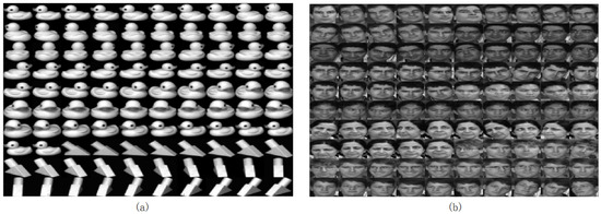
Figure 1.
The details of public datasets of Coil20 (a) and Georgia (b).
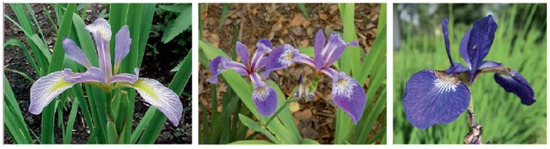
Figure 2.
Different kinds of Iris datasets.
In order to evaluate the effectiveness of our proposed GDSNTD scheme, we compared it with six classical or state-of-the-art clustering and co-clustering methods. All the simulations were performed on a computer with a 2.30-GHz Intel Core i7-11800H CPU and 32 GB memory of 64-bit MATLAB 2016a in Windows 10. Without special specifications, the maximum number of iterations is set to 1000.
- Non-negative matrix factorization (NMF) [1]: NMF aims to decompose a matrix into two low-dimensional matrices and is now often used as a data processing method in machine learning.
- Non-negative Tucker decomposition (NTD) [7]: The NTD algorithm is considered as a generalization of NMF.
- Graph-regularized NTD (GNTD) [17]:
- Graph dual regularized NMF (GDNMF) [12]: GDNMF simultaneously considers the geometric structures of both the data manifold and the feature manifold.
- Graph dual regularized non-negative matrix tri-factorization (GDNMTF) [12]: DNMTF is an extension of our DNMF algorithm and simultaneously incorporates two graph regularizers of both data manifold and feature manifold into its objective function.
- Graph-regularized sparse non-negative matrix trifactorization (GSNMTF) [21]: The GSNMTF model introduces graph regularization and an norm constraint into the objective function.
4.1. Evaluation Measures
In this section, two widely used metrics, accuracy (AC) and Normalized Mutual Information (NMI), are used to evaluate the clustering performance. Accuracy aims to find a one-to-one relationship between classes and clusters. It is usually used to calculate the proportion of correct samples to the total number of samples. It is a relatively intuitive evaluation index. Accuracy is a clustering evaluation metric that measures the proportion of correctly assigned samples against the total, after a one-to-one mapping between clusters and true classes is established. It is an intuitive and widely used measure [31]. NMI is commonly used in clustering to measure the similarity between two clusterings.
AC is defined as
where N is the total number of samples, is the ground-truth label of sample i, is the cluster label assigned by the algorithm, is the Dirac delta function, and is the optimal mapping function [32].
NMI is defined as
where is the mutual information between B and T, and and are their entropies. A higher NMI indicates a better alignment between the clustering result and the true labels [33].
4.2. Experimental Setup and Clustering Results Analysis
In this part, the experimental setup is described, and the experimental results are discussed in detail. To ensure the fairness between models, our proposed algorithm and all comparison algorithms use the same random initialization matrix. Subsequently, each experiment is conducted ten times independently on original data, then K-means clustering is performed five times independently on this low-dimensional reduced data. The average and variance of the results are recorded. The standard deviation is set to 0 if it is less than .
Table 2 and Table 3 summarize the accuracy and NMI results for each algorithm across all datasets. Table 4 lists the accuracy and standard deviation for each algorithm on the Georgia dataset, while Table 5 presents the corresponding NMI results. Similarly, results for the COIL20 dataset are detailed in Table 6 (accuracy) and Table 7 (NMI). From the results, we derive the following main conclusions:
Table 2.
AC (%) of each algorithm on each dataset.
Table 3.
NMI (%) of each algorithm on each dataset.
Table 4.
AC (%) of each algorithm on Georgia dataset.
Table 5.
NMI (%) of each algorithm on Georgia dataset.
Table 6.
AC (%) of each algorithm on Coil20 dataset.
Table 7.
NMI (%) of each algorithm on Coil20 dataset.
- 1.
- From Table 2, we can observe that the value of AC of GDSNTD is better than that of other methods on most datasets. The value of NMI reflects the proportion of correct decisions, which also proves that the proposed model performs better. The performance improvement is evident in the Georgia dataset, where GDSNTD improves the accuracy by 48.92% over the NMF co-clustering algorithm. The accuracy of GDSNTD is also improved by 26.1%, 5.15%, 7.02%, 3.71%, and 2.82% compared with other co-clustering algorithms NTD, GNTD, GDNMF, GDNMTF, and GSNMTF, respectively. In the Coil20 dataset, the accuracy of GDSNTD is also improved by 30.50%, 38.58%, 2.29%, 0.81%, 1.14%, and 0.57%, compared with other co-clustering algorithms NTD, GNTD, GDNMF, GDNMTF, and GSNMTF, respectively. In the Iris dataset, the accuracy of GDSNTD is improved by 17.22%, 32.77%, 2.84%, 2.10%, 0.17%, and 0.12% compared with other co-clustering algorithms NMF, NTD, GNTD, GDNMF, GDNMTF, and GSNMTF, respectively.
- 2.
- From Table 3, we can observe that our proposed method of GDSNTD can also achieve higher accuracy. The NMI of GDSNTD is as high as 50.16% on the Iris dataset, which is 34.95%, 7.46%, 4.27%, 3.49%, and 3.42% better compared with NMF, GNTD, GDNMF, GDNMTF, and GSNMTF, respectively. In the Georgia dataset, the accuracy of GDSNTD is also improved by 26.67%, 15.01%, 3.12%, 4.79%, 4.54%, and 4.26% compared with other co-clustering algorithms NMF, NTD, GNTD, GDNMF, GDNMTF, and GSNMTF, respectively. In the Coil20 dataset, the accuracy of GDSNTD is improved by 21.02%, 23.85%, 2.75%, 0.3%, 0.2%, and 0.32%, compared with other co-clustering algorithms NMF, NTD, GNTD, GDNMF, GDNMTF, and GSNMTF, respectively.
- 3.
- Table 4 shows that the average AC of GDSNTD is higher than that of the other methods on most datasets. In the Georgia dataset, the accuracy of the co-clustering algorithm GDSNTD is improved by an average of 27.4%, 22.6%, 2.2%, 8.7%, 5.11%, and 3.79% compared with NMF, NTD, GNTD, GDNMF, GDNMTF, and GSNMTF, respectively. From Table 6, it can be observed that on the Coil20 dataset, the accuracy of GDSNTD is, on average, 23.9%, 30.9%, 1.49%, 4.0%, 5.79%, and 3.18% higher than that of NMF, NTD, GNTD, GDNMF, GDNMTF, and GSNMTF, respectively.
- 4.
- From Table 5, it can be observed that on the Georgia dataset, the accuracy of GDSNTD is, on average, 23.7%, 19.4%, 1.82%, 7.3%, 5.67%, and 4.63% higher than that of NMF, NTD, GNTD, GDNMF, GDNMTF, and GSNMTF, respectively. From Table 7, it can be observed that on the Coil20 dataset, the accuracy of GDSNTD is, on average, 20.8%, 31.5%, 1.42%, 3.2%, 6.14%, and 2.76% higher than that of NMF, NTD, GNTD, GDNMF, GDNMTF, and GSNMTF, respectively.
Figure 3 shows the clustering performance on the Georgia, COIL20, and Iris datasets. It can be observed that the proposed GDSNTD method surpasses all other compared methods.
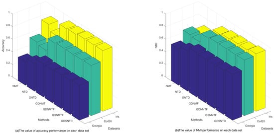
Figure 3.
The clustering performance on each dataset.
4.3. Interpretation of GDSNTD’s Superior Performance
Across all datasets, our proposed method consistently outperforms all competing baselines of NMF, NTD, GNTD, GDNMF, GDNMTF, and GSNMTF in both standard clustering and co-clustering tasks. This empirical evidence strongly suggests that the GDSNTD model with dual graph constraints successfully leads to a more structured and discriminative latent space, thereby improving clustering accuracy.
First, applying manifold constraints to the factor matrices is equivalent to preserving the structure in the “essential features” of the data, resulting in greater accuracy. Second, regularization counterbalances the Frobenius norm, leading to a more stable optimization process and yielding factors within a more reasonable numerical range. Furthermore, regularization promotes the learning of “parts” that correspond to local structures within the data, thereby promoting a decomposition with enhanced coherence.
4.4. Parameter Selection
Every parameter is searched over a range of values from 0 to . The choice of parameters has a pronounced effect on experimental performance; therefore, they were selected systematically through a grid search. Figure 4 shows the process of determining the optimal parameters using a grid search on the Iris dataset. From Figure 4, we can see that the accuracy is only when and . When the coefficient of the sparse regularization term is , the accuracy improves to . From Figure 5, it is to be observed that the NMI is when and , and when the coefficient of the sparse regularization term is , the accuracy is only .
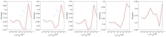
Figure 4.
Parameter tuning on dataset Coil20 regarding accuracy.
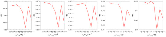
Figure 5.
Parameter tuning on dataset Coil20 regarding NMI.
4.5. Convergence Study
As described in Section 3, the convergence of the proposed algorithms has been theoretically proved. In this subsection, we experimentally analyze the convergence of the proposed algorithms by examining the relationship between the number of iterations and the value of the objective function. This relationship is visualized in Figure 6, Figure 7 and Figure 8. The convergence behavior of GSNTD on the Georgia dataset is illustrated in Figure 6. The convergence behavior of GSNTD on the Coil20 dataset is illustrated in Figure 7. The convergence behavior of GSNTD on the Iris dataset is illustrated in Figure 8. The observed monotonic decrease in the objective function value demonstrates that the algorithm converges effectively under the multiplicative update rules. This result provides empirical support for the convergence proof given in Theorem 1. We can find that GDSNTD is usually able to reach convergence within 1000 iterations.
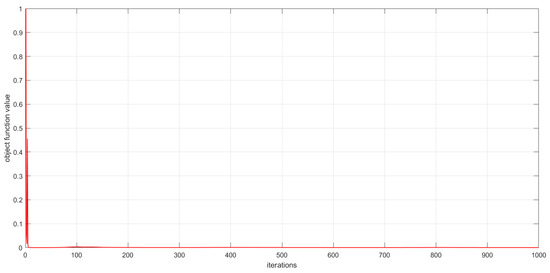
Figure 6.
Convergence curves of GDSNTD on Georgia dataset.
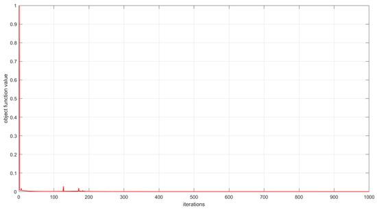
Figure 7.
Convergence curves of GDSNTD on Coil20 dataset.
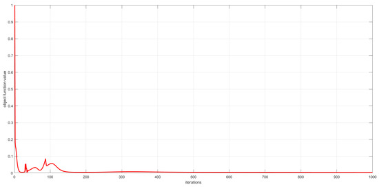
Figure 8.
Convergence curves of GDSNTD on Iris dataset.
4.6. Complexity Analysis
In this subsection, we analyze the computational complexity of GDSNTD. Note that is a third-order -dimensional tensor, and is a third-order -dimensional core tensor. Factor matrices are , , and .
Consider the updating rule in (8), the operation corresponds to the tensor mode product . Its computational complexity is . corresponds to . The computational complexity is . The total computational complexity of computing the update of is bounded by .
Consider the updating rule in (13), corresponds to , which needs operations. corresponds to , which needs operations. The total computational complexity of computing the update of is bounded by .
Consider the updating rule in (23), corresponds to , and it takes operations. corresponds to , and it takes operations. The total computational complexity of computing the update of is bounded by .
Similarly, consider the updating rule in (34), the total computational complexity of computing the update of is bounded by .
Therefore, the total computational complexity of the proposed method is . Compared with GNTD, the total computational complexity of the GDSNTD is increased by .
Figure 9 shows the relative performance in terms of clustering ACC and time consumption among NTD, GNTD, GDNMTF, GSNMTF, and GDSNTD on the Georgia dataset. Figure 10 shows the relative performance in terms of clustering NMI and time consumption among NTD, GNTD, GDNMTF, GSNMTF, and GDSNTD on the Coil20 dataset. In the figure, CPU(s) is the running time in seconds.
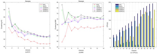
Figure 9.
Comparison of clustering performance and running time among NTD, GNTD, GDNMTF, GSNMTF, and GDSNTD on the Coil20 dataset.
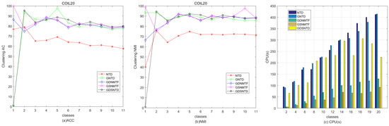
Figure 10.
Comparison of clustering performance and running time among NTD, GNTD, GDNMTF, GSNMTF, and GDSNTD on the Georgia dataset.
5. Conclusions
In this paper, we propose a co-clustering method via a dual graph-regularized sparse non-negative Tucker decomposition (GDSNTD) framework. It incorporates the Frobenius norm, graph regularization, and an norm constraint. The graph regularization term is used to maintain the intrinsic geometric structure of the data. This approach allows the model to represent the internal structure of high-dimensional data more accurately. The model not only adds the norm to achieve the adjustment of data eigenvalues but also embeds the Frobenius norm to improve the generalization ability of the model. We then present a detailed derivation of the solution, design the accompanying algorithm for GDSNTD, and provide a convergence proof. The experimental results show that selecting appropriate parameters can improve the model’s classification accuracy. This indicates that the selected rules have practical significance. Experiments on public datasets demonstrate that our proposed model achieves superior image clustering performance. The proposed method outperforms the state-of-the-art method GSNMTF by an average of 3.79% in clustering accuracy and 4.63% in Normalized Mutual Information on the Georgia dataset.
6. Future Work
Although the proposed GSNTTD method has shown good clustering performance, it operates on the assumption that the data resides in a well-formed latent vector space [34]. In recent years, deep learning-based clustering has experienced rapid advancement. The current popular deep learning-based methods are dominated by several key approaches, such as Graph Autoencoders (GAEs), graph convolutional network-based clustering (GCN-based clustering), and Deep Tensor Factorization.
GAEs aim to learn low-dimensional latent representations (embeddings) of graph-structured data in an unsupervised manner. It learns to compress input data into a lower-dimensional latent representation (encoding) and then reconstruct the original input from this representation (decoding). The critical distinction is that the input data is a graph, characterized by its topology (structure) and node attributes (features). Kipf et al. in [35] formally introduced the GAE and its variational counterpart, the variational graph autoencoder (VGAE). The field of GAE has evolved rapidly from foundational models to highly sophisticated and specialized architectures. Recent advancements have focused on developing more sophisticated architectures to address specific challenges. Zhou K et al. proposed a new causal representation method based on a graph autoencoder embedded autoencoder (GeAE). The GeAE employs a causal structure learning module to account for non-linear causal relationships present in the data [36].
Kipf and Welling in [35] introduced the variational graph autoencoder (VGAE), a framework for unsupervised learning on graph-structured data based on the variational autoencoder (VAE). In this work, they demonstrated this VGAE model using a GCN encoder and a simple inner product decoder. In [37], Kipf and Welling first introduced the efficient, first-order approximation-based graph convolutional layer. This formulation has laid the groundwork for numerous subsequent GCN studies. The core idea of a GCN encoder is to learn low-dimensional vector representations (i.e., node embeddings) for nodes by propagating and transforming information across the graph structure. The node’s embedding is determined not only by its own features but also jointly by the features of its neighbor nodes and the local graph structure. The core principle of GCN-based clustering is to unify node representation learning and cluster assignment into an end-to-end, jointly optimized framework and perform these tasks simultaneously.
The principle of Deep Tensor Factorization can be understood as using a deep neural network to perform the factorization and reconstruction process. Wu et al. proposed a Neural Tensor Factorization model, which incorporates a multi-layer perceptron structure to learn the non-linearities between different latent factors [38]. In [39], Jiang et al. proposed a generic architecture of deep transfer tensor factorization (DTTF), where the side information is embedded to provide effective compensation for the tensor sparsity.
In [40], Ballard et al. categorized feedforward neural networks, graph convolutional neural networks, and autoencoders into non-generative deep learning-based multi-omics integration methods. They found that deep learning-based approaches build off of previous statistical methods to integrate multi-omics data by enabling the modeling of complex and non-linear interactions between data types. Therefore, deep learning-based clustering has emerged as a rapidly advancing field. It integrates conventional cluster analysis with deep learning, leveraging its powerful feature representation and non-linear mapping capabilities to demonstrate superior performance in unsupervised clustering tasks. In the future, we intend to incorporate recent deep learning-based methods into our subsequent research to explore more up-to-date clustering methodologies.
Author Contributions
Conceptualization, J.H. and L.L.; methodology, L.L.; writing—original draft preparation J.H. and L.L. All authors have read and agreed to the published version of the manuscript.
Funding
The authors acknowledge the support from the National Natural Science Foundation of China under Grants (Nos. 12361044, 12161020, 12061025), Basic Research Project of Science and Technology Plan of Guizhou of China under Grants Qian Ke he foundation ZK[2023] General 022.
Data Availability Statement
The original contributions presented in this study are included in the article, further inquiries can be directed to the corresponding author.
Conflicts of Interest
The authors declare no conflict of interest. The authors declare that they have no known competing financial interests or personal relationships that could have appeared to influence the work reported in this paper.
References
- Lee, D.; Seung, H.S. Learning the parts of objects by non-negative matrix factorization. Nature 1999, 401, 788–791. [Google Scholar] [CrossRef] [PubMed]
- Friedlander, M.P.; Hatz, K. Computing non-negative tensor factorizations. Optim. Methods Softw. 2008, 23, 631–647. [Google Scholar] [CrossRef]
- Shcherbakova, E.M.; Matveev, S.A.; Smirnov, A.P.; Tyrtyshnikov, E.E. Study of performance of low-rank nonnegative tensor factorization methods. Russ. J. Numer. Anal. Math. Model. 2023, 38, 231–239. [Google Scholar] [CrossRef]
- De Lathauwer, L. A survey of tensor methods. In Proceedings of the 2009 IEEE International Symposium on Circuits and Systems, Taipei, Taiwan, 24–27 May 2009; pp. 2773–2776. [Google Scholar] [CrossRef]
- Zhou, G.; Cichocki, A.; Zhao, Q.; Xie, S. Nonnegative matrix and tensor factorizations: An algorithmic perspective. IEEE Signal Process. Mag. 2014, 31, 54–65. [Google Scholar] [CrossRef]
- Kolda, T.G.; Bader, B.W. Tensor decompositions and applications. SIAM Rev. 2009, 51, 455–500. [Google Scholar] [CrossRef]
- Kim, Y.D.; Choi, S. Nonnegative Tucker decomposition. In Proceedings of the 2007 IEEE Conference on Computer Vision and Pattern Recognition, Minneapolis, MN, USA, 17–22 June 2007; IEEE: New York, NY, USA, 2007; pp. 1–8. [Google Scholar] [CrossRef]
- Cai, D.; He, X.; Han, J.; Huang, T.S. Graph regularized nonnegative matrix factorization for data representation. IEEE Trans. Pattern Anal. Mach. Intell. 2010, 33, 1548–1560. [Google Scholar] [CrossRef]
- Sun, F.; Xu, M.; Hu, X.; Jiang, X. Graph regularized and sparse nonnegative matrix factorization with hard constraints for data representation. Neurocomputing 2016, 173, 233–244. [Google Scholar] [CrossRef]
- Sun, J.; Wang, Z.H.; Sun, F.; Li, H.J. Sparse dual graph-regularized NMF for image co-clustering. Neurocomputing 2018, 316, 156–165. [Google Scholar] [CrossRef]
- Shang, F.; Jiao, L.C.; Wang, J. Graph dual regularization non-negative matrix factorization for co-clustering. Pattern Recognit. 2012, 45, 2237–2250. [Google Scholar] [CrossRef]
- Long, X.; Lu, H.; Peng, Y.; Li, W. Graph regularized discriminative non-negative matrix factorization for face recognition. Multimed. Tools Appl. 2014, 72, 2679–2699. [Google Scholar] [CrossRef]
- Saberi-Movahed, F.; Berahm, K.; Sheikhpour, R.; Li, Y.; Pan, S. Nonnegative matrix factorization in dimensionality reduction: A survey. arXiv 2024, arXiv:2405.03615. [Google Scholar] [CrossRef]
- Jing, W.J.; Lu, L.; Ou, W. Semi-supervised non-negative matrix factorization with structure preserving for image clustering. Neural Netw. 2025, 187, 107340. [Google Scholar] [CrossRef]
- Li, X.; Ng, M.K.; Cong, G.; Ye, Y.; Wu, Q. MR-NTD: Manifold Regularization Nonnegative Tucker Decomposition for Tensor Data Dimension Reduction and Representation. IEEE Trans. Neural Netw. Learn. Syst. 2016, 28, 1787–1800. [Google Scholar] [CrossRef]
- Yin, W.; Ma, Z. LE & LLE Regularized Nonnegative Tucker Decomposition for clustering of high dimensional datasets. Neurocomputing 2019, 364, 77–94. [Google Scholar] [CrossRef]
- Qiu, Y.; Zhou, G.; Zhang, Y.; Xie, S. Graph regularized nonnegative Tucker decomposition for tensor data representation. In Proceedings of the ICASSP 2019—2019 IEEE International Conference on Acoustics, Speech and Signal Processing (ICASSP), Brighton, UK, 12–17 May 2019; IEEE: New York, NY, USA, 2019; pp. 8613–8617. [Google Scholar] [CrossRef]
- Dhillon, I.S.; Mallela, S.; Modha, D.S. Information-theoretic co-clustering. In Proceedings of the Ninth ACM SIGKDD International Conference on Knowledge Discovery and Data Mining, Washington, DC, USA, 24–27 August 2003; pp. 89–98. [Google Scholar] [CrossRef]
- Whang, J.J.; Dhillo, I.S. Non-exhaustive, Overlapping co-clustering. In Proceedings of the 2017 ACM on Conference on Information and Knowledge Management, Singapore, 6–10 November 2017; pp. 2367–2370. [Google Scholar] [CrossRef]
- Del Buono, N.; Pio, G. Non-negative matrix tri-factorization for co-clustering: An analysis of the block matrix. Inf. Sci. 2015, 301, 13–26. [Google Scholar] [CrossRef]
- Deng, P.; Li, T.R.; Wang, H.; Wang, D.; Horng, S.J.; Liu, R. Graph Regularized Sparse Non-Negative Matrix Factorization for Clustering. IEEE Trans. Comput. Soc. Syst. 2023, 10, 910–921. [Google Scholar] [CrossRef]
- Chachlakis, D.G.; Dhanaraj, M.; Prater-Bennette, A.; Markopoulos, P.P. Dynamic L1-norm Tucker tensor decomposition. IEEE J. Sel. Top. Signal Process. 2021, 15, 587–602. [Google Scholar] [CrossRef]
- Peng, X.; Lu, C.Y.; Yi, Z.; Tang, H.J. Connections Between Nuclear-Norm af Frobenius-Norm-Based Representations. IEEE Trans. Neural Netw. Learn. Syst. 2016, 29, 218–224. [Google Scholar] [CrossRef]
- Ahmed, T.; Raja, H.; Bajwa, W.U. Tensor regression using low-rank and sparse Tucker decompositions. SIAM J. Math. Data Sci. 2020, 2, 944–966. [Google Scholar] [CrossRef]
- Chachlakis, D.G.; Prater-Bennette, A.; Markopoulos, P.P. L1-norm Tucker tensor decomposition. IEEE Access 2019, 7, 178454–178465. [Google Scholar] [CrossRef]
- Rockafellar, R.T. Lagrange multipliers and optimality. SIAM Rev. 1993, 35, 183–238. [Google Scholar] [CrossRef]
- Stephen, B.; Lieven, V. Convex Optimization; Cambridge University Press: Cambridge, UK, 2004. [Google Scholar] [CrossRef]
- Patrick, L.C.; Valérie, R.W. Signal recovery by proximal forward-backward splitting. Multiscale Model. Simul. 2005, 4, 1168–1200. [Google Scholar] [CrossRef]
- Kim, H.; Park, H. Nonnegative matrix factorization based on alternating nonnegativity constrained least squares and active set method. SIAM J. Matrix Anal. Appl. 2008, 30, 713–730. [Google Scholar] [CrossRef]
- Asuncion, A.; Newman, D. Iris; UCI Machine Learning Repository: Irvine, CA, USA, 1936. [Google Scholar] [CrossRef]
- Cai, D.; He, X.; Han, J. Document clustering using locality preserving indexing. IEEE Trans. Knowl. Data Eng. 2005, 17, 1624–1637. [Google Scholar] [CrossRef]
- Yang, C.; Yi, Z. Document clustering using locality preserving indexing and support vector machines. Soft Comput. 2008, 17, 677–683. [Google Scholar] [CrossRef]
- Estévez, P.A.; Tesmer, M.; Perez, C.A.; Zurada, J.M. Normalized mutual information feature selection. IEEE Trans. Neural Netw. 2009, 20, 189–201. [Google Scholar] [CrossRef]
- Dong, Y.; Deng, Y.; Dong, Y.; Wang, J. A survey of clustering based on deep learning. Comput. Appl. 2022, 42, 1021–1028. [Google Scholar] [CrossRef]
- Kipf, T.N.; Welling, M. Variational Graph Auto-Encoders. Neural Information Processing Systems (NeurIPS) Workshop on Bayesian Deep Learning. arXiv 2016, arXiv:1611.07308. [Google Scholar] [CrossRef]
- Zhou, K.; Jiang, M.; Gabrys, B.; Xu, Y. Learning causal representations based on a GAE embedded autoencoder. IEEE Trans. Knowl. Data Eng. 2025, 37, 3472–3484. [Google Scholar] [CrossRef]
- Kipf, T.N.; Welling, M. Semi-supervised classification with graph convolutional networks. arXiv 2016, arXiv:1609.02907v4. [Google Scholar] [CrossRef]
- Wu, X.; Shi, B.; Dong, Y.; Huang, C.; Chawla, N.V. Neural tensor factorization. arXiv 2018, arXiv:1802.04416. [Google Scholar] [CrossRef]
- Jiang, P.; Xin, K.; Li, C. Deep Transfer Tensor Factorization for Multi-View Learning. IEEE Int. Conf. Data Min. Work. 2022, 459–466. [Google Scholar] [CrossRef]
- Ballard, J.L.; Wang, Z.; Li, W.; Shen, L.; Long, Q. Deep learning-based approaches for multi-omics data integration and analysis. Biodata Min. 2024, 17, 38. [Google Scholar] [CrossRef] [PubMed]


Disclaimer/Publisher’s Note: The statements, opinions and data contained in all publications are solely those of the individual author(s) and contributor(s) and not of MDPI and/or the editor(s). MDPI and/or the editor(s) disclaim responsibility for any injury to people or property resulting from any ideas, methods, instructions or products referred to in the content. |
© 2025 by the authors. Licensee MDPI, Basel, Switzerland. This article is an open access article distributed under the terms and conditions of the Creative Commons Attribution (CC BY) license (https://creativecommons.org/licenses/by/4.0/).