Stability and Bifurcation in a Delayed Malaria Model with Threshold Control

Abstract

In this paper, we develop a delayed malaria model that integrates a discrete time delay and a non-smooth threshold-based control strategy. Using the time delay τ as a bifurcation parameter, we investigate the local stability of the endemic equilibrium through analysis of the characteristic equation. We establish sufficient conditions for the occurrence of Hopf bifurcation, demonstrating how stability switches emerge as τ varies. Furthermore, when the infected population exceeds a critical threshold I_m, a sliding mode domain arises. We analyze the dynamics within this sliding region using the Utkin equivalent control method. Numerical simulations are provided to support the theoretical findings, illustrating the complex dynamical behaviors induced by both delay and threshold control.

1. Introduction

Malaria is an infectious disease caused by Plasmodium parasites and transmitted mainly by infected mosquitoes [1]. Despite the existence of effective treatment and prevention, malaria remains one of the world’s deadliest infectious diseases, killing hundreds of thousands of people each year [2]. High fever, headache, dyspnea, and renal failure are common clinical manifestations in malaria patients [3]. In addition, the overall case fatality rate of malaria infection is about 20% to 30%, which has aroused extensive attention from academic circles at home and abroad. Therefore, it is imperative to explore effective control measures to prevent the spread of malaria.

Exposure to infected mosquitoes is an important risk factor for human transmission of malaria [4]. In many malaria-endemic countries, cities have implemented strategies such as indoor spraying, distribution of insecticide-treated nets, and public awareness campaigns. Studies have shown that these measures have a significant effect in reducing malaria transmission rates [5]. Practical control often involves discontinuous intervention strategies (e.g., threshold-triggered mosquito abatement, start-stop seasonal control, or mutation response in the immune response), and these processes are difficult to adequately characterize with classical continuous systems [6,7,8]. In this context, Filippov systems, a class of mathematical frameworks dealing with non-smooth, threshold-driven dynamics, provide a new perspective for solving the complex dynamics of malaria transmission. By introducing state-dependent switching conditions (infection rate thresholds), it is possible to more realistically model the system phase transition when prevention and control interventions are triggered, revealing the nonlinear effects of intervention timing and intensity on disease transmission [9,10,11].

In the modeling of malaria transmission dynamics, the introduction of time lag is crucial for describing the development period of the pathogen within mosquito media, the delay of immune response, or the lag effect of intervention measures. Studies have shown that time delay can significantly change the stability of the system and even induce periodic oscillations [12,13]. For instance, Ruan et al. [12] introduced delay into the classic Ros–MacDonald model and systematically analyzed for the first time the influence of time delay on the dynamics of malaria transmission; Bastaki et al. [14] empirically pointed out that delays in diagnosis and treatment have a significant impact on disease control. In terms of analytical methods, the Lyapunov functional method established by Shuai and van der Driessche [15] provides a powerful tool for the global stability analysis of delayed systems.

On the other hand, the non-smooth threshold control strategy based on the Filippov framework has been widely applied in the intervention modeling of infectious diseases such as HIV and influenza and threshold fishing [11,16,17,18,19]. For instance, Shi et al. [18] achieved HIV dynamics optimization through sliding mode control. Dong et al. [11] investigated the global dynamics of Filippov systems with nonlinear thresholds. However, such methods are still relatively rare in mosquito-borne diseases, especially in malaria models. Although Liu et al. [20] conducted modeling and analysis on the seasonal transmission of mosquito-borne diseases, most existing studies have focused on continuous systems or have not integrated time-delay effects. There is a lack of dynamic research considering the delay impact under threshold strategies, let alone a systematic exploration of the existence and stability of the sliding mode domain. Therefore, this paper constructs a malaria Filippov model with time delay and threshold control, focusing on analyzing the Hopf bifurcation and sliding mode dynamic behavior induced by time delay, in order to reveal the complex dynamic mechanism under the interaction of delay and non-smooth control, and provide a theoretical basis for the precise intervention of this type of disease.

The Filippov system and its related definitions are presented in Section 2. In Section 3, we analyze the local stability of the system and provide sufficient conditions for the existence of Hopf bifurcation, accompanied by numerical simulations. The sliding mode domain and sliding mode dynamics are examined in Section 4. Finally, the findings are summarized in Section 5.

2. Model Analysis

2.1. Model Formulation

Rafiq et al. studied the following malaria model [13]:

$$\left\{\begin{array}{cc}\hfill {\displaystyle \frac{\mathrm{d}S\left(t\right)}{\mathrm{d}t}}=& \mathrm{\Lambda }-\beta S\left(t\right)I\left(t\right)-\mu S\left(t\right),\hfill \\ \hfill {\displaystyle \frac{\mathrm{d}E\left(t\right)}{\mathrm{d}t}}=& \beta S\left(t\right)I\left(t\right)-({\alpha }_1+\mu )E\left(t\right),\hfill \\ \hfill {\displaystyle \frac{\mathrm{d}I\left(t\right)}{\mathrm{d}t}}=& {\alpha }_{1}E\left(t\right)-({\alpha }_2+\mu +\delta )I\left(t\right),\hfill \\ \hfill {\displaystyle \frac{\mathrm{d}R\left(t\right)}{\mathrm{d}t}}=& {\alpha }_{2}I\left(t\right)-\mu R\left(t\right),\hfill \end{array}\right.$$

(1)

where positive invariant is $\mathrm{\Omega }=\left\{(S,E,I,R)|S+E+I+R\le {\displaystyle \frac{\mathrm{\Lambda }}{\mu }},S\ge 0,E\ge 0,I\ge 0,R\ge 0\right\}$. $S\left(t\right)$, $E\left(t\right)$, $I\left(t\right)$, and $R\left(t\right)$ are susceptible, exposed, infected, and recovered individuals at time t, respectively. $\mathrm{\Lambda }$ denotes the recruitment rate of susceptible humans, $\beta$ is the infectious rate of humans, ${\alpha }_1$ is the rate of exposed humans who are infectious, ${\alpha }_2$ denotes the removal rate of humans, $\mu$ is the natural death rate of humans, and $\delta$ denotes the induced death rate of humans.

Because the dynamics of the recovered population $R\left(t\right)$ in System (1) depend solely on the infected population $I\left(t\right)$, and $R\left(t\right)$ does not exert any feedback on the dynamics of $S\left(t\right)$, $E\left(t\right)$, and $I\left(t\right)$; the first three equations of System (1) form a functionally closed (decoupled) subsystem. Therefore, the system can be reduced by analyzing only the ($S-E-I$) subsystem, as $R\left(t\right)$ can be directly determined by integrating the solution for $I\left(t\right)$ afterward. The reduced system takes the following form:

$$\left\{\begin{array}{cc}\hfill {\displaystyle \frac{\mathrm{d}S\left(t\right)}{\mathrm{d}t}}=& \mathrm{\Lambda }-\beta S\left(t\right)I\left(t\right)-\mu S\left(t\right),\hfill \\ \hfill {\displaystyle \frac{\mathrm{d}E\left(t\right)}{\mathrm{d}t}}=& \beta S\left(t\right)I\left(t\right)-({\alpha }_1+\mu )E\left(t\right),\hfill \\ \hfill {\displaystyle \frac{\mathrm{d}I\left(t\right)}{\mathrm{d}t}}=& {\alpha }_{1}E\left(t\right)-({\alpha }_2+\mu +\delta )I\left(t\right).\hfill \end{array}\right.$$

(2)

Calculate the basic reproduction number $R_0$ using the Next-Generation Matrix method (NMG) [15]. There exists a unique disease-free equilibrium point $E_0(S_0,0,0)$ in System (2). It is obvious that the infection chambers are E and I. So

$$F=\left[\begin{array}{cc}0& \beta S_0\\ 0& 0\end{array}\right],V=\left[\begin{array}{cc}{\alpha }_1+\mu & 0\\ 0& {\alpha }_2+\mu +\delta \end{array}\right]$$

Thus,

$$R_0=\rho \left(F{V}^{-1}\right)=\rho \left(\left[\begin{array}{cc}0& \beta S_0\\ {\alpha }_2& 0\end{array}\right]{\left[\begin{array}{cc}{\alpha }_1+\mu & 0\\ 0& {\alpha }_2+\mu +\delta \end{array}\right]}^{-1}\right)={\displaystyle \frac{\mathrm{\Lambda }{\alpha }_1\beta }{\mu ({\alpha }_1+\mu )({\alpha }_2+\mu +\delta )}}.$$

A straightforward analysis indicates that System (2) consistently possesses a disease-free equilibrium $E_0^1=(\mathrm{\Lambda }/\mu ,0,0)$, and when $R_0>1$, there exists an endemic equilibria $E_1^{\ast }=(S_1^{\ast },E_1^{\ast },I_1^{\ast })$, where

$$\begin{array}{cc}\hfill S_1^{\ast }& ={\displaystyle \frac{({\alpha }_1+\mu )({\alpha }_2+\mu +\delta )}{{\alpha }_1\beta }},\hfill \\ \hfill E_1^{\ast }& ={\displaystyle \frac{\mathrm{\Lambda }}{{\alpha }_1+\mu }}-{\displaystyle \frac{\mu ({\alpha }_2+\mu +\delta )}{{\alpha }_1\beta }}={\displaystyle \frac{\mu ({\alpha }_2+\mu +\delta )}{{\alpha }_1\beta }}(R_0-1),\hfill \\ \hfill I_1^{\ast }& ={\displaystyle \frac{\mathrm{\Lambda }{\alpha }_1}{({\alpha }_1+\mu )({\alpha }_2+\mu +\delta )}}-{\displaystyle \frac{\mu }{\beta }}={\displaystyle \frac{\mu }{\beta }}(R_0-1).\hfill \end{array}$$

Furthermore, by setting the infected compartments $E=I=0$, the resulting disease-free subsystem $\mathrm{d}S/\mathrm{d}t=\mathrm{\Lambda }-\mu S$ has a unique equilibrium $S_0=\mathrm{\Lambda }/\mu$ which is locally asymptotically stable, as the associated eigenvalue is $-\mu <0$. Therefore, the subsystem is also stable.

2.2. Stabilities of Equilibria

Then, we give the following theorem to show the local asymptotic stability of equilibria $E_0$ and $E^{\ast }$:

Theorem 1. 

(i) If $R_0<1$, the disease-free equilibrium (DEF) $E_0(\mathrm{\Lambda }/\mu ,0,0)$ is locally asymptotically stable and unstable if $R_0>1$;

(ii) 

if $R_0>1$, the endemic equilibrium (EE) $E^{\ast }(S^{\ast },E^{\ast },I^{\ast })$ is locally asymptotically stable.

Proof. 

The Jacobian matrix of System (2) is

$$J\left(\lambda \right)=\left|\begin{array}{ccc}\lambda +\beta I+\mu & 0& \beta S\\ -\beta I& \lambda +({\alpha }_1+\mu )& -\beta S\\ 0& -{\alpha }_1& \lambda +({\alpha }_2+\mu +\delta )\end{array}\right|=0.$$

(3)

The eigenvalues of the Jacobian matrix are the roots of its characteristic equation $det\left(J\right(\lambda \left)\right)=0$. Therefore, the stability of the equilibrium point can be determined by analyzing the real part signs of the roots of the characteristic equation.

(i)

At the disease-free equilibrium $E_0$, the eigenvalues of the associated Jacobian System (3) are the roots of the cubic equation

$$(\lambda +\mu )\left[{\lambda }^2+({\alpha }_1+\mu +{\alpha }_2+\mu +\delta )\lambda +({\alpha }_1+\mu )({\alpha }_2+\mu +\delta )(1-R_0)\right].$$

Given that all parameter values of the model are presumed to be positive, it can be observed that ${\lambda }_1=-\mu$, and the quadratic factor of its characteristic equation is

$${\lambda }^2+A\lambda +B=0,$$

where $A={\alpha }_1+\mu +{\alpha }_2+\mu +\delta >0$, $B=({\alpha }_1+\mu )({\alpha }_2+\mu +\delta )(1-R_0)>0$. Therefore, both roots of a quadratic equation have negative real parts. Thus, $E_0$ is locally asymptotically stable.

(ii)

The eigenvalues of Jacobian System (3) evaluated at $E^{\ast }$ is the roots of cubic equation

$${\lambda }^3+q_1{\lambda }^2+q_2\lambda +q_3=0,$$

(4)

where

$$\begin{array}{cc}\hfill q_1& =({\alpha }_1+\mu +{\alpha }_2+\mu +\delta +\beta I^{\ast }+\mu ),\hfill \\ \hfill q_2& =({\alpha }_1+\mu )({\alpha }_2+\mu +\delta )(R_0-1)+({\alpha }_2+\mu +\delta )(\beta I^{\ast }+\mu ),\hfill \\ \hfill q_3& =({\alpha }_1+\mu )({\alpha }_2+\mu +\delta )(R_0-1)(\beta I^{\ast }+\mu ).\hfill \end{array}$$

If $R_0>1$, $q_i>0$, $i=1,2,3$. Moreover

$$\begin{array}{cc}\hfill q_1{q}_2-q_3=& ({\alpha }_2+\mu +\delta )[{({\alpha }_1+\mu )}^2+(R_0-1)+({\alpha }_1+\mu )({\alpha }_2+\mu +\delta )(R_0-1)\hfill \\ \hfill & +({\alpha }_1+\mu )(\beta I^{\ast }+\mu )+({\alpha }_2+\mu +\delta )(\beta I^{\ast }+\mu )+{(\beta I^{\ast }+\mu )}^2] >0,\hfill \end{array}$$

• By the Routh–Hurwitz criterion (Theorem 3.1 in [21]), all roots of System (4) have negative real parts. Hence, $E^{\ast }$ is locally asymptotically stable whenever $R_0>1$. □

2.3. Filippov System

After an Anopheles mosquito bites an infected person, the Plasmodium parasite also needs to develop in the mosquito for a period of time before it becomes infectious and can transmit malaria when it bites a healthy person again. There is a time delay in this process, with a time lag in the chain of transmission from the time an infected person is bitten by the mosquito to the time the mosquito becomes capable of transmission to the time the mosquito bites a newly susceptible person. Therefore, we included a time-delay factor in our model. Further, according to the idea of threshold policy, taking environmental disinfection and improving the medical environment as control measures, the following Filippov system is derived based on the System (2)

$$\left\{\begin{array}{cc}\hfill {\displaystyle \frac{\mathrm{d}S\left(t\right)}{\mathrm{d}t}}=& \mathrm{\Lambda }-\beta S(t-\tau )I(t-\tau )-\mu S\left(t\right),\hfill \\ \hfill {\displaystyle \frac{\mathrm{d}E\left(t\right)}{\mathrm{d}t}}=& \beta S(t-\tau )I(t-\tau )-({\alpha }_1+\mu )E\left(t\right),\hfill \\ \hfill {\displaystyle \frac{\mathrm{d}I\left(t\right)}{\mathrm{d}t}}=& {\alpha }_{1}E\left(t\right)-({\alpha }_2+\mu +\delta )I\left(t\right)-\epsilon \gamma I\left(t\right),\hfill \\ \hfill {\displaystyle \frac{\mathrm{d}R\left(t\right)}{\mathrm{d}t}}=& {\alpha }_{2}I\left(t\right)+\epsilon \gamma I\left(t\right)-\mu R\left(t\right),\hfill \end{array}\right.$$

(5)

with

$$\epsilon =\left\{\begin{array}{c}0,I\left(t\right)<I_m,\hfill \\ 1,I\left(t\right)>I_m,\hfill \end{array}\right.$$

(6)

where $I_m$ represents an important threshold for the total number of infected individuals. $\gamma$ represents the rate of individual recovery caused by enhanced hospital resources. To reflect the dynamic dependence of the model on historical information, it is assumed that there is a time delay $\tau$ in the transition of an individual from a susceptible state to an exposed state. The initial conditions for System (2) are specified

$$S\left(\theta \right)={\varphi }_1\left(\theta \right)>0,E\left(\theta \right)={\varphi }_2\left(\theta \right)\ge 0,I\left(\theta \right)={\varphi }_3\left(\theta \right)\ge 0,R\left(\theta \right)={\varphi }_4\left(\theta \right)>0,(-\tau \le \theta \le 0).$$

Let $\varphi ={({\varphi }_1,{\varphi }_2,{\varphi }_3)}^T\in \mathcal{B}$, where $\mathcal{B}$ denotes the Banach space $\mathcal{B}([-\tau ,0],{\mathbb{R}}_{+}^3)$ of continuous functions mapping the interval $[-\tau ,0]$ into ${\mathbb{R}}_{+}^3$, ${\mathbb{R}}_{+}^3=\left\{(S,E,I):S\ge 0,E\ge 0,I\ge 0\right\}$. It is established that a naturally stable equilibrium point, denoted as $\overline{E}$ [22], is characterized by the property that all trajectories in its vicinity converge asymptotically to it as $t\to \infty$. Based on the System (2), the equilibrium point and the basic reproduction number of the System (5) can be obtained using a similar approach. Since the variable $R\left(t\right)$ can be coupled to the first three equations of System (5), we can reduce the system to the following form:

$$\left\{\begin{array}{cc}\hfill {\displaystyle \frac{\mathrm{d}S\left(t\right)}{\mathrm{d}t}}=& \mathrm{\Lambda }-\beta S(t-\tau )I(t-\tau )-\mu S\left(t\right),\hfill \\ \hfill {\displaystyle \frac{\mathrm{d}E\left(t\right)}{\mathrm{d}t}}=& \beta S(t-\tau )I(t-\tau )-({\alpha }_1+\mu )E\left(t\right),\hfill \\ \hfill {\displaystyle \frac{\mathrm{d}I\left(t\right)}{\mathrm{d}t}}=& {\alpha }_{1}E\left(t\right)-({\alpha }_2+\mu +\delta )I\left(t\right)-\epsilon \gamma I\left(t\right).\hfill \end{array}\right.$$

(7)

Thus,

$$R_1=\rho \left(F{V}^{-1}\right)=\rho \left(\left[\begin{array}{cc}0& \beta S_0\\ {\alpha }_2& 0\end{array}\right]{\left[\begin{array}{cc}{\alpha }_1+\mu & 0\\ 0& {\alpha }_2+\mu +\delta +\gamma \end{array}\right]}^{-1}\right)={\displaystyle \frac{\mathrm{\Lambda }{\alpha }_1\beta }{\mu ({\alpha }_1+\mu )({\alpha }_2+\mu +\delta +\gamma )}}.$$

System (2) consistently possesses a disease-free equilibria $E_0^2=(\mathrm{\Lambda }/\mu ,0,0)$, and when $R_1>1$, there exists an endemic equilibria $E_2^{\ast }=(S_2^{\ast },E_2^{\ast },I_2^{\ast })$, where

$$\begin{array}{cc}\hfill S_2^{\ast }& ={\displaystyle \frac{({\alpha }_1+\mu )({\alpha }_2+\mu +\delta +\gamma )}{{\alpha }_1\beta }},\hfill \\ \hfill E_2^{\ast }& ={\displaystyle \frac{\mathrm{\Lambda }}{{\alpha }_1+\mu }}-{\displaystyle \frac{\mu ({\alpha }_2+\mu +\delta +\gamma )}{{\alpha }_1\beta }}={\displaystyle \frac{\mu ({\alpha }_2+\mu +\delta +\gamma )}{{\alpha }_1\beta }}(R_1-1),\hfill \\ \hfill I_2^{\ast }& ={\displaystyle \frac{\mathrm{\Lambda }{\alpha }_1}{({\alpha }_1+\mu )({\alpha }_2+\mu +\delta +\gamma )}}-{\displaystyle \frac{\mu }{\beta }}={\displaystyle \frac{\mu }{\beta }}(R_1-1).\hfill \end{array}$$

Define the switching function $\sigma \left(X\left(t\right)\right)=I\left(t\right)-I_m$, where the state vector $X\left(t\right)={(S\left(t\right),E\left(t\right),I\left(t\right))}^T\in {\mathbb{R}}_{+}^3$,

$$g_1\left(X\right)=\left[\begin{array}{c}\mathrm{\Lambda }-\beta S(t-\tau )I(t-\tau )-\mu S\left(t\right)\\ \beta S(t-\tau )I(t-\tau )-({\alpha }_1+\mu )E\left(t\right)\\ {\alpha }_{1}E\left(t\right)-({\alpha }_2+\mu +\delta )I\left(t\right)\end{array}\right],$$

$$g_2\left(X\right)=\left[\begin{array}{c}\mathrm{\Lambda }-\beta S(t-\tau )I(t-\tau )-\mu S\left(t\right)\\ \beta S(t-\tau )I(t-\tau )-({\alpha }_1+\mu )E\left(t\right)\\ {\alpha }_{1}E\left(t\right)-({\alpha }_2+\mu +\delta )I\left(t\right)-\gamma I\left(t\right)\end{array}\right].$$

Thus, System (7) can be rewritten as

$$\sigma \left(X\right)=\left\{\begin{array}{c}\hfill g_1\left(X\right),X\in F_1,\\ \hfill g_2\left(X\right),X\in F_2,\end{array}\right.$$

(8)

where $F_1=\left\{X\in {\mathbb{R}}_{+}^3|\sigma \left(X\right)>0\right\}$, $F_2=\left\{X\in {\mathbb{R}}_{+}^3|\sigma \left(X\right)<0\right\}$ and the manifold $F_s$ is described as $F_s=\left\{X\in {\mathbb{R}}_{+}^3|\sigma \left(X\right)=0\right\}$. The normal vector perpendicular to $F_s$ is denoted as $n={(0,0,1)}^T$.

Subsequently, we will present a formal definition of the equilibrium point within the context of the Filippov system.

Definition 1.

A point $X^{\ast }$ is called regular equilibrium of System (8) if $g_1\left(X^{\ast }\right)=0$ with $\sigma \left(X^{\ast }\right)<0$, or $g_2\left(X^{\ast }\right)=0$ with $\sigma \left(X^{\ast }\right)>0$.

Definition 2.

A point $X^{*}$ is called a virtual equilibrium of System (8) if $g_1\left(X^{*}\right)=0$ with $\sigma \left(X^{*}\right)>0$, or $g_2\left(X^{*}\right)=0$ with $\sigma \left(X^{*}\right)<0$.

Definition 3

([23]). A sliding mode exists on a domain $G\subset F_s$, if for all $X\in G$, the projections of the vector fields $g_1\left(X\right)$ and $g_2\left(X\right)$ onto the normal vector n of the switching manifold $F_s=X\left|\sigma \right(X)=0$ satisfy

$$⟨n,g_1\left(X\right)⟩>0and⟨n,g_2\left(X\right)⟩<0.$$

Under this condition, the system trajectory is constrained to move along the switching manifold $F_s$, and this dynamic behavior is referred to as a sliding mode.

Definition 4.

A point $X^{*}$ is called a pseudo-equilibrium if it is an equilibrium of the sliding mode of the System (8).

Proposition 1.

For System (8), there are two equilibrium points $E_1(S_1,E_1,I_1)$ and $E_2(S_2,E_2,I_2)$, and the following statements hold:

(i) 

when $I_2<I_1<I_m$, the $E_1$ is a regular equilibrium, $E_2$ is a virtual equilibrium;

(ii) 

when $I_2<I_m<I_1$, $E_1$ and $E_2$ are all virtual equilibrium;

(iii) 

when $I_m<I_2$, the $E_2$ is a regular equailibrim, $E_1$ is a virtual equilibrium.

Proof. 

(i) When $I_1<I_m$, $E_1$ satisfies $g_1\left(E_1\right)=0$ and ${\sigma }_1\left(E_1\right)=I_1-I_m<0$; according to Definition 1, $E_1$ is regular equilibrium. $E_2$ satisfied $g_2\left(E_2\right)=0$, but ${\sigma }_1\left(E_1\right)=I_2-I_m<0$, according to the Definition 2, $E_2$ is the virtual equilibrium point.

(ii)

When $I_2<I_m<I_1$, $E_1$ satisfied $g_1\left(E_1\right)=0$, but ${\sigma }_1\left(E_1\right)=I_1-I_m>0$, and $E_2$ satisfied $g_2\left(E_2\right)=0$, but ${\sigma }_1\left(E_1\right)=I_2-I_m<0$; according to the Definitions 1 and 2, both $E_1$ and $E_2$ are virtual equilibrium points.

(iii)

$E_2$ satisfied $g_2\left(E_2\right)=0$ and $\sigma \left(E_2\right)=I_2-I_m>0$. And $E_1$ satisfied $g_1\left(E_1\right)=0$ but $\sigma \left(E_2\right)=I_1-I_m>0$. According to Definitions 1 and 2, $E_1$ is the virtual equilibrium, and $E_2$ is the regular equilibrium.

  □

The following analysis will focus on the local stability of the equilibrium points and the Hopf bifurcation phenomenon.

3. Hopf Bifurcation of Filippov System

3.1. Hopf Bifurcation

In this section, we will explore the local stability of equilibrium points, with special attention to the stability of equilibrium points within regions $F_1$ and $F_2$. Next, we will deeply analyze the Hopf bifurcation of the system and prove that the delay $\tau$ is a key bifurcation parameter.

Denote concisely all of the equilibria by $E^{*}(S^{*},E^{*},I^{*})$, let $\widehat{S}=S-S^{*}$, $\widehat{E}=E-E^{*}$ and $\widehat{I}=I-I^{*}$. Thus, System (5) can transform to the following form

$$\left\{\begin{array}{cc}\hfill {\displaystyle \frac{\mathrm{d}\widehat{S}\left(t\right)}{\mathrm{d}t}}=& -\beta \widehat{S}(t-\tau )\widehat{I}(t-\tau )-\beta S^{*}\widehat{I}(t-\tau )-\beta \widehat{S}(t-\tau )I^{*}-\mu \widehat{S}\left(t\right),\hfill \\ \hfill {\displaystyle \frac{\mathrm{d}\widehat{E}\left(t\right)}{\mathrm{d}t}}=& \beta \widehat{S}(t-\tau )\widehat{I}(t-\tau )+\beta S^{*}\widehat{I}(t-\tau )+\beta \widehat{S}(t-\tau )I^{*}-({\alpha }_1+\mu )\widehat{E}\left(t\right),\hfill \\ \hfill {\displaystyle \frac{\mathrm{d}\widehat{I}\left(t\right)}{\mathrm{d}t}}=& {\alpha }_1\widehat{E}\left(t\right)-({\alpha }_2+\mu +\delta +\gamma )\widehat{I}\left(t\right).\hfill \end{array}\right.$$

(9)

Therefore, the equilibrium point $E^{*}$ of System (9) is equivalent to the origin $E^0(0,0,0)$. The expression of the characteristic equation is as follows:

$$\begin{array}{cc}\hfill {\lambda }^3& +(a_{11}+a_{22}+a_{33}){\lambda }^2+(a_{11}{a}_{22}+a_{11}{a}_{22}+a_{22}{a}_{33})\lambda +a_{11}{a}_{22}{a}_{33}\hfill \\ \hfill & +\left[b_{11}{\lambda }^2+(a_{22}{b}_{11}+a_{33}{b}_{11}-a_{32}{b}_{13})\lambda +a_{22}{a}_{33}{b}_{11}-a_{11}{a}_{32}{b}_{13}\right]e^{-\lambda \tau }=0,\hfill \end{array}$$

(10)

where

$$\begin{array}{c}\hfill a_{11}=\mu ,a_{22}={\alpha }_1+\mu +{\gamma }_1,a_{33}={\alpha }_2+\mu +\delta +{\gamma }_2,a_{32}={\alpha }_1,b_{11}=\beta I^{*},b_{13}=\beta S^{*}.\end{array}$$

After the exposition of the characteristic equation, we will examine the asymptotic stability of the regular equilibrium point E, specifically in the context of delays $\tau =0$.

Theorem 2.

Suppose that $\tau =0$, the regular equilibrium of System (5) is locally asymptotically stable.

Proof. 

When $\tau =0$, System (10) can be converted into the following expression:

$${\lambda }^3+a_1{\lambda }^2+a_2\lambda +a_2=0,$$

(11)

where

$$\begin{array}{c}\hfill a_1=a_{11}+a_{22}+a_{33}+b_{11}>0,a_2=a_{11}{a}_{22}+a_{11}{a}_{22}+a_{22}{b}_{11}+a_{33}{b}_{11}>0,a_3=a_{22}{a}_{33}{b}_{11}>0.\end{array}$$

$$\begin{array}{cc}\hfill a_1{a}_2-a_3=& 2a_{11}^2{a}_{22}+2a_{11}{a}_{22}^2+2a_{11}{a}_{22}{a}_{33}+3a_{11}{a}_{22}{b}_{11}+a_{11}{a}_{33}{b}_{11}+a_{22}^2{b}_{11}\hfill \\ \hfill & +a_{22}{a}_{33}{b}_{11}+a_{33}^2{b}_{11}+a_{22}{b}_{11}^2+a_{33}{b}_{11}^2>0.\hfill \end{array}$$

Based on the Routh–Hurwitz criteria, it can be deduced that all roots of System (11) possess negative real parts. Therefore, the local asymptotic stability of the equilibrium point $E^{*}$ can be established. □

Next, as $\tau \ne 0$, System (11) can be expressed in the following form

$${\lambda }^3+d_1{\lambda }^2+d_2\lambda +d_3+(d_4{\lambda }^2+d_5\lambda +d_6)e^{-\lambda \tau }=0,$$

(12)

where

$$\begin{array}{cc}\hfill & d_1=a_{11}+a_{22}+a_{33},d_2=a_{11}{a}_{22}+a_{11}{a}_{33}+a_{22}{a}_{33},d_3=a_{11}{a}_{22}{a}_{33},d_4=b_{11},\hfill \\ \hfill & d_5=a_{22}{b}_{11}+a_{33}{b}_{11}-a_{32}{b}_{13},d_6=a_{22}{a}_{33}{b}_{11}-a_{11}{a}_{32}{b}_{13}.\hfill \end{array}$$

Assume that $i\omega$ is a root of System (12), then we have

$$-i{\omega }^3-d_1{\omega }^2+d_{2}i\omega +d_3+(-d_4{\omega }^2+d_{5}i\omega +d_6)(cos\omega \tau -isin\omega \tau )=0.$$

(13)

Then we have

$$\left\{\begin{array}{c}{\omega }^3-d_2\omega =d_4{\omega }^{2}sin\omega \tau +d_5\omega cos\omega \tau -d_{6}sin\omega \tau ,\hfill \\ -d_1{\omega }^2+d_3=d_4{\omega }^{2}cos\omega \tau -d_5\omega sin\omega \tau -d_{6}cos\omega \tau .\hfill \end{array}\right.$$

(14)

By squaring and summing the aforementioned equations, one arrives at the subsequent outcome

$${\omega }^6+(d_1^2-2d_2-d_4^2){\omega }^4+(d_2^2-2d_1{d}_3+2d_4{d}_6-d_5^2){\omega }^2+d_3^2-d_6^2=0.$$

(15)

Let $h={\omega }^2$, System (15) is reformulated into the following expression:

$$f\left(h\right)=h^3+(d_1^2-2d_2-d_4^2)h^2+(d_2^2-2d_1{d}_3+2d_4{d}_6-d_5^2)h+d_3^2-d_6^2=0.$$

(16)

Suppose that the above equation has at least one positive root. Without loss of generality, we can assert that this equation has $\tilde{k}$ positive real roots, where $(1\le \tilde{k}\le 3)$, denoted as $h_1<h_2<\dots <q_{\tilde{k}}$. Consequently, it can be concluded that System (16) indeed has $\tilde{k}$ positive real roots

$${\omega }_1=\sqrt{h_1},{\omega }_2=\sqrt{h_2},\dots ,{\omega }_{\tilde{k}}=\sqrt{h_{\tilde{k}}}.$$

From (14), we obtain

$$cos\omega \tau ={\displaystyle \frac{d_5({\omega }^3-d_2\omega )-(d_4{\omega }^2-d_6)(-d_1{\omega }^2+d_3)}{d_4{\omega }^2+d_5\omega -d_6}}.$$

Thus, we define

$${\tau }_k^{\left(j\right)}={\displaystyle \frac{1}{{\omega }_k}}\left\{arccos{\displaystyle \frac{d_5({\omega }^3-d_2\omega )-(d_4{\omega }^2-d_6)(-d_1{\omega }^2+d_3)}{d_4{\omega }^2+d_5\omega -d_6}}+2j\pi \right\},$$

where $k=1,2,\dots ,\tilde{k}$ and $j=0,1,2,\dots$, then $\pm i{\omega }_k$ are a pair of purely imaginary roots of System (12) with ${\tau }_k^{\left(j\right)}$.

Let $\lambda \left(\tau \right)=\alpha \left(\tau \right)+i\omega \left(\tau \right)$ be the root of System (12) near $\tau ={\tau }_k^{\left(j\right)}$ statifying $\alpha ({\tau }_k^{\left(j\right)})=0$, $\omega ({\tau }_k^{\left(j\right)})={\omega }_k$, then the subsequent transversality condition is satisfied.

Theorem 3.

Suppose that $f^{\prime }\left(h_k\right)\ne 0$, where $f\left(h\right)$ is defined by System (16). Then

$${\left[{\displaystyle \frac{d\left(Re\right(\lambda \left(\tau \right)\left)\right)}{d\tau }}\right]}_{\tau ={\tau }_k^{\left(j\right)}}^{-1}\ne 0$$

and the sign of ${\left[{\displaystyle \frac{d\left(Re\right(\lambda \left(\tau \right)\left)\right)}{d\tau }}\right]}_{\tau ={\tau }_k^{\left(j\right)}}$ is consistent with that of $f^{\prime }\left(h_k\right)$.

Proof. 

Differentiating System (12) with respect to $\tau$ yields

$$({\displaystyle \frac{d\lambda \left(\tau \right)}{d\tau }}{)}^{-1}={\displaystyle \frac{3{\lambda }^2+d_1\lambda -d_3}{-{\lambda }^2({\lambda }^3+d_1{\lambda }^2+d_2\lambda +d_3)}}+{\displaystyle \frac{d_6-d_4{\lambda }^2}{-{\lambda }^2(d_4{\lambda }^2+d_5\lambda +d_6)}}-{\displaystyle \frac{\tau }{\lambda }},$$

then

$$\begin{array}{cc}\hfill ({\displaystyle \frac{d\left(Re\lambda \right(\tau \left)\right)}{d\tau }}{)}^{-1}=& Re\left\{{\displaystyle \frac{-(-d_1{\omega }^2+d_3)(3{\omega }^2+d_3)+d_1{\omega }^2(d_2-{\omega }^2)}{{\omega }^2[{(-d_1{\omega }^2+d_3)}^2+{\omega }^2{(d_2-{\omega }^2)}^2]}}+{\displaystyle \frac{d_6^2-d_4^2{\omega }^4}{{\omega }^2[{(-d_4{\omega }^2+d_6)}^2+d_5^2{\omega }^2]}}\right\}\hfill \\ \hfill =& {\displaystyle \frac{-(-d_1{h}_k+d_3)(3h_k+d_3)+d_1{h}_k(d_2-h_k)}{h_k[{(-d_1{h}_k+d_3)}^2+h_k{(d_2-h_k)}^2]}}+{\displaystyle \frac{d_6^2-d_4^2{h}_k^2}{h_k[{(-d_4{h}_k+d_6)}^2+d_5^2{h}_k]}}\hfill \\ \hfill =& {\displaystyle \frac{f^{\prime }\left(h_k\right)}{K^{*}}},\hfill \end{array}$$

where $K^{*}={(-d_4{h}_k+d_6)}^2+d_5^2{h}_k$. Therefore,

$$sign{\left\{{\displaystyle \frac{d\left(Re\right(\lambda \left(\tau \right)\left)\right)}{d\tau }}\right\}}_{\tau ={\tau }_k^j}=sign\left\{{\displaystyle \frac{1}{K^{*}}}{f}^{\prime }\left(h_k\right)\right\}=sign\left[f^{\prime }\left(h_k\right)\right]\ne 0.$$

(17)

□

As the bifurcation parameter varies, the regular equilibrium points exhibit varying stability characteristics. We now present Theorem 4 to illustrate this situation.

Theorem 4.

Assume that ${\mathbf{A}}_{\mathbf{1}}$ and $f^{\prime }\left(h_k\right)\ne 0$ holds; the subsequent statements are valid.

(i) 

The regular equilibrium $E^{*}$ for System (5) is asymptotically stable for $\tau \in [0,{\tau }_0)$.

(ii) 

For $\tau >{\tau }_0$, the regular equilibrium $E^{*}$ becomes unstable.

(iii) 

For $\tau ={\tau }_k^j$ with $(0\le k\le \tilde{k}$ and $j\in N_0$), bifurcated periodic solutions are generated, which appear as spatially non-uniform periodic orbits at the $E^{*}$ point and are unstable. Conversely, when $\tau ={\tau }_0^j$ for $j\in N_0$, the bifurcating periodic solutions are spatially homogeneous periodic orbits at $E^{*}$.

3.2. Numerical Simulations

In this subsection, we will use numerical simulation to clarify our theoretical analysis results. In Table 1, all parameter values are exhibited. Parameter values are primarily adopted from [13], where they were estimated based on existing literature and model fitting, and others are assumed.

Table 1. Parameter values of System (5).

Parameters	Value	Units	Ref.
$\mathrm{\Lambda }$	Recruitment rate of population	$0.9$	Assumed
$\beta$	Population infection rate	$0.02$	[13]
$\mu$	Natural mortality rate of the population	$0.01$	[13]
${\alpha }_1$	The rate at which exposed individuals transform into infected ones	$0.1$	[13]
${\alpha }_2$	Recovery rate of infected individuals	$0.05$	[13]
$\delta$	Mortality rate due to illness	$0.05$	[13]
$\gamma$	The additional recovery rate under enhanced medical intervention	$0.05$	[13]

Through direct calculation, we get $R_0=2.443$, $E_1^{*}=(6.2,7.33,9.54)$ and $E_2^{*}=(6.05,7.12,4.52)$. For different threshold options $I_m$, System (5) exhibits a variety of possible dynamic behaviors. According to Proposition (1), for system $g_1\left(X\right)$, we choose $I_m=10$, then $E_1^{*}$ is a regular equilibrium and $E_2^{*}$ is a virtual equilibrium. And the critical value is ${\tau }_0=8.6$. When $\tau >{\tau }_0$, the regular equilibrium $E_1^{*}$ is stable, and System (5) will demonstrate a bifurcation of periodic solutions coinciding with the bifurcation of regular equilibria at $\tau ={\tau }_0$. For system $g_2\left(X\right)$, we choose $I_m=4$, then $E_1^{*}$ is a virtual equilibrium and $E_2^{*}$ is a regular equilibrium, and the critical value ${\tau }_0=3.5$. When $\tau >{\tau }_0$, the regular equilibrium $E_2^{*}$ is stable, and System (5) will demonstrate a bifurcation of periodic solutions coinciding with the bifurcation of regular equilibria at $\tau ={\tau }_0$. As shown in Figure 1 and Figure 2.

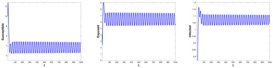
Figure 1. When $I_m=10$, the time series of the state variables $S\left(t\right)$, $E\left(t\right)$, and $I\left(t\right)$ for System (5) with $I_m=10$ and $\epsilon =0$ (no control). As the delay $\tau$ exceeds the critical value ${\tau }_0=8.6$, a Hopf bifurcation occurs, leading to the emergence of stable periodic oscillations.

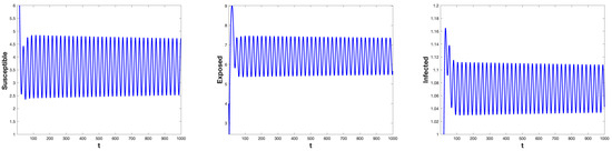
Figure 2. When $I_m=4$, the time series of the state variables $S\left(t\right)$, $E\left(t\right)$, and $I\left(t\right)$ for System (5) with $I_m=4$ and $\epsilon =1$ (under control). A Hopf bifurcation occurs at $\tau ={\tau }_0=3.5$, resulting in the formation of a stable limit cycle.

4. Sliding Mode Dynamic Behaviors

4.1. The Existence of Sliding Mode

In this section, we aim to examine the dynamics of the sliding mode of System (8) by first confirming its existence. Note $I\left(t\right)=I_m$ on $F_s$, and calculate

$$\begin{array}{cc}\hfill ⟨n,g_1⟩=& ⟨\left[\begin{array}{c}0\\ 0\\ 1\end{array}\right], \left[\begin{array}{c}\mathrm{\Lambda }-\beta S(t-\tau )I(t-\tau )-\mu S\left(t\right)\\ \beta S(t-\tau )I(t-\tau )-({\alpha }_1+\mu )E\left(t\right)\\ {\alpha }_{1}E\left(t\right)-({\alpha }_2+\mu +\delta )I\left(t\right)\end{array}\right]⟩\hfill \\ \hfill =& {\alpha }_{1}E\left(t\right)-({\alpha }_2+\mu +\delta )I_m,\hfill \end{array}$$

and

$$\begin{array}{cc}\hfill ⟨n,g_2⟩=& ⟨\left[\begin{array}{c}0\\ 0\\ 1\end{array}\right], \left[\begin{array}{c}\mathrm{\Lambda }-\beta S(t-\tau )I(t-\tau )-\mu S\left(t\right)\\ \beta S(t-\tau )I(t-\tau )-({\alpha }_1+\mu )E\left(t\right)\\ {\alpha }_{1}E\left(t\right)-({\alpha }_2+\mu +\delta +\gamma )I\left(t\right)\end{array}\right]⟩\hfill \\ \hfill =& {\alpha }_{1}E\left(t\right)-({\alpha }_2+\mu +\delta +\gamma )I_m.\hfill \end{array}$$

From $⟨n,g_1⟩>0$ and $⟨n,g_2⟩<0$, one gets

$$\begin{array}{cc}\hfill & ⟨n,g_1⟩>0,E>{\displaystyle \frac{({\alpha }_2+\mu +\delta )I_m}{{\alpha }_1}}:=E_1,\hfill \\ \hfill & ⟨n,g_2⟩<0,E<{\displaystyle \frac{({\alpha }_2+\mu +\delta +\gamma )I_m}{{\alpha }_1}}:=E_2.\hfill \end{array}$$

The sliding domain $G\subset F_s$ is defined as follows

$$G\triangleq \left\{(S,E,I)\in F_s:S\ge 0,E_1\left(I_m\right)<E<E_2\left(I_m\right),I=I_m\right\}.$$

Furthermore, we employ the Utkin equivalent control method [23] to derive the sliding mode equations within the specified region G. From $\sigma \left(I_m\right)=I\left(t\right)-I_m$ and $\mathrm{d}\sigma /\mathrm{d}t=0$, where

$$\begin{array}{c}\hfill {\displaystyle \frac{\mathrm{d}\sigma \left(t\right)}{\mathrm{d}t}}={\displaystyle \frac{\mathrm{d}I\left(t\right)}{\mathrm{d}t}}={\alpha }_{1}E\left(t\right)-({\alpha }_2+\mu +\delta )I\left(t\right)-\epsilon \gamma I\left(t\right)=0.\end{array}$$

(18)

The resolution of System (18) with respect to the variable $\epsilon$ results in the following outcome

$$\epsilon \left(I_m\right)={\displaystyle \frac{{\alpha }_{1}E\left(t\right)-({\alpha }_2+\mu +\delta )I_m}{\gamma I_m}}.$$

(19)

By substituting System (19) into System (5), the dynamics of the sliding mode within G can be expressed through the subsequent differential equations

$$\left\{\begin{array}{cc}\hfill {\displaystyle \frac{\mathrm{d}S\left(t\right)}{\mathrm{d}t}}=& \mathrm{\Lambda }-\beta S(t-\tau )I_m-\mu S\left(t\right),\hfill \\ \hfill {\displaystyle \frac{\mathrm{d}E\left(t\right)}{\mathrm{d}t}}=& \beta S(t-\tau )I_m-({\alpha }_1+\mu )E\left(t\right),\hfill \\ \hfill {\displaystyle \frac{\mathrm{d}I\left(t\right)}{\mathrm{d}t}}=& 0.\hfill \end{array}\right.$$

(20)

Lemma 1.

The uniqueness and positivity of a pseudo-equilibrium $E_p^{*}=(S_p,E_p,I_m)$ for the sliding mode in System (20) is assured, and $E_p^{*}\in G$.

Proof. 

Let $\mathrm{d}S\left(t\right)/\mathrm{d}t=0$, one gets

$$\begin{array}{cc}\hfill S_p=& {\displaystyle \frac{\mathrm{\Lambda }}{\beta I_m+\mu }},\hfill \\ \hfill E_p=& {\displaystyle \frac{\mathrm{\Lambda }\beta I_m}{(\beta I_m+\mu )({\alpha }_1+\mu )}}.\hfill \end{array}$$

If $E_p^{*}\in G\in F_s$ hold, System (5) has pseudo-equilibrium $({\displaystyle \frac{\mathrm{\Lambda }}{\beta I_m+\mu }},{\displaystyle \frac{\mathrm{\Lambda }\beta I_m}{(\beta I_m+\mu )({\alpha }_1+\mu )}},I_m)$. □

Next, we examine the local asymptotic stability of $E_p^{*}$ and present the following theorem. From System (20), the characteristic equation is given

$${\lambda }^2+j_1\lambda +j_2+(j_3\lambda +j_4)e^{-\lambda \tau }=0,$$

(21)

where

$$j_1=2\mu +{\alpha }_1,j_2=\mu ({\alpha }_1+\mu ),j_3=\beta I_m,j_4=\mu \beta I_m.$$

After establishing the sliding mode domain and identifying the pseudo-equilibrium point in System (5), we will proceed to demonstrate the stability of this point as it asymptotically converges under the specific condition where ${\tau }_1=0$.

Theorem 5.

If $\tau =0$, the unique pseudo equilibrium $E_p^{*}$ of System (5) is locally asymptotically stable.

Given that the proof methodology aligns closely with that of Theorem 2, the proof will be excluded from this discussion.

For $\tau >0$, assume that System (21) has a pair of purely imaginary roots $\lambda =i\omega$, we have

$$\left\{\begin{array}{c}-{\omega }^2+j_2=-j_3\omega sin\omega \tau -j_{4}cos\omega \tau ,\hfill \\ j_1\omega =-j_3\omega cos\omega \tau +j_{4}sin\omega \tau .\hfill \end{array}\right.$$

(22)

Add the squares to get

$${\omega }^4+(j_1^2-2j_2-j_3^2){\omega }^2+j_2^2-j_4^2=0,$$

(23)

let ${\omega }_1^2=z$, thus we have

$$f\left(z\right)=z^2+(j_1^2-2j_2-j_3^2)z+j_2^2-j_4^2=0.$$

(24)

According to System (22), we have

$$cos\omega \tau ={\displaystyle \frac{(j_4-j_1{j}_3){\omega }^2-j_2{j}_4}{j_3^2{\omega }^2+j_4^2}}.$$

Assuming that System (22) has positive root ${\omega }_k$, then

$${\tau }_k^j={\displaystyle \frac{1}{{\omega }_k}}\left\{arccos{\displaystyle \frac{(j_4-j_1{j}_3){\omega }^2-j_2{j}_4}{j_3^2{\omega }^2+j_4^2}}+2j\pi \right\}.$$

Let $\lambda \left(\tau \right)=\alpha \left(\tau \right)+i\omega \left(\tau \right)$ be the root of System (21) near $\tau ={\tau }_k^{\left(j\right)}$ statifying $\alpha ({\tau }_k^{\left(j\right)})=0$, $\omega ({\tau }_k^{\left(j\right)})={\omega }_k$, then the subsequent transversality condition is satisfied. Differentiating System (21) with respect to $\tau$, we get

$$\begin{array}{cc}\hfill ({\displaystyle \frac{d\left(Re\lambda \right(\tau \left)\right)}{d\tau }}{)}^{-1}=& Re\left\{{\displaystyle \frac{{\lambda }^2-j_2}{-{\lambda }^2({\lambda }^2+j_1\lambda +j_2)}}+{\displaystyle \frac{j_4}{-{\lambda }^2(j_3\lambda +j_4)}}\right\}\hfill \\ \hfill =& {\displaystyle \frac{{\omega }^4-j_2^2}{{\omega }^2[{(-{\omega }^2+j_1)}^2+j_2^2{\omega }^2]}}+{\displaystyle \frac{j_4^2}{{\omega }^2(j_4^2+j_3^2{\omega }^2)}}\hfill \\ \hfill =& {\displaystyle \frac{f^{\prime }\left(z_k\right)}{K^{*}}}\hfill \end{array}$$

where $K^{*}=j_4^2+j_3^2{\omega }^2$. Therefore,

$$sign{\left\{{\displaystyle \frac{\mathrm{d}\left(Re\right(\lambda \left(\tau \right)\left)\right)}{\mathrm{d}\tau }}\right\}}_{\tau ={\tau }_k^j}=sign\left\{{\displaystyle \frac{1}{K^{*}}}{f}^{\prime }\left(z_k\right)\right\}=sign\left[f^{\prime }\left(z_k\right)\right]\ne 0.$$

(25)

As the bifurcation parameter varies, the pseudo-equilibrium $E_p^{*}$ exhibits varying stability characteristics. We now present Theorem 6 to illustrate this situation.

Theorem 6.

Assuming that $f^{\prime }\left(z\right)\ne 0$, the following statements are true:

(i) 

The pseudo-equilibrium $E_p^{*}$ for System (20) is asymptotically stable for $\tau \in [0,{\tau }_0)$.

(ii) 

For $\tau >{\tau }_0$, pseudo-equilibrium $E_p^{*}$ becomes unstable.

(iii) 

For $\tau ={\tau }_k^j$ with $(0\le k\le \tilde{k}$ and $j\in N_0$), bifurcated periodic solutions are generated, which appear as spatially non-uniform periodic orbits at the $E_p^{*}$ point and are unstable. Conversely, when $\tau ={\tau }_0^j$ for $j\in N_0$, the bifurcating periodic solutions are spatially homogeneous periodic orbits at $E_p^{*}$.

4.2. Numerical Simulations of Sliding Mode

When the threshold $I_m$ takes different values, the system will exhibit different dynamics. The parameter settings remain the same as in Section 3, and the theory is verified through numerical simulations in the following.

Case 1: $E_1^{*}$ is a regular equilibrium, and $E_2^{*}$ is a virtual equilibrium.

When $E_1^{*}$ is regular equilibrium and $E_2^{*}$ is virtual equilibrium, then $I_1<I_m$ and $I_2<I_m$. In this case, both equilibria are situated on the same side of the $I_m$ plane, specifically within the region $F_1$. Consequently, it can be concluded that $E_1^{*}$ is capable of attaining stability. In Figure 3, $E_1^{*}\in F_1$, which stabilizes at $I_m=10$, the possible trajectories of the graph are shown: Trajectories starting in the $F_1$ region will converge to $E_1^{*}$ as $t\to \infty$ bumps and slides down the sliding domain; trajectories with the initial point in the $F_2$ region will pass through the manifold $F_s$, then enter the $F_1$ region and eventually converge to $E_1^{*}$; trajectories starting in the $F_1$ or $F_2$ region will bump and slide to the boundary of the sliding domain $F_s$ and then converge to $E_1^{*}$, the boundary of the sliding domain $F_s$ and then converge to $E_1^{*}$.

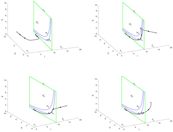
Figure 3. The phase portrait and sliding mode domain $G\subset F_s$ are presented for the scenario in which $E_1^{*}$ represents a regular equilibrium point, while $E_2^{*}$ corresponds to a virtual equilibrium, with the parameter $I_m=10$. Trajectories initiating within regions $F_1$ or $F_2$ exhibit convergence towards $E_1^{*}$, with certain trajectories entering the sliding domain G before convergence.

Case 2: $E_2^{*}$ is a regular equilibrium, and $E_1^{*}$ is a virtual equilibrium.

When $E_1^{*}$ is virtual equilibrium and $E_2^{*}$ is regular equilibrium, then $I_1>I_m$ and $I_2>I_m$. In this case, both equilibria are situated in the region $F_2$. In Figure 4, $E_2^{*}\in F_2$, which stabilizes at $I_m=4$, the possible trajectories of the graph are shown: Trajectories starting in the $F_1$ region will converge to $E_2^{*}$ as $t\to \infty$ bumps and slides down the sliding domain; trajectories with the initial point in the $F_1$ region will pass through the manifold $F_s$, then enter the $F_2$ region and eventually converge to $E_2^{*}$; trajectories starting in the $F_1$ or $F_2$ region will bump and slide to the boundary of the sliding domain $F_s$ and then converge to $E_2^{*}$, the boundary of the sliding domain $F_s$ and then converge to $E_2^{*}$.

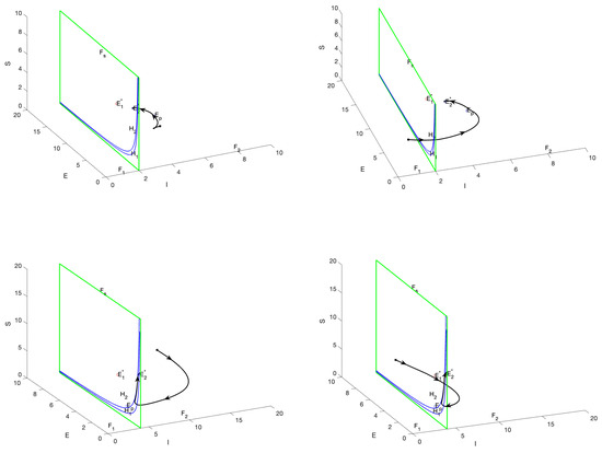
Figure 4. The phase portrait and sliding mode domain $G\subset F_s$ are presented for the scenario in which $E_2^{*}$ represents a regular equilibrium point, while $E_1^{*}$ is a virtual equilibrium, with the parameter $I_m=4$. Trajectories originating from both regions ultimately converge to $E_2^{*}$, thereby illustrating the stability of the regular equilibrium.

Case 3: $E_1^{*}$ and $E_2^{*}$ are virtual equilibria.

When $E_1^{*}$ and $E_2^{*}$ are virtual equilibria, then $I_1>I_m$ and $I_2<I_m$. $E_p\in F_S$ stabilizes at $I_m=7$. Figure 5 shows the possible trajectories: A trajectory whose initial condition lies in the $F_1$ region will converge to $E_p$ as $t\to \infty$; a trajectory that starts in the $F_2$ region will pass through the manifold $F_s$ and then into the $F_1$ region, finally converging to $E_p$; a trajectory whose initial condition lies in the $F_1$ region will hit and slide downward on $G_s$ and then converge to $E_p$. When $I_m=7$, $E_1^{*}$ and $E_2^{*}$ are virtual equilibria. According to the calculation, ${\tau }_0=4.1$. As $\tau$ increases, System (5) will exhibit a bifurcation of periodic solutions with the bifurcation of regular equilibria around ${\tau }_0$, as shown in Figure 6.

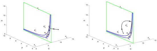
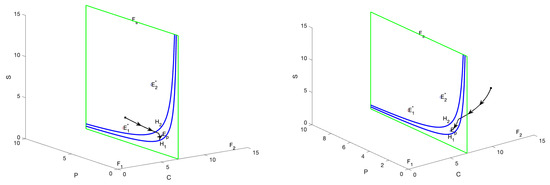
Figure 5. The phase portrait illustrates the scenario in which both $E_1^{*}$ and $E_2^{*}$ represent virtual equilibria, with the parameter $I_m=7$. The trajectories are observed to converge toward the pseudo-equilibrium $E_p^{*}$ located within the sliding region G, thereby demonstrating the dynamics characteristic of the sliding mode.

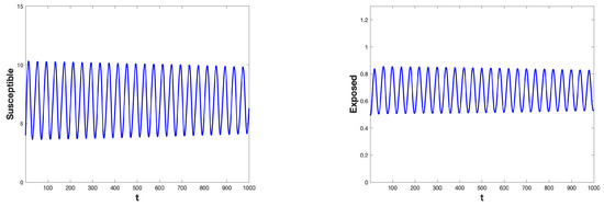
Figure 6. The time series of $S\left(t\right)$, $E\left(t\right)$, and $I\left(t\right)$ are presented for the parameter values $I_m=7$ and $\epsilon =0$, illustrating a Hopf bifurcation occurring at the critical delay $\tau ={\tau }_0=4.1$. As the delay parameter $\tau$ increases beyond this critical value, the system undergoes a transition from a stable equilibrium state to a periodic oscillatory solution.

The infection rate $\beta$ and the progression rate ${\alpha }_1$ have been identified as the parameters exerting the most significant positive impact on the basic reproduction number, $R_1$. Specifically, an increase in either $\beta$, which denotes the rate at which susceptible individuals become infected, or ${\alpha }_1$, representing the rate at which exposed individuals progress to an infectious state, results in a significant increase in $R_1$. This escalation consequently facilitates enhanced transmission of malaria. Figure 7 illustrates the relevant content.

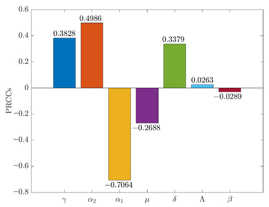
Figure 7. PRCC were calculated to assess the relationship between the basic reproduction number $R_1$ and the model parameters.

5. Conclusions

This paper investigates a delayed malaria model incorporating threshold control strategies. We first establish the local asymptotic stability of the positive equilibrium point and demonstrate the occurrence of Hopf bifurcation at the critical delay value $\tau ={\tau }_0$ (with the system being locally asymptotically stable when $\tau =0$). Furthermore, by employing the Utkin equivalent control method, we analyze the sliding mode domain and corresponding dynamics when the infected population reaches the threshold level $I=I_m$. Our analytical results demonstrate that the proposed threshold control strategy can effectively maintain the infection level below predetermined target values, providing a theoretical foundation for malaria control interventions.

Previously, the Filippov system was mostly used in HIV models [14] or predation systems [12], with very few related studies in the field of malaria. This model triggers “medical” intervention through the threshold $I_m$. The non-smooth characteristics that are more in line with actual prevention and control fill the research gap of the dynamics of discontinuous intervention for malaria. Quantify the influence of time delay on Hopf bifurcation, provide the analytical expression of the critical time delay $\tau$, and in combination with threshold control, clarify the rule that the smaller the threshold, the lower the tolerance of time delay, providing a quantitative basis for the selection of intervention timing. In terms of application innovation: Verify the effectiveness of threshold control through sliding mode dynamics analysis; The Utkin equivalent control method was used to derive the sliding mode domain G and the pseudo-equilibrium point $E_p^{*}$. It was proved that when $I=I_m$, the system could stably remain within the sliding mode domain, preventing the number of infections from exceeding the threshold and solving the problem of inability to dynamically adjust the intervention intensity in the traditional continuous model, providing a new perspective for the precise prevention and control of malaria.

This study also has some limitations. Firstly, the model only considers a single discrete time delay and does not explore the multiple time delays or distributed time delays that may exist in malaria transmission. Secondly, although the parameters of the model are based on literature, large-scale fitting and verification have not yet been carried out for the real epidemic data of specific regions. Future research will focus on constructing more general models with continuous distributed time delays and introducing factors such as age structure, spatial heterogeneity, and multi-strain competition to more comprehensively reveal the complex dynamic behavior of malaria transmission and provide a stronger theoretical basis for formulating precise prevention and control strategies.

References

- Mandal, S.; Sarkar, R.R.; Sinha, S. Mathematical models of malaria review. Malar. J. 2011, 10, 202. [Google Scholar] [CrossRef]
- Koella, J.C. On the use of mathematical models of malaria transmission. Acta Trop. 1991, 49, 1–25. [Google Scholar] [CrossRef] [PubMed]
- Dietz, K.; Molineaux, L.; Thomas, A. A malaria model tested in the African savannah. Bull. World Health Organ. 1974, 50, 347. [Google Scholar] [PubMed]
- Lunde, T.M.; Bayoh, M.N.; Lindtjørn, B. How malaria models relate temperature to malaria transmission. Parasites Vectors 2013, 6, 20. [Google Scholar] [CrossRef] [PubMed]
- Gao, D.; Ruan, S. A multipatch malaria model with logistic growth populations. Siam J. Appl. Math. 2012, 72, 819–841. [Google Scholar] [CrossRef]
- Savi, M.K. An overview of malaria transmission mechanisms, control, and modeling. Med Sci. 2022, 11, 3. [Google Scholar] [CrossRef]
- Talapko, J.; Škrlec, I.; Alebić, T.; Jukić, M.; Včev, A. Malaria: The past and the present. Microorganisms 2019, 7, 179. [Google Scholar] [CrossRef]
- Duffy, P.E.; Gorres, J.P.; Healy, S.A.; Fried, M. Malaria vaccines: A new era of prevention and control. Nat. Rev. Microbiol. 2024, 22, 756–772. [Google Scholar] [CrossRef]
- Wang, A.; Xiao, Y.; Zhu, H. Dynamics of a Filippov epidemic model with limited hospital beds. Math. Biosci. Eng. 2017, 15, 739–764. [Google Scholar] [CrossRef]
- Zhang, Y.; Song, P. Dynamics of the piecewise smooth epidemic model with nonlinear incidence. Chaos Solitons Fractals 2021, 146, 110903. [Google Scholar] [CrossRef]
- Dong, C.; Xiang, C.; Xiang, Z.; Yang, Y. Global dynamics of a Filippov epidemic system with nonlinear thresholds. Chaos Solitons Fractals 2022, 163, 112560. [Google Scholar] [CrossRef]
- Ruan, S.; Xiao, D.; Beier, J.C. On the delayed Ross–Macdonald model for malaria transmission. Bull. Math. Biol. 2008, 70, 1098–1114. [Google Scholar] [CrossRef] [PubMed]
- Rafiq, M.; Ahmadian, A.; Raza, A.; Baleanu, D.; Ahsan, M.S.; Sathar, M.H.A. Numerical control measures of stochastic malaria epidemic mode. Comput. Mater. Contin. 2020, 65, 33–51. [Google Scholar]
- Bastaki, H.; Carter, J.; Marston, L.; Cassell, J.; Rait, G. Time delays in the diagnosis and treatment of malaria in non-endemic countries: A systematic review. Travel Med. Infect. Dis. 2018, 21, 21–27. [Google Scholar] [CrossRef]
- Shuai, Z.; van den Driessche, P. Global stability of infectious disease models using Lyapunov functions. SIAM J. Appl. Math. 2013, 73, 1513–1532. [Google Scholar] [CrossRef]
- Zhang, X.; Zhao, H. Dynamics analysis of a delayed reaction-diffusion predator-prey system with non-continuous threshold harvesting. Math. Biosci. 2017, 289, 130–141. [Google Scholar]
- Pei, Y.; Shen, N.; Zhao, J.; Yu, Y.; Chen, Y. Analysis and simulation of a delayed HIV model with reaction–diffusion and sliding control. Math. Comput. Simul. 2023, 212, 382–405. [Google Scholar] [CrossRef]
- Shi, D.; Ma, S.; Zhang, Q. Sliding mode dynamics and optimal control for HIV model. Math. Biosci. Eng. 2023, 20, 7273–7297. [Google Scholar] [CrossRef]
- Al-Arydah, M.; Smith, R. Controlling malaria with indoor residual spraying in spatially heterogeneous environments. Math. Biosci. Eng. 2011, 8, 889–914. [Google Scholar]
- Liu, J.; Yang, B.; Cheung, W.K.; Yang, G. Malaria transmission modelling: A network perspective. Infect. Dis. Poverty 2012, 1, 11. [Google Scholar]
- Ho, M.T.; Datta, A.; Bhattacharyya, S.P. An elementary derivation of the Routh-Hurwitz criterion. IEEE Trans. Autom. Control 1998, 43, 405–409. [Google Scholar]
- Willems, J.L. Stability Theory of Dynamical Systems; Springer: Berlin/Heidelberg, Germany, 1970. [Google Scholar]
- Utkin, V.I. Sliding Modes in Control and Optimization; Springer: Berlin/Heidelberg, Germany, 2013. [Google Scholar]
Disclaimer/Publisher’s Note: The statements, opinions and data contained in all publications are solely those of the individual author(s) and contributor(s) and not of MDPI and/or the editor(s). MDPI and/or the editor(s) disclaim responsibility for any injury to people or property resulting from any ideas, methods, instructions or products referred to in the content. |
© 2025 by the authors. Licensee MDPI, Basel, Switzerland. This article is an open access article distributed under the terms and conditions of the Creative Commons Attribution (CC BY) license (https://creativecommons.org/licenses/by/4.0/).