Determining Convergence for Expected Improvement-Based Bayesian Optimization

Abstract

Bayesian optimization routines may have theoretical convergence results, but determining whether a run has converged in practice can be a subjective task. This paper provides a framework inspired by statistical process control for monitoring an optimization run for convergence. The maximum Expected Improvement (EI) tends to decrease during an optimization run, but decreasing EI is not sufficient for convergence. We consider both a decrease in EI as well as local stability of the variance in order to assess for convergence. The EI process is made more numerically stable through an expected log-normal approximation. An Exponentially Weighted Moving Average control chart is adapted for automated convergence analysis, which allows assessment of stability of both the EI and its variance. The success of the methodology is demonstrated on several examples.

1. Introduction

Bayesian optimization aims to find a global optimum of a complex function that may not be analytically tractable and where derivative information may not be readily available [1,2]. A common application is for computer simulation experiments [3]. Because each function evaluation may be expensive, one wants to terminate the optimization algorithm as early as possible. However, for complex simulators, the response surface may be ill-behaved, and optimization routines can easily become trapped in a local mode, so one needs to run the optimization sufficiently long to achieve a robust solution. So far, there has been little work on assessing convergence for Bayesian optimization. In this paper, we provide an automated method for determining the convergence of surrogate model-based optimization by bringing in elements of statistical process control.

Among the wide variety of Bayesian optimization approaches, we focus on those that are based on a statistical surrogate model, such as a Gaussian process [4]. We further focus on approaches based on Expected Improvement (EI) [5], although our methods are generalizable for other acquisition functions.

Recently, some stopping criteria for Bayesian optimization have been developed around the concept of regret [6,7,8]. These methods theoretically capture the stochastic nature of Bayesian optimization convergence well but can be expensive to evaluate, especially when problems require surrogate models that are more flexible than standard GPs. This paper takes a completely different approach inspired by Statistical Process Control (SPC). An alternative to regret that has been hinted at in the literature is that monitoring EI directly could be used to assess convergence [9]. This would allow for the use of more flexible surrogate models. The use of the improvement distribution for identifying global convergence was considered in [10]. The basic idea is that convergence should occur when the surrogate model produces low expectations for discovering a new optimum; that is to say, globally small EI values should be associated with convergence of the algorithm. Thus, a simplistic stopping rule might first define some lower EI threshold, then claim convergence upon the first instance of an EI value falling below this threshold, as seen in [11]. This use of EI as a convergence criterion is analogous to other standard convergence identification methods in numerical optimization (e.g., the vanishing step sizes of a Newton–Raphson algorithm). However, applying this same threshold strategy to the convergence of Bayesian optimization has not yet been adequately justified. In fact, this use of EI ignores the nature of the EI criterion as a random variable, and oversimplifies the stochastic nature of convergence in this setting. Thus, it is no surprise that this treatment of the EI criterion can result in an inconsistent stopping rule as demonstrated in Figure 1. By extending this approach to capture the stochastic nature of Bayesian optimization convergence, we propose a relatively simple and computationally efficient method for stopping Bayesian optimization.

Because EI is strictly positive but decreasingly small, we find it more productive to work on the log scale, using a log-normal approximation to the improvement distribution to generate a more appropriate convergence criterion, as described in Section 3.2. Figure 1 represents three series of the Expected Log-normal Approximation to the Improvement (ELAI) values from three different optimization problems. We will demonstrate later in this paper that convergence is established near the end of each of these series. These three series demonstrate the kind of diversity observed among various ELAI convergence behaviors and illustrate the difficulty in assessing convergence. In the left-most panel, optimization of the Rosenbrock test function results in a well-behaved series of ELAI values, demonstrating a case in which the simple threshold stopping rule can accurately identify convergence. However, the center panel (the Lockwood problem described in Section 4.4) demonstrates a failure of the threshold stopping rule, as this ELAI series contains much more variance, and thus small ELAI values are observed quite regularly. In the Lockwood example, a simple threshold stopping rule could falsely claim convergence within the first 50 iterations of the algorithm. The large variability in ELAI values with occasional large values indicates that the optimization routine sometimes briefly settles into a local minimum but is still exploring and is not yet convinced that it has found a global minimum. This optimization run appears to have converged only after the larger ELAI values stop appearing and the variability has decreased. Thus one might ask if a decrease in variability, or small variability, is a necessary condition for convergence. The right-most panel (the Rastrigin test function) shows a case where convergence occurs by meeting the threshold level, but where variability has increased, demonstrating that a decrease in variability is not a necessary condition.

Since the Improvement function is itself random, attempting to set a lower threshold bound on the EI, without consideration of the underlying EI distribution through time, over-simplifies the dynamics of convergence in this setting. Instead, we propose taking a perspective analogous to SPC, where a stochastic series is monitored for consistency of the distribution of the most recently observed values. This approach is taking into account both the values of the process and the variability among those values, looking for a region of stability jointly in value and variability as a sign that the optimization is no longer making progress. In the next section, we review the surrogate model approach and the use of EI for optimization. In Section 3, we discuss our inspiration from SPC and how we construct our convergence chart. Section 4 provides synthetic and real examples. A simulation experiment is used in Section 5 to compare the SPC approach to existing approaches, and then we provide some conclusions in the final section.

2. Bayesian Optimization via Expected Improvement

Bayesian optimization attempts to solve problems of the form

$$x^{*}=\underset{x\in \mathcal{X}}{argmin}f\left(x\right),$$

(1)

where $x^{*}$ is the optimum, f is an objective function (often not available in analytical form), and $x\in \mathcal{X}\subset {\mathbb{R}}^d$. $\mathcal{X}$ may be defined via constraints. Without loss of generality, we frame all optimizations as minimizations in this paper, as maximization can be recovered by minimizing the negative of the function. Bayesian optimization proceeds by iteratively developing a statistical surrogate model of the objective function f and using predictions from the statistical surrogate to choose the next point to evaluate based on some criterion. A common choice of surrogate model is the Gaussian process (GP) [3,12], as it combines flexibility with smoothness.

In many cases, the assumption of a globally smooth f with a homogeneous uncertainty structure can provide an effective and parsimonious model. However, in other problems, f may have sharp boundaries, f may show different levels of smoothness across its domain, or numerical simulators may have variable stability in portions of the domain. In this paper, we use treed Gaussian processes [13], a generalization of a standard GP that uses treed partitioning of the domain, fitting separate hierarchically linked stationary GP surfaces to separate portions of f via a reversible jump Markov Chain Monte Carlo algorithm and averaging over the full parameter space to provide smooth predictions except where the data call for a discontinuous prediction. The treed GP surrogate model is implemented here using the R package tgp [14], version 2.4, to sample from the GP and improvement predictive distributions. While treed GPs provide additional modeling flexibility, we emphasize that the approach of this paper can be applied to standard GPs as well as any surrogate model that provides both predictions and predictive uncertainty.

2.1. Expected Improvement

Bayesian optimization requires an acquisition function that guides the choice of a new function evaluation at each iteration. There are a wide variety of suggestions for acquisition functions. A large family of options is based on Expected Improvement. The EI criterion predicts how likely a new minimum is to be observed, at new locations of the domain, based upon the predictive distribution of the surrogate model. EI is built upon the improvement function [9]:

$$\mathrm{I}\left(\mathit{x}\right)=max\left\{\left(f_{min}-f\left(\mathit{x}\right)\right),0\right\},$$

(2)

where $f_{min}$ is the smallest function value observed so far. EI is the expectation of the improvement function with respect to the posterior predictive distribution of the surrogate model, $\mathbb{E}\left[\mathrm{I}\left(\mathit{x}\right)\right]$. EI rewards candidates both for having a low predictive mean, as well as high uncertainty (where the function has not been sufficiently explored), thus balancing global exploration and local exploitation. By definition, the improvement function is always non-negative and the posterior predictive $\mathbb{E}\left[\mathrm{I}\left(\mathit{x}\right)\right]$ is strictly positive. The EI criterion is available in closed form for a stationary GP. For other models, the EI criterion can be quickly estimated using Monte Carlo posterior predictive samples at given candidate locations.

2.2. Optimization Procedure

Optimization can be viewed as a sequential design process, where locations are selected for evaluation on the basis of how likely they are to decrease the objective function, i.e., based on the EI. Optimization begins by initially collecting a set, $\mathit{X}$, of locations to evaluate the true function, f, to obtain an initial fit of the statistical surrogate model, using $f\left(\mathit{X}\right)$ as observations of the true function. Based on the surrogate model, a set of candidate points, $\tilde{\mathit{X}}$, are selected from the domain, and the EI criterion is calculated among these points. The candidate point that has the highest EI is then chosen as the best candidate for a new minimum and thus is added to $\mathit{X}$. The objective function is evaluated at this new location, and the surrogate model is refit using the updated $f\left(\mathit{X}\right)$. The optimization procedure continues in this way until convergence. Figure 2 provides pseudo-code for this type of optimization process. The key contribution of this paper is an automated method for checking convergence, which we develop in the next section.

3. Exponentially Weighted Moving Average (EWMA) Convergence Chart

3.1. Statistical Process Control

In Shewhart’s seminal book [15] on the topic of control in manufacturing, Shewhart explains that a phenomenon is said to be in control when, “through the use of past experience, we can predict, at least within limits, how the phenomenon may be expected to vary in the future.” This notion provides an instructive framework for thinking about convergence because it offers a natural way to consider the distributional characteristics of the EI as a proper random variable. In its most simplified form, SPC considers an approximation of a statistic’s sampling distribution as repeated sampling occurs in time. Thus, Shewhart can express his idea of control as the expected behavior of random observations from this sampling distribution. For example, an $\overline{x}$-chart tracks the mean of repeated samples (all of size n) through time so as to expect the arrival of each subsequent mean in accordance with the known or estimated sampling distribution for the mean, ${\overline{x}}_j\sim N\left(\mu ,{\displaystyle \frac{{\sigma }^2}{n}}\right)$. By considering confidence intervals on this sampling distribution we can draw explicit boundaries (i.e., control limits) to identify when the process is in control and when it is not. Observations violating our expectations (falling outside of the control limits) indicate an out of control state. Since neither $\mu$ nor ${\sigma }^2$ are typically known, it is common to collect an initial set of data from which point estimates of $\mu$ and ${\sigma }^2$ may establish an initial standard for control that is further refined as the process proceeds. This logic relies upon the typical asymptotic results of the central limit theorem (CLT), and care should be taken to verify the relevant assumptions required.

It is important to note that we are not performing traditional SPC in this context, as the EI criterion will be stochastically decreasing as an optimization routine proceeds. Only when convergence is reached will the EI series look approximately like an in control process. Thus, our perspective is completely reversed from the traditional SPC approach—we start with a process that is out of control, and we determine convergence when the process stabilizes and becomes locally in control. An alternative way to think about our approach is to consider performing SPC backwards in time on our EI series. Starting from the most recent EI observations and looking back, we declare convergence if the process starts in control and then becomes out of control. This pattern generally appears only when the optimization has progressed and reached a local mode without other prospects for a global mode. If the optimization were still proceeding, then the EI would still be decreasing and the most recent iterations of optimization would not appear to be in control.

3.2. Expected Log-Normal Approximation to the Improvement (ELAI)

For the sake of obtaining a robust convergence criterion to track via SPC, it is important to carefully consider properties of the improvement distributions which generate the EI values. The improvement criterion is strictly positive but decreasingly small; thus, the improvement distribution is often strongly right skewed, in which case, the EI is far from normal. Additionally, this right skew becomes exaggerated as convergence approaches, due to the decreasing trend in the EI criterion. These issues naturally suggest modeling transformations of the improvement, rather than directly considering the improvement distribution on its own. One of the simplest of the many possible helpful transformations in this case would consider the log of the improvement distribution. However due to the Monte Carlo sample-based implementation of the Gaussian process, it is not uncommon to obtain at least one sample that is computationally indistinguishable from zero in double precision. Thus, simply taking the log of the improvement samples can result in numerical failure, particularly as convergence approaches, even though the quantities are theoretically strictly positive. Despite this numerical inconvenience, the distribution of the improvement samples is often very well approximated by the log-normal distribution.

We avoid the numerical issues by using a model-based approximation. With the desire to model $\mathbb{E}\left[log\mathrm{I}\right]∻N\left(\mu ,{\displaystyle \frac{{\sigma }^2}{n}}\right)$, we switch to a log-normal perspective. Recall that if a random variable $X\sim Log-N(\theta ,\varphi ),$ then another random variable Y = log(X) is distributed $Y\sim N(\theta ,\varphi )$. Furthermore, if ω and ψ are the mean and variance of a log-normal sample, respectively, then the mean, θ, and variance, ϕ, of the associated normal distribution are given by the following relation.

$$\begin{array}{ccc}\hfill \theta =\log \left({\displaystyle \frac{{\omega }^2}{\sqrt{\psi +{\omega }^2}}}\right)& & \varphi =\log \left(1+{\displaystyle \frac{\psi }{{\omega }^2}}\right).\hfill \end{array}$$

(3)

Using this relation, we do not need to transform any of the improvement samples. We compute the empirical mean and variance of the unaltered, approximately log-normal, improvement samples, then use relation (3) to directly compute ω as the Expectation under the Log-normal Approximation to the Improvement (ELAI). The ELAI value is useful for assessing convergence because of the reduced right skew of the log of the posterior predictive improvement distribution. Additionally, the ELAI serves as a computationally robust approximation of the $\mathbb{E}\left[\log \mathrm{I}\right]$ under reasonable log-normality of the improvements. Furthermore, both the $\mathbb{E}\left[\log \mathrm{I}\right]$ and ELAI are distributed approximately normally in repeated sampling. This construction allows for more consistent and accurate use of the fundamental theory on which our SPC perspective depends. We note that the approximation will be more accurate when the process is near or at convergence; the accuracy of the approximation is not critical while the process is out of control and not yet in convergence, so we only need a good approximation in the region of convergence.

3.3. Exponentially Weighted Moving Average

The Exponentially Weighted Moving Average (EWMA) control chart [16,17] elaborates on Shewhart’s original notion of control by viewing the repeated sampling process in the context of a moving average smoothing of series data. The general concept of a control chart is that it is monitoring a process that is “in control”, and it checks to see if the process changes, flagging a new point as not in control if it is outside of expectations. The expectations are based on having a stable mean and a stable variance; changes in either the mean or the variance can trigger a loss of control.

In our context, pre-convergence ELAI evaluations tend to be variable and overall decreasing, and so do not necessarily share distributional consistency among all observed values. Thus, a weighted series perspective was chosen to follow the moving average of the most recent ELAI observations while still smoothing with some memory of older evaluations. EWMA achieves this robust smoothing behavior, relative to shifting means, by assigning exponentially decreasing weights to successive points in a rolling average among all of the points of the series. Thus, the EWMA can emphasize recent observations and shift the focus of the moving average to the most recent information while still providing shrinkage towards the global mean of the series.

Let $Y_t$ be the ELAI value observed at the $t^{th}$ iteration of optimization forwards in time, such that $t\in \{1,2,3,...T\}$, where T is then the most recently completed iteration of optimization. To step backwards in time, we introduce $s=T-t+1$ to track indices scanning from the most recent iteration of optimization backwards towards the first iteration. Indexing backwards in time, let $Z_s$ be the EWMA statistic associated with $Y_s$, and progressing through the previous iterations of optimization the EWMA statistics are expressed as $Z_s=\lambda Y_s+(1-\lambda )Z_{s-1}$. To initialize the recurrence, $Z_{s=0}$ is set to the observed mean of Y over the modeled period. Here, $\lambda \in (0,1]$ is a smoothing parameter that defines the weight assigned to the most recent observation. The recursive expression of the statistic ensures that all subsequent weights geometrically decrease.

$\lambda$ is estimated by minimizing the sum of squared forecasting deviations, based on the method described in [18]. $\lambda$ is therefore automatically selected by solving:

$$\widehat{\lambda }=\underset{\lambda \in (0,1]}{argmin}\left(\sum _i{\left(Y_i-Z_i\left(\lambda \right)\right)}^2\right).$$

(4)

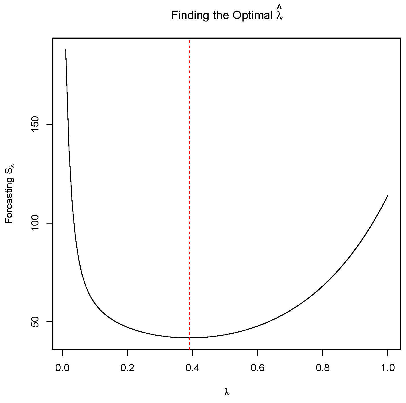
Figure 3 shows the sum of squared forecasting deviations as a function of $\lambda$. The relatively flat region around the minimum in Figure 3 demonstrates that EWMA charts can be very robust to reasonable choices of $\lambda$ for a large range of sub-optimal choices of $\lambda$ around $\widehat{\lambda }$. In fact, Figure 3 shows that for $\lambda \in [0.2,0.6]$, the sum of squared forecasting deviations stays within 10% of the minimum possible value.

Identifying convergence in this setting now requires the computation of control limits on the EWMA statistic. As in the simplified $\overline{x}$-chart, defining the control limits for the EWMA setting amounts to considering an interval on the sampling distribution of interest. In the EWMA case, we are interested in the sampling distribution of the $Z_s$. Assuming that the $Y_s$ are $i.i.d.$, then [16] show that we can write ${\sigma }_{Z_s}^2$ in terms of ${\sigma }_Y^2$.

$${\sigma }_{Z_s}^2={\sigma }_Y^2\left({\displaystyle \frac{\lambda }{2-\lambda }}\right)\left[1-{(1-\lambda )}^{2s}\right]$$

(5)

Thus, if $Y_s\stackrel{i.i.d.}{\sim }N\left(\mu ,{\displaystyle \frac{{\sigma }^2}{n}}\right)$, then the sampling distribution for $Z_s$ is $Z_s\sim N\left(\mu ,{\sigma }_{Z_s}^2\right)$. Furthermore, by choosing a confidence level through choice of a constant c, the control limits based on this sampling distribution are seen in Equation (6).

$${\mathrm{CL}}_s=\mu \pm c{\sigma }_{Z_s}=\mu \pm c{\displaystyle \frac{\sigma }{\sqrt{n}}}\sqrt{\left({\displaystyle \frac{\lambda }{2-\lambda }}\right)\left[1-{(1-\lambda )}^{2s}\right]}$$

(6)

Notice that since ${\sigma }_{Z_s}^2$ has a dependence on s, the control limits do as well. Looking back through the series brings us away from the focus of the moving average, and thus the control limits widen as $s\to \infty$, where the control limits approach $\mu \pm c\sqrt{{\displaystyle \frac{\lambda {\sigma }^2}{(2-\lambda )n}}}$.

Our aim in applying the EWMA framework in this context is to recognize the fundamental notion of control that EWMA enforces in the newly arriving EI values, as optimization proceeds. Convergence often arises as a subtle shift of the EI distribution into place. In this context, a more traditional $\overline{x}$ chart will often overlook convergence as a subtle random fluctuation, when in fact it is often this subtle signal that we aim to pick-up. EWMA is among the better techniques for recognizing such subtly shifting means [19,20], while maintaining the capability to detect abrupt shifts in mean. As convergence approaches, the newly arriving Y begin to fit into the $i.i.d.$ EWMA framework and the Z increasingly begin to fall within the EWMA control limits. EWMA’s recognition of such a controlled region in the newly arriving ELAI values indicates the notion of distributional consistency that is necessary for defining convergence for stochastic measures of convergence, such as EI.

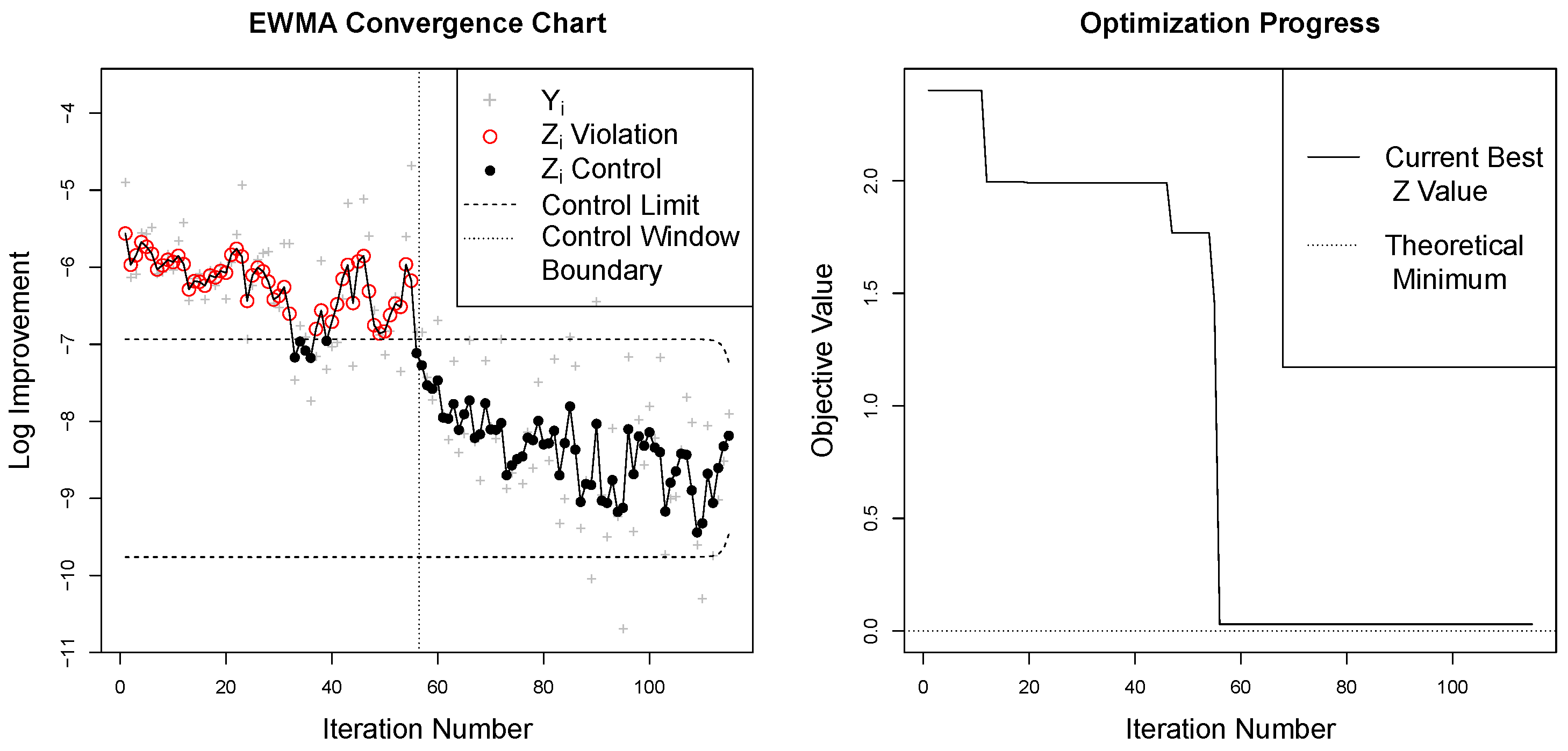
The control chart framework assumes that the $Y_s$ are $i.i.d.$ when the process is in control. We describe our approach as “inspired by Statistical Process Control” because the $Y_s$ are not actually $i.i.d.$ The early iterations of the convergence processes seen in Figure 1 certainly do not display $i.i.d.$$Y_s$. However, as the series approaches convergence, the $Y_s$ eventually do enter a state of control, see, for example, Figure 4. For these $Y_s$ at convergence, they are still not exactly $i.i.d.$, because the surrogate model variance will continue to very slightly decrease with each iteration, but an $i.i.d.$ approximation is reasonable. The realization of such a controlled region of the series defines the notion of consistency that allows for the identification of convergence.

3.4. The Control Window

The final structural feature needed to compute the EWMA convergence chart is the control window. The control window contains a fixed number, w, of the most recently observed Y (i.e., $\left\{Y_s\right|s\le w\}$). Only information from the w points currently residing inside the control window is used to calculate the control limits and $Z_0$. To assess convergence, the EWMA statistic is computed for all $Y_s$ values. Initially, the convergence algorithm is allowed to fill the control window by collecting an initial set of w ELAI observations. As a new observation arrives, the window slides to exclude the oldest observation and include the newest to maintain its definition as the w most recent observations.

The purpose of the control window is two-fold. First, it serves to dichotomize the series for evaluating subsets of the $Y_s$ for distributional consistency. Second, it offers a structural way for basing the standard for consistency (i.e., the control limits) only on the most recent and relevant information in the series.

The size of the control window, w, may vary from problem to problem based on the difficulty of optimization in each case. A reasonable way of choosing w is to consider the number of observations necessary to establish a standard of control. In this setting, w is a kind of sample size, and as such the choice of w will naturally increase as the variability in the ELAI series increases. Just as in other sample size calculations, the choice of an optimal w must consider the cost of poor inference (premature identification of convergence) associated with underestimating w, against the cost of over sampling (continuing to sample after convergence has occurred) associated with overestimating w. Providing a default choice of w is somewhat arbitrary without careful analysis of the particulars of the objective function behavior, the costs of each successive objective function evaluation, and the users’ risk tolerance to prematurely declaring convergence.

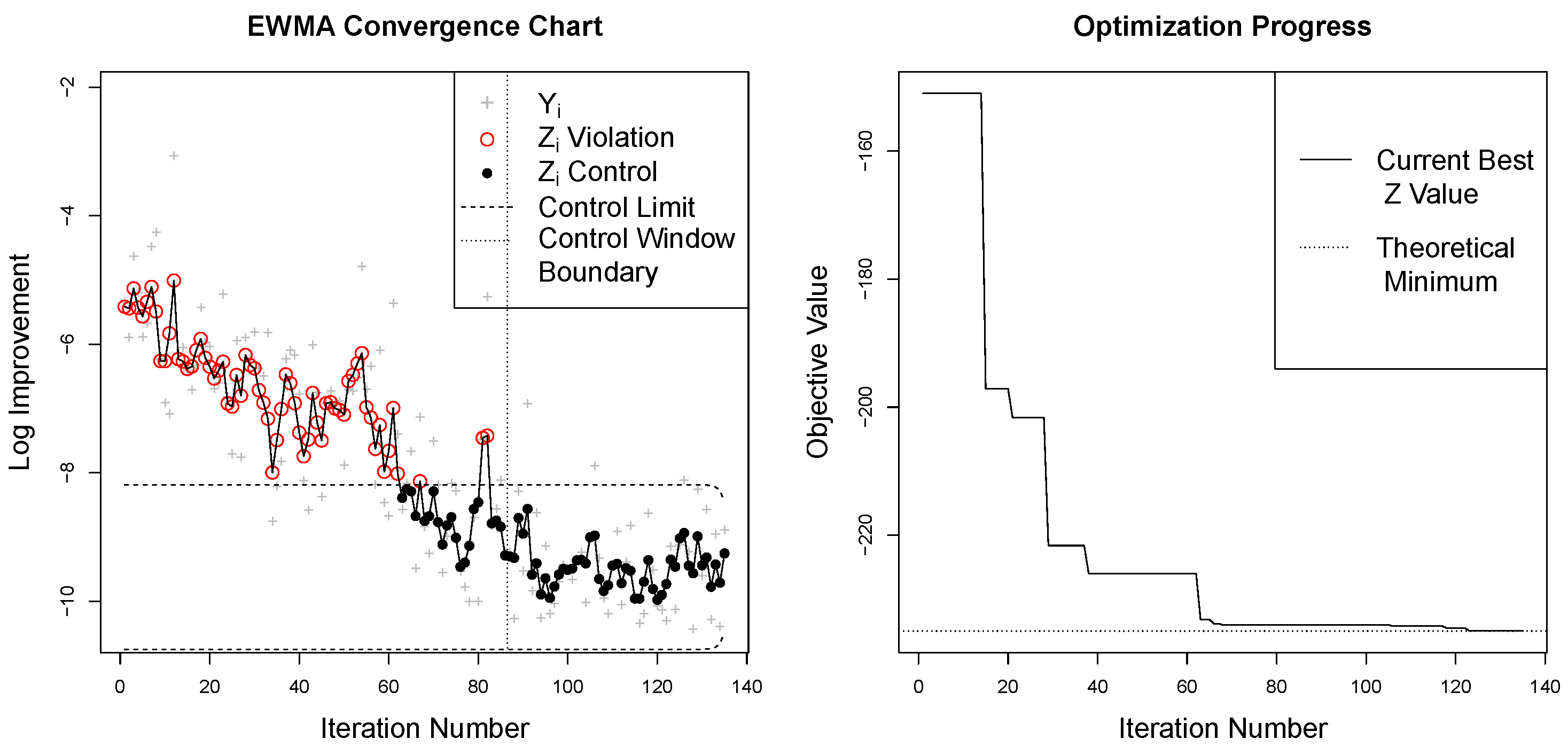
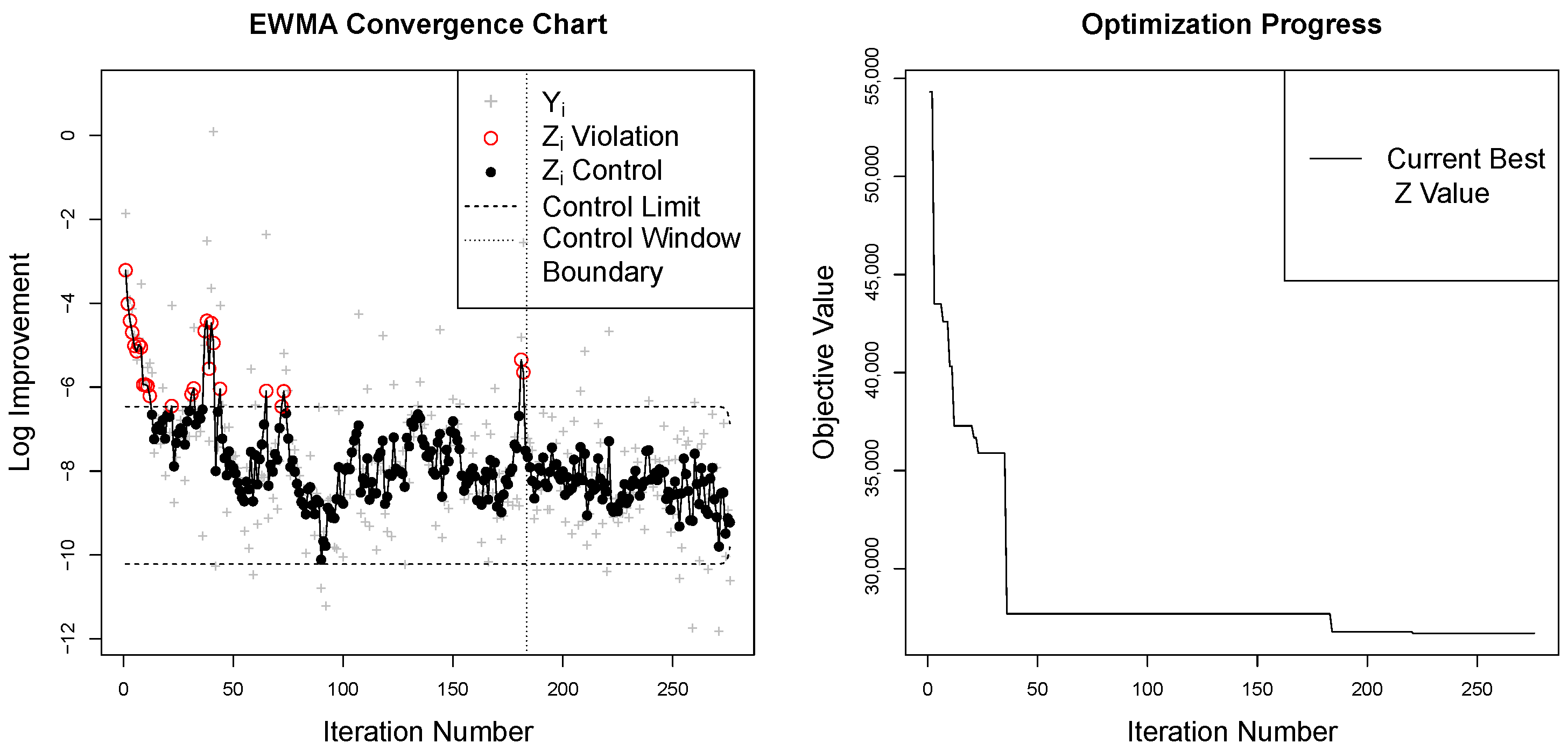
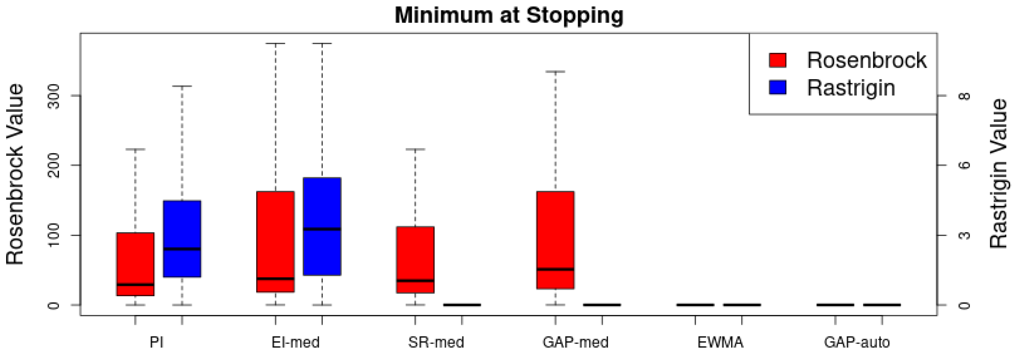
For the purpose of exploring the behavior of w in examples presented here, we use the following procedure for educating the choice of w. We hand tune w for two informative known example functions (i.e., Rosenbrock and Rastrigin). From the exploration of w in known examples, it is clear that w needs to increase directly with ELAI variance. Furthermore, if one considers the form of sample size calculations based on classical power analysis, sample size increases directly proportional with the sample variance. Thus, we linearly extrapolate the choice of w for two higher dimensional problems from the behavior of w in the hand-tuned test function examples. The value of w linearly increases from a value of 30 (based on sampling conventions) with a slope term structured to adjust the window size to the observed ELAI variance ($\widehat{v}$) in the new problems based on the sensitivity of the w estimates with the observed variances in the hand-tuned examples so that $\widehat{w}={\displaystyle \frac{\Delta w}{\Delta \mathrm{V}\left(\mathrm{ELAI}\right)}}\widehat{v}+30$.

3.5. Identifying Convergence

In identifying convergence, we not only hope that the ELAI series reaches a state of control, but we anticipate that the ELAI series demonstrates a move from pre-convergence to a consistent state of convergence. To recognize the move into convergence we combine the notion of the control window with the EWMA framework to construct the so called EWMA Convergence Chart. Since we expect EI values to decrease upon convergence, the primary recognition of convergence is that new ELAI values demonstrate values that are consistently lower than initial pre-converged values.

First, we require that all exponentially weighted $Z_s$ values inside the control window fall within the control limits. This ensures that the most recent ELAI values demonstrate distributional consistency within the bounds of the control window. Second, since we are looking for the point when the process changes from the initial pre-converged state of the system to a state of convergence, we require at least one point beyond the initial control window to fall outside the defined EWMA control limits. This second rule suggests that the new ELAI observations have established a state of control which is significantly different from the previous pre-converged ELAI observations. Jointly enforcing these two rules implies convergence based on the notion that convergence enjoys a state of consistently decreased expectation of finding new minima in future function evaluations.

Considering the optimization procedure outlined in Figure 2, the check for convergence indicated in step (7) amounts to computing new EWMA $Z_s$ values, and control limits, from the inclusion of the most recent observation of the improvement distribution, and checking if the subsequent set of $Z_s$ satisfy both of the above rules of the EWMA convergence chart. Satisfying one, or neither, of the convergence rules indicates insufficient exploration and further iterations of optimization are required to gather more information about the objective function. The time complexity of computing the EWMA convergence chart is $\mathcal{O}\left(T\right)$, which is fast relative to inference for the Gaussian process surrogate model.

4. Examples

We first look at two synthetic examples from the optimization literature, where the true optimum is known, so we can be sure we have converged to the true global minimum. We tune the EWMA Convergence Charts for each of these synthetic examples, then extrapolate the choices of w to provide a higher dimension test function and a real world example from hydrology.

4.1. Rosenbrock

The Rosenbrock function [21], $f(x_1,x_2)=100{\left(x_2-x_1^2\right)}^2+{(1-x_1)}^2$, was an early test problem in the optimization literature. It combines a narrow, flat parabolic valley with steep walls, and thus it can be difficult for gradient-based methods. Convergence is non-trivial to assess, because optimization routines can take some time to explore the relatively flat, but non-convex, valley floor for the global minimum. Here we focus on the region $-2\le x_1\le 2$, $-3\le x_2\le 5$. While the region around the mode presents some minor challenges, this problem is unimodal, and thus represents a relatively easier optimization problem in the context of Bayesian optimization, with a well-behaved convergence process.

We estimate $\lambda$ via the minimum $S_{\lambda }$ estimator, $\widehat{\lambda }\approx 0.5$. Due to the relative simplicity of this problem we find that $w=30$ results in a well-behaved convergence pattern with a final ELAI variance of $0.35$. Figure 4 shows the result of surrogate model optimization at convergence, as assessed by our method. The right panel shows the best function value (y-axis) found so far at each iteration (x-axis) and verifies that we have found the global minimum. The left panel shows the convergence chart, with the control window to the right of the vertical line, and the control limits indicated by the dashed lines. Iteration 74 is the first time that all EWMA points in the control window are observed within the control limits, and thus we declare convergence. This declaration of convergence comes after the global minimum has been found, but not too many iterations later, just enough to establish convergence. Note that the EWMA points generally trend downward until the global minimum is found at iteration 63.

4.2. Rastrigin

The 2-d Rastrigin function is a commonly used test function for evaluating the performance of global optimization schemes such as genetic algorithms [22], $f(x_1,x_2)={\sum }_{i=1}^2\left[x_i^2-10cos\left(2\pi x_i\right)\right]+2\left(10\right)$. The global behavior of Rastrigin is dominated by the spherical function, ${\sum }_i{x}_i^2$; however, Rastrigin has been oscillated by the cosine function and vertically shifted so that it achieves a global minimum value of 0 at the lowest point of its lowest trough at (0, 0). We search on the domain $-2.5\le x_i\le 2.5$. This function is highly multimodal, and the many similar modes present a challenge for identifying convergence. The multimodality of this problem increases the variability of the EI criterion and thus represents a moderately difficult optimization problem.

We estimate $\widehat{\lambda }\approx 0.4$. The decreased value of $\widehat{\lambda }$, relative to Rosenbrock, increases the smoothing capabilities of the EWMA procedure, as a response to the increased noise in the ELAI series. A larger w is needed to recognize convergence in the presence of increased noise in the ELAI criterion; $w=60$ was found to work well, with a final ELAI variance of $1.71$.

Figure 5 shows the convergence chart (left) and the optimization progress of the algorithm (right) after 115 iterations of optimization. Although the variability of the ELAI criterion increases as optimization proceeds, large ELAI values stop arriving after iteration 55, coincidentally with the surrogate model’s discovery of the Rastrigin’s main mode, as seen in the right panel of Figure 5. Furthermore, notice that optimization progress in Figure 5 (right) demonstrates that convergence in this case does indeed represent approximate identification of the theoretical minimum of the function, as indicated by the dashed horizontal line at the theoretical minimum.

4.3. Styblinski–Tang

The Styblinski–Tang function provides an example of a higher dimensional test function [23].

$$f\left(\mathit{x}\right)={\displaystyle \frac{1}{2}}\sum _{i=1}^d(x_i^4-16x_i^2+5x_i)x_i\in [-5,5]\forall i\in \{1,2,3,...d\},$$

(7)

where d is the dimension of the function. The function has a number of local models that flank the global mode and optimization of the function increases in difficulty in higher dimensions as the search space gains an increasing number of local modes with increasing d. Here we provide an example of a six-dimensional optimization of the Styblinski–Tang function with convergence monitored with the EWMA convergence chart.

In this example $\lambda$ is again estimated by minimizing the sum of squared forecasting deviations to be $\widehat{\lambda }\approx 0.4$. Using the automated method for determining the size of the control window based on the observed ELAI variance (0.92 here), a w of $50\approx \left({\displaystyle \frac{60-30}{1.71-0.35}}\right)0.92+30$ was used in this example.

Figure 6 shows the converged state of the Bayesian optimization procedure when first claiming convergence at iteration 134. The left panel of the figure demonstrates that convergence is identified by the chart when the final ELAI spike exits the control window and the ELAI series settles down as the surrogate model has found the global optimum (as seen in the right panel of the figure).

4.4. Lockwood Case Study

The previous examples have focused on analytical functions with known minima, helping develop an intuition for tuning the EWMA convergence chart parameters and to ensure that our methods correspond to the identification of real optima. Here we apply the EWMA convergence chart on the Lockwood pump and treat problem, originally presented by [24]. This case study considers an industrial site along the Yellowstone River in Montana, with groundwater contaminated by chlorinated solvents. Six pumps extract contaminated groundwater to attempt to prevent contamination of the river. The objective is to minimize the cost of running the pumps while preventing contamination of the river, and a computer simulator is used to compute the objective function.

The objective function, $f\left(\mathit{x}\right)$, to be minimized in this case, can be expressed as the sum of the pumping rates for each pump (a quantity proportional to the expense of running the pumps in US dollars), with additional large penalties associated with any contamination of the river.

$$f\left(\mathit{x}\right)=\sum _{i=1}^6{x}_i+2\left[c_a\left(\mathit{x}\right)+c_b\left(\mathit{x}\right)\right]+20,000\left[{\mathbb{1}}_{c_a\left(\mathit{x}\right)>0}+{\mathbb{1}}_{c_b\left(\mathit{x}\right)>0}\right]$$

(8)

Here, $c_a\left(\mathit{x}\right)$ and $c_b\left(\mathit{x}\right)$ are outputs of a simulation, indicating the amount of contamination, if any, of the river as a function of the pumping rates, $\mathit{x}$, for each of the six wells. Any amount of contamination of the river results in a large stepwise penalty which introduces a discontinuity into the objective function at the contamination boundary. Each $x_i$ is bounded on the interval $0\le x_i\le$ 20,000, representing a large range of possible management schemes. The full problem defines a six-dimensional optimization problem to determine the optimal rate at which to pump each well, so as to minimize the loss function defined in Equation (8). Since the loss function is defined over a large and continuous domain, and running the numerical simulation of the system is computationally expensive, this example presents an ideal situation for use with surrogate model-based optimization.

By using the fitted values of w and the observed ELAI variance in each of the two previous examples, we extrapolate an appropriate value of w for this case study based on an observed ELAI variance of $2.86$, resulting in an estimated w of $93\approx \left({\displaystyle \frac{60-30}{1.71-0.35}}\right)2.86+30$, as discussed in Section 3.4. $\lambda$ was chosen via the minimum $S_{\lambda }$ estimator to be $\widehat{\lambda }\approx 0.4$. This level of smoothing is required here to reduce the noise in the ELAI criterion due to the large search domain, as well as the complicated contamination boundary among the six wells. Furthermore, these features of the objective function complicate fit of the surrogate model and thus more function evaluations are required to produce an accurate model of f.

The convergence chart for monitoring the optimization of the Lockwood case study is shown in the left panel of Figure 7. Convergence in this case does not occur with a dramatic shift in the mean level of the ELAI criterion, but rather convergence occurs as the series stabilizes after large ELAI values move beyond the control limit. Interestingly, the last major spike in the ELAI series is observed alongside the discovery of the final major jump in the current best minimum value as seen at about iteration 180 in the right panel of Figure 7. The EWMA convergence chart identifies convergence as the EWMA statistic associated with this final ELAI spike eventually exits the control window at iteration 270. The solution shown here corresponds to $f\left(\mathit{x}\right)\approx \mathrm{26,696}$. This solution is corroborated as a point of diminishing returns by the analysis of [25] on the same problem, as seen in their average EI surrogate modeling behavior.

5. Experimental Comparison

The EWMA convergence chart is benchmarked against other Bayesian optimization stopping criteria by using a modified version of the code provided by [6], where they propose regret-based stopping criteria (https://github.com/hideaki-ishibashi/stopping_BO, accessed on 17 September 2025). The EWMA convergence charting method presented here is compared against 0.01 times the median of Expected Improvement (EI-med), simple regret (SR-med), and the gap of expected minimum simple regrets (GAP-med), as well as thresholds derived from probability of improvement (PI) and the adaptive method based on the gap of expected minimum simple regrets (GAP-auto), each of which is detailed in [6]. The experiment is run on the Rosenbrock and Rastrigin test functions as specified in Section 4.1 and Section 4.2 above, each with global minimum values of zero.

Fifty test optimizations of each function are performed while evaluating each stopping criterion. The stopping time declared by each method, along with the minimum objective value at stopping, are recorded to evaluate if each stopping method finds the global minimum correctly, while also stopping as early as possible. The false positive rate (F.P.R.) of each method is calculated by enumerating the number of runs that discover minimum objective values within $0.01$ of the global minimum at stopping.

Figure 8 summarizes each of the objective function minimum values at stopping for each stopping criterion as boxplots over the fifty simulation runs. The PI and EI-med stopping criteria struggle to regularly find the global minimum for both functions. The SR-med and GAP-med criteria both struggle with Rosenbrock, but regularly converge to the global minimum on Rastrigin. The EWMA convergence chart and the GAP-auto method are the only methods tested that regularly find the global minimum of both test functions.

Table 1. Stopping false positive rate (F.P.R.) based on a $0.01$ region about the global minimum and average stopping time (S.T.) of each stopping criterion.

Stopping Criteria	Rosenbrock		Rastrigin
	F.P.R.	S.T.	F.P.R.	S.T.
PI	0.93	34	0.88	60
EI-med	1.00	26	0.86	59
SR-med	1.00	31	0.04	205
GAP-med	1.00	26	0.04	204
EWMA	0.11	256	0.02	248
GAP-auto	0.02	269	0.00	411

demonstrates how well each function achieves the goal of finding the global minimum while stopping as early as possible. Methods that show a low F.P.R., while having the lowest possible stopping time (S.T.) achieve both goals well. As previously established, the EWMA convergence chart and GAP-auto criteria are the only methods tested that regularly find the global minimum for both functions. However, for the Rastrigin test function, the GAP-auto criterion appears to be overly risk averse, achieving the global optimum in every single simulation but requiring far more function evaluations than EWMA. The EWMA has a similarly low F.P.R. (only allowing a single false positive), but stops much earlier on average, requiring about 60% of the function evaluations as the GAP-auto method. We also note that the GAP methods are tuned for GP surrogates and are not as easily extensible to other surrogate models.

Table 2. Average run time (ms) of each stopping criterion as run on Rosenbrock.

Stopping Criteria	Run Time
PI	15
EI-med	11
SR-med	18
GAP-med	24
EWMA	39
GAP-auto	36

shows the average wall clock run time of 500 timings of each criterion timed on an AMD Ryzen 7 7840U CPU. The EWMA criterion run time is comparable to the other GAP methods in this setting. The EWMA criterion extends to other surrogate models with similar run times, while the GAP methods rely on a GP surrogate to achieve these run times. That said, each stopping criterion runs in tens of milliseconds within a GP model that runs in hundreds or thousands of milliseconds. Updating the GP model and predicting the next acquisition location runs in an average of 620 ms on the same example timings without the convergence criteria calculations. This demonstrates the relatively minor computational cost of the stopping criteria.

6. Conclusions

Adapting the notion of control from the SPC literature, the EWMA convergence chart outlined here aims to provide an objective standard for identifying convergence in the presence of the inherent stochasticity of the improvement criterion in this setting. The examples provided here demonstrate how the EWMA convergence chart may accurately and efficiently identify convergence in the context of Bayesian optimization. We note that our approach could be applied with any optimization algorithm that allows computation of an expected improvement at each iteration.

As for any optimization algorithm, a converged solution may only be considered as good as the algorithm’s exploration of f. Thus, poorly tuned strategies may never optimize f to their fullest extent, but the EWMA convergence chart presented here may still claim convergence in these cases. The EWMA convergence chart may only consider convergence in the context of the algorithm in which it is embedded and should be interpreted as a means of identifying when a global algorithm has converged. At which point, it is beneficial to stop iterating the routine and reflect upon the results. Finally, it is worth noting that in any stochastic environment, there is no guarantee of accurate prediction of convergence. We have found that our approach works well in a variety of settings, but it is possible for it to prematurely declare convergence. That said, this balanced tolerance to risk allows the EWMA chart to effectively weight the sensitivity to declare convergence against the desire to stop as early as possible.