Article

A Note on Rational Lagrange Polynomials for CAGD Applications and Isogeometric Analysis

by
Christopher Provatidis
School of Mechanical Engineering, National Technical University of Athens, 9 Iroon Polytechniou Str., 15780 Athens, Greece
Mathematics 2025, 13(20), 3239; https://doi.org/10.3390/math13203239
Submission received: 11 September 2025 / Revised: 1 October 2025 / Accepted: 5 October 2025 / Published: 10 October 2025

Abstract

While the established theory of computer-aided geometric design (CAGD) suggests that rational Bernstein–Bézier polynomials associated with control points can be used to accurately represent conics and quadrics, this paper shows that the same goal can be achieved in a different manner. More specifically, rational Lagrange polynomials of the same degree, associated with nodal points lying on the true curve or surface, can be combined with appropriate weights to yield equivalent numerical results within a Bézier patch. The specific application of this equivalence to derive weights for Lagrange nodes on conics and quadrics is shown in this paper. Although this replacement may not be crucial for CAGD purposes, it proves useful for the direct implementation of boundary conditions in isogeometric analysis, since it allows the use of nodal values on the exact boundary.

1. Introduction

Since the mid-1970s, research in computer-aided geometric design (CAGD) has heavily relied on Bernstein–Bézier polynomials as a foundational tool for representing and manipulating curves and surfaces. This preference stems primarily from their strong geometric intuition: the shape of a Bézier curve or surface is governed by a finite set of control points, which usually lie outside the geometric entity itself and act as handles for interactive design and editing. A second important reason is the mathematical flexibility of the Bernstein basis, which supports essential operations such as degree elevation, subdivision, and knot insertion, enabling local refinement without altering the global geometry’s key features for adaptive modeling and analysis [1].
Furthermore, Bernstein polynomials are central to the construction of non-uniform rational B-splines (NURBSs), which extend polynomial representations by incorporating weights. This allows for the exact representation of conic sections and other analytic shapes, a capability critical to engineering design and manufacturing applications. As a result, Bernstein-based representations remain a cornerstone of modern computer-aided design and computer-aided manufacturing (CAD/CAM) systems and form the basis of isogeometric analysis, which unifies geometric modeling [1,2,3], finite element analysis [4], and boundary element analysis [5].
It is well established in the literature that the weighted, or rational, Bernstein–Bézier formulation enables the exact representation of conic sections and quadrics, provided that suitable weights are assigned to the appropriate control points (e.g., see [1,2,3], among hundreds of other sources). This capability is one of the key advantages of rational Bézier and NURBS representations in computer-aided geometric design and CAD systems. However, there have also been a limited number of investigations into using Lagrange polynomials for similar geometric modeling tasks, particularly for approximating circular arcs and ellipses, but for efficient isogeometric analysis as well [6,7]. Focusing on circular arcs, these approaches can produce visually acceptable results but typically suffer from small but non-negligible numerical errors due to the inability of polynomial Lagrange interpolation to exactly represent circular shapes [8,9,10,11].
On the other hand, Lagrange interpolation in itself is quite robust and efficient. The mentioned instabilities are related to Runge oscillations, which only occur on equidistant nodal distributions (for example, see Ref. [12]). Within this context, Lagrange interpolation might break down in such a case for high polynomial orders. However, a simple remedy is to use non-equidistant nodal distributions that accumulate nodes near the interval boundaries. This has been done in the Spectral Element Method (SEM), where Gauss–Lobatto–Legendre (GLL) or Gauss–Lobatto–Chebyshev (GLC) nodes are employed to replace equidistant nodes [13,14]. Such non-equidistant nodes result in excellent interpolation properties and mitigate any instabilities. Employing GLL or GLC nodes, it has been noticed that the element matrices are well conditioned, and numerical problems do not arise [15].
From the above discussion, it follows that Lagrange polynomials offer high accuracy when applied in conjunction with non-equidistant nodal distributions (e.g., GLL or GLC points), whereas Bernstein polynomials possess the advantage of incorporating weights that enable the exact representation of conics and quadrics.
In this paper, we lay the groundwork for combining these two advantages into a unified framework. Specifically, we determine the nodal coordinates and the associated weights that can be directly applied to both uniform and non-uniform Lagrange polynomials, thereby establishing an equivalent functional basis of rational Lagrange polynomials within a rational Bézier curve or a rational Bézier patch.
The present paper is structured as follows: Section 2 introduces the transformation matrix from Bernstein to Lagrange polynomials. Section 3 derives the weights applicable to Lagrange polynomials when nodal points lie on the true curve. Section 4 presents illustrative examples of a circular arc. Section 5 extends the proposed method to a spherical cap. Section 6 addresses the numerical implementation for tensor-product surfaces of arbitrary topology. Section 7 reports numerical solutions of a two-dimensional boundary-value problem governed by the Laplace equation. Section 8 provides a discussion that places the findings in context and highlights their implications. Finally, Section 9 summarizes the main conclusions and outlines directions for future work.

2. General Formulation

2.1. Degree Elevation Using Bernstein–Bézier Polynomials

Rational Bézier curves can be readily handled within the framework of computer-aided geometric design (CAGD). Beginning with a low degree, such as n = 2 , and employing an appropriate set of homogeneous (projected) control points P 0 w , , P n w , with weights ( w i , i = 0 , , n ), the shape of the curve remains invariant under degree elevation, with the control points being updated accordingly at each step as follows:
Q i w = ( 1 a i ) P i w + a i P i 1 w ,
with
a i = i n + 1 , i = 1 , , n .
The updated homogeneous weights w i * that accompany the elevated control points Q i w = w i * [ x i * , y i * , z i * ] T (or the 2-D analogue) follow exactly the same convex-combination pattern as for the degree elevation formula for Bernstein (polynomial) Bézier curves (cf. Equation (1)):
w i * = i n + 1 w i 1 + 1 i n + 1 w i , i = 1 , , n ,
with the boundary values preserved,
w 0 * = w 0 , w n + 1 * = w n .
Once the homogeneous points are updated, we obtain the control points (in Cartesian coordinates) simply by dehomogenising:
Q i = Q i w w i * , i = 0 , , n + 1 .
This degree-elevation step may be applied repeatedly; after k successive elevations (to degree n + k ), the same recurrence is used at each stage, guaranteeing that the rational Bézier curve’s shape remains unchanged, while its control-polygon flexibility increases.

2.2. Replacing Bernstein Polynomials with Lagrange Polynomials

While the procedure of degree elevation is straightforward in conjunction with Bernstein polynomials, this is not the case with Lagrange polynomials. Of course, since both sets span the same space (of powers ξ i , i = 0 , ), these two sets are linearly interrelated.
In more detail, let us consider the reference unit length 0 ξ 1 . For a certain degree n, i.e., for the nodal points 0 = ξ 0 , , ξ n = 1 , let L be the column vector (of size ( n + 1 ) × 1 ) including all relevant univariate Lagrange polynomials of degree n (the superscript stands for the transpose):
L = [ L 0 ( ξ ) , , L n ( ξ ) ] ,
and B be the column vector (of size ( n + 1 ) × 1 ) including all univariate Bernstein polynomials of degree n:
B = [ B 0 ( ξ ) , , B n ( ξ ) ] .
Then, we can write
L = T B L B ,
and
B = T L B L ,
where T B L (from Bernstein to Lagrange) and T L B (from Lagrange to Bernstein) are transformation matrices, which have been discussed in detail elsewhere [16]. For the purposes of this paper, the determination of transformation matrix T L B that must be applied to Lagrange polynomials—according to Equation (9)—plays a critical role. This issue is discussed in detail in Section 2.5.
Actually, since a linear transformation occurs between two functional sets (here, the subscripts are B: Bernstein–Bézier; L: Lagrange), not only the different sets of polynomials (cf. Equations (8) and (9)) but also the homogeneous coordinates ( Q L w , P B w ) and the weights ( w L , w B ) are interrelated according to the theorem detailed below. Note that each of the matrices ( Q L w , P B w ) is an array of size ( n + 1 ) × 3 , where the first column corresponds to the x-coordinates, the second to the y-coordinates, and the third to the z-coordinates of nodal points or control points. Moreover, each of ( w L , w B ) is a column vector of size ( n + 1 ) × 1 .
Theorem 1.
The homogeneous (projected) cordinates of nodal points ( Q L w ) associated with the true boundary of curve C ( ξ ) in the Lagrange formulation are related to the projected control points ( P B w ) of the same curve in the Bernstein formulation, as follows:
Q L w = T L B P B w .
Moreover, weights w L in the Lagrange formulation are related to weights w B in the initial Bernstein formulation, as follows:
w L = T L B w B .
In more detail, to obtain the nodal points Q L on the true curve, it is necessary to divide the vector of homogeneous coordinates Q L w (calculated using Equation (10)) by the vector of associated weights w L (estimated by Equation (11)).
Proof. 
The proof is based on the fact that the shape x ( ξ ) = [ x ( ξ ) , y ( ξ ) , z ( ξ ) ] of the curve under consideration is preserved (in shape and parametrically [2]). Therefore, expressing x ( ξ ) first in terms of Lagrange polynomials (forming the vector L ) and second in terms of Bernstein polynomials (forming the vector B ), we have
x ( ξ ) = L Q L w L w L = B P B w B w B .
Substituting B through Equation (9) into the utmost right term of Equation (12), we obtain
x ( ξ ) = L Q L w L w L = ( T L B L ) P B w ( T L B L ) w B = L ( T L B P B w ) L ( T L B w B ) .
Obviously, the last equality of Equation (13) suggests that Equations (10) and (11) provide the projected nodal points and associated weights, respectively, and this completes the proof.    □
Remark 1.
Weights. In a previous work (see pp. 80–83, [16]) regarding a circular arc of 90 degrees modeled by quadratic Bernstein polynomials, Equation (11) was proven from scratch (after manipulation), but here the formula was generalized in matrix form for any degree n.
Therefore, if we restrict our study, for example, to a circular arc with a central angle of 90°, we may begin with a quadratic polynomial ( n = 2 ) associated with the weights w = [ 0 , 2 2 , 1 ] (see, Ref. [17]). Subsequently, Equation (3) can be applied to compute the weights resulting from successive degree elevations until a certain degree n > 2 .
For each of the abovementioned degree elevations, we can determine the transformation matrix T L B , and then implement Equation (11) to determine the weights associated with the rational Lagrange polynomials.
Remark 2.
Nodal points. By definition, non-uniform rational B-splines (NURBS) are a non-uniform interpolation. This means that even if the interval [ 0 , 1 ] is uniformly subdivided by the points ξ = [ 0 , 1 n , , ( n 1 ) n , 1 ] , the corresponding nodal points do not generally subdivide the curve C ( ξ ) in equal arc lengths. This issue is shown later in Section 3.1.2.

2.3. Determination of Transformation Matrix

In this section, we present two alternative procedures for constructing the transformation matrix.

2.3.1. Detailed Algebraic Procedure

Since Bernstein and Lagrange polynomials span the same space (of monomials ξ i , i = 0 , 1 , , n ), any univariate function U ( ξ ) will be equally written in any of them. By equating the coefficients of the same powers ξ i , we can derive a relationship between nodal values U i and generalized coefficients a i . This relationship is set in the form
U nodal = T L B a .
Example 1.
Let us set function U ( ξ ) in terms of quadratic Lagrange polynomials (based on uniform nodal points at ξ = 0 , 1 2 , 1 ), as follows:
U ( ξ ) = L 0 , 2 ( ξ ) U 0 + L 1 , 2 ( ξ ) U 1 + L 2 , 2 ( ξ ) U 2 = ( 2 ξ 2 3 ξ + 1 ) U 0 + ( 4 ξ 2 + 4 ξ ) U 1 + ( 2 ξ 2 ξ ) U 2 = ξ 2 ( 2 U 0 4 U 1 + 2 U 2 ) + ξ ( 3 U 0 + 4 U 1 U 2 ) + U 0 .
Alternatively, let us set the same function U ( ξ ) in terms of Bernstein polynomials:
U ( ξ ) = B 0 , 2 ( ξ ) a 0 + B 1 , 2 ( ξ ) a 1 + B 2 , 2 ( ξ ) a 2 = ( 1 ξ ) 2 a 0 + 2 ( 1 ξ ) ξ a 1 + ( ξ 2 ) a 2 = ( ξ 2 2 ξ + 1 ) a 0 + ( 2 ξ 2 + 2 ξ ) a 1 + ( ξ 2 ) a 2 = ξ 2 ( a 0 2 a 1 + a 2 ) + ξ ( 2 a 0 + 2 a 1 ) + a 0 .
By equating the coefficients of the same powers between the quadratic polynomials given by Equations (15) and (16), we obtain the following system:
2 U 0 4 U 1 + 2 U 2 = a 0 2 a 1 + a 2 3 U 0 + 4 U 1 U 2 = 2 a 0 + 2 a 1 U 0 = a 0 .
Equivalently, Equation (17) can be written as follows:
2 4 2 3 4 1 1 0 0 U 0 U 1 U 2 = 1 2 1 2 2 0 1 0 0 a 0 a 1 a 2 .
Equation (18) can be solved for either of the two vectors. Choosing the second one, after matrix inversion, we have
a 0 a 1 a 2 = 1 0 0 1 2 2 1 2 0 0 1 U 0 U 1 U 2 .
Inserting the three coefficients from Equation (19) into Equation (16), we have
U ( ξ ) = B 0 , 2 ( ξ ) a 0 + B 1 , 2 ( ξ ) a 1 + B 2 , 2 ( ξ ) a 2 = B 0 , 2 ( ξ ) U 0 + B 1 , 2 ( ξ ) ( 1 2 U 0 + 2 U 1 1 2 U 2 ) + B 2 , 2 ( ξ ) U 2 = B 0 , 2 ( ξ ) 1 2 B 1 , 2 ( ξ ) U 0 + 2 B 1 , 2 ( ξ ) U 1 + 1 2 B 1 , 2 ( ξ ) + B 2 , 2 ( ξ ) U 2 .
Comparing Equation (20) with the first equality of Equation (15), the unique representation—in terms of ( U 0 , U 1 , U 2 )—leads to the following relationships:
L 0 , 2 ( ξ ) = B 0 , 2 ( ξ ) 1 2 B 1 , 2 ( ξ ) , L 1 , 2 ( ξ ) = 2 B 1 , 2 ( ξ ) , L 2 , 2 ( ξ ) = 1 2 B 1 , 2 ( ξ ) + B 2 , 2 ( ξ ) .
In matrix form, Equation (21) is rewritten as
L 0 , 2 ( ξ ) L 1 , 2 ( ξ ) L 2 , 2 ( ξ ) = 1 1 2 0 0 2 0 0 1 2 1 T B L B 0 , 2 ( ξ ) B 1 , 2 ( ξ ) B 2 , 2 ( ξ ) .
By inverting Equation (22), we receive
B 0 , 2 ( ξ ) B 1 , 2 ( ξ ) B 2 , 2 ( ξ ) = 1 1 4 0 0 1 2 0 0 1 4 1 T L B L 0 , 2 ( ξ ) L 1 , 2 ( ξ ) L 2 , 2 ( ξ ) .
Therefore, if we pack all triplets into the relevant column vectors
U = U 0 U 1 U 2 , a = a 0 a 1 a 2 , L = L 0 , 2 ( ξ ) L 1 , 2 ( ξ ) L 2 , 2 ( ξ ) , B = B 0 , 2 ( ξ ) B 1 , 2 ( ξ ) B 2 , 2 ( ξ ) ,
the above relationships are written in matrix form as follows:
L = T B L B , B = T L B L ,
and
a = T B L U , U = T L B a ,
with
T B L = ( T L B ) 1 .

2.3.2. A Shorter Numerical Procedure

Since the transformation matrices simply relate the nodal vector U to the coefficient vector a as given in Equation (26), in a unique manner (due to the same polynomial degree), we can begin by implementing the well-known formula
U ( ξ ) = i = 0 2 B i , 2 ( ξ ) a i ,
at the uniform points ξ = 0 , 1 2 , 1 (with which the nodal values U 0 , U 1 , U 2 are associated), and thus we shortly obtain
U 0 U 1 U 2 = B 0 , 2 ( 0 ) B 1 , 2 ( 0 ) B 2 , 2 ( 0 ) B 0 , 2 ( 1 2 ) B 1 , 2 ( 1 2 ) B 2 , 2 ( 1 2 ) B 0 , 2 ( 1 ) B 1 , 2 ( 1 ) B 2 , 2 ( 1 ) a 0 a 1 a 2 = 1 0 0 1 4 1 2 1 4 0 0 1 T L B a 0 a 1 a 2 .
Therefore, by applying the Bernstein-based series expansion Equation (28) at three points on the true curve associated with uniform parameters ξ , we can shortly obtain the transpose of the transformation matrix T L B :
T L B = B 0 , 2 ( 0 ) B 1 , 2 ( 0 ) B 2 , 2 ( 0 ) B 0 , 2 ( 1 2 ) B 1 , 2 ( 1 2 ) B 2 , 2 ( 1 2 ) B 0 , 2 ( 1 ) B 1 , 2 ( 1 ) B 2 , 2 ( 1 ) = 1 0 0 1 4 1 2 1 4 0 0 1
which denotes the change from the Lagrange (L) to the Bernstein (B) basis.
The generalization of the above procedure to an arbitrary degree p is presented in Section 2.5.

2.4. From Approximation Theory and Numerical Analysis to CAGD

In this subsection, we continue the discussion, restricting it to p = 2 .
The conclusions of Section 2.3 pertain to the relationship between the nodal values U i and the generalized coefficients a i . Within the context of computer-aided geometric design (CAGD), the nodal values U i correspond to the Cartesian coordinates of nodal points Q L i = [ x i c , y i c , z i c ] (i.e., of size 1 × 3 ) on the true curve C ( ξ ) , whereas the generalized coefficients a i are interpreted as control points P i = [ x i c , y i c , z i c ] (each of them is of size 1 × 3 ), which form an exoskeleton of curve C ( ξ ) .
Within this context, in non-rational formulation, the substitute of Equation (28) is
x ( ξ ) = i = 0 2 B i , 2 ( ξ ) P i ,
where x ( ξ ) = [ x ( ξ ) , y ( ξ ) , z ( ξ ) ] (i.e., of size 1 × 3 ).
Therefore, when the weights are equal to unity ( w B i = 1 ), Equation (31) can be applied at nodal points Q L i = [ x i c , y i c , z i c ] on the exact curve (at specific—thus far uniform—parameter values ξ ) and then solved for P i . Next, we show that the matrix relating the three nodal points Q L (of size 3 × 3 ) and the three control points P (of size 3 × 3 ) is
Q L = T L B P ,
where T L B is the aforementioned transformation matrix of size 3 × 3 , defined in Equation (30).
Actually, when the weights are non-unit ( w B i 1 ), Equation (31) extends to
x ( ξ ) = i = 0 2 B i , 2 ( ξ ) P i w i = 0 2 B i , 2 ( ξ ) w B i = B 0 , 2 ( ξ ) , B 1 , 2 ( ξ ) , B 2 , 2 ( ξ ) P 0 w P 1 w P 2 w i = 0 2 B i , 2 ( ξ ) w B i = B 0 , 2 ( ξ ) , B 1 , 2 ( ξ ) , B 2 , 2 ( ξ ) P w B 0 , 2 ( ξ ) , B 1 , 2 ( ξ ) , B 2 , 2 ( ξ ) w B ,
where the projected (homogeneous) control points, packed into matrix P w of size 3 × 3 , are given by the well-known formula
P w = P 0 w P 1 w P 2 w w B 0 P 0 w B 1 P 1 w B 2 P 2 .
Depending on the value of parameter ξ = { 0 , 1 2 , 1 } , the row vector [ B 0 , 2 ( ξ ) , B 1 , 2 ( ξ ) , B 2 , 2 ( ξ ) ] (of size 1 × 3 ) in the numerator of Equation (33) is one out of the three rows of matrix T L B T involved in Equation (30). In more detail, considering Equation (34), we have
Q L 0 = B 0 , 2 ( 0 ) B 1 , 2 ( 0 ) B 2 , 2 ( 0 ) P w B 0 , 2 ( 0 ) , B 1 , 2 ( 0 ) , B 2 , 2 ( 0 ) w B
Q L 1 = B 0 , 2 ( 1 2 ) B 1 , 2 ( 1 2 ) B 2 , 2 ( 1 2 ) P w B 0 , 2 ( 1 2 ) , B 1 , 2 ( 1 2 ) , B 2 , 2 ( 1 2 ) w B
Q L 2 = B 0 , 2 ( 1 ) B 1 , 2 ( 1 ) B 2 , 2 ( 1 ) P w B 0 , 2 ( 1 ) , B 1 , 2 ( 1 ) , B 2 , 2 ( 1 ) w B .
The totality of Equations (35)–(37) forms matrix Q L of nodal points on curve C ( ξ ) (for p = 2 , this matrix is of size 3 × 3 ), which was calculated at the uniform values of parameter ξ :
Q L = Q L 0 Q L 1 Q L 2 .
From Equations (35)–(37) it is also concluded that, in terms of the projected control points P w , we can calculate the projected nodal coordinates (generally located outside the true curve C ( ξ ) ), as follows (see also Equation (10)):
Q L w = T L B P w ,
where
Q L w = w L 0 Q L 0 w L 1 Q L 1 w L 2 Q L 2 ,
with (see also Equation (11))
w L = w L 0 w L 1 w L 2 .
Based on the three nodal points Q L given by Equation (40), we shall now show how they can be incorporated into the formulation of the geometry description.
The first step is to rewrite the denominator of Equation (33), so that its last equality becomes
x ( ξ ) = B 0 , 2 ( ξ ) , B 1 , 2 ( ξ ) , B 2 , 2 ( ξ ) P w B 0 , 2 ( ξ ) , B 1 , 2 ( ξ ) , B 2 , 2 ( ξ ) w B ,
where w B is the column vector of the abovementioned weights in the classical Bernstein formulation:
w B = w B 0 w B 1 w B 2 .
The second step is to substitute the row vector B = B 0 , 2 ( ξ ) , B 1 , 2 ( ξ ) , B 2 , 2 ( ξ ) of Bernstein polynomials (of size 1 × 3 ) in both the numerator and denominator of Equation (33), by row vector L (using the second equality of Equation (25)), as follows:
x ( ξ ) = L 0 , 2 ( ξ ) L 1 , 2 ( ξ ) L 2 , 2 ( ξ ) T L B P w L 0 , 2 ( ξ ) L 1 , 2 ( ξ ) L 2 , 2 ( ξ ) T L B w B .
The third step is to apply Equations (10) and (11) to the numerator and denominator of Equation (44), respectively, and thus it eventually becomes
x ( ξ ) = L 0 , 2 ( ξ ) L 1 , 2 ( ξ ) L 2 , 2 ( ξ ) Q L w L 0 , 2 ( ξ ) L 1 , 2 ( ξ ) L 2 , 2 ( ξ ) w L .
Regarding Equation (45), one may observe that in the numerator, weights w L i have been incorporated into the projected (homogeneous) nodal coordinates Q L i w w L i Q L i , which are related to—but generally do not coincide with—the i-th projected control point P i w w i P i ( i = 0 , 1 , 2 ). The denominator, on the other hand, consists of the product of the Lagrange polynomials associated with the three nodal points and the weight column vector w L in the Lagrangian system.
It is worth mentioning that although the three nodal points ( Q L 0 , Q L 1 , Q L 2 ) subdivide the circular arc into two equal parts, due to the presence of weights w L i , the mapping from the parameter space to the physical space is, in general, non-uniform, even if each part is further subdivided into uniform increments Δ ξ . This implies that increments Δ α of the corresponding central angles will also be non-uniform, as will be further discussed in Section 3.1.2.

2.5. General Procedure for the Determination of Transformation Matrix T L B

2.5.1. Uniform Points

For any arbitrary polynomial degree p, Equation (28) is generalized as follows:
U ( ξ ) = i = 0 p B i , p ( ξ ) a i .
Then, Equation (46) is applied to the set of uniform points ξ = 0 , 1 p , , p 1 p , 1 (with which the nodal values U 0 , U 1 , , U p 1 , U p are associated), and thus we eventually obtain
T L B T = B 0 , p ( 0 ) B 1 , p ( 0 ) B p 1 , p ( 0 ) B p , p ( 0 ) B 0 , p ( 1 p ) B 1 , p ( 1 p ) B p 1 , p ( 1 p ) B p , p ( 1 p ) B 0 , p ( p 1 p ) B 1 , p ( p 1 p ) B p 1 , p ( p 1 p ) B p , p ( p 1 p ) B 0 , p ( 1 ) B 1 , p ( 1 ) B p 1 , p ( 1 ) B p , p ( 1 ) ,
where the Bernstein polynomials of degree p are given by
B i , p ( ξ ) = p i ξ i ( 1 ξ ) p i , for i = 0 , 1 , , p .
Two methods are available for computing the Bernstein polynomials in Equation (47), as follows:
  • Direct evaluation via Equation (48);
  • Utilization of efficient B-spline algorithms using the knot vector
    Ξ = [ 0 , , 0 p + 1 , 1 , , 1 p + 1 ]
    (see, [12]), an example of which is the spcol function in MATLAB ver. R2025a.
Obviously, for a polynomial degree p, transformation matrix T L B is of size ( p + 1 ) × ( p + 1 ) .
A library of transformation matrices, T L B , for  p = 2 , , 6 , together with the corresponding weight vectors w L , is provided in Section 3.

2.5.2. Non-Uniform Points

A similar procedure is followed when points ξ to which Equation (46) is applied are non-uniform. Equation (47) holds again, but is applied to a set of points ξ i non-uniformly distributed in the interval [ 0 , 1 ] . An example is given in Section 3.1.2.

3. Weights

3.1. Circular Arc with Central Angle 90°

3.1.1. Uniform Distribution

We consider a circular arc of central angle 90° and radius R = 1 in the first quadrant. We start with degree p = 2 in conjunction with the well-known control points P 0 ( 1 , 0 ) , P 1 ( 1 , 1 ) , and  P 2 ( 0 , 1 ) , and the initial weights ( w 0 = 1 , w 1 = 2 2 , w 2 = 1 , according to [17]).
As a first step, we continuously elevate the polynomial degree applying Equation (3), thus determining the updated weights for each degree. Furthermore, applying Equation (1), we determine the Lagrange-based weights.
The second step is to determine the transpose of transformation matrix T L B for the desired degree p. Collectively, by implementing Equation (47) for degrees p = 2 until p = 6 , we obtain
( T L B ) p = 2 = 1 0 0 1 / 4 1 / 2 1 / 4 0 0 1
( T L B ) p = 3 = 1 0 0 0 8 / 27 4 / 9 2 / 9 1 / 27 1 / 27 2 / 9 4 / 9 8 / 27 0 0 0 1
( T L B ) p = 4 = 1 0 0 0 0 81 / 256 27 / 64 27 / 128 3 / 64 1 / 256 1 / 16 1 / 4 3 / 8 1 / 4 1 / 16 1 / 256 3 / 64 27 / 128 27 / 64 81 / 256 0 0 0 0 1
( T L B ) p = 5 = 1 0 0 0 0 0 541 / 1651 256 / 625 128 / 625 32 / 625 4 / 625 1 / 3125 243 / 3125 162 / 625 216 / 625 144 / 625 48 / 625 32 / 3125 32 / 3125 48 / 625 144 / 625 216 / 625 162 / 625 243 / 3125 1 / 3125 4 / 625 32 / 625 128 / 625 256 / 625 541 / 1651 0 0 0 0 0 1
( T L B ) p = 6 = 1 0 0 0 0 0 0 214 / 639 428 / 1065 214 / 1065 234 / 4367 125 / 15552 5 / 7776 1 / 46656 64 / 729 64 / 243 80 / 243 160 / 729 20 / 243 4 / 243 1 / 729 1 / 64 3 / 32 15 / 64 5 / 16 15 / 64 3 / 32 1 / 64 1 / 729 4 / 243 20 / 243 160 / 729 80 / 243 64 / 243 64 / 729 1 / 46656 5 / 7776 125 / 15552 234 / 4367 214 / 1065 428 / 1065 214 / 639 0 0 0 0 0 0 1 .
The associated weights, computed using Equation (11), are listed in Table 1.

3.1.2. Non-Uniform Distribution

Now, we consider the case of non-uniform distribution of nodal points along the edges of a 27-node classical transfinite element (shown in Figure 1), where the nodes along the horizontal edge AB are located at non-uniform positions:
ξ = 0 , 1 6 , 2 6 , 3 6 , 3 4 , 1 .
The formulation follows Equation (47), where the Bernstein polynomials are evaluated at the ξ -vector given in Equation (54). Consequently, the transformation matrix takes the following form:
( T L B ) p = 5 non uniform = 1 0 0 0 0 0 428 / 1065 428 / 1065 625 / 3888 125 / 3888 25 / 7776 1 / 7776 32 / 243 80 / 243 80 / 243 40 / 243 10 / 243 1 / 243 1 / 32 5 / 32 5 / 16 5 / 16 5 / 32 1 / 32 1 / 1024 15 / 1024 45 / 512 135 / 512 405 / 1024 243 / 1024 0 0 0 0 0 1 ,
whence the updated associated weight vector (according to Equation (11)) becomes
w L = 1 26 + 5 2 36 5 + 2 2 9 2 + 2 4 10 + 3 2 16 1 .
One may observe in Equation (56) that the non-uniform node distribution (Equation (54)) leads to the non-symmetric form of vector w L .
In the following section, we shall demonstrate that—using Equations (55) and (56)—both a straight segment and a circular arc can be represented accurately.
  • Straight segment
Taking the uniform set of control points associated with the Bernstein basis of degree p = 5 (in the x-direction, considering weights w B = 1 , whereas y = z = 0 ),
P B w = P B = 0 , 1 5 , 2 5 , 3 5 , 4 5 , 1 ,
and left-multiplying by the non-uniform transformation matrix given by in Equation (55) according to Equation (10), we derive the true non-uniform x-coordinates (obviously w L = 1 ):
Q nodal = ( T L B ) p = 5 non uniform · P B w = 0 , 1 6 , 2 6 , 3 6 , 3 4 , 1 .
The result of Equation (58) is validated by the non-uniform nodal points shown on edge AB of Figure 1.
Remark 3.
In contrast, if the uniform set of Equation (57) had been multiplied by the uniform matrix of Equation (52), the location of the nodal points on the straight segment would be uniform as well.
II.
Circular arc
The projected coordinates in the Lagrange formulation can be computed from Equation (10), using the Cartesian coordinates of the control points in the Bernstein formulation (Table 2) together with the associated weights in Table 1. Subsequently, these projected coordinates are divided by the corresponding entries of the column vector w L given in Equation (56), thereby yielding the Cartesian coordinates.
The results of the above procedure are illustrated in Figure 2, where the nodal sequence {1,2,3,4,5,6} of the Lagrangian formulation is oriented counterclockwise. The five central angles formed by the radii corresponding to the endpoints of each nodal segment (i.e., 1–2, …, 5–6) are listed in Table 2. It can be observed that nodal point 4 (at ξ = 0.50 ) lies exactly at the midpoint of the circular arc (i.e., a 1 + a 2 + a 3 = 45 ° ). However, the remaining nodes do not divide the two portions—three segments (nodes 1 to 4) and two segments (nodes 4 to 6)—into equal magnitudes. In other words, parameter increments Δ ξ i differ from the increments in central angle α i in the Lagrangian formulation, as is also the case for the corresponding central angle β i in the Bernstein formulation (with control points P 0 to P 5 shown in magenta).
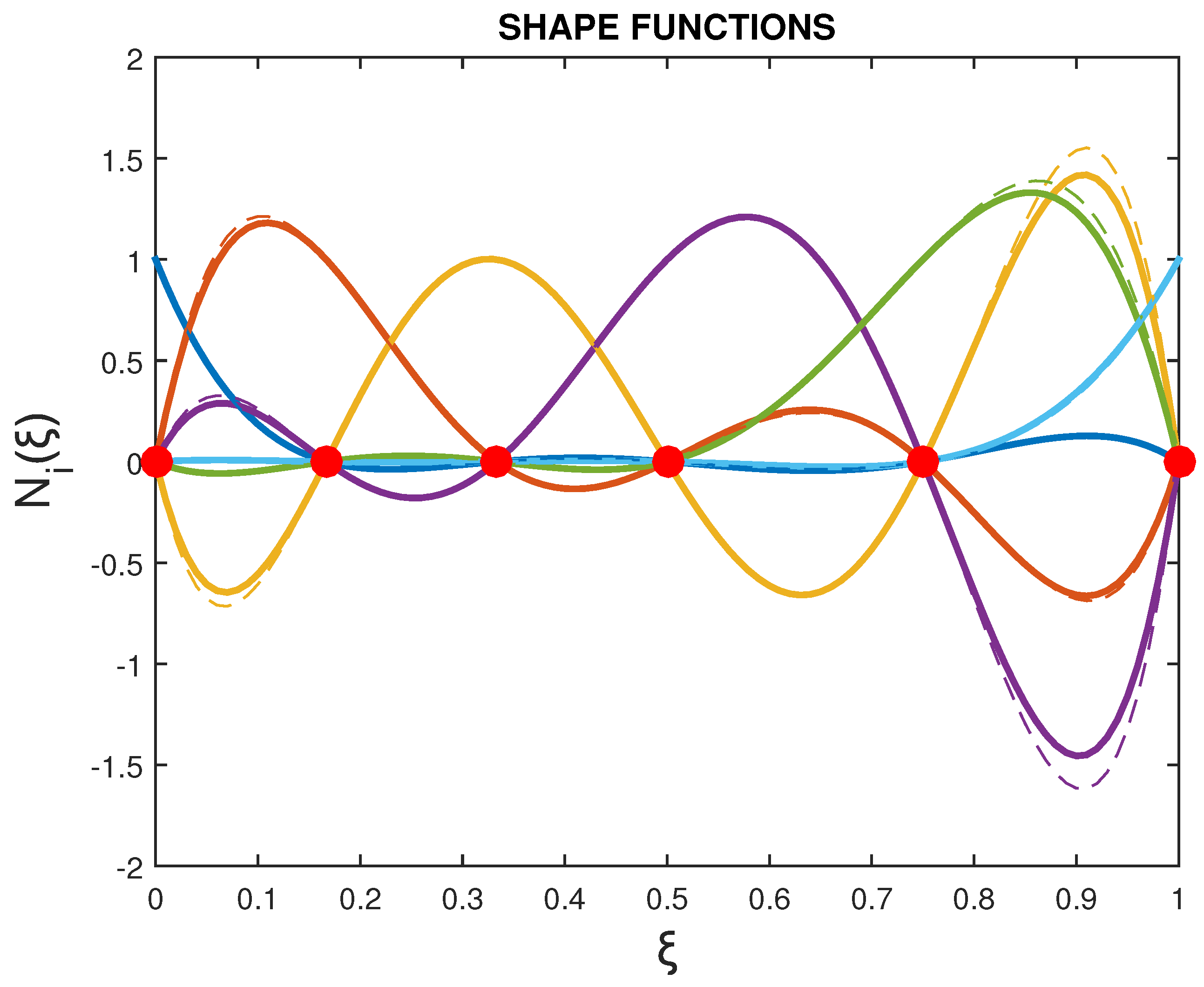
Finally, the rational and non-rational shape functions corresponding to nodal points 1–6 on the circular arc are shown in Figure 3, with identical colors used for matching curves.

3.2. Central Angle Different than 90°

The control triangle of the arc must be isosceles, the end weights can be set to 1, and the middle weight is the cosine of the angle between the chord joining the endpoints and one of the legs [17].
Therefore, if the central angle of the circular arc equals to α , to accurately represent the geometry, one choice of the weights is
w 0 = 1 , w 1 = cos α 2 , w 2 = 1 .
However, the end weights do not have to remain 1; the arc can be “reweighted” using the shape invariance ratio:
λ = w 0 w 2 w 1 2 .
For example, an equivalent choice to that of Equation (59) may be
w 0 = 2 , w 1 = 2 cos α 2 , w 2 = 2 .

4. Examples

4.1. Example 1: The Case of Degree p = 2

Let us consider a circular arc in the first quadrant, with a central angle of 90°. Considering the transformation matrix given by Equation (49) as well as the well-known column vector of weights w B = [ 1 , 2 2 , 1 ] (Ref. [17]), the Lagrangian weights are given by the column vector (see Equation (11)):
w L = T L B w B = 1 0 0 1 / 4 1 / 2 1 / 4 0 0 1 1 2 2 1 = 1 ( 1 2 + 2 4 ) 1 .
Moreover, supressing the third Cartesian coordinate ( z = 0 ), Equation (10) shows that the nodal points on the circular arc are given as
Q L w = T L B P B w = 1 0 0 1 / 4 1 / 2 1 / 4 0 0 1 1 · 1 1 · 0 2 2 · 1 2 2 · 1 1 · 0 1 · 1 = 1 0 1 + 2 4 1 + 2 4 0 1 .
To obtain the Cartesian coordinates ( x , y ) of the nodal points onto the circular arc, the entries of matrix Q L w (Equation (63)) must be divided by the corresponding elements of vector w L (Equation (62)), thus obtaining
Q L = 1 : 1 0 : 1 1 + 2 4 : ( 1 2 + 2 4 ) 1 + 2 4 : ( 1 2 + 2 4 ) 0 : 1 1 : 1 = 1 0 2 2 2 2 0 1 .
Therefore, in Equation (64), we eventually derive the ( x , y ) coordinates of the two endpoints plus the middle point of the circular arc.
Remark 4.
In the above case, where p = 2 , the nodal points on which the equivalent rational Lagrange polynomials are based have divided the circular arc in two equal parts, i.e.,  [ 0 , 1 2 ] and [ 1 2 , 1 ] .
Nevertheless, for higher degrees (i.e., p > 2 ), the nodal points are not uniformly distributed. Since the parameterization does not change with degree elevation [2], the findings of this section for p = 2 are sufficient to determine the position of the nodal points for higher degrees.
Within this context, for any polynomial degree p > 2 which is related to parameter values ξ = [ 0 , 1 p , , p 1 p , 1 ] , the nodal points are calculated through the quadratic model of this subsection as follows:
x ( ξ ) = B 0 , 2 ( ξ ) B 0 , 2 ( ξ ) + 2 2 B 1 , 2 ( ξ ) + B 2 , 2 ( ξ ) 0 1 + 2 2 B 1 , 2 ( ξ ) B 0 , 2 ( ξ ) + 2 2 B 1 , 2 ( ξ ) + B 2 , 2 ( ξ ) 0 1 + B 2 , 2 ( ξ ) B 0 , 2 ( ξ ) + 2 2 B 1 , 2 ( ξ ) + B 2 , 2 ( ξ ) 0 1 .
The results of sweeping the spectrum of polynomial degrees from p = 2 to p = 6 and applying Equation (65) to the uniform parameters ξ = [ 0 , 1 p , , p 1 p , 1 ] are listed in Table 3.

4.2. Example 2: The Case of Degree p = 3

4.2.1. Straight Line

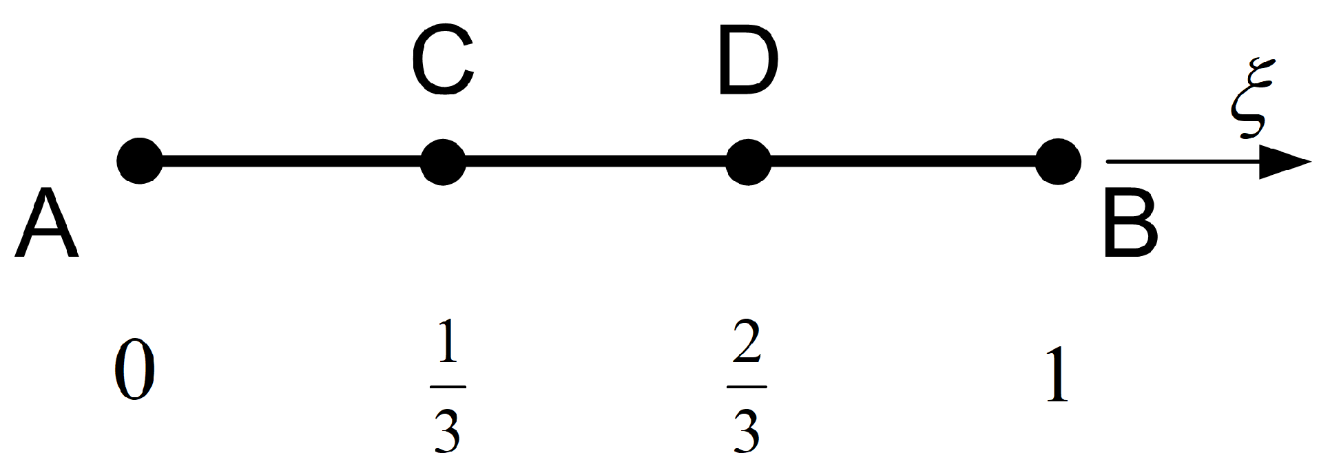
First, it is worth commenting on the representation of a straight line through rational interpolation. Within this context, let us consider a segment AB, made of points A(0,0) and B(1,1), which is uniformly subdivided in three equal parts by points C and D, as shown in Figure 4. Assuming that the parametric space along AB corresponds to the interval ξ [ 0 , 1 ] , it is reasonable to consider that points C and D correspond to ξ = 1 3 and ξ = 2 3 , respectively. Therefore, the associated Lagrange polynomials are given by
L 0 ( ξ ) = ( ξ 1 / 3 ) ( ξ 2 / 3 ) ( ξ 1 ) ( 0 1 / 3 ) ( 0 2 / 3 ) ( 0 1 ) = 9 ( ξ 1 / 3 ) ( ξ 2 / 3 ) ( ξ 1 ) L 1 ( ξ ) = ( ξ 0 ) ( ξ 2 / 3 ) ( ξ 1 ) ( 1 / 3 0 ) ( 1 / 3 2 / 3 ) ( 1 / 3 1 ) = 27 2 ξ ( ξ 2 / 3 ) ( ξ 1 ) L 2 ( ξ ) = ( ξ 0 ) ( ξ 1 / 3 ) ( ξ 1 ) ( 2 / 3 0 ) ( 2 / 3 1 / 3 ) ( 2 / 3 1 ) = 27 2 ξ ( ξ 1 / 3 ) ( ξ 1 ) L 3 ( ξ ) = ( ξ 0 ) ( ξ 1 / 3 ) ( ξ 2 / 3 ) ( 1 0 ) ( 1 1 / 3 ) ( 1 2 / 3 ) = 9 2 ξ ( ξ 1 / 3 ) ( ξ 2 / 3 ) .
Given the weights
w 0 = 1 , w 1 , w 2 , w 3 = 1 ,
associated with the points (A, C, D, B), the rational approximation is given as
x ( ξ ) = w 0 L 0 X 0 + w 1 L 1 X 1 + w 2 L 2 X 2 + w 3 L 3 X 3 w 0 L 0 + w 1 L 1 + w 2 L 2 + w 3 L 3
and
y ( ξ ) = w 0 L 0 Y 0 + w 1 L 1 Y 1 + w 2 L 2 Y 2 + w 3 L 3 Y 3 w 0 L 0 + w 1 L 1 + w 2 L 2 + w 3 L 3 .
By definition, due to the cardinality of rational shape functions, parameters ξ i = 0 , 1 3 , 2 3 , 1 correspond to points A, C, D, and B, respectively. In all cases, it is found that the whole mapping is the straight segment AB itself. For example, if the segment lies on the bisector of the right angle in the first quadrant, the nodal points are equal to each other, and thus the same rational basis functions lead to the same output ( x ( ξ ) = y ( ξ ) ).
Moreover, it was found that
  • When w 1 = w 2 , the mapping is uniform, i.e.,  x ( ξ ) = y ( ξ ) = ξ .
  • In contrast, when w 1 w 2 , the mapping is non-uniform.

4.2.2. Circular Arc of 90 °

Now, we focus on the representation of the circular arc using rational Lagrange polynomials of degree p = 3 .
While Equation (66) is still valid, in the current case—due to symmetry with respect to the bisector of first quadrant—the weights are taken as
w 0 = 1 , w 1 = w 2 , w 3 = 1 .
The question is whether it is possible to determine a unique value of the weight w 1 such that the corresponding rational Lagrange polynomials, based on the uniform nodes (A, C, D, B) in the physical space, can exactly represent the circular arc. In this regard, by means of a counterexample, we will show that this is not generally possible.
Substituting Equations (68) and (69) into the circle constraint
x ( ξ ) 2 + y ( ξ ) 2 1 = 0 ,
yields a sixth-degree polynomial in ξ , as follows:
p ( ξ ) = i = 0 6 c i ξ i 0 ,
with
c 0 = 0 ,
c 1 = 9 3 27 2 w 1 2 ,
c 2 = ( 162 81 3 ) 2 w 1 2 + ( 405 306 3 ) 4 w 1 + 20 ,
c 3 = ( 1053 3 2106 ) 4 w 1 2 + ( 513 3 594 ) 2 w 1 153 2 ,
c 4 = ( 4698 2349 3 ) 4 w 1 2 + ( 1809 1728 3 ) 4 w 1 + 279 2 ,
c 5 = 243 4 9 ( 3 2 ) w 1 2 + 18 ( 3 1 ) w 1 6 ,
c 6 = 1 4 729 ( 2 3 ) w 1 2 + 486 ( 1 3 ) w 1 + 162 .
It can be observed that the constant term c 0 vanishes a priori (Equation (73)), while the root of Equation (74) gives ( w 1 ) 1 0.9576447 . The closest root of the binomial in Equation (75) is slightly larger, ( w 1 ) 2 0.9599365 , whereas Equation (76) vanishes at a higher value, ( w 1 ) 3 0.9715457 . Equation (77) yields two complex roots, and the remaining two equations differ substantially from ( w 1 ) 1 0.9576447 . Therefore, no real value of w 1 can make all coefficients c 0 to c 6 simultaneously zero.
In conclusion,
  • It is generally not possible to represent a circular arc accurately using equidistant nodal points, even with rational Lagrange polynomials. By employing optimization techniques, where an objective function such as f ( w 1 ) = ( x 2 + y 2 1 ) 2 is minimized, a value of w 1 can be determined that approximately satisfies c i 0 for i = 1 , , 6 . Nevertheless, small deviations from the ideal circle remain (e.g., beyond the fourth decimal place).
  • In contrast, if the nodal points in the physical space are chosen at the non-equidistant positions listed in Table 3, and the corresponding weights are taken from Table 1, the circle equation ( x 2 + y 2 = 1 ) is satisfied exactly.

4.3. Example 3: The Case of Degree p = 5

Let us deal with the uniform case of p = 5 . For  0 ξ 1 , the Lagrange polynomials are as follows:
L 1 ( ξ ) = ( 625 ( ξ 1 ) ( ξ 1 / 5 ) ( ξ 2 / 5 ) ( ξ 3 / 5 ) ( ξ 4 / 5 ) ) / 24 = ( 625 ξ 5 ) / 24 + ( 625 ξ 4 ) / 8 ( 2125 ξ 3 ) / 24 + ( 375 ξ 2 ) / 8 ( 137 ξ ) / 12 + 1 , L 2 ( ξ ) = 3125 ξ ( ξ 1 ) ( ξ 2 / 5 ) ( ξ 3 / 5 ) ( ξ 4 / 5 ) ) / 24 = ( 3125 ξ 5 ) / 24 ( 4375 ξ 4 ) / 12 + ( 8875 ξ 3 ) / 24 ( 1925 ξ 2 ) / 12 + 25 ξ , L 3 ( ξ ) = 3125 ξ ( ξ 1 ) ( ξ 1 / 5 ) ( ξ 3 / 5 ) ( ξ 4 / 5 ) ) / 12 = ( 3125 ξ 5 ) / 12 + ( 8125 ξ 4 ) / 12 ( 7375 ξ 3 ) / 12 + ( 2675 ξ 2 ) / 12 25 ξ , L 4 ( ξ ) = ( 3125 ξ ( ξ 1 ) ( ξ 1 / 5 ) ( ξ 2 / 5 ) ( ξ 4 / 5 ) ) / 12 = ( 3125 ξ 5 ) / 12 625 ξ 4 + ( 6125 ξ 3 ) / 12 ( 325 ξ 2 ) / 2 + ( 50 ξ ) / 3 , L 5 ( ξ ) = ( 3125 ξ ( ξ 1 ) ( ξ 1 / 5 ) ( ξ 2 / 5 ) ( ξ 3 / 5 ) ) / 24 = ( 3125 ξ 5 ) / 24 + ( 6875 ξ 4 ) / 24 ( 5125 ξ 3 ) / 24 + ( 1525 ξ 2 ) / 24 ( 25 ξ ) / 4 , L 6 ( ξ ) = ( 625 ξ ( ξ 1 / 5 ) ( ξ 2 / 5 ) ( ξ 3 / 5 ) ( ξ 4 / 5 ) ) / 24 = ( 625 ξ 5 ) / 24 ( 625 ξ 4 ) / 12 + ( 875 ξ 3 ) / 24 ( 125 ξ 2 ) / 12 + ξ .
The Lagrange polynomials defined in Equation (80) can be combined with the nodal points Q L on the exact circular arc (for brevity, the third coordinate is omitted since z = 0 )
Q L = 1 ( 4 2 + 240 ) 257 24 2 + 45 97 54 2 20 97 64 2 15 257 0 0 ( 64 2 15 ) 257 54 2 20 97 24 2 + 45 97 4 2 + 240 257 1 ,
and the associated weights w L
w L = 1 , 17 + 4 2 25 , 13 + 6 2 25 , 13 + 6 2 25 , 17 + 4 2 25 , 1 ,
both listed in Table 3 for p = 5 . In this case, the arc is represented accurately up to the 15th decimal place, which corresponds to the precision limit of our computer.
While the aforementioned nodal coordinates in Equation (81) were obtained using the quadratic Bernstein formulation (Equation (65)), the same result can also be achieved by first computing the control points P B and the associated weights w B of the Bernstein polynomials corresponding to the degree elevation from p = 2 to p = 5 . This presentation is meaningful, as it also illustrates the general procedure in cases where the six control points are generated in an arbitrary manner (i.e., not by degree elevation, which preserves the shape, but rather by shifting the control points during the design process).
Subsequently, the transformation matrix ( T L B ) p = 5 in Equation (52) can be applied to determine the desired Q L and w L .
Within this context, the successive application of Equation (1) gives the projected coordinates P B w of the control points (not presented), while the associated weights are isolated in the following column vector (Table 1 for p = 5 ):
w B = 1 , 3 + 2 5 , 4 + 3 2 10 , 4 + 3 2 10 , 3 + 2 5 , 1 .
Applying the dehomogenization according to Equation (5), the Cartesian coordinates P B of the control points in the Bernstein representation of the quarter circle are given as follows:
P B = 1 1 3 + 3 2 4 + 3 2 1 + 3 2 4 + 3 2 2 3 + 2 0 0 2 3 + 2 1 + 3 2 4 + 3 2 3 + 3 2 4 + 3 2 1 1 .
As mentioned earlier, the two columns of P B (of size 6 × 2 ) in Equation (84) correspond to the x- and y-cordinates, respectively.
The circular arc under consideration occupies the first quadrant and is subdivided at the nodal points which correspond to the parametric vector Ξ = 0 , 1 5 , 2 5 , 3 5 , 4 5 , 1 . To determine the Cartesian coordinates of the images in the entries of set Ξ , it becomes necessary to apply the rational Bézier formula
x ( ξ ) = j = 0 5 B j , 5 ( ξ ) w B j P B j j = 0 5 B j , 5 ( ξ ) w B j , with ξ Ξ = { 0 , 1 5 , 2 5 , 3 5 , 4 5 , 1 } ,
where the coordinates P B i are given by Equation (84). The corresponding weights w B j are the entries of column vector in Equation (83).
Based on the Cartesian coordinates of nodal points Q L on the true circular arc according to Equation (85), which eventually are found to be the same as those in Equation (81), and using weights w L shown in Table 1, which are the same as those in Equation (82), the parametric equation of the circular arc is as follows:
x ( ξ ) = i = 0 5 L i , 5 ( ξ ) w L i Q L i i = 0 5 L i , 5 ( ξ ) w L i , with ξ 0 , 1 .
The interesting issue is the position of the nodal points in the Lagrangian model. While for quadratic interpolation (i.e., p = 2 ) the nodal points are the two endpoints and the middle point, in all other situations, they are arranged in a non-uniform way. For example, for the current case, where p = 5 , the polar angle for the nodal points (1 to 6 in the counter-clockwise direction) in the first quadrant is shown in Table 4. One may observe that, although  Δ ξ = 1 5 is a constant, the corresponding central angles Δ α differ from one another.

5. Spherical Cap

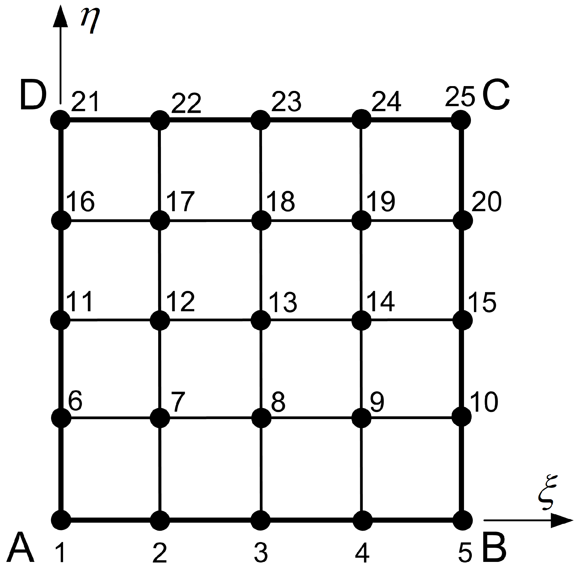
The above formulation is applicable to surfaces as well. As an example, we consider a spherical cap, which is exactly one-sixth of a unit sphere’s surface. It is known that the quadratic interpolation is not capable of accurately representing this curvilinear surface [18]. In contrast, quartic interpolation ( p = 4 ) in conjunction with 25 control points can accurately represent this cap [19] (see the parametric space in Figure 5).
Regarding the southern spherical cap, the location of 25 control points and the associated weights are available through the MATLAB function southcap=rsmak(‘southcap’). With respect to Bernstein polynomials of degree p = 4 , the Cartesian coordinates and the associated weights of control points are shown in Table 5. There, one may observe that the analytical formula is not an ideal tensor product, in the sense that the weights associated with the internal control points are not products of the corresponding boundary ones (i.e., w i j w i w j ).
By analogy to the one-dimensional procedure reported in the previous sections of this paper, the algorithm to derive the nodal points (on the true sperical surface) and the associated weights is as follows:
  • Calculate projected control points P B w and associated weights w B . This is implemented using the abovementioned built-in MATLAB function:
    southcap = rsmak ( southcap ) .
  • Create the total transformation matrix T 2 D , of size 25 × 25 (see below). In more detail, if the one-dimensional matrix T 1 D = ( T L B ) p = 4 of Equation (51) is shortly written as
    T 1 D = t 11 t 15 t 51 t 55 ,
    the 2D analog—applied to a surface patch—becomes
    T 2 D = t 11 T 1 D t 15 T 1 D t 51 T 1 D t 55 T 1 D .
  • Multiply the control points P B w by the abovementioned T 2 D and thus determine the projected nodal points Q L w :
    Q L w = T 2 D P B w .
  • Multiply the weights vector w B by the abovementioned T 2 D and thus derive the weights w L associated with Lagrange polynomials:
    w L = T 2 D w B .
  • At the end, divide the projected coordinates Q L w (Equation (89)) by the corresponding entries of w L (Equation (90)), one-to-one, and thus derive the Cartesian coordinates Q L of nodal points on the true spherical cap. Obviously, the two vectors ( Q L , w L ) are the final outcome of the proposed algorithm.
The implementation of the above algorithm to the southern spherical cap of a sphere of unit radius ( R = 1 ) gives the numerical values shown in Table 6. Based on these data, for every pair ( ξ , η ) [ 0 , 1 ] 2 , the image was found to belong to the true spherical cap (numerical error less than 10 15 ) and also coincided with the corresponding point obtained using rational Bernstein polynomials.

6. Generalization to Arbitrary Tensor-Product Surfaces

The proposed method is applicable to rational Bézier patches (or curves) and to assemblies thereof (domain decomposition). It is not applicable to B-spline patches (or curves), as explained at the end of Section 8.

6.1. General Approach

For tensor-product surfaces of arbitrary topology, the proposed method generalizes into a structured two-step procedure. The core challenge is that the mapping from the parametric ( ξ , η ) space to the physical ( x , y , z ) space is not known a priori. The solution involves determining the Cartesian coordinates of nodal points Q L (which lie on the true surface) and their associated weights w L by solving a coupled nonlinear system.
Step 1: Establish the Parametric Grid and Basis Functions
  • Define the Parametric Grid: A structured grid of ( n + 1 ) × ( m + 1 ) parameters ( ξ i , η j ) is defined in the unit square [ 0 , 1 ] × [ 0 , 1 ] . This grid establishes the topology of the Lagrange patch. The nodal parameters can be set, for instance, to  ξ nodal = [ 0 , 1 / n , , ( n 1 ) / n , 1 ] and η nodal = [ 0 , 1 / m , , ( m 1 ) / m , 1 ] for a surface of degree p = n in the ξ -direction and q = m in the η -direction. Non-uniform sets ξ nodal and η nodal are acceptable as well.
  • Construct Basis Functions: The corresponding sets of Lagrange polynomials L i ( ξ ) and L j ( η ) are constructed. These polynomials satisfy the cardinal property L i ( ξ k ) = δ i , k .
  • Initialize the Rational Basis: Rational basis functions R i , j ( ξ , η ) are formally constructed from these Lagrange polynomials and unknown weights w i , j . As an initial step for numerical solvers, all weights can be set to 1.
Step 2: Solve the Coupled Nonlinear System
The unknowns—the Cartesian coordinates of nodal points Q L i , j = ( x i , j , y i , j , z i , j ) and their associated weights w L i , j —are found by solving a system constrained by both data and the intrinsic geometry of the target surface S ( ξ , η ) . This is a constrained nonlinear optimization problem.
  • Objective Function (Data Fitting): Surface S ( ξ , η ) = i j R i , j ( ξ , η ) · Q L i , j must approximate a set of M data points P k sampled from the target surface ( P k must not be confused with control points). This leads to the objective function being minimized:
    F ( Q L , w ) = k S ( ξ k , η k ; Q L , w L ) P k 2 .
  • Nonlinear Constraints (Geometric Fidelity): Nodal points Q L i , j must satisfy the implicit equations defining the target surface’s geometry. For a surface defined by F ( x , y , z ) = 0 , this imposes the constraints
    g i , j ( Q L ) = F ( x i , j , y i , j , z i , j ) = 0 for all i , j .

6.1.1. General Algorithm

This coupled system (Equations (91) and (92)) is typically solved using a nonlinear least-squares solver (e.g., Levenberg–Marquardt [20,21]) or other large-scale nonlinear optimization techniques, where the nodal net { Q L i , j } and weights { w L i , j } are (equally) the optimization variables. Within the context of MATLAB software, a useful function for this purpose is fsolve.

6.1.2. Efficient Algorithm

The fully coupled nonlinear optimization, while robust, can be computationally intensive. In practice, we often employ a computationally efficient iterative refinement procedure that decouples the problem into a sequence of simpler sub-problems. This approach is numerically stable and converges rapidly for well-behaved geometries.
Our algorithm proceeds as follows:
Initialization: We initialize all weights to w i , j = 1 , reducing the rational Lagrange formulation to a standard polynomial Lagrange one.
Iterative Loop:
(a) 
Linear Nodal Point Solve: With the weights fixed at their current values, the determination of the nodal points Q L i , j becomes a linear least-squares problem. We solve this efficiently for the best-fit nodal net.
(b) 
Nonlinear Weight Update: Holding the newly computed nodal points constant, we perform a lightweight nonlinear optimization to update only the weights. This step adjusts the rational basis functions to better match the intrinsic curvature of the target surface.
(c) 
Check Convergence: We iterate between steps (a) and (b) until the change in the solution is negligible.
Advantages of this Approach:
  • Efficiency: It leverages highly optimized linear algebra solvers for the most expensive step (finding the nodal net).
  • Robustness: It avoids the pitfalls of initializing a full nonlinear solver with a poor guess. Starting with weights=1 provides a sensible, neutral starting point.
  • Theoretical Foundation: This method can be viewed as a variant of the Gauss–Newton algorithm for nonlinear least squares, applied specifically to the structure of our problem.

6.2. Illustrative Example: A 90-Degree Circular Arc

This example serves as a rapid simplification (analog) of the theory to better understand the general two algorithms proposed in Section 6.1.1 and Section 6.1.2. Instead of a surface S ( ξ , η ) , here we deal with a curve C ( ξ ) (with analytical solution cited in Section 4.1).
Let us consider a circular arc ( Q L 1 , Q L 2 , Q L 3 ), with endpoints
Q L 1 = ( x L 1 , y L 1 ) = ( 1 , 0 ) , and Q L 3 = ( x L 3 , y L 3 ) = ( 0 , 1 ) ,
whereas the weights associated with endpoints Q L 1 and Q L 3 are
w L 1 = w L 3 = 1 .
The three unknown quantities are the two Cartesian coordinates of nodal point Q L 2 ( x L 2 , y L 2 ) , which is supposed to be unknown (i.e., it is not a priori known that it lies at the middle of the circular arc), plus its associated weight w L 2 .
First, we establish the parametric grid ξ 1 = 0 , ξ 2 = 1 2 , ξ 3 = 1 and thus construct the non-rational Lagrange polynomials,
L 1 ( ξ ) = ( 2 ξ 2 3 ξ + 1 ) , L 2 ( ξ ) = ( 4 ξ 2 + 4 ξ ) , L 3 ( ξ ) = ( 2 ξ 2 ξ ) ,
as well as the rational ones:
R 1 ( ξ ) = w L 1 L 1 ( ξ ) w L 1 L 1 ( ξ ) + w L 2 L 2 ( ξ ) + w L 3 L 3 ( ξ ) , R 2 ( ξ ) = w L 2 L 2 ( ξ ) w L 1 L 1 ( ξ ) + w L 2 L 2 ( ξ ) + w L 3 L 3 ( ξ ) , R 3 ( ξ ) = w L 3 L 3 ( ξ ) w L 1 L 1 ( ξ ) + w L 2 L 2 ( ξ ) + w L 3 L 3 ( ξ ) .
Second, we choose an arbitrary data point (or ‘test point’) on the true boundary C ( ξ ) , for example, at ξ = 1 3 , and then apply the isoparametric conditions:
x test = R 1 ( 1 3 ) x L 1 + R 2 ( 1 3 ) x L 2 + R 3 ( 1 3 ) x L 3 ,
y test = R 1 ( 1 3 ) y L 1 + R 2 ( 1 3 ) y L 2 + R 3 ( 1 3 ) y L 3 .
Note that even though we are dealing with a circular arc, due to the non-rational Lagrange formulation (as also happens with non-rational Bernstein polynomials), the data point at ξ = 1 3 does not generally correspond to polar angle θ = π 6 . This in turn means that the Cartesian coordinates ( x test , y test ) are still unknown. The pair of Equations (95) and (96) is the analog of Equation (91), whereas the analog of Equation (92), i.e., the circle constraint, provides the third, necessary equation:
x L 2 2 + y L 2 2 = 1 .
After manipulation, the system of Equations (95)–(97) becomes
w L 2 ( x L 2 0.872260419102717 ) + 0.140967447612160 = 0 ,
w L 2 ( y L 2 0.489041676410868 ) 0.186130209551359 = 0 ,
x L 2 2 + y L 2 2 1 = 0
One may easily verify that the exact analytical solution (Section 4.1), i.e.,
w L 2 = 2 + 2 4 = 0.853553390593274 , x L 2 = y L 2 = 2 2 = 0.707106781186548 ,
fufils all three equalities, i.e., the system of Equations (98)–(100).
On the other hand, the resulting three equations (i.e., Equations (95)–(97)) in three unknowns ( x L 2 , y L 2 , w L 2 ) form a nonlinear system, which is solved numerically, implementing one of the techniques described below.
Within this context, following Section 6.1.1, we can implement the MATLAB function fsolv and thus determine the numerical solution after seven iterations. With default tolerance ( 1 × 10 6 ), the numerical solution is ( x L 2 = 0.707106334280096 , y L 2 = 0.707107241220445 , w L 2 = 0.853550498699083 ) . Actually, one may observe that deviation of the calculated values ( x L 2 , y L 2 ) from the exact analytical solution (Equation (101)) occurs after the sixth decimal place. By further decreasing the tolerance, it was found that the accuracy improves.
Alternatively, following Section 6.1.2, we can initially assume that w L 2 = 1 , and thus Equation (98) gives x L 2 0.731292971490557 , whereas Equation (99) gives y L 2 0.675171885962227 . This result means that the estimated nodal point does not belong to the circle because it violates the constraint, since
x L 2 2 + y L 2 2 = ( 0.731292971490557 ) 2 + ( 0.675171885962227 ) 2 = 0.990646485745279 < 1 .
Next, we enforce the geometric constraint (unit circle) by increasing both Cartesian coordinates using the factor
λ = 0 . 990646485745279 0.995312255397912 ,
and thus the updated Cartesian coordinates become
x L 2 , n e w = 0.731292971490557 / λ = 0.734737231983742 ,
y L 2 , n e w = 0.675171885962227 / λ = 0.678351826073218 .
First technique: Average. For the sake of brevity, henceforth, we omit the subscript ‘L’ in Cartesian coordinate x L 2 and associated weight w L 2 , formerly used as an emphasis that we are dealing with Lagrange polynomials and nodal points. Substituting Equation (104) into Equation (98), which also is shortly written as
w 2 = b 1 / ( x 2 a 1 ) ,
with ( a 1 = 0.872260419102717 , b 1 = 0.140967447612160 ), we derive a new weight w 2 .
Also, substituting Equation (105) into Equation (99), which is also shortly written as:
w 2 = b 2 / ( y 2 a 2 ) ,
with ( a 2 = 0.489041676410868 , b 2 = 0.186130209551359 ), we derive a new weight w 2 .
Of course, we can take the average  ( w 2 , n e w = ( w 2 + w 2 ) / 2 ) of these two values and repeate the above procedure until convergence is achieved.
Second technique: Least-Squares Blend. The conflicting weight estimates are reconciled by solving for w new , which minimizes the L 2 -norm of residual A w b 2 , where
A = x 2 a 1 y 2 a 2 , b = b 1 b 2
The solution is computed efficiently using MATLAB’s backslash operator: w_new = A \ b.
Third technique: Nonlinear Optimization. The optimal weight w new * is determined by solving the nonlinear least-squares problem:
min w w ( x 2 a 1 ) + b 1 2 + w ( y 2 a 2 ) b 2 2
using MATLAB’s lsqnonlin solver with initial guess w old . The implementation is
  f = @(w) [w*(x_2 - a1) + b1; w*(y_2 - a2) - b2];
      w_new = lsqnonlin(f, w_old);
The above procedure of the third technique can be easily extended to surfaces as well.
Fourth technique: Analytical solution. To come to an end, we also present a fourth technique, which, however, is trivial, tailored for this particular problem of the circular arc. Solving Equation (98) in x 2 and Equation (99) in y 2 , and then substituting both of them in Equation (100), we obtain a nonlinear equation in w 2 :
0.872260419102717 0.140967447612160 w 2 2 + 0.489041676410868 + 0.186130209551359 w 2 2 = 1
Solving this equation numerically gives the exact solution:
w 2 = 0.853553390593274
x 2 = 0.707106781186548
y 2 = 0.707106781186548

6.3. Remarks on Trivial Cases

Remark 5.
For free-form surfaces, the projected control points P B w and the associated weights w B are typically provided by the CAD system. Therefore, if they can be organized in an assembly of rational Bézier patches, the same procedure as in the case of the aforementioned spherical cap can be applied.
Remark 6.
It is worth noting that explicit rational Bézier (or NURBS) representations of classical quadrics (e.g., circle, ellipse, sphere, cylinder, cone, paraboloid, hyperboloid) are well established, with control points and associated weights available in closed form [1,2]. Therefore, the same procedure as that applied to the aforementioned spherical cap can be directly extended to these quadrics. General quadrics in an arbitrary position can then be obtained through suitable affine or projective transformations.

7. A Boundary-Value Problem

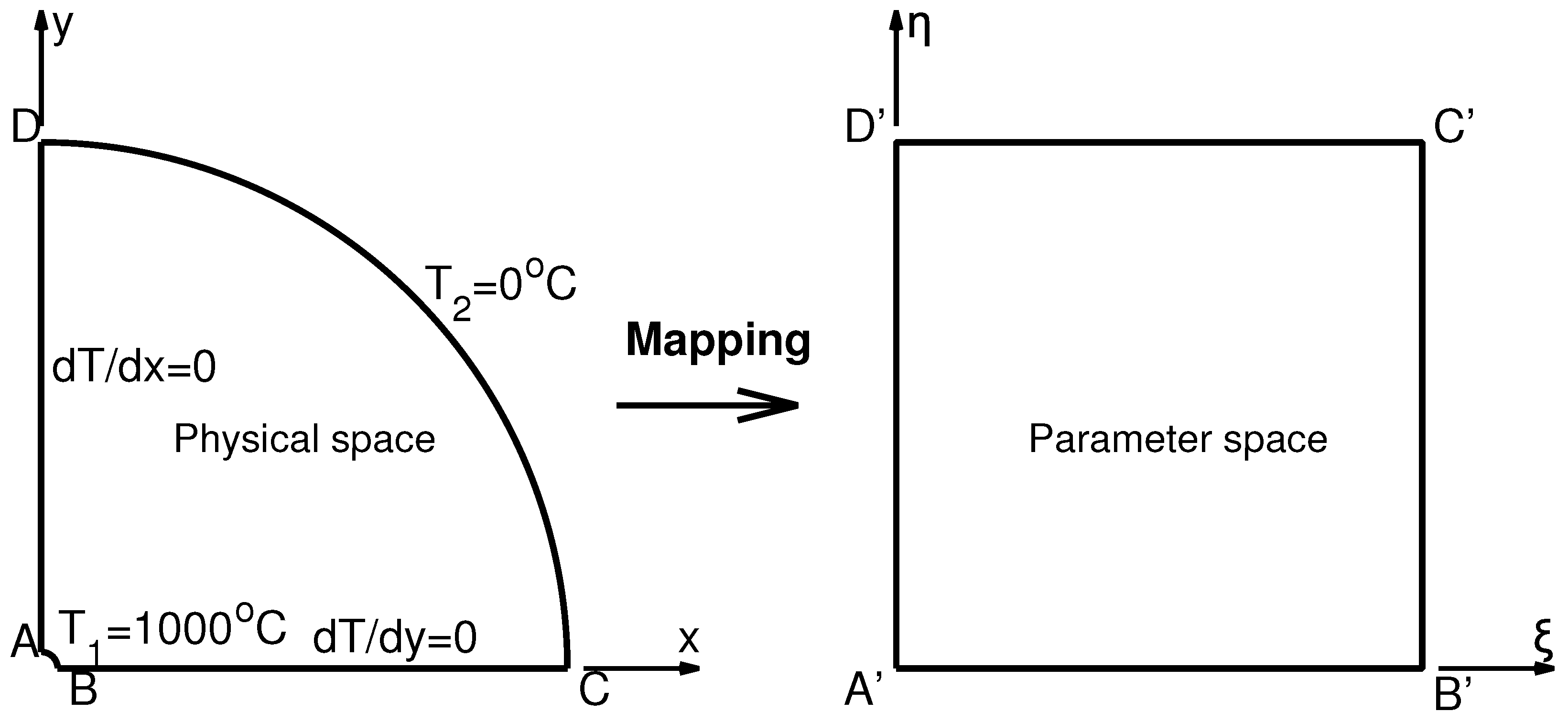
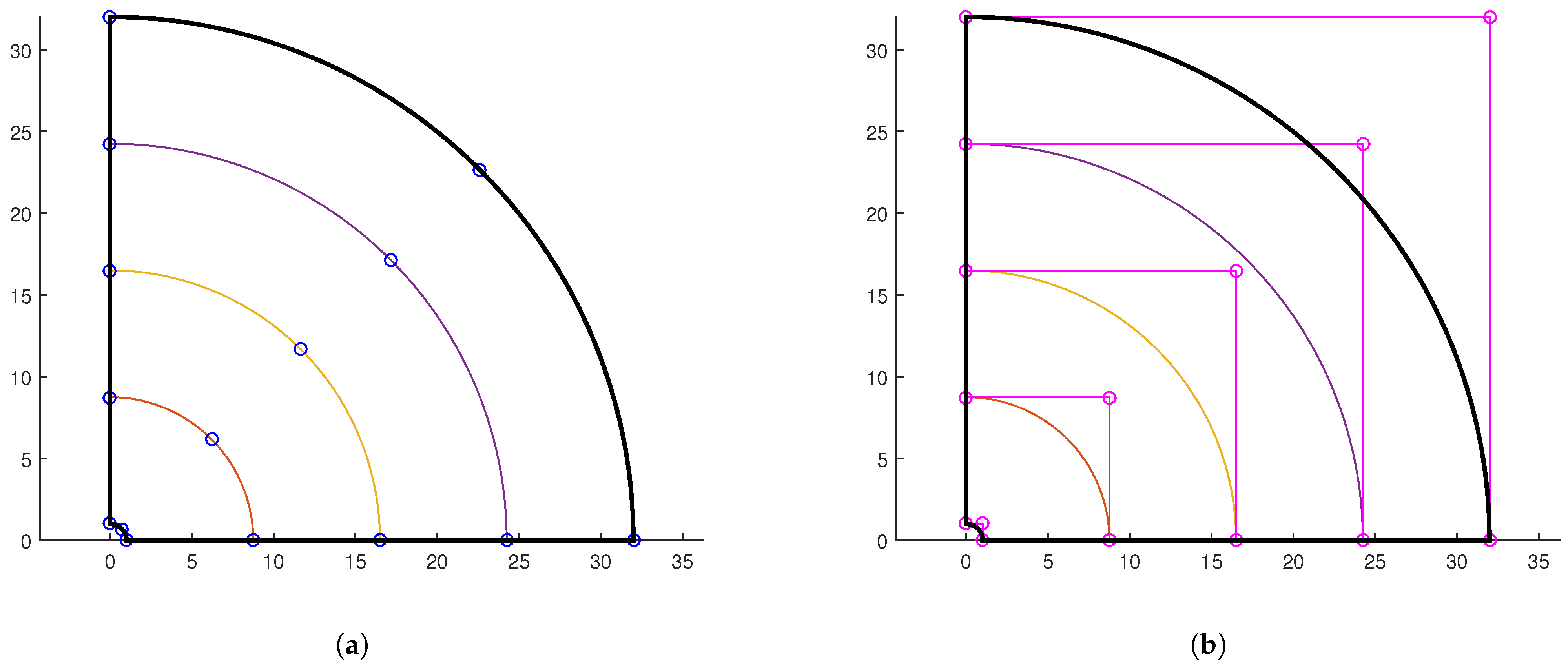
In this section, we study the heat flow (i.e., the numerical solution of Laplace equation 2 T = 0 ) into the quarter of an annulus A B C D , with internal radius R 1 = 1 and external radius R 2 = 32 (Figure 6, left). The corresponding temperatures on the circular edges ( A B and D C ) of the annulus are T 1 = 1000 °C (along A B ) and T 2 = 0 °C (along D C ), whereas the flux perpendicular to the straight edges ( A D and B C ) vanishes ( U / n = 0 ), where n is the outward normal unit vector (x or y accordingly, as shown in Figure 6, left). The physical domain A B C D is mapped to a unit reference square ( A B C D , as exaggeratedly shown in Figure 6, right), which serves as a parametric domain. In more detail, the circular arc A B of the physical space corresponds to edge A B (i.e., the ξ -axis) of the parametric space, whereas straight edge A D corresponds to edge A D (i.e., the η -axis) of the parametric domain. Therefore, A B C D is considered as a single patch (a rational Bézier or rational Lagrange macroelement), suitable for isogeometric analysis.
In terms of radius r (with R 1 r R 2 ), the analytical solution is given by [22]
T exact ( r ) = T 1 + ( T 2 T 1 ) log R 2 R 1 log r R 1 .
The quality of numerical solution T calculated in domain Ω is presented by the L 2 error norm (in percent), which is defined as follows:
L 2 = Ω T calculated T exact 2 d Ω Ω T exact 2 d Ω × 100 ( % ) .
Two alternative formulations were implemented, as described in the following subsections.

7.1. The Proposed Approach

Each of the two circular arcs (in the ξ direction) was divided into two equal parts using three nodes on the true boundary, whereas the weights associated with quadratic Lagrange polynomials were w L = [ w 1 , w 2 , w 3 ] = [ 1 , 1 2 + 2 4 , 1 ] (see Table 1 for p = 2 ).
In terms of the usual uniform quadratic Lagrange polynomials, L j , 2 ( ξ ) , j = 1 , 2 , 3 ,
L 1 , 2 ( ξ ) = 2 ( ξ 1 2 ) ( ξ 1 ) , L 2 , 2 ( ξ ) = 4 ξ ( ξ 1 ) , L 3 , 2 ( ξ ) = 2 ξ ( ξ 1 2 ) ,
the corresponding rational Lagrange polynomials are given as
L ^ i , 2 ( ξ ) = w i L i , 2 ( ξ ) j = 1 3 w j L j , 2 ( ξ ) , j = 1 , 2 , 3 .
Moreover, the number n y of uniform sudivisions in the radial ( η ) direction varied among 1 and 25 (i.e., degree 1 p y = n y 23 ), and the relevant usual uniform Lagrange polynomials, L j , p y ( η ) , j = 1 , , n y + 1 , were combined with unit weights.
Following the standard FEM approach, the numerical solution within the entire patch is written as a tensor product of rational and non-rational Lagrange polynomials, as follows:
T ( ξ , η ) = i = 1 3 j = 1 n y + 1 L ^ i , 2 ( ξ ) L j , p y ( η ) .
Obviously, since the nodal points are arranged in triplets along the n y + 1 circular arcs (as shown in Figure 7a for n y = 4 ), for any given value n y , the total number of nodes in the model, which lie on the true boundary and the interior, will be
n nodes = 3 ( n y + 1 ) .

7.2. Standard IGA Approach

The standard IGA is based on control points, as shown in Figure 7b for n y = 4 . Each circular arc is determined by three control points: two at the ends and a third at the intersection of the two tangents at these ends (outside the curve). The quadratic Bernstein polynomials B j , 2 ( ξ ) , j = 1 , 2 , 3 , are
B 1 , 2 ( ξ ) = ( 1 ξ ) 2 , B 2 , 2 ( ξ ) = 2 ( 1 ξ ) ξ , B 3 , 2 ( ξ ) = ξ 2 ,
whereas the corresponding weights are w B = [ w 1 , w 2 , w 3 ] = [ 1 , 2 2 , 1 ] (see, [17]).
Based on the usual quadratic Bernstein polynomials of Equation (118), the corresponding rational Bernstein polynomials are given as
R i , 2 ( ξ ) = w i B i , 2 ( ξ ) j = 1 3 w j B j , 2 ( ξ ) , j = 1 , 2 , 3 .
Considering the η -direction, which is modeled with n y + 1 control points, the usual Bernstein polynomials B j , p y ( η ) of degree p y = n y are employed.
Therefore, the numerical solution within the entire patch is written as a tensor product of rational and non-rational Bernstein polynomials, as follows:
T ( ξ , η ) = i = 1 3 j = 1 n y + 1 R i , 2 ( ξ ) B j , p y ( η ) .

7.3. Results

All computations were performed using MATLAB version R2025a.
Identical numerical results were obtained using both the proposed Lagrange-based scheme (Equation (117), Figure 7a) and the standard Bernstein-based IGA formulation (Equation (120), Figure 7b). The calculated L 2 error norm (Equation (114), in percent) is shown in Figure 8.
It may be observed in Figure 8 that up to p y = 23 , the convergence is monotonic, after which it increases slightly. It is also worth noting that even for the coarsest model (i.e., n y = 1 ), the exact analytical value of area
A exact = π R 2 2 R 1 2 4 ,
was accurately approximated (up to the 15th decimal place) by numerically performing the integral of the determinant of Jacobian matrix, i.e.,
A = d A = det ( J ) d ξ d η .

8. Discussion

It was shown that the set of weights associated with Bernstein polynomials and control points, which determine a certain rational Bézier curve C ( ξ ) , can be successfully replaced by another set of weights associated with Lagrange polynomials of the same degree and nodal points on the same true curve.
The key point is to determine the transformation matrix within the rational Bézier curve, T L B , which relates the vector of Bernstein polynomials (B) to that of Lagrange polynomials (L). This relationship depends on the parametric location of the nodal points, thus enabling uniform and non-uniform nodal positions. It is noted that—given the parametric location of the nodal points—the matrix T L B is the same, i.e., independent of the location of the control points. Therefore, to each vector P B w of control points there corresponds a unique vector Q L w of nodal points on the true curve (surface).
Starting with the consituents of the rational Bernstein–Bézier curve, i.e., control points P B and weights w B , we can easily determine projected nodal points Q L w and their weights w L in the Lagrangian formulation and eventually find the nodal points Q L on true curve C ( ξ ) . Based on them, for any arbitrary parameter ξ , we can calculate the associated rational Lagrange polynomials and then apply series expansion (isoparametric superposition) to determine the corresponding point x ( ξ ) . It was found that the relevant approximation accurately represents a circular arc (maximum error less than 10 15 ).
The same concept is applicable to a surface (curvilinear patch) as well. As an example, we considered the spherical cap, which refers to one-sixth of a sphere. It is well known that this is accurately represented by a rational Bézier surface of degree p = 4 , which is not an ideal tensor product. The latter means that the weights of the interior satisfy inequality w i j w i w j ; therefore, since 5 control points exist in each direction, the denominator of the normalization will be a sum of 25 terms. A generic expression was presented to construct the total transformation matrix (of size 25 × 25 ) in terms of the one-dimensional transformation matrix T L B (of size 5 × 5 ) along any edge of the quadrilateral patch. Next, the twenty-five nodal points on the true surface were determined, and for each parametric pair ( ξ , η ) , the spherical cap was accurately represented (with a maximum deviation of less than 10 15 ).
An additional advantage of using nodal points on the true boundary of the physical domain is the fact that stiffness and mass matrices directly refer to the nodal values, U i , and thus, boundary conditions are easily imposed. Relevant numerical results—using rational Lagrange polynomials—are presented in Section 7, where an excellent convergence is reported for the numerical solution of a boundary-value problem governed by the Laplace equation. In addition, it is worth mentioning that identical numerical results were found when rational Bernstein–Bézier polynomials were implemented for the same problem.
The proposed theory is limited to rational Bézier patches or to assemblies of such patches with C 0 interelement continuity. In this case, each Bézier element possesses its own transformation matrix ( T L B ) e , and thus, the nodal coordinates (together with the associated weights) are determined at the element level.
Due to the local support of B-splines (each basis being nonzero over only p + 1 consecutive spans), adjacent spans always share p basis functions. For example, with p = 2 and Ξ = [ 0 , 0 , 0 , 1 2 , 1 , 1 , 1 ] , the first span [ 0 , 1 2 ] involves ( N 1 , N 2 , N 3 ) and the second span [ 1 2 , 1 ] involves ( N 2 , N 3 , N 4 ) , so the two elements cannot be treated in isolation.

9. Conclusions

The usual representation of smooth patches through tensor-product rational Bernstein–Bézier polynomials can be equivalently replaced by rational Lagrange polynomials. To maintain this numerical equivalence, it is necessary to implement transformation matrices associated with the two mutually perpendicular body-fitted directions and thus to determine nodal points on the true boundary together with the corresponding weights. The geometrical concept was applied to a circular arc and a spherical cap, whereas a boundary-value problem governed by the Laplace equation was successfully solved for a quarter of an annulus.

Funding

This research received no external funding.

Data Availability Statement

The raw data supporting the conclusions of this article will be made available by the author on request.

Conflicts of Interest

The author declares no conflicts of interest.

References

  1. Farin, G. Curves and Surfaces for CAGD: A Practical Guide, 5th ed.; Morgan Kaufmann: San Francisco, CA, USA, 2002. [Google Scholar]
  2. Piegl, L.; Tiller, W. The NURBS Book, 2nd ed.; Springer: Berlin/Heidelberg, Germany, 1997. [Google Scholar]
  3. Hoschek, J.; Lasser, D. Fundamentals of Computer Aided Geometric Design, 2nd ed.; A.K. Peters: Wellesley, MA, USA, 1996. [Google Scholar]
  4. Hughes, T.J.R.; Cottrell, J.A.; Bazilevs, Y. Isogeometric analysis: CAD, finite elements, NURBS, exact geometry and mesh refinement. Comput. Methods Appl. Mech. Eng. 2005, 194, 4135–4195. [Google Scholar] [CrossRef]
  5. Desiderio, L.; D’Inverno, G.A.; Sampoli, M.L.; Sestini, A. Hierarchical matrices for 3D Helmholtz problems in the multi-patch IgA-BEM setting. Eng. Comput. 2025, 41, 2021–2042. [Google Scholar] [CrossRef]
  6. Schillinger, D.; Ruthala, P.K.; Nguyen, L.H. Lagrange extraction and projection for NURBS basis functions: A direct link between isogeometric and standard nodal finite element formulations. Int. J. Numer. Methods Eng. 2016, 108, 515–534. [Google Scholar] [CrossRef]
  7. Liu, B.; Xing, Y.; Wang, Z.; Lu, X.; Sun, H. Non-uniform rational Lagrange functions and its applications to isogeometric analysis of in-plane and flexural vibration of thin plates. Comput. Methods Appl. Mech. Eng. 2017, 321, 173–208. [Google Scholar] [CrossRef]
  8. Lu, L.Z. Adaptive Polynomial Approximation to Circular Arcs. Appl. Mech. Mater. 2011, 50, 678–682. [Google Scholar] [CrossRef]
  9. Vavpetič, A. Optimal parametric interpolants of circular arcs. Comput. Aided Geom. Des. 2020, 80, 101891. [Google Scholar] [CrossRef]
  10. Vavpetič, A.; Žagar, E. A general framework for the optimal approximation of circular arcs by parametric polynomial curves. J. Comput. Appl. Math. 2019, 345, 146–158. [Google Scholar] [CrossRef]
  11. Vavpetič, A.; Žagar, E. On optimal polynomial geometric interpolation of circular arcs according to the Hausdorff distance. J. Comput. Appl. Math. 2021, 392, 113491. [Google Scholar] [CrossRef]
  12. De Boor, C. A Practical Guide to Splines, Revised ed.; Applied Mathematical Sciences; Springer: New York, NY, USA, 2001. [Google Scholar]
  13. Patera, A.T. A spectral element method for fluid dynamics: Laminar flow in a channel expansion. J. Comput. Phys. 1984, 54, 468–488. [Google Scholar] [CrossRef]
  14. Pozrikidis, C. Introduction to Finite and Spectral Element Methods Using MATLAB, 2nd ed.; CRC Press: Boca-Raton, FL, USA, 2014. [Google Scholar]
  15. Eisenträger, S.; Eisenträger, J.; Gravenkamp, H.; Provatidis, C.G. High order transition elements: The xNy-element concept-part II: Dynamics. Comput. Methods Appl. Mech. Eng. 2021, 387, 114145. [Google Scholar] [CrossRef]
  16. Provatidis, C.G. Precursors of Isogeometric Analysis: Finite Elements, Boundary Elements, and Collocation Methods; Solid Mechanics and Its Applications; Springer International Publishing: Cham, Switzerland, 2019. [Google Scholar] [CrossRef]
  17. Piegl, L.; Tiller, W. A menagerie of rational B-spline circles. IEEE Comput. Graph. Appl. 1989, 9, 48–56. [Google Scholar] [CrossRef]
  18. Provatidis, C. How accurately can spherical caps be represented by rational quadratic polynomials? WSEAS Trans. Circuits Syst. 2021, 20, 139–146. [Google Scholar] [CrossRef]
  19. Cobb, J.E. Tiling the Sphere with Rational Bézier Patches, TR UUCS-88-009. 1988. Available online: https://core.ac.uk/download/pdf/276277507.pdf (accessed on 9 May 2025).
  20. Levenberg, K. A Method for the Solution of Certain Problems in Least-Squares. Q. Appl. Math. 1944, 2, 164–168. [Google Scholar] [CrossRef]
  21. Marquardt, D. An Algorithm for Least-squares Estimation of Nonlinear Parameters. SIAM J. Appl. Math. 1963, 11, 431–441. [Google Scholar] [CrossRef]
  22. Carslaw, H.S.; Jaeger, J.C. Conduct. Heat Solids, 2nd ed.; Oxford University Press: Oxford, UK, 1969. [Google Scholar]
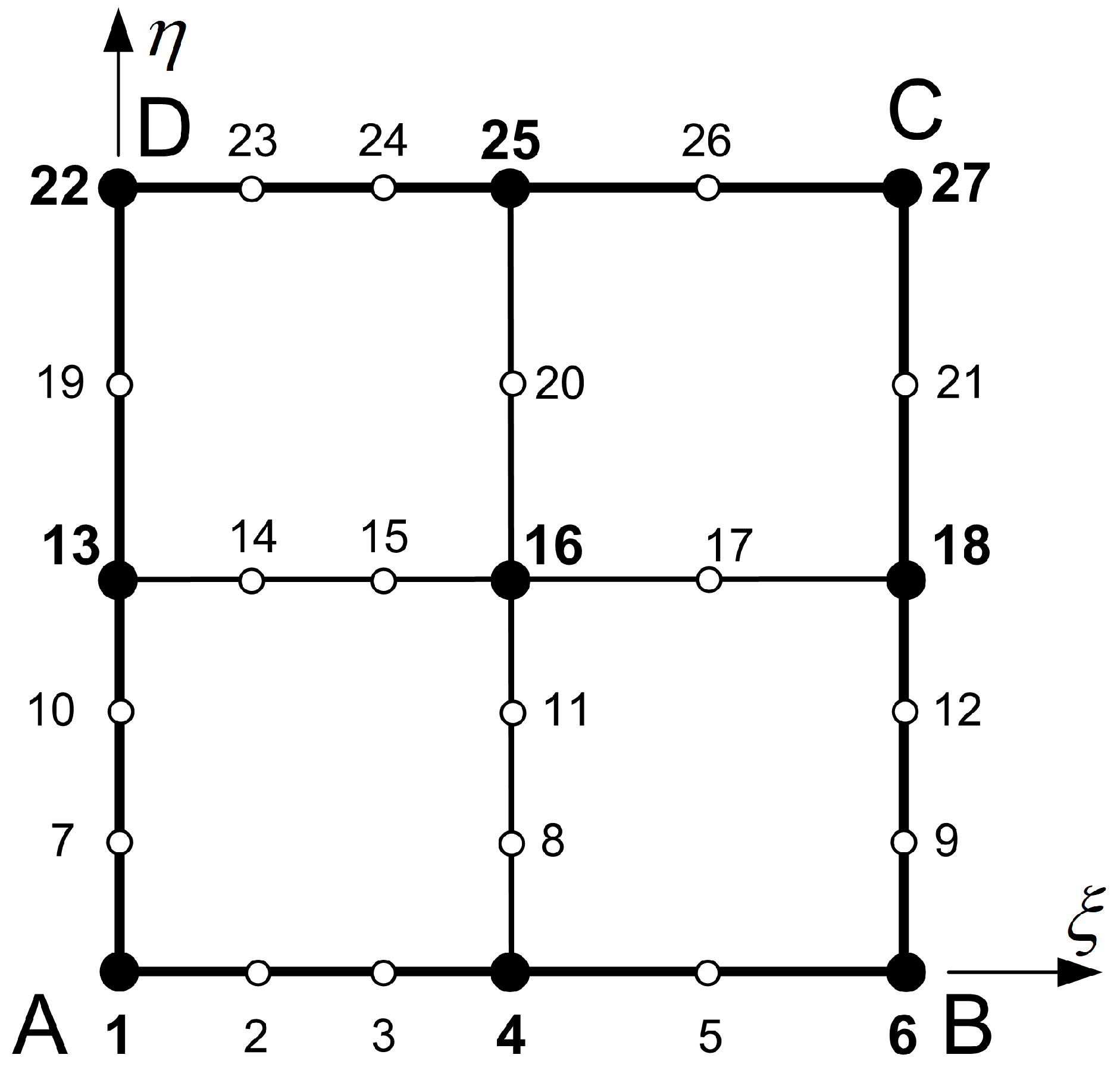
Figure 1. Twenty-seven node classical transfinite element ABCD.
Mathematics 13 03239 g001
Figure 2. Modelling of edge AB in the 27-node classical transfinite element (see Figure 1).
Mathematics 13 03239 g002
Figure 3. Shape functions for rational (solid lines) and standard non-rational (dashed lines) Lagrange polynomials (corresponding to the nodal points on edge AB in Figure 1).
Mathematics 13 03239 g003
Figure 4. Uniform subdivision of straight segment.
Mathematics 13 03239 g004
Figure 5. Numbering of control points in the reference square ABCD.
Mathematics 13 03239 g005
Figure 6. Problem definition for the quarter of an annulus, which is mapped to a unit square.
Mathematics 13 03239 g006
Figure 7. Discretization of the quarter-annulus ( n x = 2 , n y = 4 ) using (a) weighted (rational) Lagrange polynomials and (b) rational Bernstein–Bézier polynomials.
Mathematics 13 03239 g007
Figure 8. Convergence quality for the quarter of an annulus.
Mathematics 13 03239 g008
Table 1. Weights w B and w L for the quarter of a circle.
Degree (p)Bernstein (Equation (3))Lagrange (Equation (11))
2 ( 1 , 2 2 , 1 ) ( 1 , 2 + 2 4 , 1 )
3 ( 1 , 1 + 2 3 , 1 + 2 3 , 1 ) ( 1 , 15 + 6 2 27 , 15 + 6 2 27 , 1 )
4 ( 1 , 2 + 2 4 , 1 + 2 3 , 2 + 2 4 , 1 ) ( 1 , 10 + 3 2 16 , 2 + 2 4 , 10 + 3 2 16 , 1 )
5 ( 1 , 3 + 2 5 , 4 + 3 2 10 , 4 + 3 2 10 , 3 + 2 5 , 1 ) ( 1 , 17 + 4 2 25 , 13 + 6 2 25 , 13 + 6 2 25 , 17 + 4 2 25 , 1 )
6 ( 1 , 4 + 2 6 , 7 + 4 2 15 , 4 + 3 2 10 , 7 + 4 2 15 , 4 + 2 6 , 1 ) ( 1 , 26 + 5 2 36 , 5 + 2 2 9 , 2 + 2 4 , 5 + 2 2 9 , 26 + 5 2 36 , 1 )
Table 2. Central angles α i and β i , with  i = 1 , , 5 (in degrees) associated with the endpoints of ξ i [ 0 , 1 ] .
ξ i 0 1 6 2 6 3 6 3 4 1
α i 14.125815.151815.722423.401821.5982
β i 14.125815.151815.722423.401821.5982
Table 3. Nodal coordinates Q L on the circular arc for polynomial degree p at uniform parameter values ξ .
pCoordinates
Node-1Node-2Node-3Node-4Node-5Node-6Node-7
21 2 2 0
0 2 2 1
31 ( 2 2 + 12 ) 17 ( 8 2 3 ) 17 0
0 ( 8 2 3 ) 17 ( 2 2 + 12 ) 17 1
41 3 2 82 + 36 41 2 2 27 2 82 4 41 0
0 27 2 82 4 41 2 2 3 2 82 + 36 41 1
51 ( 4 2 + 240 ) 257 24 2 + 45 97 54 2 20 97 64 2 15 257 0
0 ( 64 2 15 ) 257 54 2 20 97 24 2 + 45 97 4 2 + 240 257 1
61 5 2 626 + 300 313 2 2 17 + 12 17 2 2 ( 8 2 3 ) 17 125 2 626 12 313 0
0 125 2 626 12 313 8 2 17 3 17 2 2 ( 2 2 + 12 ) 17 5 2 626 + 300 313 1
Table 4. Polar angle (in degrees) for the quarter of a circle ( p = 5 ).
Nodal Point
123456
17.0863 ° 35.5286 ° 54.4714 ° 72.9137 ° 90 °
Table 5. Cartesian coordinates and weights associated with the 25 control points on the southern spherical cap of a unit sphere ( p = 4 ).
CoordinatesWeights
Pointxyzw
1−0.5773503−0.5773503−0.57735035.0717968
2−0.3128762−0.7095873−0.70958734.5200421
30.0000000−0.7540208−0.75402084.3572656
40.3128762−0.7095873−0.70958734.5200421
50.5773503−0.5773503−0.57735035.0717968
6−0.7095873−0.3128762−0.70958734.5200421
7−0.4133641−0.4133641−1.00000003.8660254
80.0000000−0.4573041−1.12004623.6449237
90.4133641−0.4133641−1.00000003.8660254
100.7095873−0.3128762−0.70958734.5200421
11−0.75402080.0000000−0.75402084.3572656
12−0.45730410.0000000−1.12004623.6449237
130.00000000.0000000−1.27983323.4045574
140.45730410.0000000−1.12004623.6449237
150.75402080.0000000−0.75402084.3572656
16−0.70958730.3128762−0.70958734.5200421
17−0.41336410.4133641−1.00000003.8660254
180.00000000.4573041−1.12004623.6449237
190.41336410.4133641−1.00000003.8660254
200.70958730.3128762−0.70958734.5200421
21−0.57735030.5773503−0.57735035.0717968
22−0.31287620.7095873−0.70958734.5200421
230.00000000.7540208−0.75402084.3572656
240.31287620.7095873−0.70958734.5200421
250.57735030.5773503−0.57735035.0717968
Table 6. Cartesian coordinates and weights associated with the 25 nodal points on the southern spherical cap of a unit sphere ( p = 4 ).
CoordinatesWeight
Pointxyzw
1−0.5773503−0.5773503−0.57735035.0717968
2−0.3100080−0.6722704−0.67227044.6624403
30.0000000−0.7071068−0.70710684.5279702
40.3100080−0.6722704−0.67227044.6624403
50.5773503−0.5773503−0.57735035.0717968
6−0.6722704−0.3100080−0.67227044.6624403
7−0.3729805−0.3729805−0.84957114.1882599
8−0.0000000−0.3971773−0.91774194.0306408
90.3729805−0.3729805−0.84957114.1882599
100.6722704−0.3100080−0.67227044.6624403
11−0.7071068−0.0000000−0.70710684.5279702
12−0.39717730.0000000−0.91774194.0306408
13−0.0000000−0.0000000−1.00000003.8648644
140.39717730.0000000−0.91774194.0306408
150.7071068−0.0000000−0.70710684.5279702
16−0.67227040.3100080−0.67227044.6624403
17−0.37298050.3729805−0.84957114.1882599
18−0.00000000.3971773−0.91774194.0306408
190.37298050.3729805−0.84957114.1882599
200.67227040.3100080−0.67227044.6624403
21−0.57735030.5773503−0.57735035.0717968
22−0.31000800.6722704−0.67227044.6624403
230.00000000.7071068−0.70710684.5279702
240.31000800.6722704−0.67227044.6624403
250.57735030.5773503−0.57735035.0717968
Disclaimer/Publisher’s Note: The statements, opinions and data contained in all publications are solely those of the individual author(s) and contributor(s) and not of MDPI and/or the editor(s). MDPI and/or the editor(s) disclaim responsibility for any injury to people or property resulting from any ideas, methods, instructions or products referred to in the content.