Assessing Air-Pocket Pressure Peaks During Water Filling Operations Using Dimensionless Equations

Abstract

Air pockets can become trapped at high points in pipelines with irregular profiles, particularly during service interruptions. The resulting issues, primarily caused by peak pressures generated during pipeline filling, are a well-documented topic in the literature. However, it is surprising that this subject has not received comprehensive attention. Using a model developed by the authors, this paper identifies the key parameters that define the phenomenon, presenting equations in a dimensionless format. The main advantage of this study lies in the ability to easily compute pressure surges without the need to solve a complex system of differential and algebraic equations. Numerous cases of filling operations were analysed to obtain dimensionless charts that can be used by water utilities to compute pressure surges during filling operations. Additionally, it provides charts that facilitate the rapid and reasonably accurate estimation of peak pressures. Depending on their transient characteristics, pressure peaks are either slow or fast, with separate charts provided for each type. A practical application involving a water pipeline with an irregular profile demonstrates the model’s effectiveness, showing strong agreement between calculated and chart-predicted (proposed methodology) values. This research provides water utilities with the ability to select the appropriate pipe’s resistance class required for water distribution systems by calculating the pressure peak value that may occur during filling procedures.

1. Introduction

Understanding air–water interactions in pressurised hydraulic systems is critical for preventing pipeline failures caused by pressure surges [1,2,3]. Water utilities must pay particular attention to filling operations, as large air pockets often remain trapped within hydraulic systems before the process begins [4]. The water column can compress the air phase as the system is filled, leading to rapid or slow pressure surges. These operations must be accurately predicted to prevent undesirable pressure peaks [5,6]. Air pockets tend to accumulate at high points in hydraulic systems with irregular profiles, making the installation of air valves at these locations a common and effective recommendation [7,8,9].

Other factors requiring careful consideration include the operation of regulating valves, which should be manoeuvred as slowly as possible to minimise pressure surges [10], and the energy source driving the system [5]. Interestingly, smaller air pockets along hydraulic installations increase the risk of pressure surges, necessitating thorough drainage during emptying operations to mitigate this effect [4,11].

In reference [12], the development of predictive curves for pressure surges is presented, as cited by reference [10]. Reference [12] presented a chart that overestimates pressure peaks in practical scenarios due to its inability to account for the movement of blocking columns. Additionally, the chart fails to predict pressure surges in pump-powered systems. Other works, including those by reference [13] and reference [14], further examine this phenomenon, highlighting its potential dangers and advocating for the installation of air valves to vent the air phase.

Based on these studies, in reference [5], the development of a mathematical model that incorporates the movement of blocking columns in water pipelines with irregular profiles is presented. This approach employs the rigid water-column model, as air elasticity far exceeds the combined elasticity of the water phase and pipeline. References [6,15] presented a comparable solution to this issue, utilising the elastic water-column model. Both models yield similar predictions for key variables, including air-pocket pressure, the location of air–water interfaces, and water velocity, making them suitable for scenarios where air valves are absent or fail due to maintenance issues.

More recently, Coronado-Hernández et al. (2019) [16] and Zhou et al. (2019) [17] proposed enhanced models for air expelled through air valves, employing rigid and elastic water-column frameworks. These models have been validated using diverse experimental setups in recent years. Additionally, the problem can now be addressed using Computational Fluid Dynamics (CFD) models, which allow for detailed simulations of real-world scenarios in existing installations and experimental facilities [18,19,20]. However, CFD simulations can take months to complete. To avoid this problem, water utilities must acquire quantum computing technology [21]. Nevertheless, modelling the internal geometries of air and regulating valves presents inherent complexities, introducing certain uncertainties into simulations. During filling operations, it is of utmost importance to identify the polytropic evolution (typically considered as an intermediate evolution with an exponent coefficient of 1.2) [4], pipeline characteristics (such as absolute roughness, pipe length, internal pipe diameters, and longitudinal slopes) [22], as well as the definition of initial conditions for starting up, using recommended values suggested by the American Water Works Association (AWWA) [9], local regulations, or existing publications [23].

The authors have been working for many years on hydraulic transients involving entrapped air, particularly focusing on the study of filling and emptying processes in pressurised hydraulic systems [4], developing mathematical models to analyse these phenomena, which have been validated through various experimental measurements. These mathematical models consist of a set of differential equation systems whose resolution is not straightforward.

This study’s innovation lies in accounting for the mobility of air–water interfaces, which closes the gap between theoretical models and real-world behaviour. The model employs a system of equations that can describe the motion of the filling column and blocking columns.

This study, based on the model above, aims to (i) identify the key parameters influencing pressure peaks, (ii) advance the theoretical understanding of the problem, and (iii) create charts to predict pressure surges in practical installations with reasonable accuracy. This research presents a tool that water utilities can use to compute pressure surges that occur during filling operations in irregular profile pipelines, since it provides a novel scheme for computing the maximum peaks of absolute pressure without solving complex equations of this issue [5,24].

2. Materials and Methods

The authors have developed a system of differential–algebraic equations to examine the evolution of air–water interfaces during the filling operations of a pipeline with an irregular profile, accounting for $n$ entrapped air pockets [5,16,25]. The flow is supplied by an energy source, such as a reservoir or pump, and includes a valve to regulate the flow rate. It comprises $2+3n$ equations, matched by the same number of unknown variables: three for each entrapped air pocket with their corresponding blocking columns (air–water interface position, $x_{i }$, air-pocket pressure, $p_i^{\mathrm{*}}$, and water velocity in the blocking column, $v_i$), as well as two additional variables for the filling column (its length, $L$, and water velocity, $v$). Figure 1 presents the scheme for a filling operation, which contains the main parameters and variables of the issue.

Figure 2 illustrates the methodology employed in this research. This research’s first stage involves converting physical equations into dimensionless forms, as detailed in Section 2. Based on this analysis, the second stage focuses on practical charts that aid in predicting the filling process with entrapped air pockets. Section 3 elaborates on the development of these charts, which are crucial, as the parametrisation provided can be applied to any water installation to determine the maximum pressure surges. Finally, Section 4 addresses the third stage, showcasing a practical application to a water installation.

2.1. Dimensionless Variables

The reference scales used in the non-dimensionalization of this set of equations are presented in

Table 1. Dimensionless variables.

Dimensionless Variable	Variable Scale
Pressure head:	$H_e^{*}={\displaystyle \frac{p_e^{*}}{\gamma }}=H_r+H_{atm}^{*}+H_p\left(Q=0\right), (11)$
$h^{*}={\displaystyle \frac{p_0^{*}}{p_e^{*}}}={\displaystyle \frac{H_0^{*}}{H_e^{*}}}, (1)$
Air-pocket pressure head $i$:
$h_i^{*}={\displaystyle \frac{p_i^{*}}{p_e^{*}}}={\displaystyle \frac{H_i^{*}}{H_e^{*}}}, (2)$
Filling-column velocity:	$v_e=\sqrt{2g\left(H_e^{*}-H_{atm}^{*}\right)}, (12)$
$v={\displaystyle \frac{v}{v_e}}, (3)$
Blocking-column velocity $i$:
$v_i={\displaystyle \frac{v_i}{v_e}}, (4)$
Filling-column length:	$L_e=L_{air\mathrm{1,0}}, (13)$
$l={\displaystyle \frac{L}{L_e}}, (5)$
Position of a blocking column $i$:
$X_i={\displaystyle \frac{x_i}{L_e}}, (6)$
Gravity term of the filling column:	Equation (11)
$∆\zeta ={\displaystyle \frac{∆z}{H_e^{*}}}, (7)$
Gravity term of a blocking column $i$:
$∆{\zeta }_i={\displaystyle \frac{∆z_{b,i}}{H_e^{*}}}, (8)$
Air-pocket volume $i$:	$$\begin{gathered} {\forall }_e={\forall }_{\mathrm{1,0}}=\left(x_{\mathrm{1,0}}-L_0\right)\cdot A, (14) \\ {L}_e=L_{air\mathrm{1,0}}, (15) \end{gathered}$$
${\phi }_t={\displaystyle \frac{{\forall }_i}{{\forall }_e}}={\displaystyle \frac{L_{air,i}}{L_e}}, (9)$
Time:	$T_e={\displaystyle \frac{L_e}{v_e}}={\displaystyle \frac{L_{air\mathrm{1,0}}}{\sqrt{2g\left(H_e^{*}-H_{atm}^{*}\right)}}}, (16)$
$\tau ={\displaystyle \frac{t}{T_e}}, (10)$

. These dimensionless variables are obtained by dividing the studied variable by a reference value.

2.2. Dimensionless Parameters

The dimensionless parameters were considered to establish a set of dimensionless equations, presented in

Table 2. Dimensionless parameters.

Parameter	Equation
Inertial scale	${\mathsf{\Pi }}_i={\displaystyle \frac{v_e^2}{g{H}_e^{\mathrm{*}}}}=2\left(1-{\displaystyle \frac{H_{atm}^{\mathrm{*}}}{H_e^{\mathrm{*}}}}\right)=2-{\displaystyle \frac{2}{{\mathsf{\Pi }}_m}}, \left(17\right)$
	whose value tends to 2 for powerful energy sources $\left(H_e^{\mathrm{*}} \gg H_{atm}^{\mathrm{*}}\right)$. The energy parameter is yielding by ${\mathsf{\Pi }}_m=H_e^{*}/H_{atm}^{*}$.
Friction scale	${\mathsf{\Pi }}_f={\displaystyle \frac{f{v}_e^2{L}_e}{2gD{H}_e^{\mathrm{*}}}}={\displaystyle \frac{f{L}_e}{D}}\left(1-{\displaystyle \frac{1}{{\mathsf{\Pi }}_m}}\right), (18)$
	Whose value tends to be the Martin parameter ${\displaystyle \frac{f\cdot L_e}{D}}$ [12] if $H_e^{\mathrm{*}} \gg H_{atm}^{\mathrm{*}}$; that is, when the energy parameter is ${\mathsf{\Pi }}_m$, it is big.
Parameters of water columns	(a) Blocking column $i$: ${\beta }_i={\displaystyle \frac{L_{b,i}}{L_e}}, (19)$ (b) Filling column: $\beta ={\displaystyle \frac{L}{L_e}}, (20)$ (c) Filling column (initial): ${\beta }_0={\displaystyle \frac{L_0}{L_e}}, (21)$

Note that $\beta$ values change over time, so they are not strict parameters and are irrelevant to computing pressure surges. This simplification has been considered for the current analysis.

. The dimensionless equations are formulated in terms of the dimensionless variables, where the parameters appear by deriving the equations.

The combination of ${\beta }_i$, $\beta$, and ${\beta }_0$ with friction and inertia scale parameters (Table 2), ${\mathsf{\Pi }}_f$ and ${\mathsf{\Pi }}_i$, results in the total friction and inertia parameter for the blocking columns, as follows:

$${\mathsf{\Pi }}_{f,i}={\mathsf{\Pi }}_f\cdot {\beta }_i,$$

(22)

$${\mathsf{\Pi }}_{i,i}={\mathsf{\Pi }}_i\cdot {\beta }_i,$$

(23)

In addition, the gravity terms represented by $∆\zeta$ and $∆{\zeta }_i$ play an essential role in determining pressure surges. When the peak is abrupt and occurs rapidly, the influence of $∆\zeta$ variation is minimal, making geometric similarity relatively insignificant. Conversely, when the peak gradually unfolds more slowly, this variable becomes the primary factor of pressure surges’ occurrence. Then, the profile parameter is defined as follows [24]:

$${\delta }_p={\displaystyle \frac{L_{p \mathrm{sen} }{\theta }_p}{H_e^{\mathrm{*}}}},$$

(24)

Finally, the parameter ${\alpha }_i$ relates the blocking-column capability versus the capacity to store the system’s energy-blocking column/air pocket [24].

$${\alpha }_i={\displaystyle \frac{L_{b,i}}{L_{air i,0}}},$$

(25)

The parameters ${\alpha }_i$ and ${\beta }_i$ are equal for the first entrapped air pocket.

2.3. Dimensionless Equations

The original equations were transformed into dimensionless equations based on dimensionless parameters and variables [5,16].

Table 3. Dimensionless equations.

Original Equation *	Dimensionless Equation
Filling Column (2 Equations)
1.- Rigid model equation for the filling column
${\displaystyle \frac{dv}{dt}}={\displaystyle \frac{p_0^{*}-p_1^{*}}{\rho L}}-g{\displaystyle \frac{\Delta z}{L}}-{\displaystyle \frac{fv\left|v\right|}{2D}}, (26)$	$h^{*}-h_1^{*}=\left({\mathsf{\Pi }}_i \beta \right){\displaystyle \frac{d\nu }{d\tau }}+\Delta \zeta +\left({\mathsf{\Pi }}_f \beta \right) \nu \left|\nu \right|, (31)$
2.- Water–air interface position for the filling column
$L=L_0+{\int }_0^{t}v dt, (27)$	$l={\beta }_0+{\int }_0^{\tau }vd\tau , (32)$
$n$ Blocking Columns/Air Pockets ($3n$ equations)
3.- Rigid model equation for blocking column $i \left(i = 1, 2, \dots , n\right)$
${\displaystyle \frac{d{v}_i}{dt}}={\displaystyle \frac{p_i^{*}-p_{i+1}^{*}}{\rho L_{b,i}}}-g{\displaystyle \frac{\Delta z_{b,i}}{L_{b,i}}}-{\displaystyle \frac{f{v}_i\left|v_i\right|}{2D}}, (28)$	$h_i^{*}-h_{i+1}^{*}=\left({\mathsf{\Pi }}_i {\beta }_i\right){\displaystyle \frac{d{\nu }_i}{d\tau }}+\Delta {\zeta }_i+\left({\mathsf{\Pi }}_f {\beta }_i\right) {\nu }_i\left|{\nu }_i\right|, (33)$
	Where for the last blocking column $\left(i = n\right)$, must be replaced $h_{n+1}^{*} = h_{atm}^{*}$
4.- Entrapped air pocket $i \left(i = 1, 2, \dots , n\right)$
$p_i^{*}\cdot {\left(x_i-x_{i-1}-L_{bi-1}\right)}^n=p_{i,0}\cdot {\left(x_{i,0}-x_{i-\mathrm{1,0}}-L_{bi-1}\right)}^n, (29)$	$h_i^{*}{\phi }_i^n={\displaystyle \frac{1}{{\mathsf{\Pi }}_m}}{\left({\displaystyle \frac{{\beta }_i}{{\alpha }_i}}\right)}^n, (34)$
5.- Water–air interface position for the blocking column $i \left(i = 1, 2, \dots , n\right)$
${\displaystyle \frac{d{x}_i}{dt}}=v_i, (30)$	${\displaystyle \frac{d{\phi }_i}{d\tau }}=v_i-v_{i-1}, (35)$
	being $v_0=v$ for the first trapped air pocket $\left(i = 1\right)$

* Note: details of original equations can be found in reference [5].

presents the results obtained.

2.4. Dimensionless Initial and Boundary Conditions

2.4.1. Initial Conditions $\left(\mathrm{t}=0\right)$

Under the system consideration, the following initial conditions were defined:

(a)

Filling column:

$$v\left(0\right)=0 , l\left(0\right)={\displaystyle \frac{L_0}{L_e}}={\beta }_0 ,$$

(36)

(b)

Blocking column $i/$entrapped air pocket $i$:

$$v_i\left(0\right)=0 , h_i^{\mathrm{*}}\left(0\right)={\displaystyle \frac{H_i^{\mathrm{*}}\left(0\right)}{H_e^{\mathrm{*}}}}={\displaystyle \frac{H_{i,0}^{\mathrm{*}}}{H_e^{\mathrm{*}}}}={\displaystyle \frac{H_{atm}^{\mathrm{*}}}{H_e^{\mathrm{*}}}} , {\phi }_i\left(0\right)={\displaystyle \frac{{\forall }_i\left(0\right)}{{\forall }_e}}={\displaystyle \frac{{\forall }_{i,0}}{{\forall }_e}} ,$$

(37)

2.4.2. Boundary Conditions

Equation (38) represents the energy source, which is the origin of the movement. It greatly influences the development of fast peaks, while it gives way to gravitational effects as far as slow peaks are concerned. Two parameters define their characteristics:

$$\mathrm{At} x=0 h_1^{\mathrm{*}}={\displaystyle \frac{H_r+H_{atm}^{\mathrm{*}}+H_p\left(Q\right)}{H_e^{\mathrm{*}}}} ,$$

(38)

$$\mathrm{At} x=x_n+L_{b,n}{h}_{n+1}^{\mathrm{*}}=h_{atm}^{\mathrm{*}} ,$$

(39)

-

Boundary energy (motor) parameter

$${\mathsf{\Pi }}_m={\displaystyle \frac{H_e^{\mathrm{*}}}{H_{atm}^{\mathrm{*}}}} ,$$

(40)

-

The boundary shape parameter, $\mu$, which considers the relationship $H-Q$ characterising the source of energy. For a pump, for which $H_p=A_p-C_p{Q}^2$, $\mu$ is defined as:

$$\mu =\sqrt{{\displaystyle \frac{\frac{A_p}{H_0}}{\frac{A_p}{H_0}-1}}}=\sqrt{{\displaystyle \frac{\frac{C_p\cdot Q_0^2}{H_0}+1}{\frac{C_p\cdot Q_0^2}{H_0}}}} ,$$

(41)

where $H_0$ and $Q_0$ are the steady-state delivery head and flowrate, respectively. For a reservoir, $C_p$ = 0 or, equivalently, $\mu =\infty$.

3. Pressure Surges and Characteristics Parameters

3.1. Parametrization for Slow and Rapid Air-Pocket Pressure Peaks

The set of Equations (31)–(35), the initial conditions (Equations (36) and (37)) and their boundary conditions (Equations (38) and (39)), together with the remainder of data, especially the pipeline profile defined by Equation (24), completely define the problem under consideration. Since the variables are dimensionless, the results obtained for specific parameters are universally valid. The exceptions are the gravitational terms $∆\zeta$, which cannot be considered in this parametric study since they characterise each profile. Nevertheless, their behaviour in extreme cases of interest is perfectly defined and does not pose unique difficulties in solving the problems. Thus, the parameters that define the pressure peaks for a given air pocket depend on its position within the system ($i$ = 1, 2, …, $n$). For a generic $i$, they are:

• Filling-column parameter ${\beta }_0$, Equation (32).
• Two parameters for each blocking column upstream of air pocket $i$, Equation (4): ${\mathsf{\Pi }}_{i,i}$ and ${\mathsf{\Pi }}_{f,i}$, defined by Equations (22) and (23).
• One parameter (observe that ${\beta }_i$ is included in ${\mathsf{\Pi }}_{i,i}$ and ${\mathsf{\Pi }}_{f,i}$) for each air pocket upstream of air pocket $i$, Equation (34): ${\alpha }_i$.
• One parameter standard to all the air pockets: the polytropic coefficient $n$.
• Two parameters characterising the source of energy, ${\mathsf{\Pi }}_m$ and $\mu$, and one parameter for every reach $p$ with no zero slope, ${\delta }_p$, forcing the layout. Geometry constitutes the drawback of an utterly general study. As seen later, considering only the corresponding ${\delta }_p$ to the reach where the air pocket descends gives reasonably good accuracy. Thus, as far as boundary and geometric parameters are concerned (parameters not included explicitly in the equations of the system), three parameters are enough for our study: ${\mathsf{\Pi }}_m$, $\mu$, and ${\delta }_p$.

Summing up, including the geometric parameter ${\delta }_p$ for the simplified layout, three boundary parameters, ${\mathsf{\Pi }}_m$, $\mu$, and ${\delta }_p$, two system parameters, ${\beta }_0$ and $n$, together with three characteristic parameters of each blocking column/air pocket upstream of air pocket $i$ under study, ${\mathsf{\Pi }}_{i,i}$, ${\mathsf{\Pi }}_{f,i}$, and ${\mathsf{\alpha }}_i$, must be considered. So, to study the first air pocket, eight parameters are needed, eleven for the second, and so on. Nevertheless, after solving the complete problem, only a few have significance regarding the pressure peak under study. The main criterion for their selection is the velocity of the transient generating the peak. Therefore, these parameters can be organised according to three cases:

• The case of very fast peaks, which is only possible for the first air pocket ($i$ = 1). They are generated by short transients, requiring high sources of energy (say ${\mathsf{\Pi }}_m$ ≥ 5) that, acting violently due to the sudden opening of the delivery valve (Figure 2), must overcome low initial inertia (${\beta }_0$ → 0). This makes the gravitational effects irrelevant so that ${\delta }_p$ has negligible contribution.
• The case of slow peaks is generated after the compression of an air pocket in the range of minutes. They are typical of air pockets far away from the source of energy (i ≥ 2), but also possible for the first air pocket if ${\mathsf{\Pi }}_m$ is small (around ${\mathsf{\Pi }}_m$ ≤ 1.5) or ${\beta }_0$ big (significant initial inertia). With ${\mathsf{\Pi }}_m$ being so small, it loses relevance in front of ${\delta }_p$.
• The intermediate pressure peaks, which value both effects, the driving source of energy (${\mathsf{\Pi }}_m$, $\mu$) and the gravitational effects induced by the profile (${\delta }_p$), contribute significantly.

In what follows, we will refer to the extreme cases a and b, since they offer the possibility of a more straightforward analysis and, at the same time, are susceptible to excellent physical interpretations. Case a is nevertheless the most relevant, due to the importance of the peak pressures generated. The maximum pressures for case b are frequently lower than the steady-state pressure, since they occur at the geometrical minimum of the pipeline, where steady-state pressures take their maximum.

3.1.1. Parameters for Fast Air-Pocket Pressure Peaks

Fast peaks are generated in a few seconds by an essential source of energy (${\mathsf{\Pi }}_m\ge 5$) that drives a liquid column of low initial inertia (${\beta }_0\to 0$). The short time in which the transient develops does not allow the blocking column to move significantly, so ${\mathsf{\Pi }}_{i,1}$ y ${\mathsf{\Pi }}_{f,1}$ become irrelevant. The same happens with the gravitational parameter; consequently, ${\delta }_p$ can also be ignored. Thus, only five out of the eight parameters deserve consideration: ${\beta }_0, n, {\beta }_1={\alpha }_1, {\mathsf{\Pi }}_m$, and $\mu$.

If the filling column initially has a short length, then it is verified ${\beta }_0\cong 0$ (the most critical scenario). In this case, the most significant parameters that influence the value $H_{max}^{\mathrm{*}}$ is yielded by:

$${\displaystyle \frac{H_{max}^{*}}{H_e^{*}}}=F\left({\mathsf{\Pi }}_m,{\beta }_1,\mu ,n\right) ,$$

(42)

3.1.2. Parameters for Slow Air-Pocket Pressure Peaks

If the transient is long, in the order of minutes, the air is slowly compressed, allowing the blocking column to move. Typically, this is the case of the air pockets from the second one on ($i\ge 2$), because of the high inertia of the compressed blocking column upstream of the air pocket. As said before, the first pocket can also be compressed slowly if ${\beta }_0$ is large and the initial power of the source of energy is small (${\mathsf{\Pi }}_m\le 1.5$). The solution to the problem shows that the peaks occur at the instant the blocking column immediately upstream of the air pocket under consideration reaches the geometric relative minimum, after descending the reach $p$. In this case, the relevant driving parameter is the profile parameter (${\delta }_p)$ instead of ${\mathsf{\Pi }}_m$ and $\mu$; though, in some instances, their contribution cannot be neglected. This simplification, among others, is responsible for the lower accuracy of predictions for slow peaks, on average, concerning those for fast peaks.

Since the number of parameters necessary to assess slow peaks for an air pocket is significant (inertia and friction parameters of the upstream and blocking columns), performing an analysis without neglecting some of them is not feasible. Such an analysis, depending on the velocity of the columns and the rapidity of the transient, cannot be accurate enough. Parameters ${\alpha }_i$ corresponding to the air pockets upstream of the one under study are also neglected, since, once established, the movement is transmitted with negligible pressure fluctuations. In summary, only three parameters, namely $n$, ${\alpha }_i$, and ${\delta }_p$, are considered to assess slow peaks. The results obtained are much less accurate than those for fast peaks, which can be reasonably estimated since their hypotheses are acceptably valid.

After all these simplifications of the problem posed, the most significant parameters that influence the value $H_{max,i}^{\mathrm{*}}$ are expressed as follows:

$${\displaystyle \frac{H_{max,i}^{*}}{H_e^{*}}}=F\left({\alpha }_i,{\delta }_p,n\right) ,$$

(43)

3.2. Parametric Analysis

Once the parameters characterising the problem are identified, elaborating charts to assess their magnitude is a straightforward task, since as many simulations as necessary, using the complete model, can be performed. In all cases, the influence of the polytropic coefficient, $n$, is important. Although the charts have been developed for $n$ = 1.2 [5,12], laboratory tests are underway for a more precise value. The ordinate axis corresponds to the value ${\displaystyle \raisebox{1ex}{$H_{max}^{*}$}\!\left/ \!\raisebox{-1ex}{$H_e^{*}$}\right.}$, from which it is straightforward to determine the maximum pressure.

3.2.1. Charts to Determine Fast Air-Pocket Pressure Peaks

Having fixed the polytropic index ($n=1.2$) and considering ${\beta }_0\cong 0$, three parameters are relevant for fast peaks: ${\beta }_1={\alpha }_1$, ${\mathsf{\Pi }}_m$ and $\mu$. Figure 3 presents three charts corresponding to ${\mathsf{\Pi }}_m$ = 10, 20, and 30 for ${\alpha }_1$ values within the interval 0–48 and shape factors $\mu$ = 2, 5, 10, 15, 20, and ∞.

3.2.2. Charts to Determine Slow Air-Pocket Pressure Peaks

Taking $n=1.2$ again, this chart gives the relationship between ${\alpha }_i$ and $H_{max}^{\mathrm{*}}/H_e^{\mathrm{*}}$ * for different values of ${\delta }_p$. Figure 4 presents the chart to determine pressure peaks $H_{max}^{\mathrm{*}}/H_e^{\mathrm{*}}$ for values of ${\alpha }_i$ in the interval 0–16 and profile parameter values ${\delta }_p$ = 0.2, 0.5, 1, 1.5, 2, 3, and 5.

3.3. Boundary Between Fast and Slow Air-Pocket Pressure Peaks

Defining a boundary between the two types of pressure peaks is essential. The types of air-pocket pressure peaks depend on air-pocket size (characterised by the parameter ${\beta }_1$), and the parameters ${\mathsf{\Pi }}_m$ and $\mu$, presented in Figure 5. A polytropic coefficient $n=1.2$ has been selected, since it is used in many practical applications.

After identifying the most significant dimensionless parameters for estimating pressure peaks, numerous cases were processed to generate these dimensionless charts (see Figure 3, Figure 4 and Figure 5). This information can be used to calculate the maximum pressure peaks occurring during transient events in filling manoeuvres.

The use of Figure 3, Figure 4 and Figure 5 involves calculating the values of $\alpha$ and ${\delta }_p$, from which the ratio ${\displaystyle \raisebox{1ex}{$H_{max}^{*}$}\!\left/ \!\raisebox{-1ex}{$H_e^{*}$}\right.}$ is obtained. Once $H_e^{*}$ is determined, $H_{max}^{*}$ can be calculated.

4. Practical Application

The proposed dimensionless equations were employed considering the installation dataset in Figure 6. The installation has an upstream reservoir with a different water elevation of 50 m from the downstream reservoir. The total length of the water installation ($L_{Total}$) is 1430 m, with an internal pipe diameter ($D$) of 150 mm and a friction factor of 0.018. Water installations with similar characteristics pertain to operations that water utilities are required to manage in municipalities. The filling operation is conducted in this water installation. The steady-state condition is reached with a water velocity of 2.38 m/s.

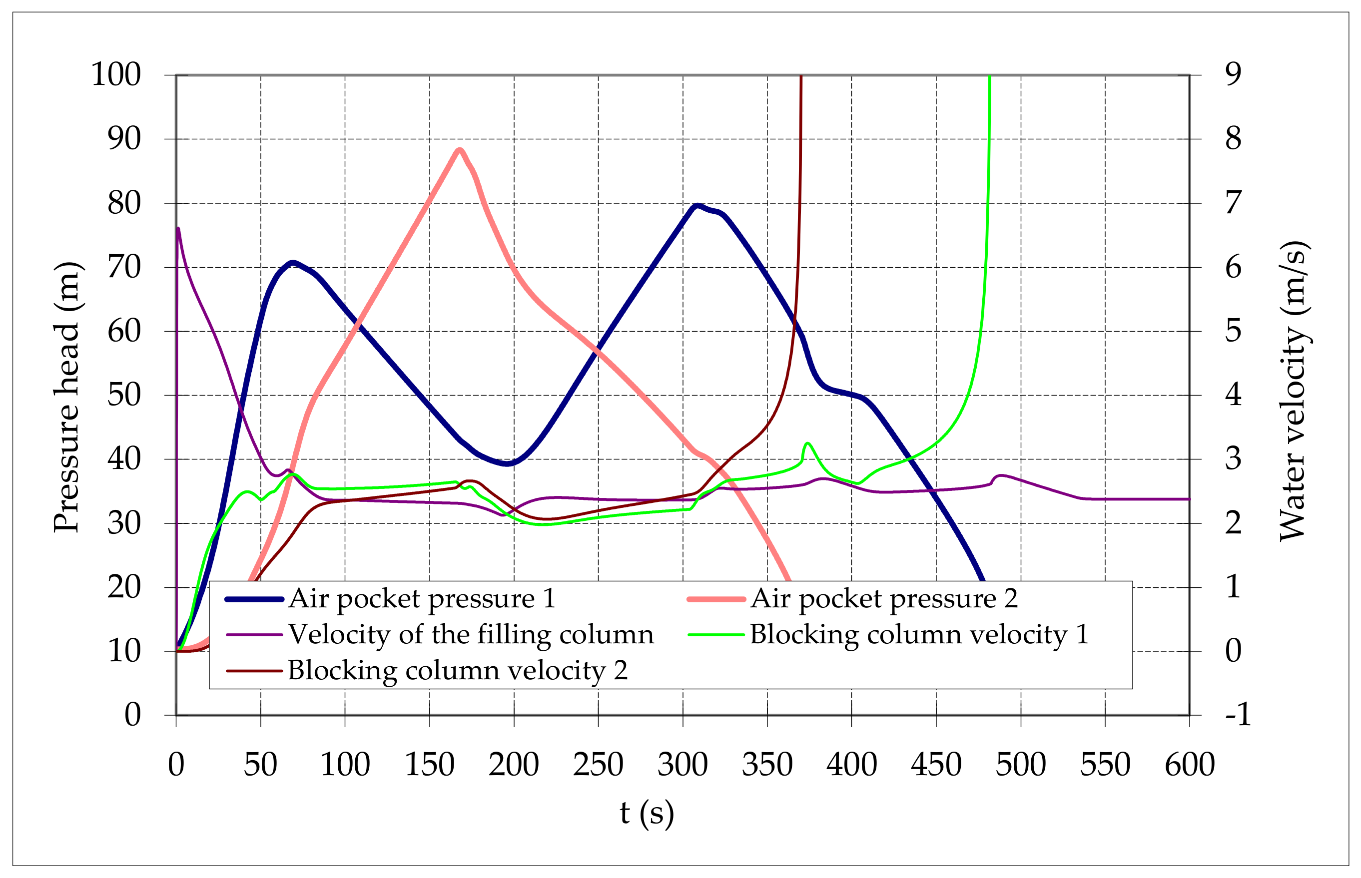
4.1. Numerical Resolution Using the Physical Equations

Employing the physical formulations developed by the authors (see Equations (30)–(36)), results concerning air-pocket pressure, filling-column velocity, and blocking-column velocity 1 were obtained, as shown in Figure 7.

Based on the results, the steady-state condition is reached at $t=$553.5 s. The filling column reaches the downstream reservoir at 33.2 s, while the blocking columns 1 and 2 reach this reservoir at 82.4 and 370.4 s, respectively.

Table 4. A summary of the results of the transient event using the physical equations.

Variable	Value	Time
Air-pocket pressure 1	$H_{1,max}^{\mathrm{*}}=70.70 \mathrm{m}$	$t=69.1 \mathrm{s}$
Air-pocket pressure 2	$H_{2,max}^{\mathrm{*}}=88.33 \mathrm{m}$	$t=167.8 \mathrm{s}$
Maximum velocity of the filling column	$v_{max}=6.613 \mathrm{m}/\mathrm{s}$	$t=1.1 \mathrm{s}$
Maximum velocity of blocking column 1	$v_{1,max}=2.767 \mathrm{m}/\mathrm{s}$	$t=69.1 \mathrm{s}$

summarises the main results of the analysed installation.

4.2. Results Employing the Proposed Methodology

This section presents the appication of charts developed in Section 3.2. In this case, a slow air-pocket pressure peak is obtained, since ${\mathsf{\Pi }}_m={\displaystyle \frac{H_e^{\mathrm{*}}}{H_{atm}^{\mathrm{*}}}}={\displaystyle \frac{5+10.33}{10.33}}=1.48$. Considering the chart for slow air-pocket pressure peaks (see Figure 4), then the relationship between $H_{max,1}^{\mathrm{*}}/H_e^{\mathrm{*}}$ is computed. After that, values of $H_{max}^{\mathrm{*}}$ can be computed using this relationship.

Table 5. Air-pocket pressure peaks computed using the proposed methodology.

Air Pocket	Dimensionless Parameters	${\mathit{H}}_{\mathit{m}\mathit{a}\mathit{x}}^{\mathbf{*}}/{\mathit{H}}_{\mathit{e}}^{\mathbf{*}}$	${\mathit{H}}_{\mathit{m}\mathit{a}\mathit{x}}^{\mathbf{*}}$ (m)
1	${\delta }_p={\displaystyle \frac{L_p sen{\theta }_p}{H_e^{\mathrm{*}}}}={\displaystyle \frac{155 \mathrm{m}-80 \mathrm{m}}{15.33 \mathrm{m}}}=4.89$	4.9	75.0
	${\alpha }_1={\displaystyle \frac{L_{b.1}}{L_{air\mathrm{1,0}}}}={\displaystyle \frac{280 \mathrm{m}}{198 \mathrm{m}}}=1.41$
2	${\delta }_p={\displaystyle \frac{L_p sen{\theta }_p}{H_e^{\mathrm{*}}}}={\displaystyle \frac{110 \mathrm{m}-50 \mathrm{m}}{15.33 \mathrm{m}}}=3.91$	5.5	84.0
	${\alpha }_1={\displaystyle \frac{L_{b.2}}{L_{air\mathrm{2,0}}}}={\displaystyle \frac{825 \mathrm{m}}{125 \mathrm{m}}}=6.6$

presents the calculations conducted in this scenario.

5. Discussion

5.1. Comparision

The results obtained using the proposed methodology are compared to those calculated using the physical equations (Section 4.1), as shown in

Table 6. A comparison between the proposed methodology and the physical equations.

Air Pocket	${\mathit{H}}_{\mathit{m}\mathit{a}\mathit{x}}^{\mathbf{*}}$ (m)		Discrepancy (%)
	Proposed Methodology	Physical Equations
1	75.0	70.7	6.08
2	84.0	88.3	4.90

. A discrepancy lower than 6.08% was obtained for the maximum air-pocket pressure, showing that the proposed methodology is suitable for making calculations. In this sense, the proposed methodology can be employed by water utilities to compute extreme air-pocket pressure peaks during filling operations.

5.2. Classification of Pressure Peaks

The boundary between fast and slow pressure peaks cannot be precisely defined in real water networks. An intermediate situation involving pressure surges cannot be defined with precision [10]. However, the most important aspect is the calculation of fast peaks, as this is where the highest pressure surges occur, which the installation must withstand.

Nevertheless, solving the complete model shows that significantly fewer factors contribute to the final value of the studied pressure peak. To this end, the fundamental criterion is the speed of the transient that generates it, which makes it necessary to group them into three categories: (i) fast pressure peaks, which are only possible in the first air pocket ($i=1$), which can be generated by transient events of a short duration and require significant energy sources (${\mathsf{\Pi }}_m\ge 5$) that, acting abruptly due to the instantaneous opening of the valve, must overcome small initial inertias (${\beta }_0\to 0$); (ii) slow pressure peaks, which are generated after the compression of an air pocket over minutes, which are characteristic of pockets far from the energy source (2$i\ge 2$), although they may also occur in the first air pocket if the parameter ${\mathsf{\Pi }}_m$ is small or ${\beta }_0$ is large (significant initial inertia); and (iii) moderate pressure peaks, whose final value is significantly influenced by the source of energy (${\mathsf{\Pi }}_m, \mu$) and the gravitational effects induced by the profile (${\delta }_p$).

6. Conclusions

The dimensionless treatment of the 3$n$ + 2 equations modelling the behaviour of $n$ entrapped air pockets within a pipeline with an irregular profile shows the dependence of an essential number of dimensionless parameters. To withdraw irrelevant parameters while maintaining the relevant ones, two types of pressure peaks, classified as fast and slow, have been considered. Fast peaks occur within seconds and slow peaks within minutes. The following conclusions can be drawn:

(a)

Fast peaks, which occur at the first air pocket when ${\mathsf{\Pi }}_m\ge 5$ and ${\beta }_0\to 0$ are characterised by the system parameter ${\alpha }_1={\beta }_1$ and two boundary parameters ${\mathsf{\Pi }}_m$ and $\mu$. Geometric contribution can safely be ignored.

(b)

Slow peaks are typical of second-to-last air pockets. Slow peaks are mainly influenced by gravitational forces, which must be considered through the single parameter ${\delta }_p$ corresponding to the reach where the air pocket under study is descending. This parameter, together with parameter ${ \alpha }_i$, allow for the estimation of slow peaks.

The present dimensionless analysis helps us to gain insight into the physics of the problem, giving more accurate knowledge of the most relevant factors. These, independently of the transient velocity, are:

(a)

The intensity and characteristics of the source(s) of energy, ${\mathsf{\Pi }}_m$, $\mu$, and ${\delta }_p$.

(b)

Parameter ${\alpha }_i$, i.e., the air-pocket capacity to store energy related to the inertia of its blocking column.

The charts corresponding to fast peaks are highly accurate, since the simplifications performed are justifiable. This is not the case for slow peaks, since after simplifying the geometric influence to a single parameter and neglecting friction and inertia, their chart, despite giving values within the same order of magnitude, can contain essential errors.

The proposed methodology offers reliability for computing rapid pressure peaks (through the developed charts), which are of utmost importance, as water utilities can use this methodology without solving the complex system of differential–algebraic equations. The proposed methodology provides a very close estimation of pressure surges for rapid events. For practical applications, the analysis of rapid pressure peaks is more critical compared to slow pressure surges.

The results of this study can be utilised by water utilities to address the challenges of filling operations, ensuring that the resulting pressure peaks remain within safe limits. These peaks can then be compared to a pipe’s resistance class to prevent pipeline ruptures.

References

1. Liou, C.P.; Hunt, W.A. Filling of Pipelines with Undulating Elevation Profiles. J. Hydraul. Eng. 1996, 122, 534–539. [Google Scholar] [CrossRef]
2. Wang, L.; Wang, F.; Karney, B.; Malekpour, A. Numerical Investigation of Rapid Filling in Bypass Pipelines. J. Hydraul. Res. 2017, 55, 647–656. [Google Scholar] [CrossRef]
3. Ferreira, J.P.; Ferràs, D.; Covas, D.I.C.; van der Werf, J.A.; Kapelan, Z. Air Entrapment Modelling during Pipe Filling Based on SWMM. J. Hydraul. Res. 2024, 62, 39–57. [Google Scholar] [CrossRef]
4. Fuertes-Miquel, V.S.; Coronado-Hernández, O.E.; Mora-Meliá, D.; Iglesias-Rey, P.L. Hydraulic Modeling during Filling and Emptying Processes in Pressurized Pipelines: A Literature Review. Urban Water J. 2019, 16, 299–311. [Google Scholar] [CrossRef]
5. Izquierdo, J.; Fuertes, V.S.; Cabrera, E.; Iglesias, P.L.; Garcia-Serra, J. Pipeline Start-up with Entrapped Air. J. Hydraul. Res. 1999, 37, 579–590. [Google Scholar] [CrossRef]
6. Zhou, L.; Liu, D.; Karney, B. Investigation of Hydraulic Transients of Two Entrapped Air Pockets in a Water Pipeline. J. Hydraul. Eng. 2013, 139, 949–959. [Google Scholar] [CrossRef]
7. Ramezani, L.; Karney, B.; Malekpour, A. Encouraging Effective Air Management in Water Pipelines: A Critical Review. J. Water Resour. Plan Manag 2016, 142, 4016055. [Google Scholar] [CrossRef]
8. Ramezani, L.; Karney, B.; Malekpour, A. The Challenge of Air Valves: A Selective Critical Literature Review. J. Water Resour. Plan Manag. 2015, 141, 4015017. [Google Scholar] [CrossRef]
9. American Water Works Association (AWWA). Air-Release, Air/Vacuum, and Combination Air Valves: M51; American Water Works Association: Denver, CO, USA, 2001; Volume 51. [Google Scholar]
10. Abreu, J.; Cabrera, E.; Izquierdo, J.; García-Serra, J. Flow Modeling in Pressurized Systems Revisited. J. Hydraul. Eng. 1999, 125, 1154–1169. [Google Scholar] [CrossRef]
11. Fuertes-Miquel, V.S.; López-Jiménez, P.A.; Martínez-Solano, F.J.; López-Patiño, G. Numerical Modelling of Pipelines with Air Pockets and Air Valves. Can. J. Civ. Eng. 2016, 43, 1052–1061. [Google Scholar] [CrossRef]
12. Martin, C.S. Entrapped Air in Pipelines. In Proceedings of the 2nd International Conference on Pressure Surges, London UK, 22–24 September 1976; British Hydromechanics Research Assoc.: Cranfield, UK, 1976. [Google Scholar]
13. Tullis, J.; Watkins, R. Pipe Collapse Caused by a Pipe Rupture—A Case Study. In Hydraulic Transients with Water Column Separation; 9th and Last Round Table of the IAHR Group: Valencia, Spain, 1991. [Google Scholar]
14. de Almeida, A.B.; Koelle, E. Fluid Transients in Pipe Networks; Computational Mechanics Publications; Springer: Berlin/Heidelberg, Germany, 1992. [Google Scholar]
15. Zhou, L.; Liu, D.; Karney, B.; Zhang, Q. Influence of Entrapped Air Pockets on Hydraulic Transients in Water Pipelines. J. Hydraul. Eng. 2011, 137, 1686–1692. [Google Scholar] [CrossRef]
16. Coronado-Hernández, Ó.E.; Besharat, M.; Fuertes-Miquel, V.S.; Ramos, H.M. Effect of a Commercial Air Valve on the Rapid Filling of a Single Pipeline: A Numerical and Experimental Analysis. Water 2019, 11, 1814. [Google Scholar] [CrossRef]
17. Zhou, L.; Pan, T.; Wang, H.; Liu, D.; Wang, P. Rapid Air Expulsion through an Orifice in a Vertical Water Pipe. J. Hydraul. Res. 2019, 57, 307–317. [Google Scholar] [CrossRef]
18. Fang, H.; Zhou, L.; Cao, Y.; Cai, F.; Liu, D. 3D CFD Simulations of Air-Water Interaction in T-Junction Pipes of Urban Stormwater Drainage System. Urban Water J. 2022, 19, 74–86. [Google Scholar] [CrossRef]
19. He, J.; Hou, Q.; Lian, J.; Tijsseling, A.S.; Bozkus, Z.; Laanearu, J.; Lin, L. Three-Dimensional CFD Analysis of Liquid Slug Acceleration and Impact in a Voided Pipeline with End Orifice. Eng. Appl. Comput. Fluid Mech. 2022, 16, 1444–1463. [Google Scholar] [CrossRef]
20. Martins, N.M.C.; Delgado, J.N.; Ramos, H.M.; Covas, D.I.C. Maximum Transient Pressures in a Rapidly Filling Pipeline with Entrapped Air Using a CFD Model. J. Hydraul. Res. 2017, 55, 506–519. [Google Scholar] [CrossRef]
21. Memon, Q.A.; Al Ahmad, M.; Pecht, M. Quantum Computing: Navigating the Future of Computation, Challenges, and Technological Breakthroughs. Quantum Rep. 2024, 6, 627–663. [Google Scholar] [CrossRef]
22. Zhou, L.; Lu, Y.; Karney, B.; Wu, G.; Elong, A.; Huang, K. Energy Dissipation in a Rapid Filling Vertical Pipe with Trapped Air. J. Hydraul. Res. 2023, 61, 120–132. [Google Scholar] [CrossRef]
23. Malekpour, A.; Shahroodi, A. What Is a Safe Filling Velocity in Water and Wastewater Pipelines? In Pipelines 2023; ASCE: Reston, VA, USA, 2023; pp. 301–312. [Google Scholar] [CrossRef]
24. Fuertes-Miquel, V.S. Hydraulic Transients with Entrapped Air Pockets. Ph.D. Thesis, Polytechnic University of Valencia, Spain, Valencia, 2001. [Google Scholar]
25. Fuertes-Miquel, V.S.; Coronado-Hernández, O.E.; Arrieta-Pastrana, A. Effects of Expelled Air during Filling Operations with Blocking Columns in Water Pipelines of Undulating Profiles. Fluids 2024, 9, 212. [Google Scholar] [CrossRef]
Figure 1. The pipeline scheme for a filling procedure.
Mathematics 13 00267 g001
Figure 2. Methodology used in this study.
Mathematics 13 00267 g002
Figure 3. Charts for fast peaks with n = 1.2 and β 0 0 for: (a) Π m = 5 ; (b) Π m = 10 ; (c) Π m = 20 ; and (d) Π m = 30 .
Mathematics 13 00267 g003
Figure 4. Chart for slow peaks with n = 1.2 and β 0 0 .
Mathematics 13 00267 g004
Figure 5. The boundary between fast and slow air-pocket pressure peaks.
Mathematics 13 00267 g005
Figure 6. The characteristics of the analysed water installation.
Mathematics 13 00267 g006
Figure 7. An analysis of the transient flow employing the physical equations.
Mathematics 13 00267 g007