A Consensus Community-Based Spider Wasp Optimization for Dynamic Community Detection

Abstract

There are many evolving dynamic networks in the real world, and community detection in dynamic networks is crucial in many complex network analysis applications. In this paper, a consensus community-based discrete spider wasp optimization (SWO) approach is proposed for the dynamic network community detection problem. First, the coding, initialization, and updating strategies of the spider wasp optimization algorithm are discretized to adapt to the community detection problem. Second, the concept of intra-population and inter-population consensus community is proposed. Consensus community is the knowledge formed by the swarm summarizing the current state as well as the past history. By maintaining certain inter-population consensus community during the evolutionary process, the population in the current time window can evolve in a similar direction to those in the previous time step. Experimental results on many artificial and real dynamic networks show that the proposed method produces more accurate and robust results than current methods.

1. Introduction

Over time, the discovery of community structure in complex networks has become a key task for researchers engaged in network analysis. The concept of community is most directly recognized as a set of clusters with tight internal connections and sparse external connections [1]. A community can be understood as a class of people, objects, or events with similar attributes, the same function, and consistent characteristics [2]. Examples include friends with the same hobby in a social network, proteins with the same function in a biological protein network, bottlenose dolphins affiliated with the same organization, and so on. The essential work of community structure detection is to discover members belonging to the same community from a complex interwoven network. Community detection, as an effective technique to reveal underlying structures, has been applied in many scenarios, such as social relationship analysis [3], recommendation systems [4], link prediction [5,6], and virus transmission [7,8].

Early researchers regarded the community detection problem as a clustering problem and used traditional clustering methods to divide communities. Newman proposed a modularity function to assess the quality of the structure of the divided communities from a methodological point of view, transforming the community detection problem from a traditional clustering problem to an optimization problem. As an objective function in optimization methods, the modularity function suffers from resolution limitations [9], as well as weighted directed network applicability problems [10]. Therefore, many new community structure quality assessment functions have been proposed, such as modularity density function [11], weighted directed network modularity function [12], overlapping community modularity function [13], etc. Based on the above evaluation functions, many excellent research works such as GA-Net [14], Meme-Net [15], MOGA-Net [16], MOPSO-Net [17], and so on have emerged. These algorithms better serve static network community detection; however, many networks originated from the real world are overwhelmingly dynamic, and the problem of dynamic network community detection has attracted more researchers’ attention.

Community detection in dynamic networks is performed independently for each snapshot network, supplemented by a static algorithm for detection. Palla et al. [18] applied a faction filtering algorithm to a dynamic network, and then matched communities at neighboring time points. However, the method does not consider the community structure connection between snapshot networks, and the community division and community evolution are separated, which cannot reflect the nature of community dynamic evolution. Sun et al. [19] divided the network into a series of snapshots and proposed a lightweight evolutionary event detection algorithm to discover the community evolution events between neighboring snapshots. The parallelization of the algorithm is achieved by dividing the snapshot network community relatively independently. However, since the snapshot networks are too independent, the community structure with valuable information in the historical snapshot network is ignored, resulting in the need to reclassify the community structure of the whole snapshot network even when the network undergoes minor changes. Folina and Pizzuti proposed a multi-objective genetic algorithm named DYNMOGA based on an evolutionary clustering framework [20]. By optimizing two objective functions, modularity and normalized mutual information, the DYNMOGA algorithm was able to achieve community detection in dynamic networks but with high time complexity.

Most of the existing methodological frameworks for solving the dynamic network community detection problem are narrated as multi-objective optimization and evolutionary algorithms in reference [21]. However, there is a serious problem with methods based on multi-objective optimization. The simultaneous optimization of two objective functions can indeed achieve a balance of objectives in both directions. However, since the dominated solution determines the direction of evolution, many solution schemes may be extremely optimal in one objective and extremely poor in the other, and such solutions will be retained because they cannot be dominated. The algorithm will consume more individuals and more time to explore the best solution.

To address the above problems, the concept of consensus community is introduced in this paper. Identify similar community between the current population and the optimal population in the previous generation of individuals. By keeping these similarity communities constant during evolution, it ensures that individuals are guided by consensus community to move to similar community structure in the previous generation during each evolutionary process. The main contributions of this paper can be summarized as follows:

(1)

The concept of consensus communities is introduced. By mining consensus community from the previous generation, a certain continuity of the iterations between populations is maintained. This is used to optimize the time and space loss required for evolution.

(2)

The spider wasp optimization algorithm is discretized. The coding method and the position update strategy for discrete scenes are improved. A key node-based initialization strategy is designed to improve the quality of initial individuals.

(3)

A framework of consensus swarm-based spider wasp optimization algorithm is designed for detecting swarm structures in dynamic complex networks. Since the number of communities is determined by the decoding of the representation, the SWO-Net algorithm does not need to specify the number of communities and weight parameters for recognizing the network.

(4)

Experiments on synthetic and real datasets validate the effectiveness of the SWO-Net algorithm. Comparison experiments with other benchmark algorithms show that the SWO-Net algorithm has significant advantages.

The rest of the paper is organized as follows. Section 2 briefly introduces the multi-objective approach for community detection in static and dynamic networks; Section 3 introduces the concept and principle of consensus community; Section 4 demonstrates the constructed SWO-Net multi-objective community detection algorithm for dynamic networks in detail; and Section 5 conducts comparative experiments from multiple perspectives to validate the validity and sophistication of the proposed algorithm.

2. Background and Related Works

2.1. Dynamic Community Detection

A dynamic network can be described as a sequence $G=\left\{G_1,G_2,\cdots ,G_T\right\}$, where $G_i$ denotes a network snapshot of the connectivity relationship between nodes at time i. The number of nodes in the network and the connectivity between nodes varies at each moment in time. Nodes and connectivity relationships in a dynamic network change over time. Some nodes drop out of the network, and their associated edges disappear from the network. Some nodes are added to the network, thus creating connectivity relationships with the original nodes in the network. The dynamic network changes from time $T_i$ to time $T_{i+1}$ are given in Figure 1, where node 2 exits the network and edges $e_{1,2}$ and $e_{2,3}$ disappear; node 11 joins the network and produces three new edges, $e_{1,11}$, $e_{3,11}$ and $e_{5,11}$.

Chakrabarti et al. [22] proposed the concept of evolutionary clustering, which produces a series of clusters by introducing a temporal smoothing framework to group data at different time steps. Evolutionary clustering assumes that the community structure does not change suddenly and drastically over a short period of time, thus smoothing the community structure of the network at each time step over time. Smoothing is achieved by making a trade-off between two different goals, the first goal is known as snapshot quality, which means that the results of the clustering should reflect the community structure of the network at the current time step as much as possible. The second goal is referred to as time cost, meaning that each clustering result refuses to produce drastic changes from one time step to another.

Kherad [23] proposed a dynamic network community detection algorithm that can address both key node identification and overlapping communities. It outperforms the existing state-of-the-art methods in terms of modularity and computational complexity. Ranjkesh [24] proposed a robust modeling algorithm for dynamic community structure detection for attacks in complex networks. The method does not need to determine the number of communities and is able to detect communities with high accuracy and stability. Zhou [25] proposed an attribute-based Node2Vec method to generate node embeddings, complemented by a modularity-based community detection method for community identification.

2.2. The SWO Algorithm

Mohamed et al. [26] proposed a new nature-inspired meta-heuristic-based algorithm, the spider wasp optimization (SWO) algorithm, in 2023, which is inspired by the hunting, nesting, and mating behaviors of female spider wasps in nature, and has a variety of unique updating strategies for a variety of NP-hard problems. The spider wasp algorithm simulates the biological behavior of spider wasps and can be summarized in four parts:

(1)

Search behavior.

The search behavior drives the algorithm to seek out prey at the start of optimization, looking for spiders that are suitable for larval growth. Female spider wasps explore the hunting space randomly with a constant step size, a behavior that can be mathematically modeled as

$${\overrightarrow{S{W}_i}}^{t+1}={\overrightarrow{S{W}_i}}^t+{\mu }_1\times \left({\overrightarrow{S{W}_a}}^t-{\overrightarrow{S{W}_b}}^t\right)$$

(1)

$${\mu }_1=\left|rn\right|\times r_1$$

(2)

where a and b are two random individuals in the population; ${\mu }_1$ denotes a definite step size; $r_1$ is a random number between 0 and 1; and $\left|rn\right|$ is a random number that conforms to a normal distribution. Female wasps may sometimes fail to find a spider that has fallen from a spider web, so the algorithm allows female wasps to search the area near the spider’s fall point, and the mathematical expression for this search behavior is

$$\left\{\begin{array}{c}{\overrightarrow{SW}}_i^{t+1}={\overrightarrow{SW}}_c^t+{\mu }_2\times \left(\overrightarrow{L}+\overrightarrow{r_2}\times \left(\overrightarrow{H}-\overrightarrow{L}\right)\right)\hfill \\ {\mu }_2=B\times cos\left(2\pi l\right)\hfill \\ B={\displaystyle \frac{1}{1+e^l}}\hfill \end{array}\right.$$

(3)

where c denotes a randomly selected female wasp in the population; l is a random number between −2 and 1. By randomizing both Equations (1) and (3) searches, the female wasp moves towards the possible location of the spider. $r_3$ and $r_4$ are a pair of random numbers:

$${\overrightarrow{SW}}_i^{t+1}=\left\{\begin{array}{c}Equation\left(1\right)r_3<r_4\hfill \\ Equation\left(3\right)otherwise\hfill \end{array}\right.$$

(4)

(2)

Following and escaping behavior.

After spotting their prey/spiders, they may try to escape. Therefore, female spider wasps follow their prey, paralyzing and dragging the fittest one. This behavior simulates two possible trends: the first is that the female wasp traps the spider, and in this scenario, Equation (5) is applied to update the position of the female wasp. C denotes the control factor for the speed of female bees, which decays from 2 to 0. When $C<0.5$, the spider is faster than the female wasp, and the distance between them gradually increases; when $C>0.5$, the female wasp is faster than the spider, and the distance between them gradually decreases:

$$\left\{\begin{array}{c}{\overrightarrow{SW}}_i^{t+1}={\overrightarrow{SW}}_i^t+C\times \left|2\times \overrightarrow{r_5}\times {\overrightarrow{SW}}_a^t-{\overrightarrow{SW}}_i^t\right|\hfill \\ C=\left(2-2\times \left({\displaystyle \frac{t}{t_{max}}}\right)\right)\times r_6\hfill \end{array}\right.$$

(5)

where a is a randomly selected individual from the population; t and $t_{max}$ denote the current iteration number and the maximum iteration number, respectively; $\overrightarrow{r_5}$ is a random vector in the interval [0,1]; and $r_6$ denotes a random number in the interval [0,1]. The second possible trend is that by simulating the spider escaping from the female wasp pursuit, the distance between the female wasp and the spider gradually increases; this phase is the initial exploitation phase. As the distance increases, the exploitation phase shifts to the exploration phase, in which case Equation (6) is applied to update the position of the female wasp. It is simulated in the following mathematical form:

$$\left\{\begin{array}{c}{\overrightarrow{SW}}_i^{t+1}={\overrightarrow{SW}}_i^t\times \overrightarrow{vc}\hfill \\ k=1-\left({\displaystyle \frac{t}{t_{max}}}\right)\hfill \end{array}\right.$$

(6)

where $\overrightarrow{vc}$ is a vector between k and $-k$ according to the normal distribution. The trade-off between the above two trends is realized stochastically by Equation (7):

$${\overrightarrow{SW}}_i^{t+1}=\left\{\begin{array}{c}Equation\left(5\right)r_3<r_4\hfill \\ Equation\left(6\right)otherwise\hfill \end{array}\right.$$

(7)

In order to search globally, the authors use the follow-and-avoid mechanism for optimization in the expectation of discovering the optimal solution region and avoiding falling into the local minima, and adjust the search and follow mechanism by the following formula:

$${\overrightarrow{SW}}_i^{t+1}=\left\{\begin{array}{c}Equation\left(4\right)p<k\hfill \\ Equation\left(7\right)otherwise\hfill \end{array}\right.$$

(8)

(3)

Nesting behavior.

The process is based on two equations that simulate dragging prey to the vicinity of a nest of suitable prey and egg size. The first equation is a simulation of pulling a spider towards the best place suitable for constructing a nest in order to prevent paralyzed spider from escaping and laying eggs on the spider’s abdomen. The first equation is described mathematically as follows:

$${\overrightarrow{SW}}_i^{t+1}={\overrightarrow{SW}}^{*}+cos\left(2\pi l\right)\times \left({\overrightarrow{SW}}^{*}-{\overrightarrow{SW}}_i^t\right)$$

(9)

where ${\overrightarrow{SW}}^{*}$ denotes the best solution at the current stage. The second equation will randomly select female wasp from the population and nest at their location, avoiding multiple nesting at the same location by an additional step size:

$${\overrightarrow{SW}}_i^{t+1}={\overrightarrow{SW}}_a^t+r_3\times \left|\gamma \right|\times \left({\overrightarrow{SW}}_a^t-{\overrightarrow{SW}}_i^t\right)+\left(1-r_3\right)\times \overrightarrow{U}\left({\overrightarrow{SW}}_a^t-{\overrightarrow{SW}}_c^t\right)$$

(10)

where $\gamma$ is a value generated from lévy flight; a, b, and c are three individual female bees randomly selected from the population; U is a binary vector used to determine when a step is used to avoid nesting multiple times at the same location; and U is assigned the following formula:

$$\overrightarrow{U}=\left\{\begin{array}{c}1\overrightarrow{r_4}>\overrightarrow{r_5}\hfill \\ 0otherwise\hfill \end{array}\right.$$

(11)

The two processes are randomly switched by the following equation:

$${\overrightarrow{SW}}_i^{t+1}=\left\{\begin{array}{c}Equation\left(9\right)r_3<r_4\hfill \\ Equation\left(10\right)otherwise\hfill \end{array}\right.$$

(12)

Finally, the switch between hunting and nesting behavior is made via Equation (13). All female wasps will search for the corresponding spiders at the beginning of the optimization process and pull them to a suitable location for nesting:

$${\overrightarrow{SW}}_i^{t+1}=\left\{\begin{array}{c}Equation\left(8\right)i<N\times k\hfill \\ Equation\left(12\right)otherwise\hfill \end{array}\right.$$

(13)

(4)

Mating behavior.

The simulation produces hatched eggs by using the same uniform crossover operation between male spider wasps $S_m^t$ and female spider wasps $S_i^t$, where males generate locations through females:

$$S{W}_i^{t+1}=Crossover(S{W}_i^t,S{W}_m^t,CR)$$

(14)

$${\overrightarrow{SW}}_m^{t+1}={\overrightarrow{SW}}_i^t+e^l\left|\beta \right|\overrightarrow{v_1}+\left(1-e^l\right)\left|{\beta }_1\right|\overrightarrow{v_2}$$

(15)

The above equations $\beta$ and ${\beta }_1$ are two random numbers generated according to the normal distribution, e is an exponential constant, and the vectors $\overrightarrow{v_1}$ and $\overrightarrow{v_2}$ are generated by the following equation:

$$\overrightarrow{v_1}=\left\{\begin{array}{c}\overrightarrow{x_a}-\overrightarrow{x_i}f\left(\overrightarrow{x_a}\right)<f\left(\overrightarrow{x_i}\right)\hfill \\ \overrightarrow{x_i}-\overrightarrow{x_a}otherwise\hfill \end{array}\right.$$

(16)

$$\overrightarrow{v_2}=\left\{\begin{array}{c}\overrightarrow{x_b}-\overrightarrow{x_c}f\left(\overrightarrow{x_b}\right)<f\left(\overrightarrow{x_c}\right)\hfill \\ \overrightarrow{x_c}-\overrightarrow{x_b}otherwise\hfill \end{array}\right.$$

(17)

When a female wasp closes the nest after completing egg laying, it means that the female will not continue to participate in subsequent optimizations. The simulation of this behavior allows the population size to be reduced, providing more opportunities for other females to optimize and speed up the approach to the optimal solution. At each evaluation of the whole function, the length of the new population will be updated by applying the following equation:

$$N=N_{min}+\left(N-N_{min}\right)\times k$$

(18)

where $N_{min}$ denotes the minimum number of populations set to avoid falling into local minima. The pseudo-code for the SWO is given in Algorithm 1.

Algorithm 1 Pseudo-code for the SWO algorithm.
begin
Input:  N, $N_{min}$, $CR$, $TR$, $t_{max}$
1:	Initialize the population $\overrightarrow{SW}=\left(\overrightarrow{S{W}_1},\overrightarrow{S{W}_2},\cdots ,\overrightarrow{S{W}_N}\right)$
2:	Calculate the fitness function to find the best solution ${\overrightarrow{SW}}^{*}$
3:	$t=1$
4:	while  $t<t_{max}$  do
5:	if $r_6<TR$ then
6:	for $i=1:N$ do
7:	Execute Equation (13) and calculate the fitness value
8:	$t=t+1$
9:	end for
10:	else
11:	for $i=1:N$ do
12:	Perform Equation (14) for uniform crossover
13:	$t=t+1$
14:	end for
15:	end if
16:	Reducing the population size through the Equation (18)
17:	end while
Output: the best solution ${\overrightarrow{SW}}^{*}$.

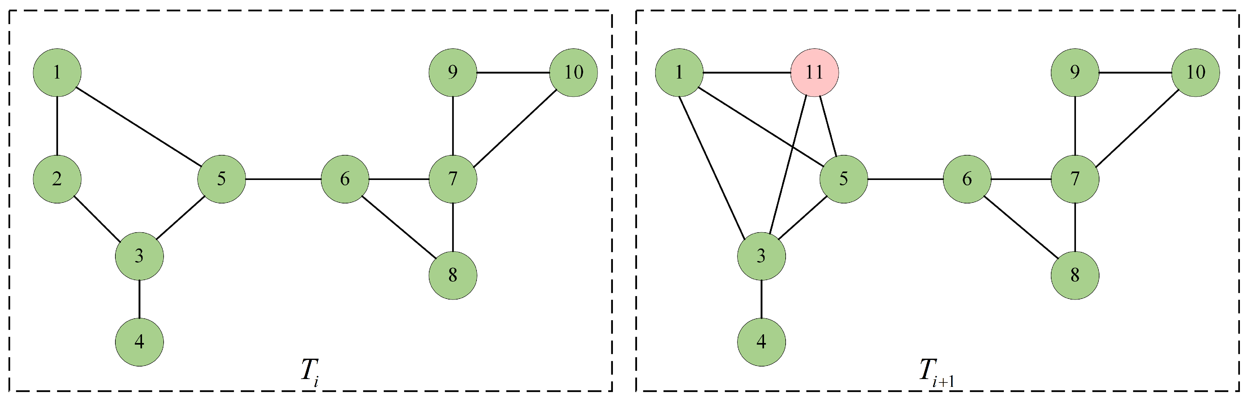
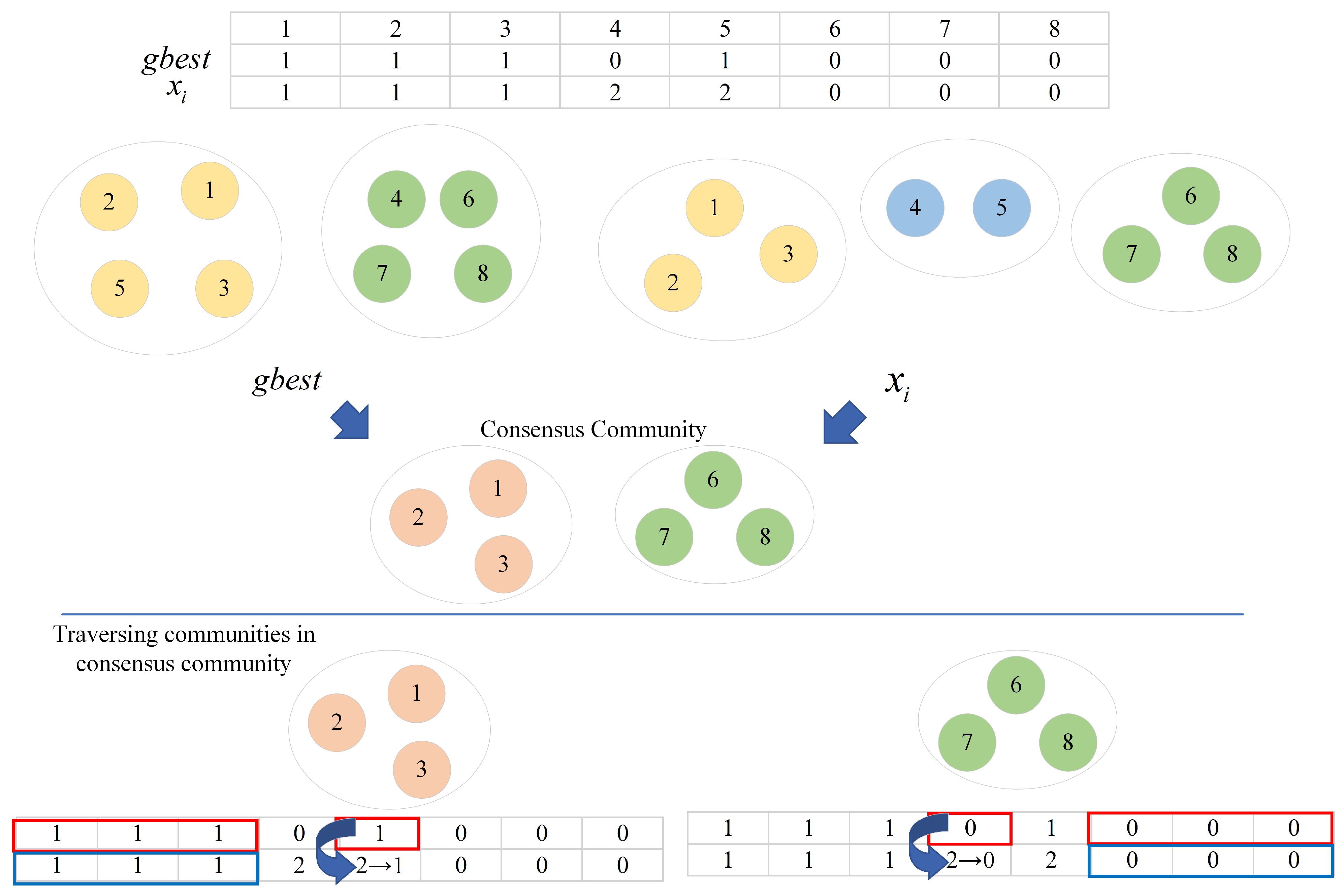
3. Consensus Community

The concept of consensus community has been mentioned in previous studies [27,28,29]. In [27], the concept of consensus clustering was proposed, where, after a community detection algorithm is run n times, it will obtain the community structures corresponding to its n results, and consensus clustering of the n community structures can obtain a consensus community with the highest similarity to the n results. In this section, two concepts of intra-population consensus community and inter-population consensus community are proposed for the dynamic community detection problem. The algorithm extracts the intra-population consensus community in the current iteration from multiple representative individuals in the population as the knowledge accumulated during the population iteration. A few communities with higher support in the intra-population consensus community are used as the inter-population consensus community to guide the next-generation group to move towards the optimal solution.

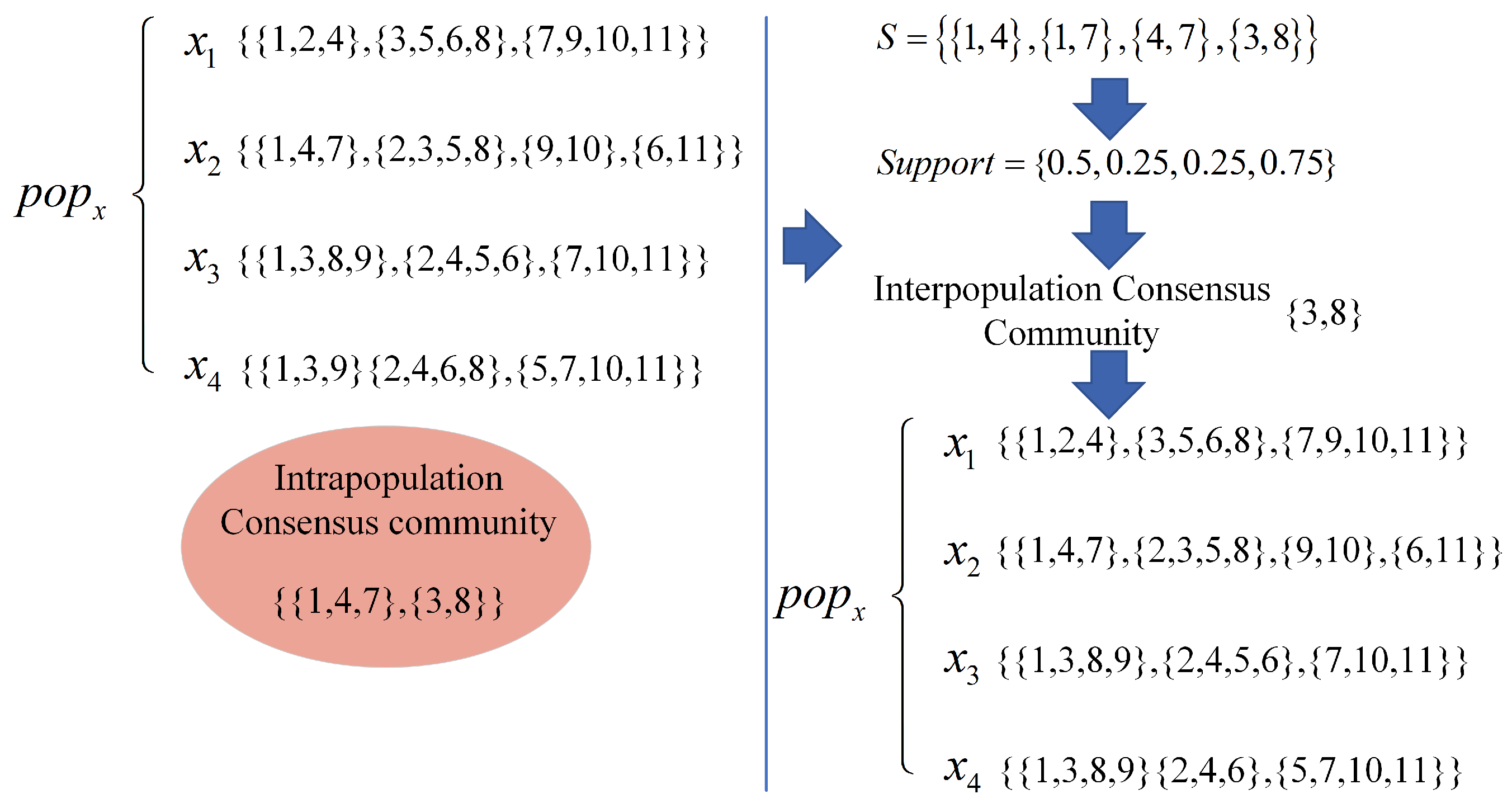
3.1. Intra-Population Consensus Community

The intra-population consensus community is obtained by jointly nudging multiple individuals that are most representative of the current iteration population. The best-performing individual under the $f_1$ objective function, and the best-performing individual under the $f_2$ objective function, as well as the knee solution $x^{*}$ [30], are chosen as the representative individuals for nudging the consensus community, respectively. The knee solution is similar to the global optimal solution in that both are a trade-off value under multiple objectives. The mathematical expression of the knee solution is given below:

$$x^{*}={arg}_x\underset{x\in PS}{min}\left({\displaystyle \frac{f_1\left(x\right)-min{f}_1}{max{f}_1-min{f}_1}}+{\displaystyle \frac{f_2\left(x\right)-min{f}_2}{max{f}_2-min{f}_2}}\right)$$

(19)

where $PS$ denotes the pareto optimal solution set. The intra-population consensus community is obtained by intersecting the community structures represented by the three individuals. Assuming that $C_1$, $C_2$, and $C_3$ denote the community structures represented by $min{f}_1$ individual, $min{f}_2$ individual, and $x^{*}$, respectively, the intra-population consensus community $\mathrm{int}r{a}_{CC}=\left(C_1,C_2,C_3\right)=\left\{c_{1i}\cap c_{2j}\cap c_{3k}\right\}$, where $c_{1i}\in C_1,c_{2j}\in C_2,c_{3k}\in C_3$, $\left\{c_{1i}\cap c_{2j}\cap c_{3k}\right\}$ denotes the number of common nodes within the intersection of the three communities, $|c_{1i}\cap c_{2j}\cap c_{3k}|\ge 2$. As shown in Figure 2, the community $C_1$ = $\left\{\left\{1,4,5,7\right\},\{3,8,11\},\{2,6,9\},\{10,11\}\right\}$ for individual $min{f}_1$. The community of individual $min{f}_2$ is $C_2$ = $\left\{\left\{1,4,7\right\},\{2,3,8,12\},\{6,10\},\{5,9,11\}\right\}$. The community $C_3$ for $x^{*}$ is $C_3$ = $\left\{\left\{1,4,5,7\right\},\left\{3,8,10\right\},\left\{2,9\right\},\left\{6,11\right\}\right\}$. Communities $\left|\left\{1,4,5,7\right\}\cap \left\{1,4,7\right\}\cap \left\{1,4,5,7\right\}\right|=3\ge 2$ in $C_1$, $C_2$, and $C_3$, so $\left\{1,4,7\right\}$ are added to the consensus community. $\left|\left\{1,4,5,7\right\}\cap \left\{6,11\right\}\right.$$\left.\cap \left\{2,3,8,12\right\}\right|=0<2$, and three consensus communities are not generated. Iterating through all communities, the final obtained consensus community is $\left\{\left\{1,4,7\right\},\left\{3,8\right\}\right\}$

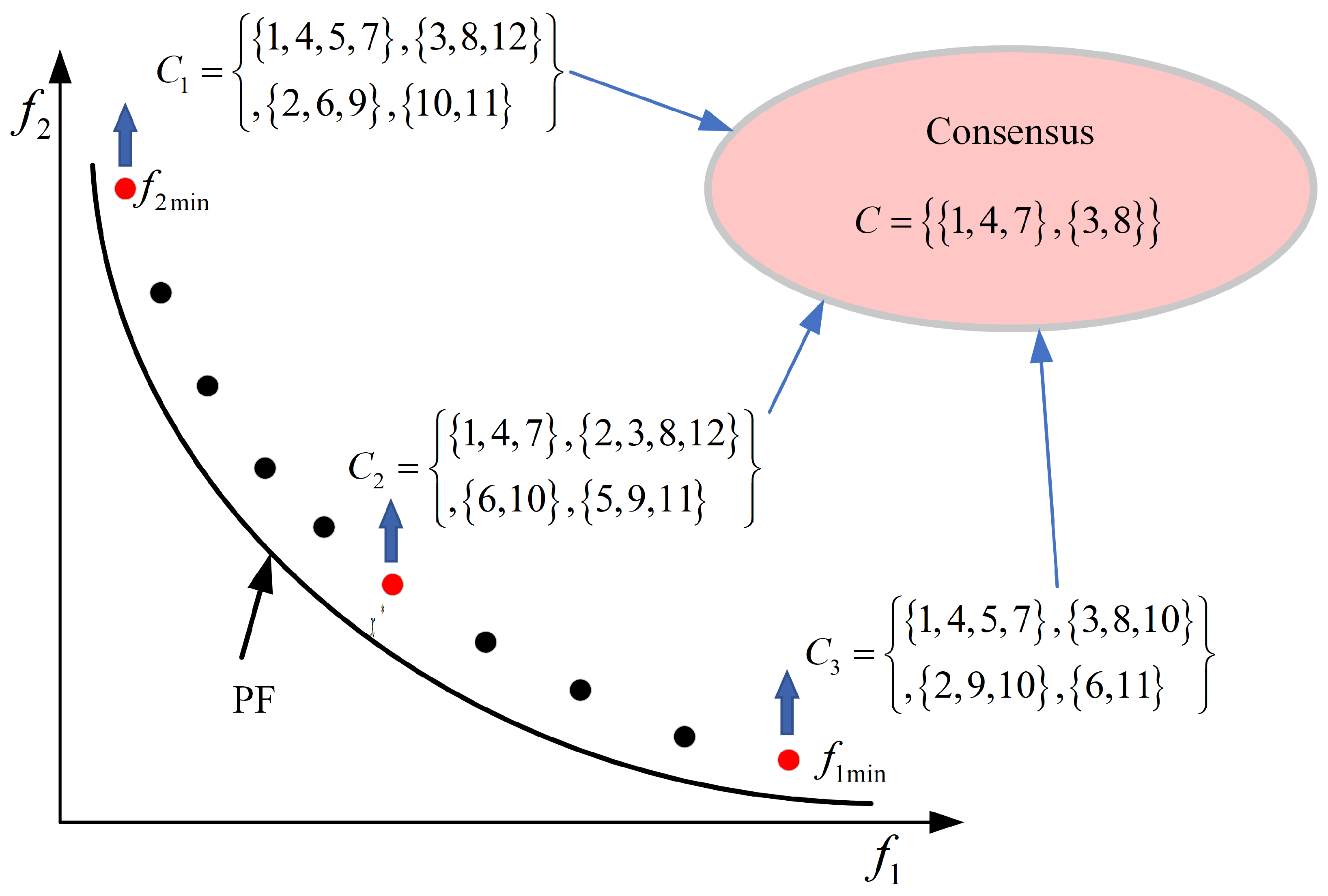
3.2. Inter-Population Consensus Community

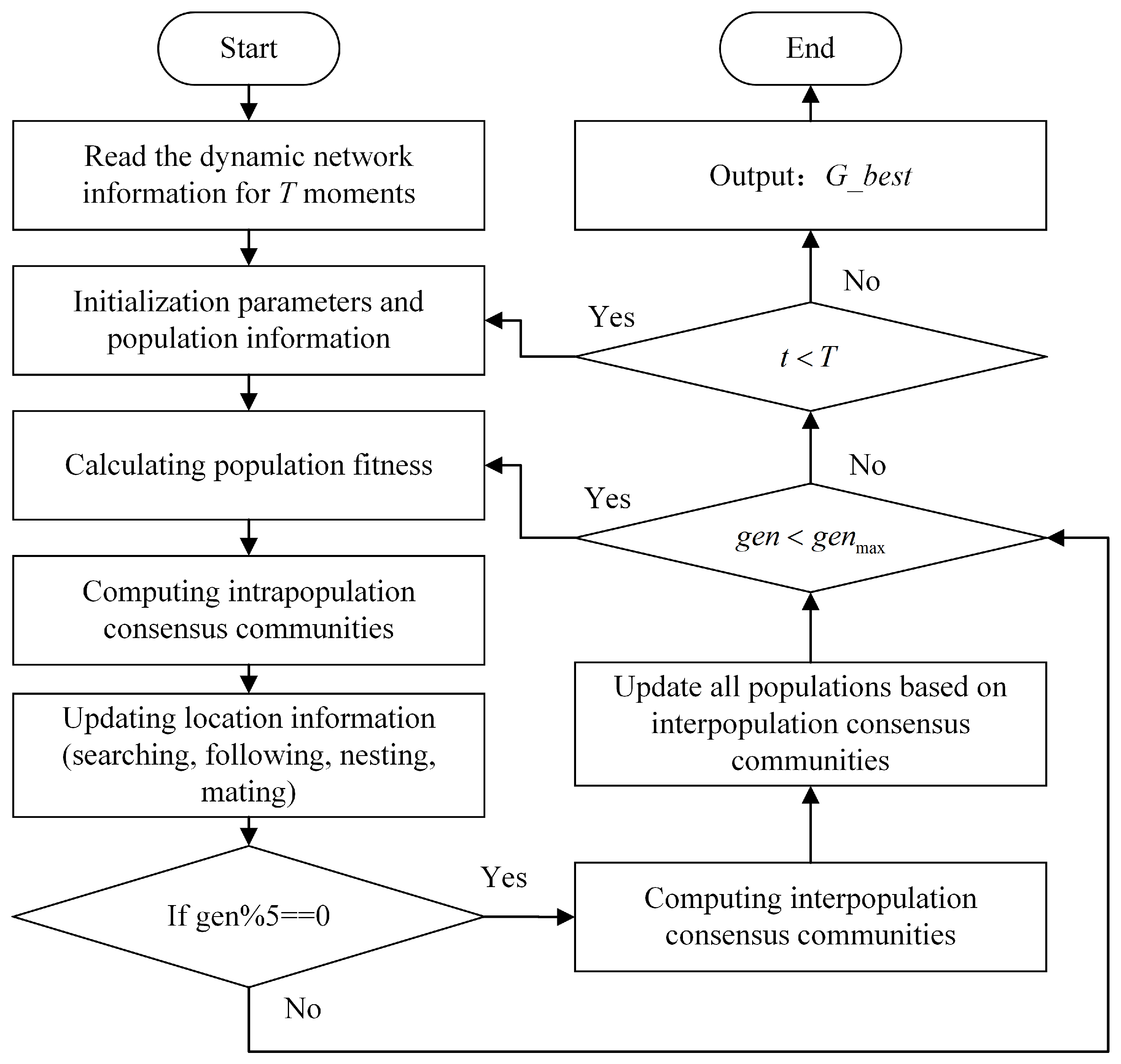
After obtaining the consensus community within the previous population as knowledge, support is used to assess the probability that a community may occur between populations. Assuming that the current population $po{p}_x=\left\{x_1,x_2,\cdots ,x_n\right\}$, $C_i=\left\{c_1,c_2,\cdots ,c_p\right\}$ denotes the solution of the ith individual divides the network into p communities. Given an intra-population consensus community $\mathrm{int}r{a}_{CC}=\left\{iac{c}_1,iac{c}_2,\cdots \right\}$, $S=\left\{s_1,s_2,\cdots \right\}$, where $s_i$ denotes the pair of nodes formed by the two-by-two combination of the nodes in $iac{c}_j$, the support of $po{p}_x$ for $s_i$ is denoted as

$$Support(s_i,po{p}_x)={\displaystyle \frac{\left|s_i\subset c_j,c_j\subset C_k,C_k\subset po{p}_x\right|}{\left|po{p}_x\right|}}$$

(20)

As shown in Figure 3, node pairs are constructed for the nodes in the in-population consensus community to form $S=\left\{\left\{1,4\right\},\left\{4,7\right\},\left\{1,7\right\},\left\{3,8\right\}\right\}$, with the population information $po{p}_x=\left\{x_1,x_2,x_3,x_4\right\}$. $s_1=\left\{1,4\right\}\subset x_1,x_2$, and hence the support of $po{p}_x$ for node pair $s_1$ is $\left|x_1,x_2\right|/\phantom{\left|x_1,x_2\right|\left|x_1,x_2,x_3,x_4\right|=0.5}\left|x_1,x_2,x_3,x_4\right|=0.5$. The support of all node pairs is compared with a preset support threshold of 0.75; node pairs greater than the threshold are added to the inter-population consensus community, and node pairs less than the threshold are ignored. In order to reduce the complexity of the algorithm, we choose to update the inter-population consensus community every five iterations on the population.

4. Proposed Method

In this section, the SWO algorithm is taken as the main framework, and the SWO-Net algorithm model applicable to the dynamic complex network community detection problem is formed by redefining the initialization strategy, location representation, and population update in the SWO algorithm, combined with the intra-population and inter-population consensus community strategy. The four behaviors in the SWO algorithm, search behavior, following and escaping behavior, nesting behavior, and mating behavior, are redesigned and discretized, while the intra-population and inter-population consensus community are embedded as knowledge in the population update to guide the population to move towards the optimal solution. The flowchart of the SWO-Net algorithm is shown below in Figure 4.

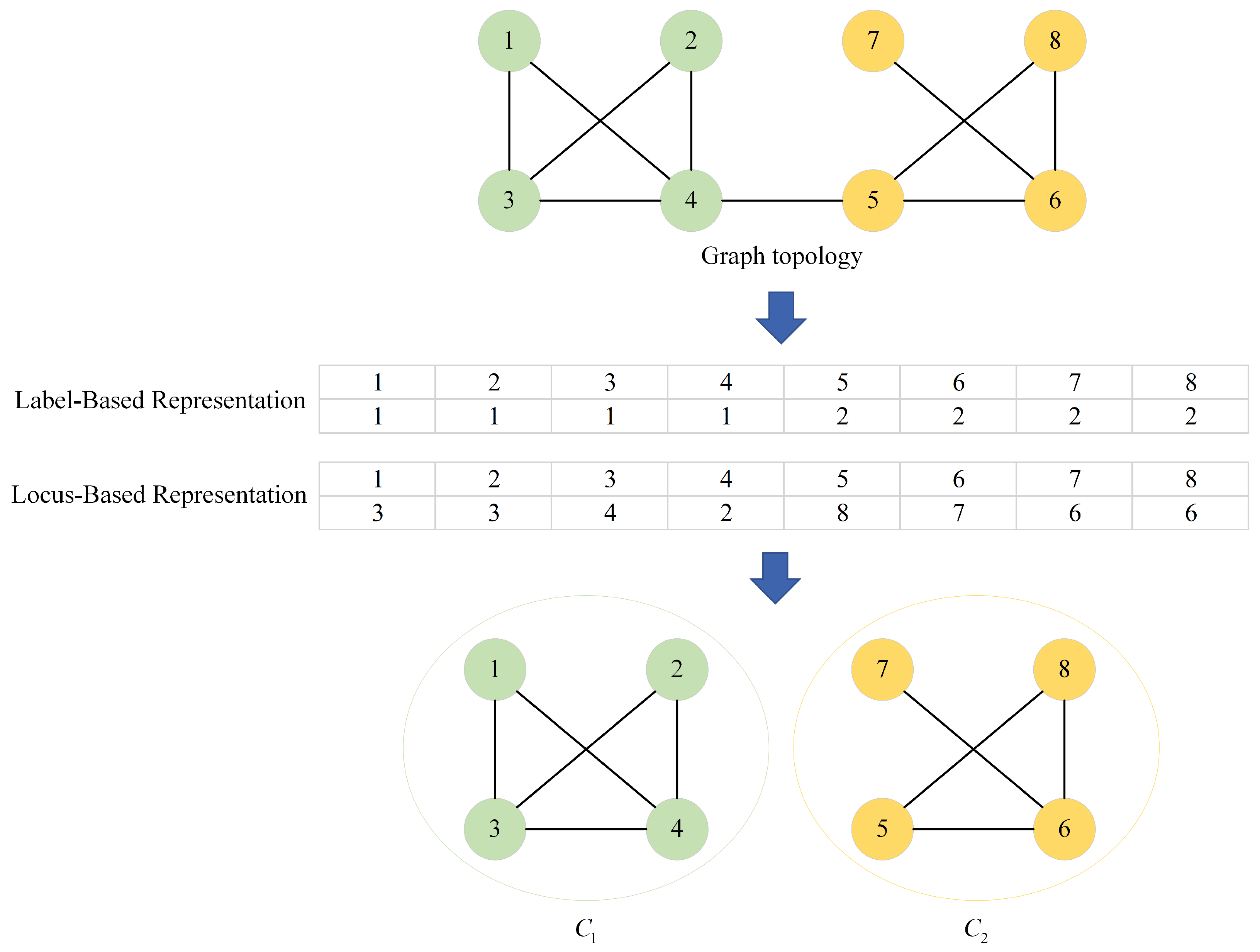
4.1. Representation of Solutions

At this stage, two representation approaches exist in the community discovery domain: the label-based and the locus-based adjacency representation approaches. The two representation approaches consider the solution as a gene, and each gene corresponds to a node in the graph. The locus-based adjacency encoding randomly links each gene bit to a neighbor node in the community, where $Gen{e}_i=j$ indicates that there exists a link edge between $nod{e}_i$ and $nod{e}_j$. This encoding method can automatically obtain the number of communities by decoding, but the community structure is not clear. The label-based encoding method, the label of each locus, indicates the number of the community. $Gen{e}_i=j$ means that $nod{e}_i$ belongs to $Cluste{r}_j$ if the label of two nodes $Gen{e}_i=Gen{e}_k$ means that $nod{e}_i$ and $nod{e}_k$ are members of a community. However, the label-based encoding has the disadvantage of redundancy. The representation of the two solutions is shown in Figure 5.

In this paper, we choose representation based on the label-based representation, with the benefit of easy visual access to the community structure. It is important to note that the traditional label-based representation approach may have redundancy. For example, individual $\left[1,1,1,2,2,2\right]$ and individual $\left[0,0,0,1,1,1\right]$ characterize the same community structure. This situation leads to the possibility that the information passed from individual $x_{gbest}$ to individual $x_i$ may be somewhat misleading. To address this situation, a label normalization operation is designed to force the labels of each individual to be recoded while keeping the community structure unchanged. The idea of label normalization: follow the community structure in the original individual, and re-assign labels according to the community structure starting from 0 in node order. The label normalization algorithm pseudo-code is as follows Algorithm 2.

Algorithm 2 Pseudo-code for tag normalization.
begin
Input:  $x_i$
1:	Get the set of nodes $S=\left\{v_1,v_2,\cdots ,v_n\right\}$
2:	while  $S\ne \varnothing$  do
3:	Query the label of the smallest node of S$\to labe{l}_{min}$
4:	$t=0$
5:	for each node in $x_i$ do
6:	if $labe{l}_{node}==labe{l}_{min}$ then
7:	$labe{l}_{node}=t$
8:	Delete nodes from S
9:	end if
10:	end for
11:	$t=t+1$
12:	end while
Output: $x_i$.

Suppose an individual is denoted as $\left[3,3,3,3,2,2,2,2\right]$ and the set of nodes $S=\left[1,2,3,4,5,6,7,8\right]$. The label of the smallest node $v_1$ is 3. Iterate through each node in the individual and recode nodes labeled 3 to 0. Remove the nodes from the set S, $S=\left[5,6,7,8\right]$. At this point, the label of the smallest node $v_5$ in S is 2. Iterate through each node in the individual and recode nodes labeled 2 as 1. The nodes are removed from the set S and the final labeled normalized individual representation is obtained as $\left[0,0,0,0,1,1,1,1\right]$.

4.2. Population Initialization

The initialization effect of the population information is crucial for algorithm optimization, and a good initialization scheme can accelerate the accuracy and convergence speed of the algorithm. Oriented to different coding methods, the initialization strategy of the population is different. Most of the label-based coding methods use label propagation strategy to initialize the population, and literature [15] proposes Population Generation via Label Propagation (PGLP). Although the PGLP method can generate higher-quality individuals in the population, it also has two problems: first, the diversity of the population is poor. After extensive experiments, it was found that most of the individuals in the population were initialized to generate exactly the same solution. Secondly, the complexity of the PGLP algorithm is high. As described in reference [15], after the authors’ experiments, it was found that the initialization results tended to be stable after roughly five iterations. Therefore, the final complexity of the algorithm is $O(po{p}_{size}\ast n\ast l)$, where $po{p}_{size}$ is the number of populations, n is the number of nodes in the network, and l is the number of neighbors of each node. Oriented to the network with a small average degree, l can also be ignored.

A new population initialization strategy is designed for the above proposed problem, and the pseudo-code of the algorithm is shown below. First, key nodes in the network are identified, and the number of communities in the initialization phase is decided based on the number of key nodes. Secondly, labels are assigned to the gene loci corresponding to the key nodes in the population individuals. Then label propagation is performed on the neighboring nodes of the key nodes. If a node has a connection relationship with only one key node, the label of the node is equal to the label of the key node; if a node has a connection relationship with multiple key nodes at the same time, the node randomly selects the label of one key node. Finally, labels are assigned to other nodes remaining in the network. The similarity between other nodes and all key nodes is calculated, and the label of the key node with the highest similarity is assigned to that node. The similarity is calculated using Jaccard similarity as follows:

$$Similarity={\displaystyle \frac{\left|A\cap B\right|}{|A\cup B|}}={\displaystyle \frac{\left|A\cap B\right|}{\left|A\right|+\left|B\right|-\left|A\cap B\right|}}$$

(21)

where A,B denote the set of neighboring nodes of the two nodes. The pseudo-code of the algorithm is shown in Algorithm 3.

Algorithm 3 Pseudo-code for population initialization.
begin
Input: Network topology G, population size $po{p}_{size}$
1:	$KV=\varnothing$
2:	Calculate the network average degree $d_{avg}$
3:	$S\leftarrow$Identify nodes in network G with node degree greater than $d_{avg}$
4:	while  $S\ne \varnothing$  do
5:	$Kv\leftarrow$Filter the node $Kv$ with the largest node degree from S
6:	$neighbor\left(Kv\right)\leftarrow$ Identify the neighbor nodes of node $Kv$ located in the set S
7:	$KV=KV\cap Kv$
8:	$S\leftarrow$ Remove nodes in $neighbor\left(Kv\right)$ from S
9:	end while
10:	for  $i=1:po{p}_{size}$  do
11:	Labeling of key nodes
12:	Assigning labels to neighboring nodes of key nodes
13:	Calculate the similarity between the remaining nodes and all key nodes
14:	Assign labels to the remaining nodes and select the label of the key node with the greatest similarity
15:	end for
Output: population information $po{p}_x$.

4.3. Fitness Computation

The selection of the fitness function affects the direction and results of the optimization of the SWO-Net algorithm, and the desired objective function should be a set that can characterize the quality of the community structure with contradictory attributes. The kernel k-means (KKM) function [31] as well as the ratio cut (RC) function [32] are chosen as the fitness function for the SWO-Net algorithm. The expressions of the RC function and the KKM function are as follows:

$$\left\{\begin{array}{c}KKM=2\left(n-k\right)-\sum _{i=1}^k\left({\displaystyle \frac{L\left(V_i,V_i\right)}{\left|V_i\right|}}\right)\hfill \\ RC={\sum }_{i=1}^k\left({\displaystyle \frac{L\left(V_i,\overline{V_i}\right)}{\left|V_i\right|}}\right)\hfill \end{array}\right.$$

(22)

where k denotes the number of communities, $L\left(V_i,V_i\right)$ denotes the number of edges within the same community, and $L\left(V_i,\overline{V_i}\right)$ denotes the number of inter-community edges.

At this stage, there is no clear definition of a community, and the widely recognized description of a community is that it is densely connected with intra-community edges and sparsely connected with inter-community edges. In short, the greater the number of edges within a community and the fewer the number of edges between communities, the better the final community structure. Following this criterion, the KKM function and the RC function are chosen. The KKM function roughly characterizes the total number of edges in the network minus the number of edges within the community, and hence the expectation of dense connectivity within the community can be achieved by minimizing the KKM. The RC function characterizes the number of inter-community edges in the network, so the expectation of sparse inter-community connections can be achieved by minimizing the RC function. Optimization is performed with the help of the above two functions to make the final output community structure as close to the real community as possible.

4.4. Search Strategy

The SWO algorithm simulates spider wasp searching or following, nesting and mating behaviors to update information on the population. Since the three updating strategies are oriented towards continuous optimization of updates, discretization of the three updating strategies is required when dealing with the community discovery problem.

The search and follow behavior of the SWO algorithm is to randomly select two individuals from the population to perform the initial update according to Equation (8); this operation is mainly to expand the search range of the population, but at the same time increase many useless searches. In order to retain the advantage of expanding the search range of the population while reducing the probability of useless search, this study abandons the random selection of individuals operation. The specific method is to utilize the fast non-dominated sort of NSGA-II algorithm species to select two individuals from the mutually non-dominated rank layer. The selected individuals have better fitness values and also reduce the useless search. The mathematical expression of the search behavior is as follows:

$$x_i^{t+1}=x_i^t\otimes \left(x_a^t\oplus x_b^t\right)$$

(23)

where a and b are two individuals randomly selected from the mutually non-dominated individuals in the fast non-dominated sort. The ⊕ is a dissimilarity operation. ⊗ does not denote the kronecker product here; it denotes an update strategy based on neighbor labeling.

The search and follow behavior update process is shown in Figure 6, assuming that the individuals in the rank[0] layer obtained after fast non-dominated sorting contain $\{1,3,4,5,9,\cdots \}$, and the randomly selected individuals are $x_3$ and $x_9$. The matrix obtained after the dissimilarity operator for the existence of gaps in the node community labels is $[0,0,0,1,1,0,0,0]$, which indicates that the two nodes $v_4$ and $v_5$ need to be updated, and the labels of the other nodes whose dissimilarity operator results in 0 do not need to be updated on the contrary. Update $v_4$ based on neighbor labels, $labe{l}_{2,3}=1$ and $labe{l}_{5,6}=0$. The nodes with the highest number of neighbor labels are 0 and 1; at this time, randomly select one of them as the new label of $v_4$. To update $v_5$ based on neighbor labels, $labe{l}_5=1$ and $labe{l}_{6,7,8}=0$, the highest number of neighbor labels is 0, so $labe{l}_5=0$.

The nesting behavior of the SWO algorithm mainly involves individuals choosing the best nesting location under the guidance of the best individual, and the redefined update formula incorporates the in-population consensus community, and the individuals will move under the joint guidance of the global optimal individual and the in-population consensus community. The global optimal individual with the highest NMI value is the global optimal solution. The new nesting behavior process is shown in Figure 7.

Assuming globally optimal individuals $x_{gbest}=[1,1,1,0,1,0,0,0]$, $x_i=[1,1,1,2,2,0,0,0]$. The community structures $x_{gbest}=\left\{\left\{1,2,3,5\right\},\left\{4,6,7,8\right\}\right\}$ and $x_i=\left\{\left\{1,2,3\right\},\left\{4,5\right\},\left\{6,7,8\right\}\right\}$ are obtained by decoding. The intra-population consensus community is $\left\{\left\{1,2,3\right\}\left\{6,7,8\right\}\right\}$. Iterate through each of the consensus community. Pass the labeling information of the community $\left\{1,2,3,5\right\}$ with $\left\{1,2,3\right\}$ in $x_{gbest}$ to the $x_i$ individual, and the final updated $x_i=\left[1,1,1,1,2,1,0,0,0\right]$. Compare the updated $x_{new}$ with $x_i$, and if it dominates $x_i$, keep it; otherwise, discard it. The same operates on $\{6,7,8\}$ in the consensus community for dominance degree comparison and ultimately the individual movement updates under nesting behavior.

The mating behavior of the SWO algorithm is redefined by the crossover operator. In the SWO algorithm, male spider wasps are not involved in the process of the searching and tracking and nesting behavior, so a male individual needs to be selected when performing the mating behavior. When discretizing the SWO algorithm, it is also necessary to select one of the many individuals as the male to cross with the female. Here, we refer to the two-point crossover approach in the MOPSO-Net algorithm to generate offspring, while selecting the better individuals to be retained through dominance degree matching. Meanwhile, considering the convergence of the algorithm in the later stage, the two-point crossover may destroy the genes of the excellent parent, so after generating the offspring, the offspring individuals are matched with the parent individuals in the degree of dominance, and the optimal individuals are retained as the new offspring individuals as a way to ensure the convergence of the algorithm. In summary, the overall framework of SWO-Net algorithm is given as shown in Algorithm 4.

Algorithm 4 Pseudo-code for the SWO-Net algorithm.
begin
Input: Dynamic network: $G=\left\{G_1,G_2,\cdots ,G_T\right\}$, Population size: $po{p}_{size}$, the maximum number of iterations: $ge{n}_{max}$
1:	Initializing intra-population consensus community
2:	for  $t=1:T$  do
3:	Initialize population information $po{p}^t=\left\{x_1,x_2,\cdots ,x_{po{p}_{size}}\right\}$
4:	Compute the global optimal solution $bes{t}_g$
5:	while $gen<ge{n}_{max}$ do
6:	Calculate the KKM and RC values for all individuals in $po{p}^t$
7:	for $j=1:po{p}_{size}$ do
8:	Update population location information
9:	Perform label normalization
10:	Update the global optimal solution $bes{t}_g$
11:	end for
12:	if $gen\%5==0$ then
13:	Calculating inter-population consensus community and updating population information
14:	Updating the global optimal solution $bes{t}_g$
15:	end if
16:	end while
17:	Computing intra-population consensus community
18:	end for
Output: The optimal community structure $bes{t}_g$ for each network $G_i$.

4.5. Computational Complexity

Suppose n is the number of nodes in the network, m is the number of edges in the network, the maximum node degree of the network is D, $ge{n}_{max}$ is the maximum number of iterations, $po{p}_{size}$ is the population size, and k is the maximum number of communities. The computational complexity of the SWO-Net algorithm can be obtained by calculating the complexity of the above algorithmic process for each time step t. In the first step, the initialization algorithm consists of key node identification and label assignment, where the computational complexity of the key node algorithm is $O\left(n^{\prime }\times D\right)$, where $n^{\prime }$ is the number of nodes in the network whose node degree exceeds the average node degree. The label assignment can be performed in linear time, so the complexity of the first part of the algorithm is $O\left(n^{\prime }\times D+po{p}_{size}\times n\right)$. In the second step (steps 5–15), for each solution, the complexity of the computation process of KKM and RC values is $O\left(m+n\right)$, so the complexity of step 6 is $O\left(po{p}_{size}\times \left(m+n\right)\right)$. The complexity of steps 7–10 is $O\left(po{p}_{size}\times n\times k\right)$. In steps 11–18, the inter-population consensus community needs to be computed, and its computational complexity is $O\left(po{p}_{size}\times n\times k\right)$. The computational complexity of the remainder is $O\left(n^2\right)$. The computational complexity of the SWO-Net algorithm is $O\left(ge{n}_{max}\times po{p}_{size}\times \left(m+nk\right)+n^2\right)$.

5. Experiment

We compare the SWO-Net algorithm with six popular algorithms and the latest algorithms including the FaceNet algorithm [33], the Kim-Han algorithm [34], the Infomap algorithm [35], the MODPSO algorithm [36], the DYNMOGA [20] algorithm, the sE-NMF algorithm [37], and the MOCCD algorithm [38]. We evaluate the performance of the proposed algorithms. Several methods are used for comparison, typical of different types of algorithms. The FaceNet and Kim-Han algorithms are typical evolutionary clustering methods, MODPSO is an excellent method in dealing with static network community discovery problems, the Algorithm DYNMOGA and MOCCD algorithms are outstanding algorithms for multi-objective evolutionary computational methods, sE-NMF is based on a semi-supervised evolutionary non-negative matrix factorization method, and the Infomap algorithm is a superior performance community detection framework.

5.1. Experimental Environment and Parameter Settings

This experiment is implemented on pycharm 2022. The algorithms rely on a computer with Intel® CoreTM i5 CPU 2.67 GHz and 16 GB (14 GB usable) of memory configuration. Each method was run independently 20 times on each network and the three results, best, average and standard deviation, are recorded for the relevant evaluation metrics.

The parameter settings of the relevant comparison algorithms are suggested in references [20,33,37]. The parameter $\alpha$ in the FaceNet is set to 0.8 according to the literature. The population size $po{p}_{size}$ is set to 100 and the maximum number of iterations $ge{n}_{max}$ is set to 100 for the DYNMOGA, MODPSO, MOCCD and the SWO-Net algorithms. The DYNMOGA algorithm also involves crossover rate and variance rate parameters, where the crossover rate is set to 0.8, and the variance rate is set to 0.2 according to Pizzuti’s recommendations. The three key parameters $\alpha$, $\beta$, and $\gamma$ in the sE-NMF algorithm are set to 0.8, 0.95, and 0.1, respectively. In the MOCCD algorithm, the parameter $r^{\prime }$ is set to 0.8, and $\gamma$ is set to 0.2. In the SWO-Net algorithm, the minimum support threshold $T_{MS}$ is set to 0.7. Every ten iterations, a consensus community between populations is voted on by the group, and the consensus portion is inserted into the population.

5.2. Evaluation Metric

To evaluate the performance of the MOPIO-Net algorithm with other baseline algorithms in the community detection problem, we choose NMI (Normalized Mutual Information) as the evaluation metric. The NMI measures the similarity between the real community structure of the network and the community structure identified by the algorithm. The more similar the community structure identified by the algorithm is to the real community structure, the closer the value of NMI is to 1; on the contrary, the value of NMI is close to 0. The value of $NMI\in \left[0,1\right]$. Suppose, the real community structure partition is $D=\left\{D_1,D_2,\cdots D_q\right\}$, and the community structure partition identified by the algorithm is $E=\left\{E_1,E_2,\cdots ,E_p\right\}$, where q and p denote the number of communities in the real partition D and the algorithm’s partition E, respectively. By introducing the confusion matrix C and calculating the similarity of the two partitions, the NMI can be defined as

$$NMI={\displaystyle \frac{-2{\sum }_{i=1}^{C_D}{\sum }_{j=1}^{C_E}{C}_{ij}log\left(C_{ij}N/\phantom{C_{ij}N{C}_{i.}{C}_{.j}}{C}_{i.}{C}_{.j}\right)}{{\sum }_{i=1}^{C_D}{C}_{i.}log\left(C_{i.}/\phantom{C_{i.}N}N\right)+{\sum }_{j=1}^{C_E}{C}_{.j}log\left(C_{.j}/\phantom{C_{.j}N}N\right)}}$$

(24)

where $C_{D\left(E\right)}$ denotes the number of communities in partition $D\left(E\right)$, $C_{i.\left(.j\right)}$ denotes the sum of the elements in row i (column j) of the confusion matrix, and N denotes the number of nodes in the network.

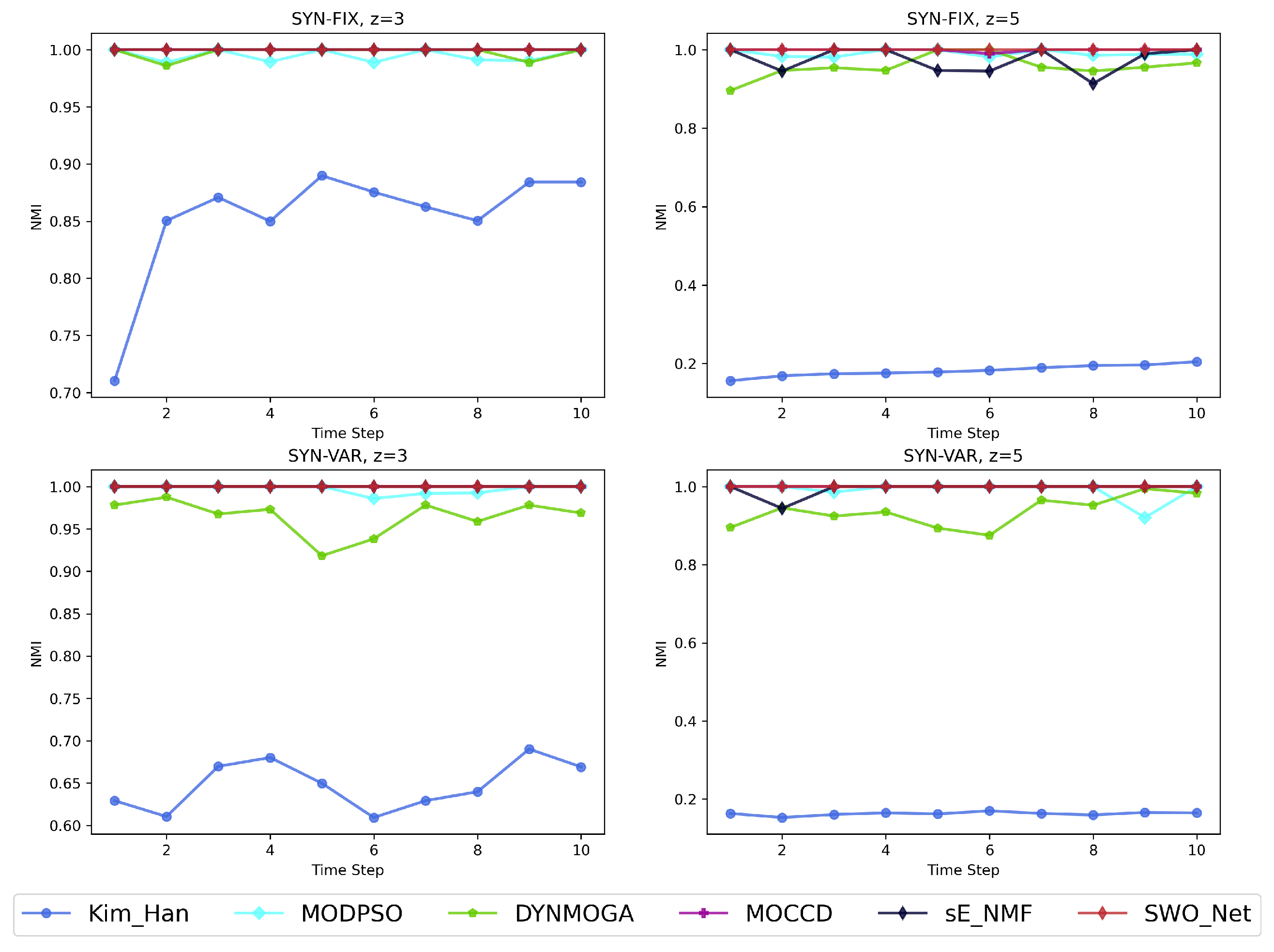
5.3. Experimental Results of the Synthetic Networks

In this section, the SWO-Net algorithm is tested against other comparative algorithms for algorithmic performance on synthetic networks. The experiments are tested on two synthetic datasets where the community segmentation results are known.

Dataset 1: Referring to the synthetic dataset characterization proposed by Greene et al. [39], in this paper, we use the dynamic benchmark network generator to synthesize the networks. Each synthetic network contains 10 time steps, and each network is set up with 1000 nodes, with nodes having an average degree of 15, a maximum degree of 50, and a mixing parameter of 0.2, and the number of communities ranging between 25 and 50. The evolutionary properties of dynamic networks are characterized by four types of evolutionary events: births and deaths, expansions and contractions, intermittent communities, and mergers and splits.

(1) Births and deaths: 10% of new communities are created by removing nodes from other communities in each time step of the dynamic network, and 10% communities are randomly removed in the final step.

(2) Expansion and Collapse: at each time step of the dynamic network, 10% of the communities are expanded or collapsed by randomly selecting them and letting the communities expand or collapse by 25% of their own size. When expanding, new nodes are randomly selected from other communities.

(3) Intermittent communities: in each time step of a dynamic network, 10% of the communities are hidden in the first step.

(4) Merging and splitting: at each time step of the dynamic network, 10% of the communities are chosen to be split and another 10% are chosen to merge.

Figure 8 depicts the NMI values of the SWO-Net algorithm with respect to the benchmark algorithm, and it can be clearly seen that the SWO-Net algorithm has the best overall performance on the four datasets. Meanwhile, in the dynamic evolution of the network over time, the NMI values of the FaceNet algorithm, MODPSO algorithm, and MYNMOGA algorithm decrease sharply with the evolution process, while the sE-NMF algorithm and MOCCD algorithm are more stable.

Dataset 2: The dataset introduced in reference [34] is used. This dataset contains the SYN-FIX dataset and the SYN-VAR dataset, where the SYN-FIX dataset changes the node’s original community at each time step, but the number of communities is constant at each time step. The SYN-VAR dataset simulates the evolutionary events of node births and deaths, while the number of communities in the network is variable at each time step. The SYN-FIX dataset is composed of 128 nodes in 4 communities, each containing 32 nodes. Each node has an average degree of 16 and is connected to z nodes outside the community to which it belongs. The value of the parameter z determines the degree of fuzziness of the network. When $z=3$, the network has a clear community structure, i.e., more tightly connected within communities and sparsely connected between communities. When $z=5$, the community structure becomes ambiguous and complex due to the increased number of inter-community connections. In order to highlight the dynamic evolutionary characteristics of the network, the network at time step $t+1$ follows the smoothing property, overproduced by the network at time step t. This is performed by randomly selecting 3 nodes from each community in the $G_t$ network and then reallocating the 12 nodes to 4 random communities.

The SYN-VAR dataset is generated in a different way from the SYN-FIX dataset, which is formed through operations such as generating and dissolving communities, and adding and removing nodes. The initial SYN-VAR network consists of 256 nodes, all of which form four communities, each with 64 nodes. The parameter z functions in the SYN-VAR dataset in the same way as it does in the SYN-FIX dataset as a variable for network fuzzy control. In order to generate 10 consecutive networks, a new community is generated by randomly selecting 8 nodes from each community within the first 5 consecutive time steps and using these 32 nodes. The process lasts a total of 5 time steps, and at the end of the 5 time steps, the nodes will return to their original communities, and the number of network communities is gradually restored to the initial moment. Thus, the number of communities in the network at each of the 10 time steps varies as 4, 5, 6, 7, 8, 8, 7, 6, 5, 4. The average degree of each node in the community is set to one-half of the number of nodes in the community. In addition, in each time step, 16 nodes are randomly removed from the network, while 16 new nodes are generated.

Figure 9 illustrates the NMI values of the algorithm recognition results for the six algorithms under the SYN-FIX dataset and SYN-VAR dataset with parameter z of 3 and 5, respectively. From the figure, it can be seen that among the four networks, the Kim-Han algorithm has the worst performance, and there is a large gap with the other algorithms. The DYNMOGA algorithm performs equally poorly, but the gap with the MODPSO algorithm, the MOCCD algorithm, the sE-NMF algorithm and the SWO-Net algorithm is small. Among the remaining algorithms, the proposed SWO-Net algorithm performs the best and is the most stable. When oriented towards the SYN-FIX dataset and the SYN-VAR dataset, SWO-Net accurately identifies the community structure of the network regardless of what value z takes. The MOCCD algorithm, the MODPSO algorithm, and the sE-NMF algorithm have small differences in performance, but evaluated from the point of view of the algorithm’s own adaptability, the sE-NMF algorithm needs to continuously adjust the parameters to adapt to different network models.

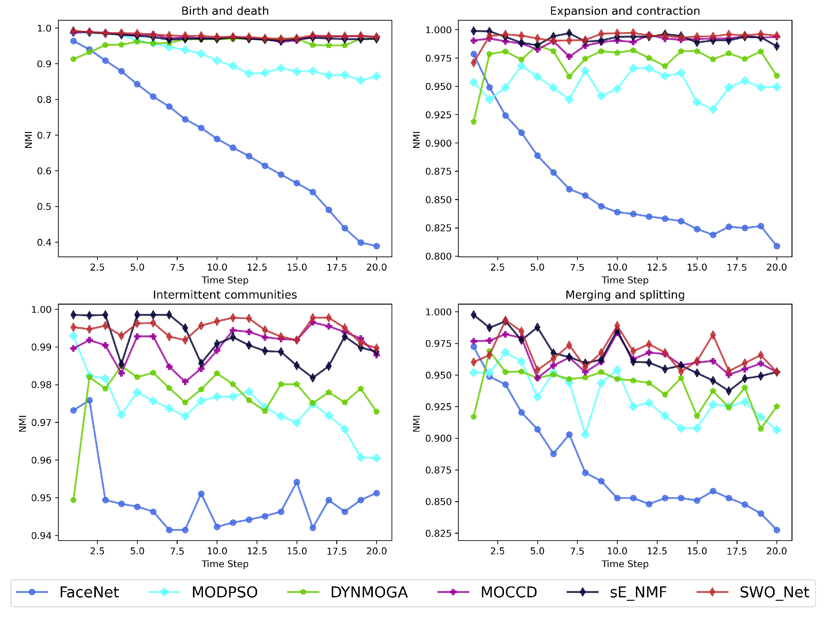
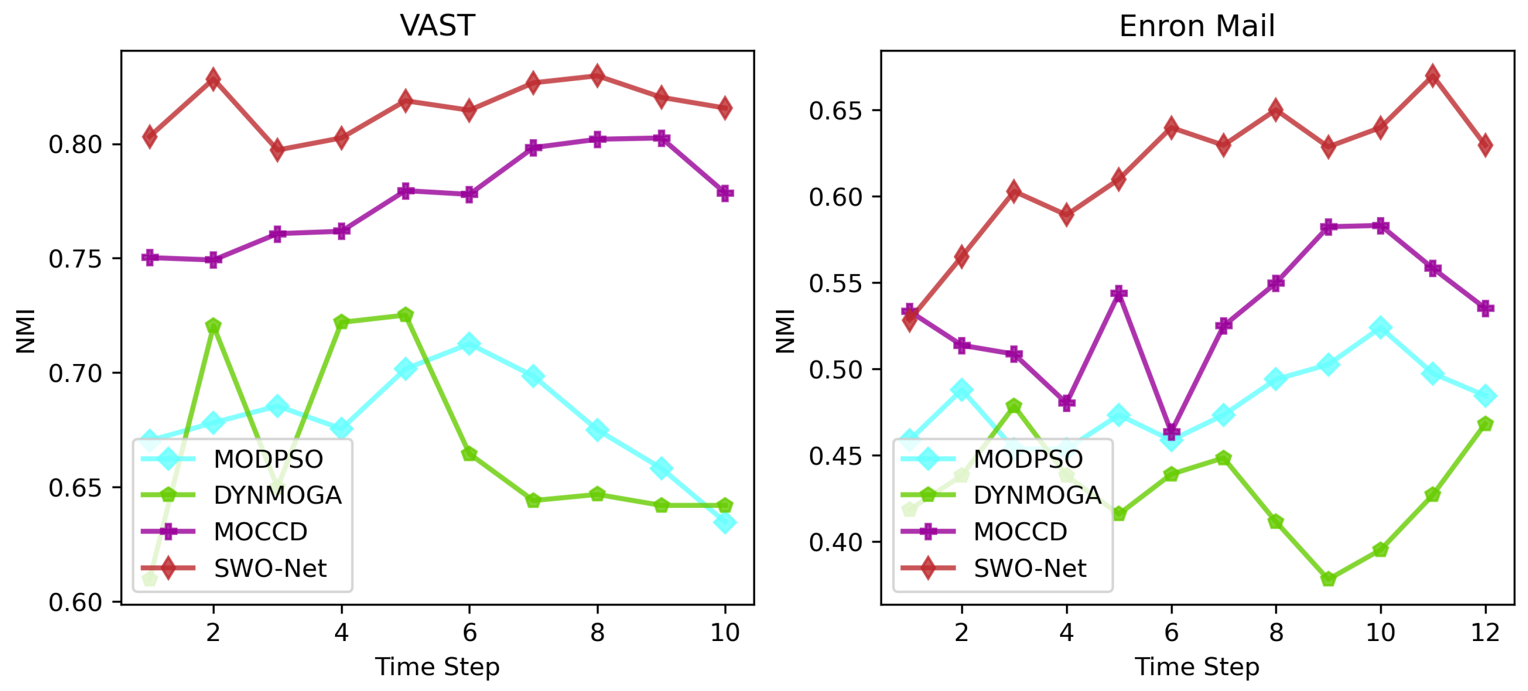
5.4. Experimental Results on the Real Networks

The real community structure of the network at different time steps is embedded in the synthetic data used in the previous subsection. In Section 2, real-world VAST datasets and Enron dataset are selected. Since it is not possible to know the real node affiliation, the experiments in this section use the same operations as in the FaceNet algorithm as well as in the DYNMOGA algorithm. All networks within a time step are merged into a single network, and then the clustering results of the merged network (generated by Infomap) are used as the true cluster results.

(1) VAST dataset: The VAST dataset is derived from an event task in the IEEE VAST 2008 Challenge, and the dataset selected for this experiment is a task in the IEEE VAST 2008 Mini Challenge 3. This task contains cell phone call records for a 10-day period in mid-June, 2006. A total of 400 phone numbers are used to generate 9834 call records by calling each other in 10 days with a time step of 10. Each unique number corresponds to a node in the network, and the call records generated between two phone numbers serve as a connecting edge between two nodes in the network. The chosen dataset can be downloaded from https://www.cs.umd.edu/hcil/VASTchallenge08/ (accessed on 13 February 2023).

(2) Enron Mail dataset: The Enron dataset consists of mail from 1999 to 2002 provided by Enron, a U.S.-based company. In this network, the employees of the organization are considered nodes in the network, and the email exchanges between employees are considered connections in the network. Emails between employees of Enron Enterprises for the year 2001 are intercepted, and this is because in the middle of the year 2001, the emails between employees were the closest, and the number of emails was the highest. In order to better delineate the time step, the month in which the emails were sent is used as a cut-off to divide the 2001 employee email exchanges into 12 parts corresponding to the months of January–December. The Enron Mail dataset is available from https://www.cs.cmu.edu/~enron/ (accessed on 13 February 2023). The details of the above two real network datasets are shown in

Table 1. The statistical information on the VAST dataset.

T	$\left|\mathit{C}\right|$	$\left|\mathit{V}\right|$	$\left|\mathit{E}\right|$	${\left|\mathit{E}\right|}^{*}$	${\mathit{D}}_{\mathbf{avg}}$
1	32	370	987	525	2.625
2	35	373	964	499	2.495
3	30	374	953	509	2.545
4	31	374	1013	514	2.57
5	32	373	991	508	2.54
6	25	373	963	512	2.56
7	33	367	936	498	2.49
8	36	365	1005	511	2.555
9	34	374	982	518	2.59
10	32	384	1040	530	2.65

where T denotes the time step; $\left|C\right|$ denotes the number of communities; $\left|V\right|$ denotes the number of nodes in the network; $\left|E\right|$ denotes the number of connections in the network; ${\left|E\right|}^{*}$ denotes the connections between two members generated through different calls; and $D_{avg}$ denotes the average degree of the network.

As shown in Figure 10, the SWO-Net algorithm has the best performance in the VAST dataset, as the NMI value of SWO-Net algorithm is higher than that of the MODPSO algorithm, DYNMOGA algorithm, and MOCCD algorithm over time. In the Enron dataset, the complexity of the Enron dataset is much higher than the VAST dataset, as can be seen by the number of nodes and connections and the average degree of the network in

Table 2. The statistical information on the Enron Mail dataset.

T	$\left|\mathit{C}\right|$	$\left|\mathit{V}\right|$	$\left|\mathit{E}\right|$	${\left|\mathit{E}\right|}^{*}$	${\mathit{D}}_{\mathbf{avg}}$
1	11	96	1070	180	2.3841
2	7	93	1559	204	2.702
3	12	97	1844	218	2.8874
4	12	108	1869	257	3.404
5	15	125	1919	292	3.8675
6	10	120	1001	231	3.0596
7	10	109	1325	252	3.3377
8	9	131	2270	396	5.245
9	10	128	3152	361	4.7815
10	13	135	8693	575	7.6159
11	9	127	6276	469	6.2119
12	8	113	2146	325	4.3046

. From the NMI values, it can be found that the NMI values of each algorithm in the Enron dataset have different degrees of decline compared to those of the VAST network, indicating that the algorithms still need to improve their ability to deal with highly fuzzy structured networks. However, in the Enron dataset, the SWO-Net algorithm continues to outperform the MODPSO algorithm and the MYNMOGA algorithm, as well as the MOCCD algorithm in terms of NMI values. The superior performance of the SWO-Net algorithm is confirmed.

6. Conclusions

In this paper, a novel SWO-Net algorithm for detecting dynamic network community structures is proposed. First, the coding method, initialization method, and update strategy of population individuals of the SWO algorithm are discretized to adapt to the community detection problem. Second, the concept of intra-population and inter-population consensus community is proposed, which enables the population to maintain a certain degree of continuity in the process of evolution through the transfer of information from the consensus community in the process of population evolution, and by doing so, the optimization of the time and space loss required for evolution is achieved. In simulation comparison experiments, the performance of the algorithm is verified by comparing it with other excellent benchmark algorithms in synthetic networks and real-world dynamic networks. The statistical results show that the SWO-Net algorithm outperforms other benchmark algorithms, verifying the feasibility and effectiveness of the SWO-Net algorithm in dealing with the field of dynamic network community detection.

References

1. Fortunato, S. Community detection in graphs. Phys. Rep. 2010, 486, 75–174. [Google Scholar] [CrossRef]
2. Yu, L.; Guo, X.; Zhou, D.; Zhang, J. A Multi-Objective Pigeon-Inspired Optimization Algorithm for Community Detection in Complex Networks. Mathematics 2024, 12, 1486. [Google Scholar] [CrossRef]
3. Rostami, M.; Berahmand, K.; Forouzandeh, S. A novel community detection based genetic algorithm for feature selection. J. Big Data 2021, 8, 2. [Google Scholar] [CrossRef]
4. Moradi, P.; Ahmadian, S.; Akhlaghian, F. An effective trust-based recommendation method using a novel graph clustering algorithm. Phys. A Stat. Mech. Its Appl. 2015, 436, 462–481. [Google Scholar] [CrossRef]
5. Rezaeimehr, F.; Moradi, P.; Ahmadian, S.; Qader, N.N.; Jalili, M. TCARS: Time-and community-aware recommendation system. Future Gener. Comput. Syst. 2018, 78, 419–429. [Google Scholar] [CrossRef]
6. Wang, Z.; Wu, Y.; Li, Q.; Jin, F.; Xiong, W. Link prediction based on hyperbolic mapping with community structure for complex networks. Phys. A Stat. Mech. Its Appl. 2016, 450, 609–623. [Google Scholar] [CrossRef]
7. Deng, X.; Wen, Y.; Chen, Y. Highly efficient epidemic spreading model based LPA threshold community detection method. Neurocomputing 2016, 210, 3–12. [Google Scholar] [CrossRef]
8. Wang, S.; Gong, M.; Liu, W.; Wu, Y. Preventing epidemic spreading in networks by community detection and memetic algorithm. Appl. Soft Comput. 2020, 89, 106118. [Google Scholar] [CrossRef]
9. Fortunato, S.; Barthelemy, M. Resolution limit in community detection. Proc. Natl. Acad. Sci. USA 2007, 104, 36–41. [Google Scholar] [CrossRef]
10. Pizzuti, C. Evolutionary computation for community detection in networks: A review. IEEE Trans. Evol. Comput. 2017, 22, 464–483. [Google Scholar] [CrossRef]
11. Li, Z.; Zhang, S.; Wang, R.S.; Zhang, X.S.; Chen, L. Quantitative function for community detection. Phys. Rev. E-Stat. Nonlinear Soft Matter Phys. 2008, 77, 036109. [Google Scholar] [CrossRef] [PubMed]
12. Arenas, A.; Duch, J.; Fernández, A.; Gómez, S. Size reduction of complex networks preserving modularity. New J. Phys. 2007, 9, 176. [Google Scholar] [CrossRef]
13. Shen, H.; Cheng, X.; Cai, K.; Hu, M.B. Detect overlapping and hierarchical community structure in networks. Phys. A Stat. Mech. Its Appl. 2009, 388, 1706–1712. [Google Scholar] [CrossRef]
14. Pizzuti, C. Ga-net: A genetic algorithm for community detection in social networks. In International Conference on Parallel Problem Solving from Nature; Springer: Berlin/Heidelberg, Germany, 2008; pp. 1081–1090. [Google Scholar]
15. Gong, M.; Fu, B.; Jiao, L.; Du, H. Memetic algorithm for community detection in networks. Phys. Rev. E-Stat. Nonlinear Soft Matter Phys. 2011, 84, 056101. [Google Scholar] [CrossRef] [PubMed]
16. Pizzuti, C. A multiobjective genetic algorithm to find communities in complex networks. IEEE Trans. Evol. Comput. 2011, 16, 418–430. [Google Scholar] [CrossRef]
17. Rahimi, S.; Abdollahpouri, A.; Moradi, P. A multi-objective particle swarm optimization algorithm for community detection in complex networks. Swarm Evol. Comput. 2018, 39, 297–309. [Google Scholar] [CrossRef]
18. Palla, G.; Barabási, A.L.; Vicsek, T. Quantifying social group evolution. Nature 2007, 446, 664–667. [Google Scholar] [CrossRef] [PubMed]
19. Sun, Z.; Sheng, J.; Wang, B.; Ullah, A.; Khawaja, F. Identifying communities in dynamic networks using information dynamics. Entropy 2020, 22, 425. [Google Scholar] [CrossRef]
20. Folino, F.; Pizzuti, C. An evolutionary multiobjective approach for community discovery in dynamic networks. IEEE Trans. Knowl. Data Eng. 2013, 26, 1838–1852. [Google Scholar] [CrossRef]
21. Paul, S.; Koner, C.; Mitra, A.; Ghosh, S. A Study on Algorithms for Detection of Communities in Dynamic Social Networks: A Review. In International Conference on Computational Intelligence in Communications and Business Analytics; Communications in Computer and Information Science (1956); Dasgupta, K., Mukhopadhyay, S., Mandal, J., Dutta, P., Eds.; Springer: Kalyani, India, 2023; pp. 51–64. [Google Scholar]
22. Chakrabarti, D.; Kumar, R.; Tomkins, A. Evolutionary clustering. In Proceedings of the 12th ACM SIGKDD International Conference on Knowledge Discovery and Data Mining, Philadelphia, PA, USA, 20–23 August 2006; pp. 554–560. [Google Scholar]
23. Kherad, M.; Dadras, M.; Mokhtari, M. Community detection based on influential nodes in dynamic networks. J. Supercomput. 2024, 80, 24664–24688. [Google Scholar] [CrossRef]
24. Ranjkesh, S.; Masoumi, B.; Hashemi, S.M. A novel robust memetic algorithm for dynamic community structures detection in complex networks. World Wide Web 2024, 27, 3. [Google Scholar] [CrossRef]
25. Zhou, T.; Pan, R.; Zhang, J.; Wang, H. An attribute-based Node2Vec model for dynamic community detection on co-authorship network. Comput. Stat. 2024. [Google Scholar] [CrossRef]
26. Abdel-Basset, M.; Mohamed, R.; Jameel, M.; Abouhawwash, M. Spider wasp optimizer: A novel meta-heuristic optimization algorithm. Artif. Intell. Rev. 2023, 56, 11675–11738. [Google Scholar] [CrossRef]
27. Lancichinetti, A.; Fortunato, S. Consensus clustering in complex networks. Sci. Rep. 2012, 2, 336. [Google Scholar] [CrossRef] [PubMed]
28. Chakraborty, T.; Srinivasan, S.; Ganguly, N.; Bhowmick, S.; Mukherjee, A. Constant communities in complex networks. Sci. Rep. 2013, 3, 1825. [Google Scholar] [CrossRef]
29. Mandaglio, D.; Amelio, A.; Tagarelli, A. Consensus community detection in multilayer networks using parameter-free graph pruning. In Proceedings of the Advances in Knowledge Discovery and Data Mining: 22nd Pacific-Asia Conference, PAKDD 2018, Melbourne, VIC, Australia, 3–6 June 2018; Proceedings, Part III 22. Springer: Berlin/Heidelberg, Germany, 2018; pp. 193–205. [Google Scholar]
30. Chiu, W.Y.; Yen, G.G.; Juan, T.K. Minimum manhattan distance approach to multiple criteria decision making in multiobjective optimization problems. IEEE Trans. Evol. Comput. 2016, 20, 972–985. [Google Scholar] [CrossRef]
31. Angelini, L.; Boccaletti, S.; Marinazzo, D.; Pellicoro, M.; Stramaglia, S. Identification of network modules by optimization of ratio association. Chaos Interdiscip. J. Nonlinear Sci. 2007, 17, 023114. [Google Scholar] [CrossRef] [PubMed]
32. Wei, Y.C.; Cheng, C.K. Ratio cut partitioning for hierarchical designs. IEEE Trans. Comput.-Aided Des. Integr. Circuits Syst. 1991, 10, 911–921. [Google Scholar] [CrossRef]
33. Lin, Y.R.; Chi, Y.; Zhu, S.; Sundaram, H.; Tseng, B.L. Analyzing communities and their evolutions in dynamic social networks. ACM Trans. Knowl. Discov. Data (TKDD) 2009, 3, 1–31. [Google Scholar] [CrossRef]
34. Kim, M.S.; Han, J. A particle-and-density based evolutionary clustering method for dynamic networks. Proc. VLDB Endow. 2009, 2, 622–633. [Google Scholar] [CrossRef]
35. Lancichinetti, A.; Fortunato, S. Community detection algorithms: A comparative analysis. Phys. Rev. E-Stat. Nonlinear Soft Matter Phys. 2009, 80, 056117. [Google Scholar] [CrossRef] [PubMed]
36. Gong, M.; Cai, Q.; Chen, X.; Ma, L. Complex network clustering by multiobjective discrete particle swarm optimization based on decomposition. IEEE Trans. Evol. Comput. 2013, 18, 82–97. [Google Scholar] [CrossRef]
37. Ma, X.; Dong, D. Evolutionary nonnegative matrix factorization algorithms for community detection in dynamic networks. IEEE Trans. Knowl. Data Eng. 2017, 29, 1045–1058. [Google Scholar] [CrossRef]
38. Li, W.; Zhou, X.; Yang, C.; Fan, Y.; Wang, Z.; Liu, Y. Multi-objective optimization algorithm based on characteristics fusion of dynamic social networks for community discovery. Inf. Fusion 2022, 79, 110–123. [Google Scholar] [CrossRef]
39. Greene, D.; Doyle, D.; Cunningham, P. Tracking the evolution of communities in dynamic social networks. In Proceedings of the 2010 International Conference on Advances in Social Networks Analysis and Mining, Odense, Denmark, 9–11 August 2010; IEEE: Piscataway, NJ, USA, 2010; pp. 176–183. [Google Scholar]
Figure 1. Example of dynamic network evolution.
Mathematics 13 00265 g001
Figure 2. Example of an intra-population consensus community.
Mathematics 13 00265 g002
Figure 3. Example of an inter-population consensus community.
Mathematics 13 00265 g003
Figure 4. The flowchart of the SWO-Net algorithm.
Mathematics 13 00265 g004
Figure 5. Two methods of representation.
Mathematics 13 00265 g005
Figure 6. Example of search and follow behavior update.
Mathematics 13 00265 g006
Figure 7. Example of nesting behavior update.
Mathematics 13 00265 g007
Figure 8. Performance comparison of algorithms on dataset 1.
Mathematics 13 00265 g008
Figure 9. The comparison of NMI values of algorithms on SYN-FIX and SYN-VAR datasets.
Mathematics 13 00265 g009
Figure 10. The performance comparison of four algorithms under real-world dynamic networks.
Mathematics 13 00265 g010