A Dual-Path Neural Network for High-Impedance Fault Detection

Abstract

High-impedance fault detection poses significant challenges for distribution network maintenance and operation. We propose a dual-path neural network for high-impedance fault detection. To enhance feature extraction, we use a Gramian Angular Field algorithm to transform 1D zero-sequence voltage signals into 2D images. Our dual-branch network simultaneously processes both representations: the CNN extracts spatial features from the transformed images, while the GRU captures temporal features from the raw signals. To optimize model performance, we integrate the Crested Porcupine Optimizer (CPO) algorithm for the adaptive optimization of key network hyperparameters. The experimental results demonstrate that our method achieves a 99.70% recognition accuracy on a dataset comprising high-impedance faults, capacitor switching, and load connections. Furthermore, it maintains robust performance under various test conditions, including different noise levels and network topology changes.

1. Introduction

Single-phase-to-ground faults constitute approximately 80% of all fault types in distribution networks. Among these, high-impedance faults (HIFs), caused by the contact of overhead lines with materials such as tree branches, cement, sand, or animals, result in ground resistance values ranging from hundreds to thousands of ohms and account for roughly 5% of total fault incidents [1,2,3]. Due to their low current amplitudes, these faults are difficult to detect, often allowing the faulty conditions to persist for 1–2 h. Furthermore, high-frequency electrical signals, such as traveling waves and transients, not only exhibit low amplitudes but are also highly susceptible to noise interference and arc distortions, posing additional challenges to accurate fault detection [4,5,6,7].

Many researchers have conducted in-depth studies on high-impedance fault identification in distribution networks. Current approaches primarily rely on signal processing methods, where the analysis typically involves various electrical parameters including the voltage, current, magnetic field intensity, and impedance. The most commonly employed signal decomposition techniques include Fast Fourier Transform (FFT) [8], Empirical Mode Decomposition (EMD) [9], Hilbert–Huang Transform (HHT) [10], and Wavelet Transform (WT) [11]. For example, V. Gogula et al. [12] developed a high-impedance fault detection method based on the dynamic Hilbert–Huang transform. Their method analyzed three key parameters: instantaneous frequency, RMS value, and crest factor. Zhiwei Yao et al. [13] utilized wavelet transform and energy entropy to capture the transient features of fault signals. Mostafa Satea et al. [14] developed a method to distinguish HIFs from switching events. Their approach combined third harmonic analysis and a wavelet-based algorithm by monitoring changes in the third harmonic magnitude of the zero-sequence voltage and current components. However, their reliance on predefined thresholds and their sensitivity to noise often limit their effectiveness in dynamic and noisy environments. Moreover, real-time implementation remains challenging due to the high computational demands and the variability of fault characteristics in practical systems. Despite these limitations, signal processing methods remain foundational to fault detection and provide a basis for AI-based developments.

Recent advancements in computational capabilities and neural network architectures have significantly enhanced power grid fault detection. Neural networks, known for their excellent feature extraction capabilities under complex conditions, offer promising opportunities for more efficient and reliable fault detection methods. Examples include RESNET [15,16], ANN [17], SqueezeNet [18], and AlexNet [19], which have been applied to improve fault detection accuracy in various contexts. Zheng et al. [20] combined Variational Mode Decomposition (VMD) with the Inception–CNN for high-precision fault-type recognition. Zhang et al. [21] used object detection and attention mechanisms to locate faults from synchronized measurement data. Gogula et al. [22] integrated Discrete Wavelet Transform (DWT) with the Radial Basis Function Neural Network (RBFNN) for processing traveling wave signals. Guo et al. [23] proposed a high-impedance fault detection method using both Time–Frequency Spectrum (TFS) and transfer learning. Liang et al. [24] applied wavelet transform and a CNN for multi-scale feature extraction and classification. Bhatnagar et al. [25] developed an LSTM-based protection scheme for classifying high-impedance and low-impedance faults. Odion et al. [26] used an ANN for fault detection and localization in the Nigerian 330 kV transmission system. Overall, neural network-based approaches provide robust solutions for power grid fault detection, particularly in dynamic environments. However, challenges such as limited high-quality datasets, real-time implementation, and noise handling persist. Recent research has explored signal-to-image transformation techniques to leverage the powerful capabilities of computer vision algorithms.

Building on these advancements, researchers have developed novel AI-driven frameworks that leverage image-based analysis for high-impedance fault detection. By converting signal data into images, techniques such as Gramian Angular Fields (GAFs) [27,28], Markov Transition Fields (MTFs) [29], and Spectrogram Transformations (STs) [30] allow advanced image processing models, such as CNNs, to effectively capture complex temporal–spatial patterns. Among these, GAFs have shown particular promise in processing non-linear signals, such as zero-sequence voltage signals, during high-impedance fault. The GAF technique captures both the angular relationships and temporal dynamics of the signals, effectively representing the non-linearity and intricate features of the fault signal. This approach demonstrates superior accuracy in fault diagnosis, especially in noisy environments, by providing more discriminative features for AI models.

Despite these advancements, existing methods still encounter challenges in computational complexity, generalization, and the comprehensive use of both spatial and temporal features. To address these issues, this paper proposes a dual-path neural network for high-impedance fault detection. The proposed network architecture is shown in Figure 1. The key innovations of our approach are as follows:

• To overcome the limitations of one-dimensional time-series signals in capturing spatial features, we use the Gramian Angular Field algorithm to transform zero-sequence voltage signals into two-dimensional images, enhancing the extraction of latent signal information.
• We design a dual-branch network architecture with two parallel processing streams: one uses a CNN to extract spatial features from the transformed images, while the other employs a GRU to capture temporal characteristics from the original signals. This complementary feature fusion strategy effectively addresses the limitations of single-modality methods.
• To further improve performance, we incorporate the Crested Porcupine Optimizer (CPO) for adaptive hyperparameter optimization, focusing on critical parameters like the learning rate and convolution kernel configurations. This significantly enhances the model’s generalization capabilities and fault recognition accuracy.

2. Methodology and Network Architecture

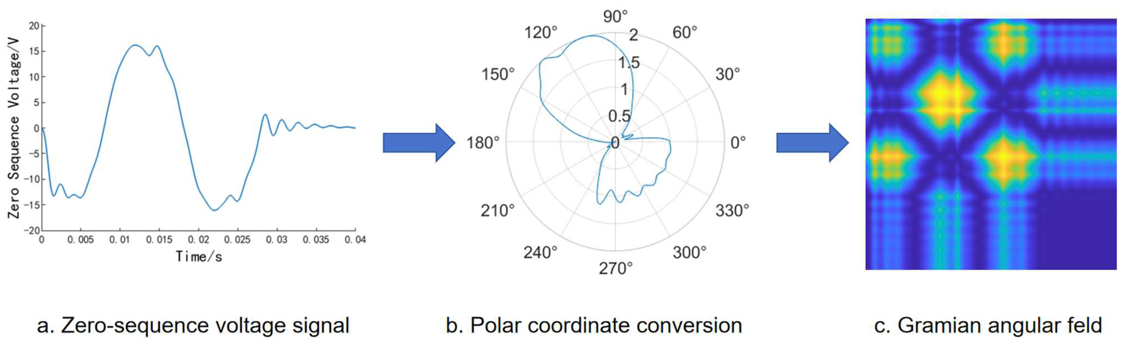
2.1. GAF-Based Time-Series Imaging

The Gramian Angular Field (GAF) is an encoding technique for time-series data. It transforms temporal data into image representations by integrating coordinate transformation and Gramian matrices. The Gramian matrix, constructed from inner products between vectors, effectively preserves temporal dependencies within the time-series. One key limitation of Gramian matrices lies in their inability to distinguish between meaningful signal patterns and Gaussian noise components. To overcome this challenge, we transform the time-series data from Cartesian to polar coordinates before constructing the Gramian matrix representation [31].

Given a time-series $X=(x_t,t=1,2,\dots ,N),$ where t represents the temporal index and $t\in [1,N]$, the Gramian Angular Field transformation proceeds as follows:

• Data Normalization

The symbols and notations used in this paper are listed in the Nomenclature. Following Wang et al. [31], We first normalize the time-series data to the interval [−1, 1] through min–max scaling, which preserves the underlying data distribution. This transformation is expressed as Formula (1):

$${\tilde{x}}_i={\displaystyle \frac{(x_i-\max (X\left)\right)+(x_i-\min (X\left)\right)}{\max (X)-\min (X)}}$$

(1)

where $x_i$ represents the i-th data point in the original time-series, and $X$ represents the complete time-series dataset.

2.

Polar Coordinate Transformation

The data ${\tilde{x}}_i$ obtained from Formula (1) undergoes a polar coordinate transformation to derive the corresponding angle and radius for each data point, with the angle expressed in Formula (2) and the radius in Formula (3):

$${\theta }_i=\arccos ({\tilde{x}}_i),-1\le {\tilde{x}}_i\le 1,{\tilde{x}}_i\in \tilde{X}$$

(2)

$$r_i={\displaystyle \frac{t_i}{M}},t_i\in \mathbb{N}$$

(3)

where $t_i$ represents the position of the data point in the sequence, and $M$ is the normalization factor.

3.

Generation of Gramian Angular Field Image

Using the summation angle relationships presented in Formula (4), we obtain the corresponding Gramian Angular Summation Field (GASF) images:

$$\mathrm{GASF}=\left[\cos \right({\varphi }_i+{\varphi }_j\left)\right] =\widetilde{X^{\prime }}\cdot \tilde{X}-{\sqrt{I-{\tilde{X}}^2}}^{\prime }\cdot \sqrt{I-{\tilde{X}}^2}$$

(4)

where ${\varphi }_i$ and ${\varphi }_j$ represent the angular values at time points i and j, respectively, $\tilde{X}$ denotes the normalized time-series matrix, $\widetilde{X^{\prime }}$ is the transpose of $\tilde{X}$, and $I$ represents the identity matrix.

Figure 2 illustrates the procedure in which Gramian Angular Field transformation converts time-series to images.

2.2. The Crested Porcupine Optimizer (CPO) Algorithm

Inspired by crested porcupine defensive behavior, M. Abdel-Basset et al. [32] developed the CPO. The algorithm features a Cyclic Population Reduction (CPR) technique, reflecting how only threatened individuals activate their defense mechanisms. Following M. Abdel-Basset et al. [32], the mathematical model is expressed in Formula (5):

$$N=N_{\min }+(N^{\prime }-N_{\min })\times (1-({\displaystyle \frac{t\%\frac{T_{\max }}{T}}{\frac{T_{\max }}{T}}}))$$

(5)

where $N$ denotes the current population size, $N^{\prime }$ represents the initial population size, and $N_{\min }$ is the minimum population size required to prevent excessive population reduction. The parameters $t$ and $T_{\max }$ indicate the current and maximum number of iterations, respectively. % represents the remainder or modulo operator. T is a variable to determine the number of cycles.

• Exploration phase

When predators are distant, CPs employ two defensive strategies: visual and acoustic responses. These strategies facilitate broad spatial exploration, focusing on global search capabilities.

(i)

Visual Strategy

As their primary long-range defense, porcupines erect their quills to appear larger and deter predators. This exploration-oriented strategy is mathematically expressed in Formula (6):

$$\overrightarrow{x_i^{t+1}}=\overrightarrow{x_i^t}+{\tau }_1\times \left|2{\tau }_2\times \overrightarrow{x_{best}^t}-\overrightarrow{y_i^t}\right|$$

(6)

where $\overrightarrow{x_i^t}$ denotes the i-th individual position, $\overrightarrow{x_{best}^t}$ represents the global best solution, ${\tau }_1$ and ${\tau }_2$ are step-size control parameters, and $\overrightarrow{y_i^t}$ indicates the candidate solution.

(ii)

Acoustic Strategy

If visual deterrence fails, porcupines escalate their defense by producing threatening sounds. This behavior is mathematically represented as an expansion of the search space through perturbation, as expressed in Formula (7):

$$\overrightarrow{x_i^{t+1}}=(1-\overrightarrow{U_1})\times \overrightarrow{x_i^t}+\overrightarrow{U_1}\times (\overrightarrow{y}+{\tau }_3\times (\overrightarrow{x_{r1}^t}-\overrightarrow{x_{r2}^t}))$$

(7)

where $\overrightarrow{U_1}$ and ${\tau }_3$ are random numbers used to balance the relationship between current and new positions and control the perturbation amplitude, and $\overrightarrow{y}$ represents the target position of the predator after disturbance, while $\overrightarrow{x_{r1}^t}$ and $\overrightarrow{x_{r2}^t}$ denote randomly selected individual positions.

2.

Exploitation phase

In this phase, the CP implements defensive behaviors based on predator proximity, utilizing two strategies: odor attack and physical attack.

(i)

Odor attack strategy

When a predator approaches, the porcupine releases odors to disrupt its movement. In mathematical terms, this strategy involves narrowing the search space to focus on local optima, as shown in Formula (8):

$$\overrightarrow{x_i^{t+1}}=(1-\overrightarrow{U_1})\times \overrightarrow{x_i^t}+\overrightarrow{U_1}\times (\overrightarrow{x_{r1}^t}+S_i^t\times (\overrightarrow{x_{r2}^t}-\overrightarrow{x_{r3}^t})-{\tau }_3\times \overrightarrow{\delta }\times {\gamma }_t\times S_i^t)$$

(8)

where $\overrightarrow{x_{r3}^t}$ denotes the position of a randomly selected individual, $\overrightarrow{\delta }$ is the parameter controlling the search direction, ${\gamma }_t$ represents the defense factor, and $S_i^t$ defines the scent diffusion coefficient.

(ii)

Physical attack strategy

When all else fails, porcupines resort to physical attacks as their last defense. This behavior is mathematically represented by Formula (9):

$$\overrightarrow{x_i^{t+1}}=\overrightarrow{x_{best}^t}+\alpha (1-{\tau }_4)+{\tau }_4\times (\delta \times \overrightarrow{x_{best}^t}-\overrightarrow{x_i^t})-{\tau }_5\times \delta \times {\gamma }_t\times \overrightarrow{F_i^t})$$

(9)

where $\alpha$ is the convergence rate control factor, while ${\tau }_4$ and ${\tau }_5$ are random numbers that control the step size and balance between current and new positions, respectively. $\overrightarrow{F_i^t}$ represents the force acting on the current individual, simulating the predator’s behavioral response after receiving a physical attack.

Compared to traditional optimization algorithms like Particle Swarm Optimization (PSO) and Genetic Algorithms (GAs), the CPO offers several advantages in hyperparameter optimization. While PSO may suffer from premature convergence and GAs can be computationally intensive, the CPO’s Cyclic Population Reduction (CPR) technique provides a better balance between exploration and exploitation. The defense strategies in the CPO—visual, acoustic, odor, and physical attack—enable more effective searching of the parameter space compared to single-strategy algorithms. 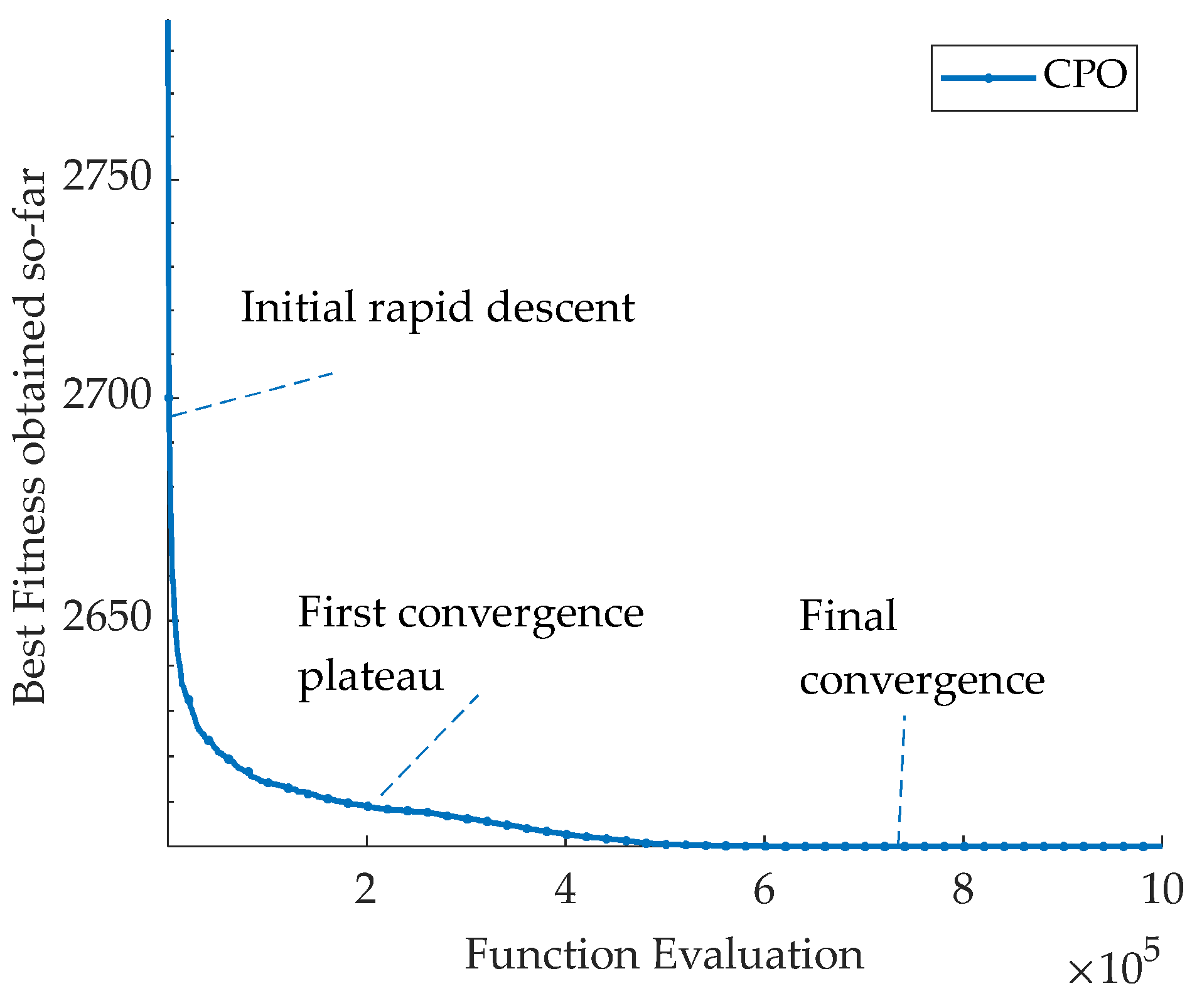Figure 3 shows the evolution of the objective function value during the CPO algorithm optimization process. The following key observations can be drawn:

The algorithm exhibits rapid initial convergence, with the objective function value decreasing sharply. This fast convergence is attributed to the effective global exploration capabilities of visual and sound strategies, allowing the quick identification of promising solution regions. As iterations progress, the convergence curve gradually levels off, indicating the algorithm’s transition to fine-tuning. In this phase, scent and physical attack strategies perform local exploitation, thoroughly exploring promising areas. The convergence curve ultimately stabilizes at a low value, indicating successful identification of near-optimal solutions and algorithm stability. The entire optimization process demonstrates the CPO’s excellent performance through its balanced exploration and exploitation mechanisms.

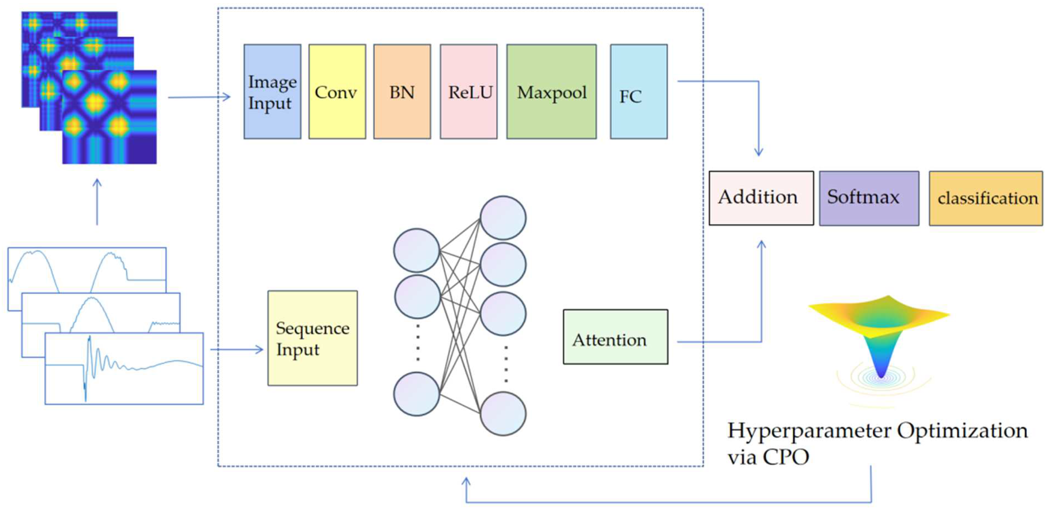
2.3. Dual-Path Neural Networks Optimized by CPO

The proposed framework integrates two core components: a deep learning architecture and an optimization algorithm. Drawing from the dual-channel parallel CNN proposed by Li et al. [33], we designed a dual-path neural network that processes both image and temporal data simultaneously, achieving high-impedance fault identification through feature fusion.

The image processing branch employs a CNN-based structure. It takes 300 × 300 × 3 RGB images as an input with Z-score normalization. A 3 × 3 convolution (stride = 2, padding = 3) is applied, followed by ReLU activation and 3 × 3 max-pooling (stride = 2, padding = 1). The features are then flattened through a 128-neuron fully connected layer. The temporal branch utilizes GRU layers with a self-attention mechanism. Features from both branches are converted to one-dimensional vectors and merged via an addition layer. A three-node fully connected layer processes the fused features before Softmax transformation.

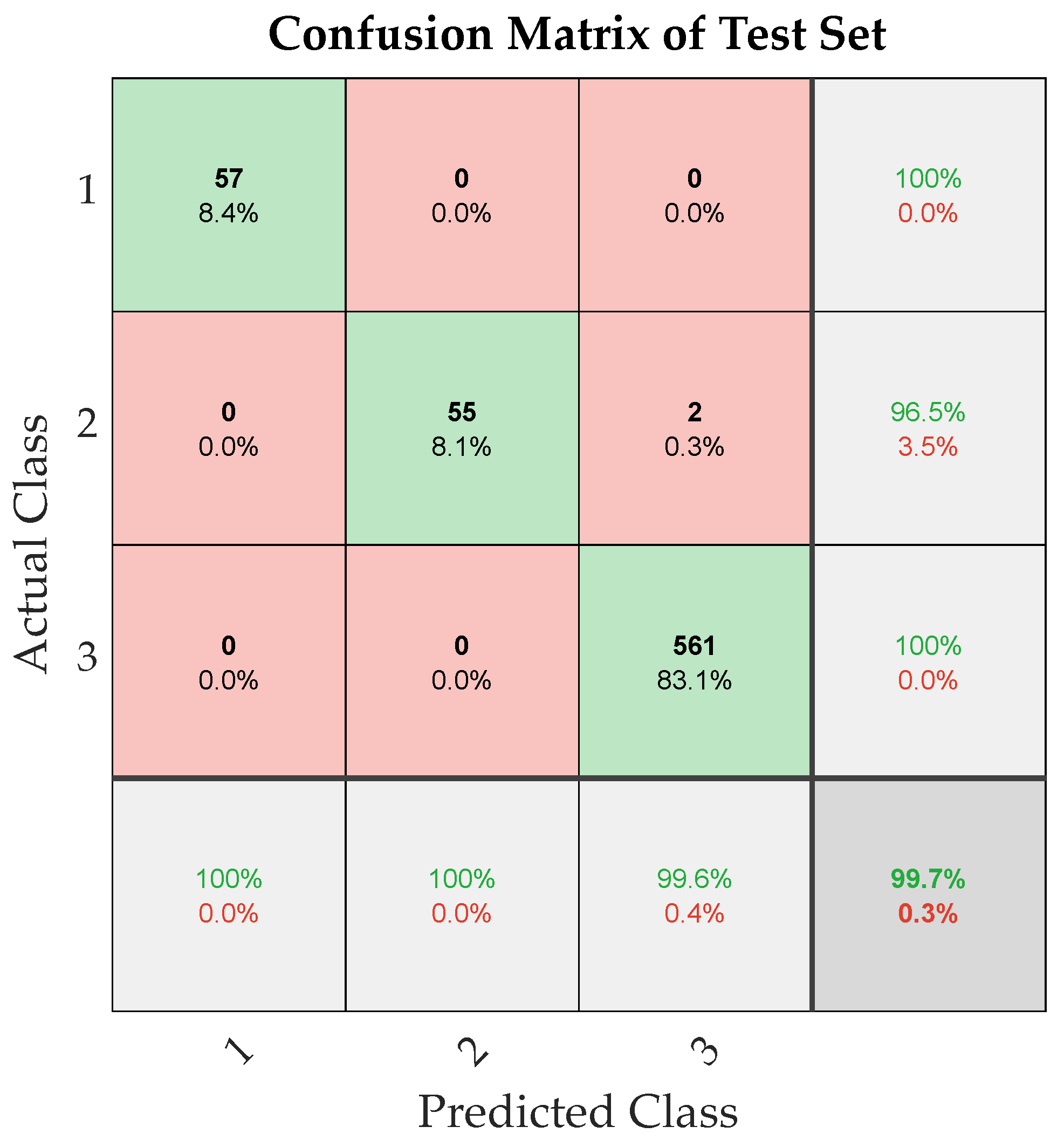
In this study, we employed the CPO to optimize the hyperparameters of the dual-path neural network. The CPO algorithm was initialized with carefully selected parameters based on extensive empirical testing: a population size N′ = 30 with a minimum population size $N_{\min }$ = 24, defense cycle parameter T = 2, convergence rate α = 0.03, and trade-off coefficient T_f = 0.8. These parameters were chosen to balance exploration and exploitation capabilities while maintaining population diversity. The optimization scope encompassed four critical hyperparameters: the learning rate (0.001, 0.01), number of convolution kernels (32, 128), number of GRU neurons(32, 128), and number of attention heads (1, 4). The CPO utilizes four sequential defense mechanisms (sight, sound, odor, and physical attack), while employing Cyclic Population Reduction for efficient convergence and diversity. The algorithm converged to an optimal configuration with 62 convolution kernels, 67 GRU neurons, single-head attention, and a learning rate of 0.0092204. This configuration demonstrated superior performance compared to traditional optimization methods, exhibiting enhanced convergence characteristics and stability. The final model implementation utilized the Adam optimizer with per-epoch data shuffling to mitigate overfitting risks. The CPO-optimized model achieved a remarkable accuracy of 99.7% on the test set, representing a significant improvement over the baseline model’s 98.9% accuracy. Figure 4 illustrates the detailed workflow and structure of our proposed dual-path neural network for high-impedance fault detection.

3. Experimental Setup

3.1. High-Impedance Fault Model

The complex and dynamic characteristics of distribution networks and random factors make accurate HIF modeling challenging. In response, we adopt and extend the nonlinear HIF model proposed by Emanuel et al. [34], which is effective in characterizing nonlinear arcing behavior on sandy soil. By introducing a series resistor to enhance the original model, we better represent the randomness of fault signals, as shown in Figure 5.

The model consists of two DC voltage sources, two diodes, and two resistors. Specifically, $V_p$ and $V_n$ simulate discharge voltages, $R_{\mathrm{p}}$ and $R_n$ represent grounding resistances, and $D_p$ and $D_n$ control fault current directions. Current flows to the ground when the line voltage exceeds $V_p$, reverses when below $V_n$, and ceases when between $V_n$ and $V_p$ due to voltage cancellation [35]. The model parameters are configured with grounding resistance ranging from 500 $\Omega$ to 5000 $\Omega$ and DC voltage sources varying between 3 and 10 kV [36].

3.2. Distribution Network Mode

To validate the proposed method, we constructed a radial medium-voltage distribution network model with an ungrounded neutral point using the MATLAB/SIMULINK R2024a platform, and its topological structure is illustrated in Figure 6.

Table 1. Line parameters.

Type of Line	Parameters	$\mathbf{R}/(\mathbf{\Omega }/\mathbf{k}\mathbf{m})$	$\mathbf{L}/(\mathbf{m}\mathbf{H}/\mathbf{k}\mathbf{m})$	$\mathbf{C}/(\mathsf{\mu }\mathbf{F}/\mathbf{k}\mathbf{m})$
Aerial wire	Positive sequence	0.125	1.3	0.0096
	Zero sequence	0.275	4.6	0.0054
Cable	Positive sequence	0.27	0.255	0.339
	Zero sequence	2.7	1.019	0.28

presents the positive-sequence and zero-sequence parameters of the overhead lines and cable lines in the distribution network model.

3.3. Dataset Construction and Processing

We collected zero-sequence voltage signals from the distribution network model shown in Figure 3 under three scenarios: high-impedance fault, capacitor switching operation, and load connection. For the high-impedance fault samples, we considered varying fault resistances (500–2000 Ω), multiple initial phase angles (0–120°), different fault locations (F1–F5), and all three phases. For the normal operation scenarios, we included capacitor switching with different capacitance values and load connections with varying power levels. By taking samples at different distances from the bus, we obtained a total dataset of 2700 samples. The detailed sample distribution is shown in

Table 2. Distribution of high-impedance fault samples.

Parameter Type	Values
Initial Phase Angle (°)	0, 30, 60, 90, 120
Fault Type	1, 2, 3, 4, 5
Fault Phase	A, B, C
Fault Location	F1, F2, F3, F4, F5
$\mathrm{Neutral} \mathrm{Point} \mathrm{Resistance}/\mathsf{\Omega }$	500, 1000, 2000
$\mathrm{Ground} \mathrm{Resistance}/\mathsf{\Omega }$	5, 10

,

Table 3. Distribution of parameters for capacitor switching samples.

Parameter Type	Values
Initial Phase Angle (°)	0, 30, 60, 90, 120
$\mathrm{Capacitor}/\mathsf{\mu }\mathrm{F}$	0.02, 0.03, 0.04
Switching Phase	A, B, C
Switching Location	F1, F2, F3, F4, F5

and

Table 4. Distribution of parameters for load connection samples.

Parameter Type	Values
Initial Phase Angle (°)	0, 30, 60, 90, 120
$\mathrm{Load}/\mathrm{W}$	150, 200, 250
Switching Phase	A, B, C
Switching Location	F1, F2, F3, F4, F5

.

4. Results and Discussion

4.1. Analysis of Zero-Sequence Voltage Characteristics Under Different Operating Conditions

HIF characteristics often resemble normal operating conditions like load switching and capacitor operations, making fault detection challenging. The significant nonlinearity and instability of HIF signals limit the effectiveness of conventional threshold detection methods based on zero-sequence voltage magnitude, resulting in high false alarm rates.

In distribution networks, when high-impedance faults occur, the high transition resistance results in a minimal or undetectable zero-sequence current, while the zero-sequence voltage exhibits significant variations. Therefore, the zero-sequence voltage serves as a sensitive indicator for identifying such faults. Figure 7, Figure 8 and Figure 9 illustrate the zero-sequence voltage waveforms when a high-impedance ground fault, capacitor switching operation, or load connection occur at t = 0 s, respectively.

Figure 10 presents the two-dimensional feature images obtained through the Gramian Angular Summation Field (GASF) transformation of zero-sequence voltage signals under three operating conditions: high-impedance ground fault, capacitor switching operation, and load connection.

4.2. Model Performance Evaluation and Comparative Analysis

The dataset comprises three types of samples: high-impedance fault, capacitor switching operation, and load connection, split into training and test sets. The model achieved 99.70% accuracy on the test set, demonstrating excellent performance in both fault identification and normal event classification (capacitor switching and load connections). All simulations were performed on a system with Intel(R) Core(TM) i5-10400 CPU @ 2.90 GHz and 16 GB RAM. The model was tested 10 times, and the average testing time per sample was 8.32 ms, making it highly suitable for deployment in large-scale distribution network monitoring systems where real-time performance is crucial.

To demonstrate the effectiveness of feature extraction, we used t-distributed Stochastic Neighbor Embedding (t-SNE) to reduce the high-dimensional features from the fully connected layer to a two-dimensional representation. Figure 11 shows the three event categories (yellow dots, red circles, and blue squares) forming distinct clusters with clear boundaries and tight internal groupings. This visualization confirms the model’s ability to extract discriminative features and effectively differentiate between event types.

Figure 12 shows a radar chart comparing three key performance metrics—Precision, Recall, and F1-score—across all categories. The metrics are plotted on radial axes, where values closer to the perimeter represent better performance. All metrics reach nearly 100%, creating an almost perfect equilateral triangle. This balanced distribution indicates the model’s strong performance in both fault identification and normal condition classification, without compromising either task.

Figure 13 shows the confusion matrix illustrating the model’s classification performance on the test set. In the matrix, rows indicate true classes while columns represent predicted classes, with each cell showing the number of samples in that category. With only two misclassified samples across the entire test set, these results demonstrate the model’s outstanding capability in identifying high-impedance faults.

4.3. Comparative Analysis of Model Performance Under Noisy Conditions

We evaluated our method against three baseline models using the test dataset, as shown in

Table 5. Test accuracy of different models under noise interference (%).

Models	Accuracy Without Noise	Accuracy at 20 dB	Accuracy at 30 dB	Accuracy at 40 dB
Proposed method	99.70	96.74	99.41	99.41
GASF-CNN	99.26	95.70	98.52	98.81
GRU-ATTENTION	97.93	94.37	96.00	97.04
GRU-GASF-CNN	98.81	95.11	97.33	98.80

. Under noise-free conditions, our method achieved 99.70% accuracy, surpassing GASF-CNN (99.26%), GRU-GASF-CNN (98.81%), and GRU-ATTENTION (97.93%) models, demonstrating its effectiveness in identifying high-impedance faults.

To evaluate the model’s resilience to noise, we tested its performance under various noise conditions. We added Gaussian white noise at three SNR levels (20 dB, 30 dB, and 40 dB) to the zero-sequence voltage signals in the test set, with lower SNR values representing stronger noise interference. Our method demonstrated strong noise immunity, achieving accuracies of 96.74%, 99.41%, and 99.41% at 20 dB, 30 dB, and 40 dB, respectively, consistently outperforming the baseline models. These results confirm the model’s robustness in real-world power system environments.

4.4. Model Adaptability Analysis Under Different Topological Configurations

To evaluate the model’s practical applicability and generalization ability, we tested it on a more complex distribution network topology (Figure 14). Considering practical maintenance needs, we simplified the task to binary classification between HIFs and normal operations, as fault detection is the primary concern for maintenance personnel. For validation, we kept the model’s pre-trained parameters unchanged and created a balanced test set by randomly sampling equal numbers of fault and normal operation cases from the new topology. The results show that our model maintains robust performance even under the complex topology, achieving 94% overall accuracy and 96% accuracy in identifying high-impedance faults.

The model’s performance was further evaluated through ROC curve analysis and multiple classification metrics. As shown in Figure 15, the ROC curve demonstrates strong classification performance with an AUC value of 0.940. The curve’s significant deviation from the diagonal line (random classification) indicates the model’s strong discriminative ability.

Figure 16 illustrates the model’s performance metrics for normal operation (Class 1) and high-impedance faults (Class 2). In fault detection, the model achieved 96.0% precision, with the recall, F1-score, and specificity all maintaining values above 90%. These comprehensive metrics demonstrate the model’s robust capability for fault identification in real-world distribution networks.

By contrast, as shown in Figure 17, the single-channel GRU-ATTENTION model shows limited performance, achieving only 89% overall accuracy and 86% accuracy in HIF identification.

The experimental results demonstrate the method’s robustness and accuracy across various network topologies, validating its practical applicability.

4.5. Validation on Real-Time Simulation Platform

We validated the proposed method on the Hardware-in-the-Loop (HIL) experimental platform, as shown in Figure 18. First, we constructed a distribution network model containing five feeders in MATLAB/SIMULINK. In this model, we set up five fault points, labeled as F1 to F5, for fault simulation. Subsequently, using the HIL platform, we performed experiments to collect fault waveform data and imported them into MATLAB for subsequent analysis. To validate the effectiveness of the proposed method, we tested it using 675 samples without retraining the diagnostic model. The fault diagnosis results are shown in

Table 6. Detection results on HIL Platform.

Actual Class	Predicted Class
	HIF	Capacitor Switching	Load Switching
HIF	561	0	0
Capacitor Switching	0	57	0
Load Switching	2	0	55

. As indicated in Table 6, the proposed method only resulted in two misclassifications, demonstrating its robust capability in detecting high-impedance faults on the real-time simulation platform.

5. Conclusions

This paper proposes a dual-path neural network for high-impedance fault detection. The model employs a dual-branch architecture that processes both raw zero-sequence voltage signals and their Gramian Angular Field transformations, effectively combining temporal and spatial features to outperform single-modality methods. The Crested Porcupine Optimizer enhances hyperparameter optimization, improving model adaptability and generalization across various noise levels and network conditions. The Hardware-in-the-Loop validation achieved 99.70% accuracy in distinguishing faults from normal operations, demonstrating the method’s practicality. Future work will focus on reducing computational complexity for real-time applications and extending to more complex networks.

However, the model’s performance under diverse environmental conditions (such as lightning and snow) and its capability to identify emerging load characteristics require further validation. Future research will focus on model generalization in diverse operating environments and the exploration of adaptive optimization strategies for different fault types and network topologies, aiming to enhance the method’s practical value in real distribution networks.

References

1. Allawi, M.N.; Hussain, A.N.; Wali, M.K. A new approach to detecting high impedance fault in power distribution feeder based on signal processing hybrid technique and ANNs. Int. J. Intell. Eng. Syst. 2023, 16. [Google Scholar]
2. Yang, D.; Lu, B.; Lu, H. High-Resistance Grounding Fault Detection and Line Selection in Resonant Grounding Distribution Network. Electronics 2023, 12, 4066. [Google Scholar] [CrossRef]
3. Dashti, R.; Ghasemi, M.; Daisy, M. Fault location in power distribution network with presence of distributed generation resources using impedance based method and applying π line model. Energy 2018, 159, 344–360. [Google Scholar] [CrossRef]
4. Li, B. Technology of fault line selection for single-phase-to-earth fault in small current grounding system. Nonlinear Dyn. 2012, 67, 2111–2122. [Google Scholar] [CrossRef]
5. Baldwin, T.; Renovich, F. Analysis of Fault Locating Signals for High-Impedance Grounded Systems. In Proceedings of the Conference Record of the 2001 IEEE Industry Applications Conference, 36th IAS Annual Meeting (Cat. No.01CH37248), Chicago, IL, USA, 30 September–4 October 2001; Volume 3, pp. 1823–1830. [Google Scholar] [CrossRef]
6. Hu, J.; Wei, L.; McGuire, J.; Liu, Z. Flux linkage detection based ground fault identification and system diagnosis in high-resistance grounding systems. IEEE Trans. Ind. Appl. 2016, 53, 2967–2975. [Google Scholar] [CrossRef]
7. Xu, H.; Zhang, X.; Sun, H.; Wu, W.; Zhu, J.; Wang, F. Faulty section location method for high impedance grounding fault in resonant grounding system based on discrete Fréchet distance. Electr. Power Syst. Res. 2025, 238, 111147. [Google Scholar] [CrossRef]
8. Wang, C.; Feng, L.; Hou, S.; Ren, G.; Lu, T. A High-Impedance Fault Detection Method for Active Distribution Networks Based on Time–Frequency–Space Domain Fusion Features and Hybrid Convolutional Neural Network. Processes 2024, 12, 2712. [Google Scholar] [CrossRef]
9. Chandra, A.; Singh, G.K.; Pant, V. A novel high impedance fault detection strategy for microgrid based on differential energy signal of current signatures and entropy estimation. Electr. Power Compon. Syst. 2024, 52, 532–554. [Google Scholar] [CrossRef]
10. Liu, H.; Zhang, L.; Hang, M.; Li, L. Fault line selection algorithm for single-phase high-impedance ground faults in distribution networks based on the hilbert-huang transform. J. Phys. Conf. Ser. 2024, 2803, 012037. [Google Scholar] [CrossRef]
11. Albanna, E.; Al-Rifaie, A.H.; Al-Karakchi, A.A.A. High impedance fault detection in low voltage overhead distribution based wavelet and harmonic indices. Prz. Elektrotech. 2023, 99, 243–246. [Google Scholar] [CrossRef]
12. Gogula, V.; Edward, B. Advanced signal analysis for high-impedance fault detection in distribution systems: A dynamic Hilbert transform method. Front. Energy Res. 2024, 12, 1365538. [Google Scholar] [CrossRef]
13. Yao, Z.; Liu, Y.; Chen, J.; Ji, J.; Zhang, M.; Gong, Y. Active High-impedance Fault Detection Method for Resonant Grounding Distribution Networks. IEEE Access 2024, 12, 10932–10945. [Google Scholar] [CrossRef]
14. Satea, M.; Elsadd, M.; Zaky, M.; Elgamasy, M. Reliable High Impedance Fault Detection with Experimental Investigation in Distribution Systems. Eng. Technol. Appl. Sci. Res. 2024, 14, 17248–17255. [Google Scholar] [CrossRef]
15. Wang, J.; Zhang, B.; Yin, D.; Ouyang, J. Distribution network fault identification method based on multimodal ResNet with recorded waveform-driven feature extraction. Energy Rep. 2025, 13, 90–104. [Google Scholar] [CrossRef]
16. Lian, Q.; Luo, X.; Lin, D.; Lin, C.; Chen, B.; Guo, Z. ResNest-SVM-based method for identifying single-phase ground faults in active distribution networks. Front. Energy Res. 2024, 12, 1501737. [Google Scholar] [CrossRef]
17. Baharozu, E.; Ihan, S.; Soykan, G. A Data-Driven Based High Impedance Fault Location Method Considering Traveling Waves in Branched Distribution Networks. IEEE Access 2024, 12, 186535–186546. [Google Scholar] [CrossRef]
18. Mohammadi, A.; Jannati, M.; Shams, M. Deep SqueezeNet Based Technique for Detection of High Impedance Arcing Faults in Electric Power Distribution Networks. In Proceedings of the 2024 32nd International Conference on Electrical Engineering (ICEE), Tehran, Iran, 14–16 May 2024; pp. 1–6. [Google Scholar]
19. Jana, C.; Banerjee, S.; Maur, S.; Dalai, S. Power System Disturbance Classification using CWT Guided Customized AlexNet CNN. IEEE Sens. Lett. 2024, 8, 6006204. [Google Scholar] [CrossRef]
20. Zheng, F.; Peng, Y.; Jiang, C.; Lin, Y.; Liang, N. Research on the identification of high-resistance ground faults in the flexible DC distribution network based on VMD–inception–CNN. Front. Energy Res. 2023, 11, 1258619. [Google Scholar] [CrossRef]
21. Zhang, Y.; Wang, X.; Luo, Y.; Zhang, D.; Mirsaeidi, S.; He, J. High Impedance Fault Detection Based on Attention Mechanism and Object Identification. CSEE J. Power Energy Syst. 2021, 10, 197–207. [Google Scholar]
22. Gogula, V.; Edward, B. Fault detection in a distribution network using a combination of a discrete wavelet transform and a neural Network’s radial basis function algorithm to detect high-impedance faults. Front. Energy Res. 2023, 11, 1101049. [Google Scholar] [CrossRef]
23. Guo, M.F.; Guo, Z.Y.; Gao, J.H.; Chen, D.Y. High-impedance fault detection methodology using time–frequency spectrum and transfer convolutional neural network in distribution networks. IEEE Syst. J. 2023, 17, 4002–4013. [Google Scholar] [CrossRef]
24. Liang, H.; Li, H.; Wang, G. A single-phase-to-ground fault detection method based on the ratio fluctuation coefficient of the zero-sequence current and voltage differential in a distribution network. IEEE Access 2023, 11, 7297–7308. [Google Scholar] [CrossRef]
25. Bhatnagar, M.; Yadav, A.; Swetapadma, A.; Abdelaziz, A.Y. LSTM-based low-impedance fault and high-impedance fault detection and classification. Electr. Eng. 2024, 106, 6589–6613. [Google Scholar] [CrossRef]
26. Odion, J.; Ekpa, A.K. Detection and Location of High Impedance Fault on the Nigerian 330 kV Transmission System Using Artificial Neural Network. Int. J. Multidiscip. Res. Anal. 2024, 7, 2092–2101. [Google Scholar]
27. Wu, H.; Wang, J.; Nan, D.; Cui, Q.; Li, W. Fault Location and Fault Cause Identification Method for Transmission Lines Based on Pose Normalized Multi-Output Convolutional Nets. IEEE Trans. Instrum. Meas. 2024, 74, 3500412. [Google Scholar]
28. Ding, C.; Ma, P.; Jiang, C.; Wang, F. Fast Fault Line Selection Technology of Distribution Network Based on MCECA-CloFormer. Appl. Sci. 2024, 14, 8270. [Google Scholar] [CrossRef]
29. Zeng, Z.; Li, J.; Wei, Y.; Wang, X.; Zheng, Y.; Zhang, Y. Flexible DC distribution network fault detection method based on MTF-EfficientNetV2 algorithm. Res. Sq. 2024. [Google Scholar] [CrossRef]
30. Mishra, S.; Giri, N.; Mallick, R.K.; Nayak, P.; Sharma, R.; Gadanayak, D.A. High Impedance Fault Identification Using STransform and 2D-CNN Approach for PV Integrated Micro-grid. In Proceedings of the 2024 IEEE 4th International Conference on Sustainable Energy and Future Electric Transportation (SEFET), Hyderabad, India, 31 July–3 August 2024; pp. 1–5. [Google Scholar]
31. Wang, Z.; Oates, T. Imaging time-series to improve classification and imputation. arXiv 2015, arXiv:1506.00327. [Google Scholar]
32. Abdel-Basset, M.; Mohamed, R.; Abouhawwash, M. Crested Porcupine Optimizer: A new nature-inspired metaheuristic. Knowl.-Based Syst. 2024, 284, 111257. [Google Scholar] [CrossRef]
33. Li, Z.; Chen, Q.; Qian, B.; Niu, Y.; Zhang, Z. Health Diagnosis of Grid-Connected Inverter Switching Devices Based on Gramian Angular Field and Parallel CNN. Electr. Power Autom. Equip. 2024, 44, 153–159. [Google Scholar] [CrossRef]
34. Emanuel, A.E.; Cyganski, D.; Orr, J.A.; Shiller, S.; Gulachenski, E.M. High impedance fault arcing on sandy soil in 15 kV distribution feeders: Contributions to the evaluation of the low frequency spectrum. IEEE Trans. Power Deliv. 1990, 5, 676–686. [Google Scholar] [CrossRef]
35. Gautam, S.; Brahma, S.M. Detection of high impedance fault in power distribution systems using mathematical morphology. IEEE Trans. Power Syst. 2012, 28, 1226–1234. [Google Scholar] [CrossRef]
36. Abasi-obot, I.; Shehu, G.; Kunya, A.; Jibril, Y. High Impedance Fault Modelling and Simulation of 33kV/11kV Distribution Network Using MATLAB. In Proceedings of the 2022 IEEE Nigeria 4th International Conference on Disruptive Technologies for Sustainable Development (NIGERCON), Lagos, Nigeria, 5–7 April 2022; pp. 1–4. [Google Scholar] [CrossRef]
Figure 1. The proposed dual-path neural network for high-impedance fault detection.
Mathematics 13 00225 g001
Figure 2. The procedure for signal–image conversion.
Mathematics 13 00225 g002
Figure 3. Evolution of objective function value in CPO algorithm optimization.
Mathematics 13 00225 g003
Figure 4. Flowchart of proposed dual-path neural network for high-impedance fault detection.
Mathematics 13 00225 g004
Figure 5. Electrical circuit model for high-impedance fault.
Mathematics 13 00225 g005
Figure 6. Topology diagram of distribution network.
Mathematics 13 00225 g006
Figure 7. Zero-sequence voltage under HIF condition.
Mathematics 13 00225 g007
Figure 8. Zero-sequence voltage under capacitor switching.
Mathematics 13 00225 g008
Figure 9. Zero-sequence voltage under load switching.
Mathematics 13 00225 g009
Figure 10. 2D image representations after GASF transformation.
Mathematics 13 00225 g010
Figure 11. The t-SNE visualization of FC layer features.
Mathematics 13 00225 g011
Figure 12. Multi-class performance radar chart.
Mathematics 13 00225 g012
Figure 13. Test set confusion matrix.
Mathematics 13 00225 g013
Figure 14. Complex distribution network topology.
Mathematics 13 00225 g014
Figure 15. ROC curve of model.
Mathematics 13 00225 g015
Figure 16. Binary Classification Performance of the Proposed Model.
Mathematics 13 00225 g016
Figure 17. Classification performance metrics of comparative models.
Mathematics 13 00225 g017
Figure 18. Real-time digital simulator test platform.
Mathematics 13 00225 g018