MeTa Learning-Based Optimization of Unsupervised Domain Adaptation Deep Networks

Abstract

This paper introduces a novel unsupervised domain adaptation (UDA) method, MeTa Discriminative Class-Wise MMD (MCWMMD), which combines meta-learning with a Class-Wise Maximum Mean Discrepancy (MMD) approach to enhance domain adaptation. Traditional MMD methods align overall distributions but struggle with class-wise alignment, reducing feature distinguishability. MCWMMD incorporates a meta-module to dynamically learn a deep kernel for MMD, improving alignment accuracy and model adaptability. This meta-learning technique enhances the model’s ability to generalize across tasks by ensuring domain-invariant and class-discriminative feature representations. Despite the complexity of the method, including the need for meta-module training, it presents a significant advancement in UDA. Future work will explore scalability in diverse real-world scenarios and further optimize the meta-learning framework. MCWMMD offers a promising solution to the persistent challenge of domain adaptation, paving the way for more adaptable and generalizable deep learning models.

1. Introduction

The success of deep learning relies heavily on large annotated datasets. However, annotating a substantial number of images with object content is a time-consuming and labor-intensive task. The advent of Generative Adversarial Networks (GANs) [1] has partially alleviated this issue, facilitating advancements in deep learning by enabling the creation of synthetic data. Despite this progress, existing learning algorithms often struggle with limited generalization across different datasets—a challenge known as domain adaptation (DA). Traditional recognition tasks typically assume that training data (source domain) and testing data (target domain) share a common distribution. In practice, this assumption rarely holds, as test data can come from diverse sources and modalities, leading to poor generalization and the phenomenon known as domain shift.

Various methods have been proposed to tackle domain adaptation [2,3,4,5,6], focusing mainly on aligning feature distributions between domains by measuring and minimizing differences. Another approach in UDA leverages meta-learning to generalize across new, unlabeled domains by learning adaptable representations. For instance, Vettoruzzo et al. [7] proposed a meta-learning framework that optimizes model parameters to achieve effective adaptation across domains with minimal labeled data, showing strong adaptability even with limited unlabeled test samples. This method emphasizes efficient domain adaptation, leveraging knowledge from prior domains to improve generalization under distribution shifts. Recent advancements in deep unsupervised domain adaptation (UDA) have introduced more sophisticated strategies. For instance, a comprehensive 2022 review [8] examined developments such as feature alignment, self-supervision, and representation learning, highlighting current trends and future directions. A 2023 approach employing domain-guided conditional diffusion models [9] demonstrated enhanced transfer performance by generating synthetic samples for the target domain, thus bridging domain gaps more effectively. Additionally, cross-domain contrastive learning [10] has shown promise in promoting domain-invariant features by minimizing feature distances across domains, and manifold-based techniques like Discriminative Manifold Propagation [11] have leveraged probabilistic criteria and metric alignment to achieve both transferability and discriminability.

Domain-Adversarial Neural Networks (DANNs) [4] introduced adversarial training with a gradient reversal layer, laying the groundwork for adversarial domain adaptation approaches. ADDA (Adversarial Discriminative Domain Adaptation) [5] further improved this framework by incorporating untied weight sharing for flexible feature alignment. Deep Adaptation Networks (DANs) [6] employed Maximum Mean Discrepancy (MMD) for kernel-based feature alignment, establishing an influential precedent in UDA. Techniques such as CyCADA [12] combined pixel-level and feature-level adaptations to comprehensively mitigate domain shifts, while MCD (Maximum Classifier Discrepancy) [13] used classifier-based discrepancy maximization to enhance target domain adaptation.

A significant challenge in domain adaptation lies in effectively measuring these distances [2,14]. Classical metrics such as Quadratic [15], Kullback–Leibler [16], and Mahalanobis [17] distances often lack flexibility and fail to generalize across models. Maximum Mean Discrepancy (MMD) [18], which embeds distribution metrics within a Reproducing Kernel Hilbert Space, has gained traction due to its robust theoretical foundation and application in various settings, such as transfer learning [19], kernel Bayesian inference [20], approximate Bayesian computation [21], and MMD GANs [22]. Despite its simplicity, selecting the optimal bandwidth for Gaussian kernels in MMD remains challenging. Liu et al. [23] addressed this by introducing a parameterized deep kernel, known as Maximum Mean Discrepancy with a Deep Kernel (MMDDK), which adapts kernel parameters for more precise domain alignment.

MMD effectively aligns overall domain distributions but struggles with precise class-wise feature alignment. Long et al. [24] addressed this by proposing Class-Wise Maximum Mean Discrepancy (CWMMD), which maps samples from both domains into a shared space and calculates the MMD for each category, summing them to derive the CWMMD. However, these approaches often involve linear transformations, which may not capture complex relationships needed for deeper alignment. Wang et al. [25] provided insights into the MMD’s theoretical foundations, highlighting its role in extracting shared semantic features across diverse categories while maximizing intra-class distances between source and target domains. This approach, however, reduced feature discriminativeness and relied on linear transformations with L2 norm estimations, which may not suffice for general, nonlinear relationships [26,27]. In contrast, deep neural networks, particularly convolutional neural networks (CNNs), excel at learning expressive, nonlinear transformations. Our previous work [28] proposed training a CNN architecture to automatically learn task-specific feature representations.

Meta-learning, or “learning to learn”, has gained attention for its ability to rapidly adapt to new tasks [29,30]. This proposal introduces a novel UDA method that leverages a class-wise, deep kernel-based MMD, optimized through meta-learning. This approach aims to enhance the adaptability and performance of UDA models by incorporating flexible, data-driven kernel learning mechanisms.

The contributions of this paper are summarized as follows: (1) It presents the development of the novel MCWMMD framework, which combines meta-learning with a Class-Wise MMD approach, specifically enhancing class-wise distribution alignment for unsupervised domain adaptation (UDA). (2) It introduces a meta-module that dynamically learns a deep kernel, optimizing domain alignment by adapting to the unique characteristics of each class distribution. (3) It provides a demonstration of improved cross-domain recognition performance, validated through extensive experiments on diverse benchmark datasets, showcasing the framework’s adaptability and effectiveness.

2. Related Work and Key Concepts

This section delves into the foundations and advancements of the Maximum Mean Discrepancy (MMD) metric, a widely used method for measuring the difference between distributions in domain adaptation tasks. We review the evolution of MMD, discussing its theoretical underpinnings, variations, and applications across different models. Additionally, we explore how recent research has extended the MMD to address more complex distributional challenges, including conditional and joint distributions, and we highlight the limitations that these methods seek to overcome. This study considers only two domains for domain adaptation, one source domain and one target domain. $X_s$ and $X_t$ represent the sample sets from the source domain and the target domain, respectively, and $X$ (or $X_{st}$) represents the union of all sample sets in both domains, i.e., $X=X_{st}=X_s\cup X_t$. More symbols and notations are presented in a nomenclature table provided in Table 1.

Table 1. Parameters and variables.

Symbol	Meaning
$X_s$	Set of samples from the source domain.
$X_t$	Set of samples from the target domain.
$X_s^c$	Set of samples of class c from the source domain.
$X_t^c$	Set of samples of class c from the target domain.
$X^c$	Union of source and target samples for class c.
$X$	Union of all samples from source and target domains.
$x_s$	A single sample from the source domain.
$x_t$	A single sample from the target domain.
$Z_s$	Set of feature vectors of samples from the source domain.
$Z_t$	Set of feature vectors of samples from the target domain.
$z_s$	Feature vector of sample $x_s$ from the source domain.
$z_t$	Feature vector of sample $x_t$ from the target domain.
$n_s, n_t$	Number of samples in the source and target domains, respectively.
$n_s^c,n_t^c$	Number of samples of class c in the source and target domains, respectively.
$m_s, m_t$	Mean of samples in the source and target domains, respectively.
$m_s^c,m_t^c$	Mean of samples of class c in the source and target domains, respectively.
$h\left(x\right)$	Deep kernel function mapping features into latent space.
$\Theta$	Set of parameters of the feature extractor network.
$\mathsf{\gamma },\mathsf{\lambda }$	Hyperparameters for balancing loss components.
$\eta$	Learning rate for optimization.

2.1. Domain Adaptation

In machine learning, domain adaptation (DA) is a subfield of transfer learning that focuses on the scenario where there is a significant difference between the data distribution of the training set (source domain) and the test set (target domain). The goal of domain adaptation is to adapt a model trained on the source domain so that it performs well on the target domain despite the differences in data distributions.

The source domain ${\Delta }_s$ is the domain from which we have access to labeled data. Let $X_s={\left\{\left(x_{si}, y_{si}\right)\right\}}_{i=1}^m$ denote the set of $m$ labeled data points from the source domain ${\Delta }_s$, where $x_{si}$ represents the $i$-th data point, and $y_{si}$ is the corresponding label indicating the class to which $x_{si}$ belongs. The label $y_{si}$ belongs to a set of predefined class labels $\mathit{C}=\left\{1,\cdots ,C\right\}$. The target domain ${\Delta }_t$ is the domain to which we want to apply the learned model, but where we only have access to unlabeled data. Let $X_t={\left\{x_{tj}\right\}}_{j=1}^n$ denote the set of $n$ unlabeled data points from the target domain ${\Delta }_t$. Each data point $x_{tj}$ belongs to one of the classes in $\mathit{C}$, but its corresponding label $y_{ti}$ is not observed during training. The source and target domains share a common set of class labels $\mathit{C}=\left\{1,\cdots ,C\right\}$. This implies that, theoretically, the same classes exist in both domains, but the way these classes are represented (i.e., the data distribution) may differ. For instance, the source domain might consist of high-resolution images, while the target domain could consist of lower-resolution images or images taken under different lighting conditions. This distributional difference between the domains poses significant challenges for traditional machine learning models, which typically assume that the training and test data are drawn from the same distribution. To address this challenge, domain adaptation techniques often involve aligning the data distributions between the source and target domains by transforming the feature space or modifying the learning algorithm. One effective method for this is Maximum Mean Discrepancy (MMD), which minimizes the distance between the distributions of the source and target domains in a common latent space. By reducing this distribution shift, MMD helps improve the model’s generalization ability on the target domain, making it a crucial technique for successful domain adaptation.

2.2. RKHS, Kernels, and the Kernel Trick

A Reproducing Kernel Hilbert Space (RKHS) [31] is a powerful mathematical framework widely used in kernel-based learning algorithms. In an RKHS, every function $f$ can be represented as an inner product involving a kernel function $k$, which serves as a measure of similarity between data points. Specifically, for any function $f$ in the RKHS and any point $x$, the value of $f$ at $x$ can be represented as shown in Equation (1), where $⟨·,·{⟩}_H$ denotes the inner product in the RKHS, and $k\left(x,·\right)$ is the kernel function centered at $x$.

$$f\left(x\right)=⟨f, k\left(x,·\right){⟩}_H$$

(1)

The kernel function $k\left(x,y\right)$ implicitly maps data into a high-dimensional feature space, enabling the capture of complex relationships that may not be apparent in the original lower-dimensional space. A widely used kernel is the Gaussian (or RBF) kernel, defined as shown in Equation (2), where $\sigma$ is a parameter that controls the width of the kernel. The Gaussian kernel measures the similarity between two points, $x$ and $y$, based on their distance.

$$k\left(x,y\right)=\exp \left(-{\displaystyle \frac{\Vert x-y_2^2\Vert }{2{\sigma }^2}}\right)$$

(2)

The kernel trick is a crucial technique that enables efficient computation in high-dimensional spaces without explicitly performing mapping. This trick leverages the kernel function to compute the inner product between two points in the feature space $H$ directly in the input space $X$ without needing to know the explicit form of the mapping $\phi \left(·\right)$. For example, let $\phi \left(x\right)$ and $\phi \left(y\right)$ be the mappings of data points $x$ and $y$ into the feature space. The inner product in $x$ and $y$ can be directly evaluated as shown in Equation (3), where $k\left(x,y\right)$ is the kernel function. This means that the product of two elements in the high-dimensional feature space can be evaluated directly in the original input space using the kernel function, such as the Gaussian kernel given in Equation (2).

$$⟨\phi \left(x\right),\phi {\left(y\right)⟩}_H=k\left(x,y\right)$$

(3)

By utilizing the kernel trick, algorithms can efficiently handle nonlinear patterns in the data, making RKHS, kernels, and the kernel trick fundamental components of modern machine learning. This approach simplifies the learning process and reduces computational complexity, enabling operations that would typically require high-dimensional computations to be performed directly in the original input space.

2.3. Maximum Mean Discrepancy (MMD)

Assume that the random samples $X=\left\{x_1,\dots ,x_m\right\}$ and $Y=\left\{y_1,\dots ,y_n\right\}$ come from two probability distributions $\mathrm{P}$ and $\mathrm{Q}$, respectively. The kernel mean embeddings for these distributions are given by ${\mu }_{\mathrm{P}}={\mathbb{E}}_{x\sim \mathrm{P}}\left[\varphi \left(x\right)\right]$ and ${\mu }_{\mathrm{Q}}={\mathbb{E}}_{y\sim \mathrm{Q}}\left[\varphi \left(y\right)\right]$, where the function $\varphi \left(\cdot \right)$ maps the samples into a Reproducing Kernel Hilbert Space (RKHS) $\mathcal{H}$. The Maximum Mean Discrepancy (MMD) [18] between $X$ and $Y$ is defined as the difference between these means in the RKHS, as shown in Equation (4), where $\mathcal{F}$ is the set of functions in the unit ball of the universal RKHS. By squaring the MMD, we can use the kernel trick to compute it directly on the samples with a kernel function $k$ without needing the explicit form of $\varphi \left(\cdot \right)$, as illustrated in Equation (5). The Gaussian kernel shown in Equation (2) is usually used as the kernel function. In practice, for samples $X$ and $Y$, the MMD formula can be adjusted to yield an unbiased estimate, as described in Equation (6).

$$\mathrm{MMD}\left(\mathrm{P},\mathrm{Q}\right)={\parallel {\mu }_{\mathrm{P}}-{\mu }_{\mathrm{Q}}\parallel }_{\mathcal{H}}$$

(4)

$$MM{D}^2\left(\mathrm{P},\mathrm{Q}\right)={⟨{\mu }_{\mathrm{P}}-{\mu }_{\mathrm{Q}}, {\mu }_{\mathrm{P}}-{\mu }_{\mathrm{Q}}⟩}_{\mathcal{H}}={⟨{\mu }_{\mathrm{P}},{\mu }_{\mathrm{P}}⟩}_{\mathcal{H}}+{⟨{\mu }_{\mathrm{Q}},{\mu }_{\mathrm{Q}}⟩}_{\mathcal{H}}-2{⟨{\mu }_{\mathrm{P}},{\mu }_{\mathrm{Q}}⟩}_{\mathcal{H}}={\mathbb{E}}_{x,x^{\prime }\sim \mathrm{P}}\left[k\left(x, x^{\prime }\right)\right]+{\mathbb{E}}_{y,y^{\prime }\sim \mathrm{Q}}\left[k\left(y,y^{\prime }\right)\right]-2{\mathbb{E}}_{x\sim \mathrm{P},y\sim \mathrm{Q}}\left[k\left(x, y\right)\right]$$

(5)

$$MM{D}_u^2\left(X,Y\right)={\displaystyle \frac{1}{m\left(m-1\right)}}{{\displaystyle \sum }}_{i\ne j}^{m}k\left(x_i,x_j\right)+{\displaystyle \frac{1}{n\left(n-1\right)}}{{\displaystyle \sum }}_{\mathrm{i}\ne \mathrm{j}}^{n}k\left(y_i,y_j\right)-{\displaystyle \frac{2}{mn}}{{\displaystyle \sum }}_{i,j}^{m,n}k\left(x_i,y_j\right)$$

(6)

2.4. The Mean Discrepancy with a Deep Kernel

While the Maximum Mean Discrepancy (MMD) defined in a Reproducing Kernel Hilbert Space (RKHS) is a powerful tool for measuring the mean difference between two samples, one of the significant challenges lies in the selection of the bandwidth $\sigma$ for the Gaussian kernel used in the computation. The choice of $\sigma$ is crucial as it directly impacts the sensitivity of the MMD to differences in distributions. However, there is no definitive method for optimally selecting this bandwidth, which can limit the effectiveness of the MMD in practice. To address the issue of bandwidth selection, Liu et al. [23] introduced the Maximum Mean Discrepancy with a Deep Kernel (MMDDK), as described in Equation (7). In this approach, $F_d$ represents a deep neural network that is employed to extract features from the input data. Within this learned feature space, an inner kernel $\kappa$ is applied, typically a Gaussian function with bandwidth ${\sigma }_{\varphi }$, as shown in Equation (8). Additionally, an inner kernel $q$ is applied directly in the input space, also using a Gaussian function but with bandwidth ${\sigma }_q$, as depicted in Equation (9).

The MMDDK framework innovatively combines these kernels by defining a composite kernel function $k_{\omega }\left(x,y\right)$ that integrates both the feature space kernel and the input space kernel. The bandwidth parameters ${\sigma }_{\varphi }$ and ${\sigma }_q$, the weight $ϵ$, and the deep network parameters ${\theta }_d$ are all jointly optimized through a deep learning approach. This joint optimization allows for adaptive bandwidth selection and improved alignment between the source and target distributions.

The entire MMDDK framework is denoted by $F_{\omega }$, where $\omega =\left({\theta }_d, {\sigma }_{\varphi },{\sigma }_q,ϵ\right)$, encapsulating all the parameters involved in the model. The training process aims to maximize an objective function $J_{\lambda }$, as shown in Equation (10), which balances the MMD-based discrepancy measure $MMDD{K}_u^2$ and the variance ${\widehat{\sigma }}_{{ℌ}_1,\lambda }^2$, defined in Equation (11) and Equation (12), respectively. Here, ${ℌ}_1$ refers to the alternative hypothesis in a two-sample test, $\mathrm{P}\ne \mathrm{Q}$, where $\lambda$ is a regularization constant that ensures stability in the optimization process. The function $H_{i,j}$, as defined in Equation (13), calculates the contribution of pairs of samples from both domains, integrating the kernel evaluations across different sample pairs to compute the overall discrepancy. This MMDDK approach addresses the limitations of traditional MMD by allowing for more flexible and adaptive kernel learning, improving the effectiveness of domain adaptation in scenarios where the optimal bandwidth is difficult to determine. The assumption of equal sample sizes in both domains (i.e., $m=n$) simplifies the computations and ensures that the statistical properties of the test remain robust.

$$k_{\omega }\left(x, y\right)=\left[\left(1-ϵ\right)\kappa \left(F_d\left(x\right),F_d\left(y\right)\right)+ϵ\right]q\left(x, y\right)$$

(7)

$$\kappa \left(a,b\right)=\exp \left(-{\displaystyle \frac{{\Vert a-b\Vert }_2^2}{2{\sigma }_{\varphi }^2}}\right)$$

(8)

$$q\left(a, b\right)=\exp \left(-{\displaystyle \frac{{\Vert a-b\Vert }_2^2}{2{\sigma }_q^2}}\right)$$

(9)

$$J_{\lambda }\left(X,Y;k_{\omega }\right)={\displaystyle \frac{MMDD{K}_u^2\left(X,Y;k_{\omega }\right)}{{\widehat{\sigma }}_{{ℌ}_1,\lambda }\left(X,Y;k_{\omega }\right)}}$$

(10)

$$MMDD{K}_u^2\left(X,Y;k_{\omega }\right)={\displaystyle \frac{1}{n\left(n-1\right)}}{{\displaystyle \sum }}_{i\ne j}{H}_{i,j}$$

(11)

$${\widehat{\sigma }}_{{ℌ}_1,\lambda }^2={\displaystyle \frac{4}{n^3}}{{\displaystyle \sum }}_{i=1}^n{\left({{\displaystyle \sum }}_{j=1}^n{H}_{i,j}\right)}^2-{\displaystyle \frac{4}{n^4}}{\left({{\displaystyle \sum }}_{i=1}^n{{\displaystyle \sum }}_{j=1}^n{H}_{i,j}\right)}^2+\lambda$$

(12)

$$H_{i,j}=k_{\omega }\left(x_i,x_j\right)+k_{\omega }\left(y_i,y_j\right)-k_{\omega }\left(x_i,y_j\right)-k_{\omega }\left(y_i,x_j\right)$$

(13)

2.5. Class-Wise Maximum Mean Discrepancy

In domain adaptation, the key challenge arises from the differences between the source and target domains in both marginal and conditional distributions. The marginal distribution captures the overall sample distribution within a domain, while the conditional distribution refers to the distribution of samples within specific classes. Although the Maximum Mean Discrepancy (MMD) is a powerful tool for measuring distributional differences, its common application focuses solely on aligning marginal distributions, often neglecting the alignment of samples with the same labels across domains. This can result in suboptimal performance, particularly when the conditional distributions between the source and target domains differ significantly. To address this issue, Long et al. [24] proposed Joint Distribution Adaptation (JDA), which extends the use of MMD to align both marginal and conditional distributions within a shared linear transformation space. JDA aims to generate feature representations that not only bridge the domain gap but are also robust to significant distributional differences.

In JDA, the source domain samples, $X_s$ $\in R^{d\times n_s}$, and the target domain samples, $X_t\in R^{d\times n_t}$, are mapped onto a common feature space through a linear orthogonal transformation. Here,$n_s$ and $n_t$ denote the number of samples in the source and target domains, respectively, and $d$ is the dimension of the samples. The transformation matrix $A$, which is of size$d\times K$, maps the original data points into a $K$-dimensional feature space. The transformed data points for the source domain are given by $A^T{x}_i$, and similarly, for the target domain by $A^T{x}_j$. The primary objective of this transformation is to minimize the discrepancy between the means of the transformed samples from the source and target domains in this new feature space. The discrepancy is formalized in Equation (14), which represents the MMD they define, where the terms ${\displaystyle \frac{1}{n_s}}{\displaystyle \sum }_{x_i\in X_s}{A}^T{x}_i$ and ${\displaystyle \frac{1}{n_t}}{\displaystyle \sum }_{x_j\in X_t}{A}^T{x}_j$ represent the mean vectors of the transformed data points from the source and target domains, respectively. Their goal is to minimize the Euclidean distance between these two mean vectors, which effectively aligns the marginal distributions of the two domains in the new feature space. On the right side of Equation (14), the trace operation $tr\left(A^T{X}_{st}{M}_0{X}_{st}^{T}A\right)$ is used to express the squared Euclidean distance between the means in a matrix form; the matrix $X_{st}=[X_s|X_t]$ is the concatenated data matrix containing both the source and target samples, resulting in a matrix of size $d\times (n_s+n_t)$; and the matrix $M_0\in R^{n_{st}\times n_{st}}$, defined in Equation (15), is constructed to measure the pairwise relationships between samples in the source and target domains. The elements ${\left(M_0\right)}_{ij}$ define how the relationship between pairs of samples is weighted during the optimization process. When both samples $x_i$ and $x_j$ belong to the source domain ($x_i,x_j\in X_s$), the element ${\left(M_0\right)}_{ij}$ is assigned a positive weight ${\displaystyle \frac{1}{n_s{n}_s}}$. Similarly, when both samples belong to the target domain ($x_i,x_j\in X_t$), the weight is ${\displaystyle \frac{1}{n_t{n}_t}}$. These positive weights contribute to aligning the means of the samples within each domain. For pairs where one sample is from the source domain and the other from the target domain, ${\left(M_0\right)}_{ij}$ is assigned a negative weight ${\displaystyle \frac{-1}{n_s{n}_t}}$. These negative weights are crucial for minimizing the discrepancy between the source and target domain means by penalizing large differences between them. The matrix $M_0$ plays a pivotal role in the optimization objective by guiding the linear transformation $A$ to map the source and target samples into a common feature space where their distributions are aligned. The trace operation in Equation (14) sums the weighted differences across all pairs of samples, driving the minimization process towards the optimal alignment of both marginal and conditional distributions. The JDA method, through the use of the linear transformation matrix $A$ and the carefully constructed matrix $M_0$, effectively addresses the limitations of traditional MMD by jointly aligning both marginal and conditional distributions. This joint alignment is crucial for improving the performance of domain adaptation tasks, particularly in scenarios where the source and target domains exhibit significant distributional differences. The mathematical framework provided by Equations (14) and (15) ensures that the adaptation process considers the complex relationships between the source and target domains, leading to more robust and generalizable models.

$$MM{D}^2=\left|\right|{\displaystyle \frac{1}{n_s}}{{\displaystyle \sum }}_{x_i\in X_s}{A}^T{x}_i-{\displaystyle \frac{1}{n_t}}{{\displaystyle \sum }}_{x_j\in X_t}{A}^T{x}_j|{|}_2^2=tr\left(A^T{X}_{st}{M}_0{X}_{st}^{T}A\right)$$

(14)

$${\left(M_0\right)}_{ij}=\left\{\begin{array}{cc}{\displaystyle \frac{1}{n_s{n}_s}},& x_i,x_j\in X_s\\ {\displaystyle \frac{1}{n_t{n}_t}},& x_i,x_j\in X_t\\ {\displaystyle \frac{-1}{n_s{n}_t}},& otherwise\end{array}\right.$$

(15)

The challenge of matching conditional distributions (i.e., distributions conditioned on class labels) arises from the difficulty of doing so without labeled data in the target domain. To address this, Long et al. [24] proposed using pseudo labels for the target samples. These pseudo labels can be inferred by applying classifiers trained on the labeled source data to the unlabeled target data. This allows for the approximation of class-conditional distributions in the target domain, enabling the calculation of the discrepancy between class-conditional distributions in the source and target domains. To quantify this discrepancy, Long et al. introduced the Class-Wise Maximum Mean Discrepancy (CWMMD), which modifies the standard MMD to focus on class-conditional distributions. The formulation of CWMMD is given in Equation (16), where $X_s^c$ and $X_t^c$ represent the data samples belonging to the c-th class from the source and target domains, respectively; $n_s^c$ and $n_s^c$ are the numbers of samples in the c-th class for the source and target domains, respectively; and $A$ is a projection matrix that maps the data into a common subspace where the distributions are compared. The term on the left-hand side of Equation (16) represents the squared Euclidean distance between the class-conditional distributions of the source and target domains after projection by $A$. The right-hand side expresses this same discrepancy in its matrix trace form, where $X_{st}=\left[X_s,X_t\right]$ denotes the combined source and target data and $M_c$ is a class-specific matrix that encodes the relationships between pairs of samples from the source and target domains within the same class, as defined in Equation (17).

$$CWMM{D}^2={{\displaystyle \sum }}_{c=1}^C\left|\right|{\displaystyle \frac{1}{n_s^c}}{{\displaystyle \sum }}_{x_i\in X_s^c}{A}^T{x}_i-{\displaystyle \frac{1}{n_t^c}}{{\displaystyle \sum }}_{x_j\in X_t^c}{A}^T{x}_j|{|}_2^2={{\displaystyle \sum }}_{c=1}^{C}tr\left(A^T{X}_{st}{M}_c{X}_{st}^{T}A\right)$$

(16)

$${\left(M_c\right)}_{ij}=\left\{\begin{array}{c}\begin{array}{c}{\displaystyle \frac{1}{n_s^c{n}_s^c}}, x_i,x_j\in X_s^c \\ {\displaystyle \frac{1}{n_t^c{n}_t^c}}, x_i,x_j\in X_t^c \end{array} \\ \begin{array}{c}{\displaystyle \frac{-1}{n_s^c{n}_t^c}}, \left\{\begin{array}{c}{x}_i\in X_s^c,x_j\in X_t^c\\ x_j\in X_s^c,x_i\in X_t^c\end{array}\right. \\ 0, \mathrm{otherwise} \end{array}\end{array}\right.$$

(17)

To achieve effective transfer learning, Long et al. proposed the Joint Distribution Adaptation (JDA) framework, which combines the marginal MMD (addressed in Equation (14) with the class-conditional CWMMD addressed in Equation (16). The resulting optimization problem is shown in Equation (18), where ${{\displaystyle \sum }}_{c=0}^{C}tr\left(A^T{X}_{st}{M}_c{X}_{st}^{T}A\right)$ combines the marginal and conditional discrepancies into a single objective, where $c=0$ corresponds to the marginal distribution, $\alpha {\Vert A\Vert }_F^2$ is a regularization term that controls the scale of the projection matrix $A$, ensuring the problem is well posed and prevents overfitting, and the constraint $A^T{X}_{st}{H}_{st}{X}_{st}^{T}A=I_{K\times K}$ restricts the total variation in the projected data to a fixed value, preserving important statistical information. Here, $H_{st}=I_{n_{st}\times n_{st}}-{\displaystyle \frac{1}{n_{st}}}{\mathbf{1}}_{n_{st}\times n_{st}}$ is a centering matrix that ensures the projected data are centered, with $n_{st}^c=n_s^c+n_s^c$ representing the total number of samples. This optimization problem is designed to find the optimal projection matrix $A$ that aligns both marginal and conditional distributions across domains, thereby enabling effective domain adaptation even when the target domain lacks labeled data.

$$\underset{A}{\min }{{\displaystyle \sum }}_{c=0}^{C}tr\left(A^T{X}_{st}{M}_c{X}_{st}^{T}A\right)+\alpha {\Vert A\Vert }_F^2 s.t. A^T{X}_{st}{H}_{st}{X}_{st}^{T}A=I_{K\times K}$$

(18)

2.6. Discriminative Class-Wise MMD Based on Euclidean Distance

The use of MMD aims to extract shared common features between the source and target domains by minimizing the mean difference for each pair of classes, even when their distributions are distinct. How is this achieved in practice? Wang et al. [25] provided valuable insights, illustrating that the principles of MMD closely mirror human transferable learning behaviors. Their approach treats each category as a distinct group, analyzing and adjusting the means of specific categories in both the source and target domains. For example, in the case of a specific class shared by the source and target domains, the category means are progressively aligned by minimizing the mean difference between the pairs, maximizing their intra-class distances. As the domain adaptation (DA) process progresses, the means of these classes from the two domains converge, reducing joint variance and improving feature alignment. This process reflects how humans naturally extract shared features from underlying semantics, capturing broad patterns while forgoing some finer details. The progressive alignment of category means exemplifies how MMD enhances feature generalization across domains, facilitating robust domain adaptation.

Wang et al. [25] presented Lemmas 1–3 as follows, where Lemmas 2 and 3 were both proven by them, and Lemma 1 follows the identity about the inter-class (or between-class) distance according to [32]:

Lemma 1.

The inter-class scatter $S_b$ is defined as the squared inter-class distance and can be expressed as

$$S_b=tr\left(A^T{\mathit{S}}_{b}A\right)={\displaystyle \frac{1}{n}}{{\displaystyle \sum }}_{c=1}^C{{\displaystyle \sum }}_{k=c+1}^C{n}^c{n}^{k}tr\left(A^T{D}^{ck}A\right),$$

(19)

where $D^{ij}=\left({\mathit{m}}^i-{\mathit{m}}^j\right){\left({\mathit{m}}^i-{\mathit{m}}^j\right)}^T$, ${\mathit{S}}_b={\displaystyle \sum }_{i=1}^C{n}^i\left({\mathit{m}}^i-\mathit{m}\right){\left({\mathit{m}}^i-\mathit{m}\right)}^T$ is the inter-class scatter matrix, $n^i$ is the number of data instances in the i-th category, ${\mathit{m}}^i$ represents the mean of data samples from the $i$-th category, and $\mathit{m}$ represents the mean of the whole data samples. For brevity, we omit the proofs.

Lemma 2.

The squared inter-class distance equals to the data variance minus the squared intra-class distance:

$$S_b=S_v-S_w,$$

(20)

where $S_v=tr\left(A^T{\mathit{S}}_{v}A\right)$ is the variance, $S_w=tr\left(A^T{\mathit{S}}_{w}A\right)$ is the squared intra-class (or within-class) distance, ${\mathit{S}}_v={{\displaystyle \sum }}_{i=1}^n\left({\mathit{x}}_i-\mathit{m}\right){\left({\mathit{x}}_i-\mathit{m}\right)}^T$, and ${\mathit{S}}_w={{\displaystyle \sum }}_{c=1}^C{{\displaystyle \sum }}_{x_j\in X^c}\left({\mathit{x}}_j-\mathit{m}\right){\left({\mathit{x}}_j-\mathit{m}\right)}^T$.

Lemma 3.

The following identity describes the Class-Wise Maximum Mean Discrepancy (CWMMD):

$$CWMMD={{\displaystyle \sum }}_{c=1}^{C}tr\left(A^{T}X{M}_c{X}^{T}A\right)={{\displaystyle \sum }}_{c=1}^C{\displaystyle \frac{n_s^c+n_t^c}{n_s^c{n}_t^c}}tr\left(A^T{\left({\mathit{S}}_{st}\right)}_b^{c}A\right)={{\displaystyle \sum }}_{c=1}^C{\displaystyle \frac{n_s^c+n_t^c}{n_s^c{n}_t^c}}tr\left(A^T{\left({\mathit{S}}_{st}\right)}_v^{c}A\right)-{{\displaystyle \sum }}_{c=1}^C{\displaystyle \frac{n_s^c+n_t^c}{n_s^c{n}_t^c}}tr\left(A^T{\left({\mathit{S}}_{st}\right)}_w^{c}A\right),$$

(21)

where

$${\left({\mathit{S}}_{st}\right)}_b^c={{\displaystyle \sum }}_{i\in \left\{s, t\right\}}{n}_i^c\left({\mathit{m}}_i^c-{\mathit{m}}_{st}^c\right){\left({\mathit{m}}_i^c-{\mathit{m}}_{st}^c\right)}^T,$$

(22)

$${\left({\mathit{S}}_{st}\right)}_v^c={{\displaystyle \sum }}_{i=1}^{n_{st}^c}\left({\mathit{x}}_i-{\mathit{m}}_{st}^c\right){\left({\mathit{x}}_i-{\mathit{m}}_{st}^c\right)}^T,$$

(23)

and

$${\left({\mathit{S}}_{st}\right)}_w^c={{\displaystyle \sum }}_{i\in \left\{s, t\right\}}{{\displaystyle \sum }}_{j=1}^{n_i^c}\left({\mathit{x}}_j-{\mathit{m}}_i^c\right){\left({\mathit{x}}_j-{\mathit{m}}_i^c\right)}^T.$$

(24)

where $n_i^c$ denotes the number of data instances in the  $c$-th category from domain i (where i can be either source s or target t), and $n_{st}^c=n_s^c+n_t^c$. Additionally, ${\mathit{m}}_i^c$ represents the mean of data in the $c$-th category from domain $i$, while ${\mathit{m}}_{st}^c$ denotes the mean of data in the $c$-th category from both the source and target domains combined. The subscription st of ${\mathit{S}}_{st}$ signifies that both the source and target domains are considered together.

Notably, in this paper, we correct a statement proposed by Wang et al. The original statement, “The inter-class distance equals the data variance minus the intra-class distance”, should be revised to “The squared inter-class distance equals the data variance minus the squared intra-class distance”.

Let $S_b^c$= $tr\left(A^T{X}_{st}{M}_c{X}_{st}^{T}A\right)$ be the squared inter-class distance in the transformed space based on transformation matrix $A$ for class $c$ between the source and target domains. Then, let $S_b={{\displaystyle \sum }}_{c=1}^C{S}_b^c$ so that Equation (18) can be written as Equation (25). According to the identity, $S_b=S_v-S_w$, derived by Wang et al. [25], Equation (25) can be written as Equation (26), where $S_w$ is the squared intra-class distance between the source and target domains, and $S_v$ is their variance. Therefore, minimizing the squared inter-class distance $S_b$ is equivalent to maximizing the squared intra-class distance $S_w$ while simultaneously minimizing their variance $S_v$, thereby reducing feature distinguishability. To propose a solution, a balance parameter $\beta \left(-1\le \beta \le 1\right)$ is directly applied to the hidden squared intra-class distance in $S_w$ to regulate its variation, as shown in Equation (27).

$$\underset{A}{\min }\left(S_b+MM{D}^2+\alpha {\Vert A\Vert }_F^2\right) s.t. A^T{X}_{st}{H}_{st}{X}_{st}^{T}A=I_{k\times k}$$

(25)

$$\underset{A}{\min }\left(S_v-S_w+MM{D}^2+\alpha {\Vert A\Vert }_F^2\right) s.t. A^T{X}_{st}{H}_{st}{X}_{st}^{T}A=I_{k\times k}$$

(26)

$$\underset{A}{\min }\left(S_v+\beta ·S_w+MM{D}^2+\alpha {\Vert A\Vert }_F^2\right) s.t. A^T{X}_{st}{H}_{st}{X}_{st}^{T}A=I_{k\times k}$$

(27)

2.7. Discriminative Class-Wise MMD Based on Gaussian Kernels

Wang et al. [25] extended the work of Long et al. [24] by introducing a discriminative Class-Wise MMD, which retains the use of linear transformations to project samples into the feature space and employs the Euclidean distance to measure the mean difference between the distributions of samples from two domains. However, linear transformations are generally less effective and efficient compared to nonlinear transformations, such as those applied in the Reproducing Kernel Hilbert Space (RKHS), where more complex patterns and relationships between domains can be captured.

In our previous research [28], we redefined the MMD proposed by Wang et al. by incorporating a Gaussian kernel within the RKHS framework, as RKHS based on the Gaussian kernel is universal [33]. This modification enables the MMD to be computed more efficiently and flexibly using the kernel trick, enhancing its applicability to a broader range of scenarios. Firstly, we redefined the squared inter-class distance $S_b$, the squared intra-class distance $S_w$, and the variance $S_v$ as $S_{inter}$,$S_{intra}$, and $S_{var}$, respectively, in Definitions 1 through 3. We then proved that under the Gaussian kernel MMD, the MMD representing the inter-class distance between the source and target domains can be decomposed into the intra-class distance and variance within the source and target domains.

Definition 1.

The squared inter-class distance between the source and target domains is defined as $S_{inter}={{\displaystyle \sum }}_{c=1}^C{\left(S_{st}\right)}_{inter}^c$, where ${\left(S_{st}\right)}_{inter}^c$ is the squared inter-class distance for class c between the source and target domains, as shown in Equation (28).

$${\left(S_{st}\right)}_{inter}^c={\displaystyle \frac{1}{{\left(n_s^c\right)}^2}}{{\displaystyle \sum }}_{x_i,x_j\in X_s^c}{⟨x_i,x_j⟩}_{\mathcal{H}}+{\displaystyle \frac{1}{{\left(n_t^c\right)}^2}}{{\displaystyle \sum }}_{x_i,x_j\in X_t^c}{⟨x_i,x_j⟩}_{\mathcal{H}}-{\displaystyle \frac{2}{n_s^c{n}_t^c}}{{\displaystyle \sum }}_{x_i\in X_s^c,x_j\in X_t^c}{⟨x_i,x_j⟩}_{\mathcal{H}}$$

(28)

Definition 2.

The squared intra-class distance between the source and target domains is defined as $S_{intra}={{\displaystyle \sum }}_{c=1}^C{\left(S_{st}\right)}_{intra}^c$, where ${\left(S_{st}\right)}_{intra}^c$ is the squared intra-class distance for class c between the source and target domains, as shown in Equation (29).

$${\left(S_{st}\right)}_{intra}^c={\displaystyle \frac{n_s^c+n_t^c}{n_s^c{n}_t^c}}\left[{{\displaystyle \sum }}_{x_i\in X_{st}^c}{⟨x_i,x_i⟩}_{\mathcal{H}}-{\displaystyle \frac{1}{n_s^c}}{{\displaystyle \sum }}_{x_i,x_j\in X_s^c}{⟨x_i,x_j⟩}_{\mathcal{H}}-{\displaystyle \frac{1}{n_t^c}}{{\displaystyle \sum }}_{x_i,x_j\in X_t^c}{⟨x_i,x_j⟩}_{\mathcal{H}}\right]$$

(29)

Definition 3.

The variance between the source and target domains is defined as $S_{var}={{\displaystyle \sum }}_{c=1}^C{\left(S_{st}\right)}_{var}^c$, where ${\left(S_{st}\right)}_{var}^c$ is the total variance for class c between the source and target domains, as shown in Equation (30).

$${\left(S_{st}\right)}_{var}^c={\displaystyle \frac{n_s^c+n_t^c}{n_s^c{n}_t^c}}{{\displaystyle \sum }}_{x_j\in X_{st}^c}{⟨x_j,x_j⟩}_{\mathcal{H}}-{\displaystyle \frac{1}{n_s^c{n}_t^c}}{{\displaystyle \sum }}_{x_i,x_j\in X_s^c}{⟨x_i,x_j⟩}_{\mathcal{H}}-{\displaystyle \frac{1}{n_s^c{n}_t^c}}{{\displaystyle \sum }}_{x_i,x_j\in X_t^c}{⟨x_i,x_j⟩}_{\mathcal{H}}-{\displaystyle \frac{2}{n_s^c{n}_t^c}}{{\displaystyle \sum }}_{x_i\in X_s^c,x_j\in X_t^c}{⟨x_i,x_j⟩}_{\mathcal{H}}$$

(30)

Theorem 1.

$S_{inter}=S_{var}-S_{intra}$.

Our previous work [28] established Theorem 1 and provided proof. Traditional MMD, without categorization, is the inter-class distance of samples from the two domains, referred to as marginal MMD, defined in Equation (31). Class-Wise MMD refers to the inter-class distance of samples from specific categories in the two domains, termed conditional MMD. For example, ${\left(S\right)}_{inter}^c$ is the squared MMD or the squared inter-class distance for class c between the two domains and can be defined as $MM{D}_c^2={\left(S\right)}_{inter}^c$. As a result, the loss function $L_{cwmmd}$ based on Class-Wise Maximum Mean Discrepancy is defined as the sum of and the squared inter-class distance $S_{inter}$ and the squared marginal MMD, as shown in Equation (32), which can also be written as Equation (33) according to Theorem 1. To address the reduction in feature discriminability, we adopt the strategy proposed by Wang et al. [25], introducing a balance parameter $\beta \left(-1\le \beta \le 1\right)$ to the hidden squared intra-class distance within the squared inter-class distance $S_{inter}$. This modification adjusts the loss function, resulting in $L_{dcwmmd}$, as shown in Equation (34).

$$MM{D}^2\left(X_s,X_t\right)={\displaystyle \frac{1}{{\left(n_s\right)}^2}}{{\displaystyle \sum }}_{x_i\in X_s}{{\displaystyle \sum }}_{x_j\in X_s}{⟨x_i,x_j⟩}_{\mathcal{H}}+{\displaystyle \frac{1}{{\left(n_t\right)}^2}}{{\displaystyle \sum }}_{x_i\in X_t}{{\displaystyle \sum }}_{x_j\in X_t}{⟨x_i,x_j⟩}_{\mathcal{H}}-{\displaystyle \frac{2}{n_s{n}_t}}{{\displaystyle \sum }}_{x_i\in X_s}{{\displaystyle \sum }}_{x_j\in X_t}{⟨x_i,x_j⟩}_{\mathcal{H}}$$

(31)

$$L_{cwmmd}=S_{inter}+MM{D}^2\left(X_s,X_t\right)$$

(32)

$$L_{cwmmd}=S_{var}-S_{intra}+MM{D}^2\left(X_s,X_t\right)$$

(33)

$$L_{dcwmmd}=S_{var}+\beta ·S_{intra}+MM{D}^2\left(X_s,X_t\right)$$

(34)

3. The Proposed Method

The proposed unsupervised domain adaptation (UDA) approach primarily utilizes Discriminative Class-Wise Maximum Mean Discrepancy (MMD) to align the class-level data distributions of the source and target domains, which addresses the issue of reduced feature distinguishability when MMD minimizes the mean deviation between two different domains, thereby effectively achieving the goal of UDA. However, the MMD used here is learned with a meta-module MTMMD to obtain MMD with deep kernels (MMDDK). The framework of the proposed method is directly called MeTa Discriminative Class-Wise MMD (MCWMMD), as shown in Figure 1. The orange block represents the feature extractor F, which is responsible for extracting domain-invariant features. The green block represents the classifier C, which predicts class labels based on the extracted features. The light red block represents the meta-module MTMMD, referred to as “MMDDK”, which is designed to measure the distance between feature distributions of samples from the two domains.

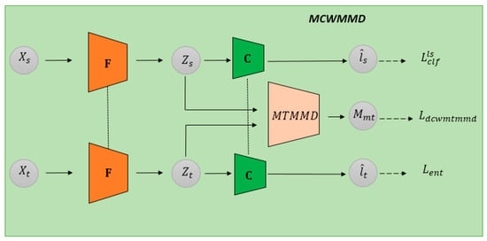
Figure 1. Training framework for MCWMMD.

The training objective of the meta-module MTMMD is to enhance its ability to discriminate between the two domains. This is achieved by updating MMDDK to maximize the feature distance measurement values of samples from the two domains. Conversely, the training objective of the MCWMMD module is to update the feature extractor F so that the feature distance measurement values of samples from the two domains, computed using the current MTMMD, are minimized.

These opposing training objectives result in a process resembling adversarial training, where the two modules iteratively adjust to counteract each other. This alternating training process allows each module to improve its performance while balancing the influence of the other. The remainder of this section will introduce the detailed training processes of these two modules.

3.1. Deep Kernel Training Network

According to the Maximum Mean Discrepancy with Deep Kernels (MMDDK) defined by Liu et al. [23], as explained in Equation (7), we construct a training network for MMDDK, as depicted in Figure 2. The input to the training network for MMDDK is the feature vector $z=F\left(x\right)$ extracted from the MCWMMD network, where two vectors, $z_s=F\left(x_s\right)$ and $z_t=F\left(x_t\right)$ (referred to as first-order features), are used to compute the Gaussian function value $q\left(z_s, z_t\right)$ in Equation (9). Additionally, they are separately input into another feature extractor $F_d$ to obtain ${\widehat{z}}_s=F_d\left(z_s\right)$ and ${\widehat{z}}_t=F_d\left(z_t\right)$ (referred to as second-order features), which are used to compute the Gaussian function value $\kappa \left({\widehat{z}}_s,{\widehat{z}}_t\right)$ in Equation (8). Subsequently, the two Gaussian function values $q\left(z_s, z_t\right)$ and $\kappa \left({\widehat{z}}_s,{\widehat{z}}_t\right)$ are combined using the operator $k_{\omega }$ defined in Equation (7) to calculate the deep kernel distance $k_{\omega }\left(z_s, z_t\right)$. The parameters ${\sigma }_{\varphi }$,${\sigma }_q$, weight $ϵ$, and network parameters ${\theta }_d$ of the network $F_d$ are jointly trained using this deep neural network, denoted as $F_{\omega }$, where $\omega =\left({\theta }_d, {\sigma }_{\varphi },{\sigma }_q,ϵ\right)$. Its training is based on maximizing the objective function $J_{\lambda }$ in Equation (10). The network training algorithm is presented in Algorithm 1.

Algorithm 1 Training the MMDDK
Input: ${\eta }_1$; Initialize $\omega \leftarrow ({\theta }_d,$ ${\sigma }_{\varphi },$ ${\sigma }_q,$ $ϵ)$; repeat until convergence   $\left(X_s,Y_s\right)=\left\{\left(x_{s1},y_{s1}\right),\left(x_{s2},y_{s2}\right),\dots ,\left(x_{sN},y_{sN}\right)\right\}\leftarrow$mini-batch from ${\Delta }_s$;   $X_t=\left\{x_{t1},x_{t2},\dots ,x_{tN}\right\}\leftarrow$mini-batch from ${\Delta }_t$;   $Z_s\leftarrow F\left(X_s\right);Z_t\leftarrow F\left(X_t\right);$   ${\widehat{Z}}_s\leftarrow F_d\left(Z_s\right);{\widehat{Z}}_t\leftarrow F_d\left(Z_t\right);$
$M\left(\mathsf{\omega }\right)\leftarrow MMDD{K}_u^2\left(Z_s,Z_t;k_{\omega }\right)$;	#using (11)
$V\left(\mathsf{\omega }\right)\leftarrow {\sigma }^2\left(Z_s,Z_t;k_{\omega }\right)$;	#using (12) with $\mathsf{\lambda }=0$
$J\left(\mathsf{\omega }\right)\leftarrow M\left(\mathsf{\omega }\right)$/$\sqrt{V\left(\mathsf{\omega }\right)}$ ;	#using (10)
#update parameters:
$\omega \leftarrow \omega +{\eta }_1{\nabla }_{\omega }J\left(\mathsf{\omega }\right)$;	#maximizing J
end repeat

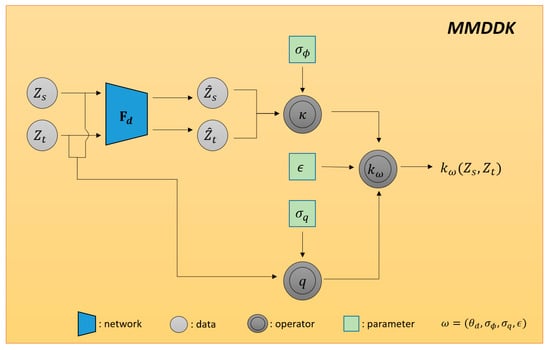
Figure 2. Training framework for MMDDK.

3.2. Meta-Learning of Maximum Mean Discrepancy

In this section, we redefine and compute the Maximum Mean Discrepancy (MMD) originally defined and calculated by Wang et al. [25] in the context of linear transformation spaces, but now in the Reproducing Kernel Hilbert Space (RKHS) using the kernel trick for straightforward MMD computation. Consequently, we also redefine their definitions of between-class distance squared ($S_{inter}$), within-class distance squared ($S_{intra}$), and variance ($S_{var}$), and demonstrate that under the Gaussian kernel-based MMD, the between-class distance-squared MMD between the source and target domains can be decomposed into the sum of within-class distance-squared MMDs from both domains and their variance difference.

As described in Section 2, minimizing the between-class distance squared $S_{inter}$ is equivalent to maximizing the within-class distance squared $S_{intra}$ for both the source and target domains while simultaneously minimizing their total variance $S_{var}$, which leads to decreased feature discriminability. To address this issue, a balancing parameter $\beta$ ($-1\le \beta \le 1$) is applied to the hidden within-class distance squared $S_{intra}$ within $S_{inter}$, proposing the discriminability class-level loss function $L_{dcwmmd}$ defined in Equation (34), which can be rewritten as Equation (35).

For convenience, let us define $MM{D}_0={\left(S_{st}\right)}_{inter}^0=MMD$. Hence, Equation (35) can also be rewritten as Equation (36), where the second term represents the sum of marginal MMD and conditional MMD, and the coefficient ${\beta }^{\prime }=\beta +1$ adjusts between 0 and 2, i.e., 0 $\le \beta \prime \le 2$.

$$L_{dcwmmd}=\left(\beta +1\right)·S_{intra}+S_{var}-S_{intra}+MM{D}^2\left(Z_s,Z_t\right)=\left(\beta +1\right)·S_{intra}+S_{inter}+MM{D}^2\left(Z_s,Z_t\right)$$

(35)

$$L_{dcwmmd}=\beta \prime ·{{\displaystyle \sum }}_{c=1}^C{\left(S_{st}\right)}_{intra}^c+{{\displaystyle \sum }}_{c=0}^{C}MM{D}_c^2$$

(36)

Although we adopt the Discriminative Class-Wise Maximum Mean Discrepancy (DCWMMD), where MMD is computed based on a Gaussian function in a Reproducing Kernel Hilbert Space (RKHS), there is no reliable method to select the appropriate bandwidth value for the Gaussian function. Therefore, in this study, we choose the Maximum Mean Discrepancy with Deep Kernels (MMDDK) proposed by Liu et al. [23], where the bandwidth is learned by the network, endowing the MMDDK with stronger discriminative power. To further adapt the MMDDK to the mean discrepancy calculations for different domain pairs, we employ meta-learning to learn this MMDDK, resulting in a method called MeTa Maximum Mean Discrepancy (MTMMD), which is more suitable for efficient optimization using gradient descent [34,35].

Our proposed MTMMD network architecture, as shown in Figure 3, is based on concepts similar to previous meta-learning loss functions [36]. It parameterizes the Maximum Mean Discrepancy through a neural network $F_{\psi }$, which receives the second-order features ${\widehat{Z}}_s$ and ${\widehat{Z}}_t$ predicted by the MMDDK model $F_{\psi }$, along with bandwidths ${\sigma }_{\varphi }$ and ${\sigma }_q$ and the weight $ϵ$. We aim to learn the parameters $\psi$ such that when $\omega =\left({\theta }_d, {\sigma }_{\varphi },{\sigma }_q,ϵ\right)$ is updated through $F_{\psi }$, the final performance is optimal. The learning of parameters $\omega =\left({\theta }_d, {\sigma }_{\varphi },{\sigma }_q,ϵ\right)$ involves maximizing not only the original objective function $J$ but also the meta-learning objective function $J_{mt}$ output by $F_{\psi }=\left(M_{\psi }, V_{\psi }\right)$. The parameters $\omega$ and $\psi$ are alternately updated, as shown in Equations (37) and (38).

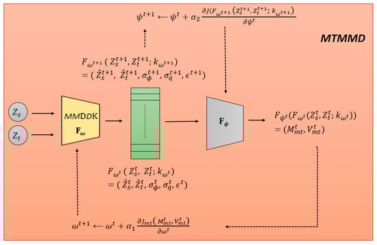
Figure 3. MTMMD network training process.

The primary goal of both updates is to maximize the value of the mean discrepancy function; hence, we aim for both $J_{mt}$ and $J$ to be maximized, with the parameter adjustments being positive multiples of the partial derivatives. The MTMMD network training architecture is illustrated in Figure 3. Since MMDDK and MTMMD are trained together, the gradient values of the MMDDK objective function $J$ are also used to update its parameters $\omega$, modifying Equations (37)–(39). The MTMMD network training and inference algorithms are presented in Algorithms 2 and 3, respectively. Subsequently, the domain adaptation training uses the two-domain mean discrepancy loss function, where the $MM{D}_c^2$ in $L_{dcwmmd}$ is replaced by the meta-learning $M_{mt}^c$ in Equation (40), resulting in the loss function $L_{mtdcwmmd}$ in Equation (41).

$${\omega }^{t+1}\leftarrow {\omega }^t+{\alpha }_1·{\displaystyle \frac{\partial J_{mt}\left(F_{\psi }\left(F_{{\omega }^t}\left(Z_s,Z_t;k_{{\omega }^t}\right)\right)\right)}{\partial {\omega }^t}}$$

(37)

$${\psi }^{t+1}\leftarrow {\psi }^t+{\alpha }_2·{\displaystyle \frac{\partial J\left(F_{{\omega }^{t+1}}\left(Z{\prime }_s,Z{\prime }_t;k_{{\omega }^{t+1}}\right)\right)}{\partial {\psi }^t}}$$

(38)

$${\omega }^{t+1}\leftarrow {\omega }^t+{\alpha }_0·{\displaystyle \frac{\partial J\left(F_{{\omega }^t}\left(Z_s,Z_t;k_{{\omega }^t}\right)\right)}{\partial {\omega }^t}}+{\alpha }_1·{\displaystyle \frac{\partial J_{mt}\left(F_{\psi }\left(F_{{\omega }^t}\left(Z_s,Z_t;k_{{\omega }^t}\right)\right)\right)}{\partial {\omega }^t}}$$

(39)

$$M_{mt}^c=M_{\psi }(F_{\omega }\left(Z_s^c,Z_t^c;k_{\omega }\right)$$

(40)

$$L_{mtdcwmmd}=\beta \prime ·{{\displaystyle \sum }}_{c=1}^C{\left(S_{st}\right)}_{intra}^c+{{\displaystyle \sum }}_{c=0}^C{M}_{mt}^c$$

(41)

The MMDDK model $F_{\omega }$ passes its predictions $F_{{\omega }^t}$ to the meta-module MTMMD $F_{\psi }$, which outputs $F_{{\psi }^t}=\left(M_{mt}^t,V_{mt}^t\right)$, where $M_{mt}^t$ is the mean discrepancy value and $V_{mt}^t$ is the variance. We optimize $\psi$ to ensure that when optimizing the MMDDK model for $J_{mt}$ with $F_{{\omega }^{t+1}}\left(Z{\prime }_s,Z{\prime }_t;k_{{\omega }^{t+1}}\right)$, the updated ${\omega }^{t+1}$ performs better (i.e., there is a higher value of the MMDDK objective function J). To achieve this, we take a gradient step on the meta-module’s objective function $J_{mt}$ to update the MMDDK model parameters ${\omega }^{t+1}$, and then we update $\psi$ by evaluating ${\omega }^{t+1}$ using the MMDDK objective function $J$.

Algorithm 2 Training MTMMD
Input: ${\alpha }_0,{\alpha }_1,{\alpha }_2$; Initialize $\omega$ and $\psi$: sets of parameters for MMDDK Model $F_{\omega }$ and MTMDD Model $F_{\psi }$, $T\leftarrow 10,000$; #$\omega =({\theta }_d,$ ${\sigma }_{\varphi },$ ${\sigma }_q,$ $ϵ)$; for t $\leftarrow$ 0 to T do   $\left(X_s,Y_s\right)=\left\{\left(x_{s1},y_{s1}\right),\left(x_{s2},y_{s2}\right),\dots ,\left(x_{sN},y_{sN}\right)\right\}\leftarrow$mini-batch from ${\Delta }_s$;    $X_t=\left\{x_{t1},x_{t2},\dots ,x_{tN}\right\}\leftarrow$mini-batch from ${\Delta }_t$;    $Z_s\leftarrow F\left(X_s\right);Z_t\leftarrow F\left(X_t\right);$    $\left({\widehat{Z}}_s,{\widehat{Z}}_t,{\sigma }_{\varphi },{\sigma }_q,ϵ\right)\leftarrow F_{\omega }\left(Z_s,Z_t;k_{\omega }\right)$; #${\widehat{Z}}_s=F_d\left(Z_s\right);{\widehat{Z}}_t=F_d\left(Z_t\right);$    #alternatively update parameters ω and ψ:
$M\leftarrow MMDD{K}_u^2\left(Z_s,Z_t;k_{\omega }\right)$;	#using (11)
$V\leftarrow {\sigma }^2\left(Z_s,Z_t;k_{\omega }\right)$;	#using (12) with $\mathsf{\lambda }=0$
$J\leftarrow M/\sqrt{V};$	#using (10)
if t is even then
$\left(M_{mt},V_{mt}\right)\leftarrow F_{\psi }\left({\widehat{Z}}_s,{\widehat{Z}}_t,{\sigma }_{\varphi },{\sigma }_q,ϵ\right)$;      $J_{mt}\leftarrow M_{mt}/\sqrt{V_{mt}}$;
$\omega \leftarrow \omega +{\alpha }_0{\nabla }_{\omega }J+{\alpha }_1{\nabla }_{\omega }{J}_{mt}$;	#maximizing $J_{mt}$
else
$\omega \leftarrow \omega +{\alpha }_2{\nabla }_{\psi }J$;	#maximizing J
end for

Algorithm 3 MTMMD Inferencing

Input: $\omega$ and $\psi$;   $\left(X_s,Y_s\right)=\left\{\left(x_{s1},y_{s1}\right),\left(x_{s2},y_{s2}\right),\dots ,\left(x_{sN},y_{sN}\right)\right\}\leftarrow$mini-batch from ${\Delta }_s$;   $X_t=\left\{x_{t1},x_{t2},\dots ,x_{tN}\right\}\leftarrow$mini-batch from ${\Delta }_t$;   $Z_s\leftarrow F\left(X_s\right);Z_t\leftarrow F\left(X_t\right);$   $\left({\widehat{Z}}_s,{\widehat{Z}}_t,{\sigma }_{\varphi },{\sigma }_q,ϵ\right)\leftarrow F_{\omega }\left(Z_s,Z_t;k_{\omega }\right)$; #${\widehat{Z}}_s=F_d\left(Z_s\right);{\widehat{Z}}_t=F_d\left(Z_t\right)$;   $\left(M_{mt},V_{mt}\right)\leftarrow F_{\psi }\left({\widehat{Z}}_s,{\widehat{Z}}_t,{\sigma }_{\varphi },{\sigma }_q,ϵ\right)$; return $M_{mt}$

3.3. MeTa Discriminative Class-Wise Maximum Mean Discrepancy

The proposed UDA approach, based on MeTa Discriminative Class-Wise Maximum Mean Discrepancy (MCWMMD), includes a feature extractor $\mathit{F}$ for extracting domain-invariant features for the classifier $\mathit{C}$, as shown in Figure 1. Inputs $x_s$ and $x_t$ are fed into the feature extractor $\mathit{F}$, resulting in outputs $z_s=\mathit{F}\left(x_s\right)$ and $z_s=\mathit{F}\left(x_t\right)$. These outputs are then input into the classifier $C$ for classification predictions, producing ${\widehat{\mathcal{l}}}_s=\mathit{C}\left(z_s\right)$ and ${\widehat{\mathcal{l}}}_t=\mathbf{C}\left(z_t\right)$. In practice, the batch size for both the source domain and the target domain is set to $N$, with a total of $C$ category labels. The feature extractor $\mathit{F}$ extracts features from input samples $X_s={\left\{x_{si}\right\}}_{i=1}^N$ and $X_t={\left\{x_{tj}\right\}}_{j=1}^N$, and outputs $Z_s={\left\{z_{si}\right\}}_{i=1}^N$ and $Z_t={\left\{z_{tj}\right\}}_{j=1}^N$, respectively. These features, $Z_s$ and $Z_t$, are then input into the classifier $C$ for classification. In the diagram, $F$ and $C$ are depicted twice to correspond to the data paths of the source and target domains, with a dashed line in between to indicate shared parameters. The MTMMD network will be trained by minimizing the total loss function $L_{total}$, as defined in Equation (42), where $L_{dcwmtmmd}$ is defined in Equation (41) and $L_{cls}^{ls}$ is defined in Equation (44). It is a label-smoothed version of the classification cross-entropy in Equation (43), designed to encourage samples to fall into compact, uniform, and well-separated clusters. The original prediction $y_{si}$ is replaced by $\left(1-\mathsf{\alpha }\right)y_{si}^c+\mathsf{\alpha }/C$, where 1 is a vector of ones with $C$ dimensions, and $\alpha$ is the smoothing parameter. Additionally, $L_{ent}$ represents the predicted label entropy of the target sample, as shown in Equation (45). The network training algorithm for this MCWMMD module is presented in Algorithm 4.

$$L_{total}=L_{mtdcwmmd}+{\omega }_2·L_{cls}^{ls}+{\omega }_3·L_{ent}$$

(42)

$$L_{cls}\left(Z_s,Y_s\right)=-{\displaystyle \frac{1}{n_s}}{{\displaystyle \sum }}_{i=1}^{n_s}{{\displaystyle \sum }}_{c=1}^C{y}_{si}^c\log {\widehat{\mathcal{l}}}_{si}^c$$

(43)

$$L_{cls}^{ls}\left(Z_s,Y_s\right)=-{\displaystyle \frac{1}{n_s}}{{\displaystyle \sum }}_{i=1}^{n_s}{{\displaystyle \sum }}_{c=1}^C\left(\left(1-\alpha \right)y_{si}^c+\alpha /C\right)\log {\widehat{\mathcal{l}}}_{sj}^c$$

(44)

$$L_{ent}\left(Z_t\right)=-{\displaystyle \frac{1}{N}}{{\displaystyle \sum }}_{j=1}^N{{\displaystyle \sum }}_{c=1}^C{\widehat{\mathcal{l}}}_{tj}^c\log {\widehat{\mathcal{l}}}_{tj}^c$$

(45)

Algorithm 4 Training MCWMMD model
Input: ${\Delta }_s,{\Delta }_t,{\beta }_1,{\beta }_2,{\eta }_2;$ Initialize parameters ${\theta }_F$ and ${\theta }_C;$ # train the model parameters ${\theta }_F$ and ${\theta }_C$ on ${\Delta }_s$ and${\Delta }_t;$ repeat until convergence   $\left(X_s,Y_s\right)=\left\{\left(x_{s1},y_{s1}\right),\left(x_{s2},y_{s2}\right),\dots ,\left(x_{sN},y_{sN}\right)\right\}\leftarrow$mini-batch from ${\Delta }_s;$   $X_t=\left\{x_{t1},x_{t2},\dots ,x_{tN}\right\}\leftarrow$ mini-batch from ${\Delta }_t$;   $Z_s\leftarrow$ F$\left(X_s\right);Z_t\leftarrow$ F$\left(X_t\right);$   #generate pseudo labels:
${\widehat{L}}_t=\left\{{\widehat{\mathcal{l}}}_{t1},{\widehat{\mathcal{l}}}_{t2},\dots ,{\widehat{\mathcal{l}}}_{tN}\right\}$ $\leftarrow$ $C\left(F\left(X_t\right)\right)$;	#classify target samples
$Y_t=\left\{y_{t1},y_{t2},\dots ,y_{tN}\right\}\leftarrow \left\{\mathrm{psd}\left({\widehat{\mathcal{l}}}_{t1}\right),\mathrm{psd}\left({\widehat{\mathcal{l}}}_{t2}\right),\dots ,\mathrm{psd}\left({\widehat{\mathcal{l}}}_{tN}\right)\right\};$	#obtain pseudo labels
# $\mathrm{psd}$(($v_1,v_2,\dots ,v_C$)) $=\underset{1\le c\le C}{\mathrm{argmax}}{v}_c$;
# evaluate losses:
$L_{mcwmmd}\left(X_s,X_t\right)=\beta \prime ·{{\displaystyle \sum }}_{c=1}^C{\left(S_{st}\right)}_{intra}^c+{{\displaystyle \sum }}_{c=0}^C{M}_{mt}^c$;	#using (41)
$L_{cls}^{ls}\leftarrow {\displaystyle \frac{1}{N}}{\displaystyle \sum }_{i=1}^N{\displaystyle \sum }_{c=1}^C\left(\left(1-\alpha \right)y_{si}^c+\alpha /C\right)\log {\widehat{\mathcal{l}}}_{sj}^c;$	#using (44)
$L_{ent}\leftarrow$ ${\displaystyle \frac{1}{N}}{\displaystyle \sum }_{j=1}^N{\displaystyle \sum }_{c=1}^C{\widehat{\mathcal{l}}}_{tj}^c\log {\widehat{\mathcal{l}}}_{tj}^c$;	#using (45)
$L_{total}\leftarrow L_{mcwmmd}+{\beta }_1{L}_{cls}^{ls}+{\beta }_2{L}_{ent};$	#using (42)
# update ${\theta }_F$and${\theta }_C$to minimize $L_{total};$
${\theta }_F\leftarrow {\theta }_F-{\eta }_2{\nabla }_{{\theta }_F}{L}_{total};$
${\theta }_C\leftarrow {\theta }_C-{\eta }_2{\nabla }_{{\theta }_C}{L}_{total}$;
end repeat

4. Experimental Results

This section presents a comprehensive evaluation of the JDA approach on standard UDA datasets for image classification tasks. The details of the data preparation process are outlined in Section 4.1, while the experimental setup, including model configurations and parameters, is discussed in Section 4.2. Finally, Section 4.3 provides the experimental results and comparisons with baseline methods to demonstrate the effectiveness of the proposed approach.

4.1. Data Preparation

The proposed approach was evaluated on both digit and office object datasets. The digit datasets used in this study included the MNIST (Modified National Institute of Standards and Technology) database [37], USPS (U.S. Postal Service) [38], and SVHN (Street View House Numbers) [39]. The MNIST and USPS consist of grayscale images of handwritten digits, with the MNIST offering 60,000 training samples and 10,000 testing samples and USPS comprising 9298 images, divided into 7291 training and 2007 testing samples. In contrast, SVHN provides 73,257 color training images and 26,032 testing images, depicting digits captured in a street-view context. Figure 4 shows sample images from the MNIST, USPS, and SVHN, with training samples highlighted in blue.

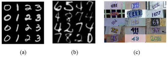
Figure 4. Digit data: (a) MNIST, (b) USPS, and (c) SVHN.

For the office object datasets, we used Office-31 [40] and Office-Home [41]. The Office-31 dataset consists of 4652 images within 31 categories collected from three distinct domains: Amazon (A), which contains images from online merchants; DSLR (D), with high-resolution images taken using a digital SLR camera; and Webcam (W), featuring low-resolution images captured using a web camera. This dataset covers 31 common office object categories, totaling 4110 images. The Office-Home dataset introduces a more complex domain shift, with four distinct domains—Art (Ar), Clipart (Cl), Product (Pr), and Real World (Rw)—spanning 65 object categories and approximately 15,500 images, each offering varied visual styles. Figure 5 and Figure 6 provide sample images from the Office-31 and Office-Home datasets, respectively.

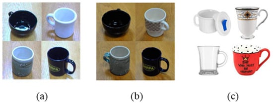
Figure 5. Office-31 data: (a) Webcam, (b) DSLR, and (c) Amazon.

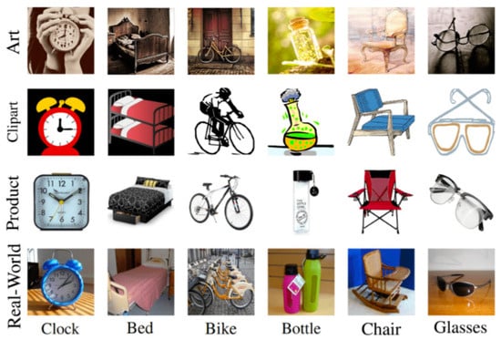
Figure 6. Office-Home data.

4.2. Experimental Setting

An initial learning rate of 0.001 was used for all experiments, decayed by a factor of 0.1 every 10 epochs. The batch size was set to 128 for the digit datasets and 64 for the office object datasets. The Adam optimizer was used with parameters β₁= 0.99 and β₂ = 0.999, and it was chosen for its ability to handle sparse gradients. Training lasted for 50 epochs on the digit datasets and 100 epochs on the office object datasets to ensure convergence. A regularization term of 0.0005 was applied to prevent overfitting. The Gaussian kernel used in the MMD calculations had an initial bandwidth of 1.0, dynamically optimized through the meta-learning framework. At the beginning of each epoch, pseudo-labels for all target domain training data were generated based on the current classifier parameters. This iterative process helped refine domain alignment while maintaining computational efficiency.

Experiments were conducted on a server equipped with NVIDIA RTX 2080 GPUs (manufactured by NVIDIA Corporation, Santa Clara, CA, USA) and 256 GB of system RAM (provided by ADATA, Taiwan). The implementation was carried out using Python with the PyTorch deep learning library (version 1.8), along with NumPy and SciPy for data preprocessing and statistical computations.

4.3. Results

ResNet-18 and ResNet-50 [42] were employed as the network architectures for feature extraction from the digit and office object datasets, respectively. Both models were fine-tuned using pre-trained ImageNet parameters. The performance of the proposed method was evaluated on the above-mentioned datasets: digit datasets, Office-31, and Office-Home. For the digit datasets, we tested domain adaptation between pairs such as MNIST to USPS (M → U), USPS to MNIST (U → M), and SVHN to MNIST (S → M). In the Office-31 dataset, we examined six domain adaptation pairs (e.g., Amazon to DSLR (A → D) and Webcam to DSLR (W → D)). For the Office-Home dataset, we created 12 domain adaptation pairs across four domains (Art, Clipart, Product, and Real-World), including examples like Art to Clipart (Ar → Cl), Product to Real-World (Pr → Rw), and so on.

Table 2 compares our method with several domain adaptation techniques on the digit datasets, including ADDA [5], ADR [43], CDAN [44], CyCADA [12], SWD [45], SHOT [46], and our previous work, DCWMMD [28]. Table 3 provides a comparison of the Office-31 dataset, including methods such as that by Wang et al. [25], DAN [6], DANN [4], ADDA, MADA [47], SHOT, CAN [3], MDGE [2], DACDM [9], CDCL [10], DMP [11], and DCWMMD [28]. Table 4 compares the results of the Office-Home dataset with methods like that used by Wang et al., DAN, DACDM [9], DMP [11], and DCWMMD. Please note that the results are directly referenced from published papers. The best-performing method for each source-to-target combination is highlighted in bold. The bold numbers in the tables indicate the best-performing accuracy for each source-to-target combination. The “Source-only” category represents a classifier trained solely on source data, while “Target-supervised” denotes a classifier trained and tested on target domain data, typically representing lower and upper bounds for domain adaptation performance.

Table 2. Accuracies (%) of several approaches on some digit datasets.

$\mathbf{Source}\to$Target Methods	$\mathbf{M}\to$U	$\mathbf{U}\to$M	$\mathbf{S}\to$M	Average
Source-only	69.6	82.2	67.1	73.0
ADDA [5]	90.1	89.4	76.0	85.2
ADR [43]	93.1	93.2	95.0	93.8
CDAN [44]	98.0	95.6	89.2	94.3
CyCADA [12]	96.5	95.6	90.4	94.2
SWD [45]	97.1	98.1	98.9	98.0
SHOT [46]	97.8	97.6	99.0	98.1
DCWMMD [28]	98.0	98.2	98.8	98.3
MCWMMD	98.5	98.3	98.9	98.6
Target-supervised	98.9	99.4	99.4	99.2

Table 3. Accuracies (%) for domain adaptation experiments on the Office-31 dataset.

Methods	$\mathbf{A}\to$D	$\mathbf{A}\to$W	$\mathbf{D}\to$A	$\mathbf{D}\to$W	$\mathbf{W}\to$A	$\mathbf{W}\to$D	Average
Source-only	68.90	68.40	62.50	96.70	60.70	99.30	76.10
Wang et al. [25]	90.80	88.90	75.48	98.50	75.20	99.80	88.10
DAN [6]	78.60	80.50	63.60	97.10	62.80	99.60	80.40
DANN [4]	79.70	82.00	68.20	96.90	67.40	99.10	82.20
ADDA [5]	77.80	86.20	69.50	96.20	68.90	98.40	82.90
MADA [47]	87.80	90.00	70.30	97.40	66.40	99.60	85.20
SHOT [46]	93.90	90.10	75.30	98.70	75.00	99.90	88.80
CAN [3]	95.00	94.50	78.00	99.10	77.00	99.80	90.60
MDGE [2]	90.60	89.40	69.50	98.90	68.40	99.80	86.10
DACDM [9]	95.31	95.51	78.26	98.58	78.43	99.93	91.01
CDCL [10]	96.00	96.00	77.20	99.20	75.50	100	90.60
DMP [11]	91.00	93.00	71.40	99.00	70.20	100	87.40
DCWMMD [28]	96.30	94.90	77.90	99.50	76.50	99.60	90.80
MCWMMD	96.70	96.60	78.40	99.60	78.60	99.83	91.62
Target-supervised	98.00	98.70	86.00	98.70	86.00	98.00	94.30

Table 4. Accuracies (%) for domain adaptation experiments on the Office-Home dataset.

Methods	$\mathbf{Ar}\to$Cl	$\mathbf{Ar}\to$Pr	$\mathbf{Ar}\to$Rw	$\mathbf{Cl}\to$Ar	$\mathbf{Cl}\to$Pr	$\mathbf{Cl}\to$Rw	$\mathbf{Pr}\to$Ar	$\mathbf{Pr}\to$Cl	$\mathbf{Pr}\to$Rw	$\mathbf{Rw}\to$Ar	$\mathbf{Rw}\to$Cl	$\mathbf{Rw}\to$Pr	Average
source-only	28.07	38.30	42.05	26.15	40.57	39.14	25.94	28.40	46.61	27.10	30.12	55.35	35.65
Wang et al. [25]	58.44	77.79	79.32	61.60	72.81	73.03	62.71	55.33	78.91	70.42	60.09	83.24	69.47
DAN [6]	43.60	57.00	67.90	45.80	56.50	60.40	44.00	43.60	67.70	63.10	51.50	74.30	56.28
DANN [4]	45.60	59.30	70.10	47.00	58.50	60.90	46.10	43.70	68.50	63.20	51.80	76.80	57.63
DACDM [9]	60.94	79.27	83.34	69.67	81.53	80.40	65.06	58.97	83.45	75.90	65.61	85.99	74.18
DMP [11]	59.00	81.20	86.30	68.10	72.80	78.80	71.20	57.60	84.90	77.30	61.50	82.90	73.50
DCWMMD [28]	59.69	80.23	81.31	70.24	79.45	82.65	69.20	57.87	85.12	74.80	64.20	83.14	73.99
MCWMMD	62.21	81.46	83.92	71.45	79.98	83.42	71.08	59.12	85.64	76.10	65.32	85.48	75.43
target-supervised	93.24	92.35	92.08	91.16	92.35	92.08	91.16	93.24	92.08	91.16	93.24	92.35	92.21

In Table 2, our method achieves an average accuracy of 98.60% across digit datasets, outperforming other methods and closely approaching the target-supervised scenario. This highlights the robustness of our approach in aligning domain distributions and achieving class-wise alignment. Table 3 presents the results of the Office-31 dataset, where our method achieved an average accuracy of 91.62%, consistently outperforming other unsupervised adaptation methods and closely matching the target-supervised benchmark. This result underscores the effectiveness of our Class-Wise MMD optimization method in adapting complex, real-world data. In Table 4, our method achieves an average accuracy of 75.43% on the Office-Home dataset, a challenging multi-domain setting with diverse visual characteristics. These results highlight the adaptability and robustness of our approach as it generalizes effectively across multiple domains and significantly closes the gap with the target-supervised benchmark. This performance demonstrates our method’s capability to handle complex domain shifts while maintaining high accuracy across diverse visual domains.

t-SNE (t-distributed Stochastic Neighbor Embedding) [48] is a nonlinear dimensionality reduction technique commonly used to visualize high-dimensional data in a lower-dimensional space (typically 2D or 3D). By preserving local structures within the data, t-SNE excels in representing clusters and relationships, making it particularly useful for visualizing stochastic settings and complex data distributions. In this study, we employ t-SNE to visualize the feature representations learned by our model for both the source and target domains, highlighting the effectiveness of the proposed domain adaptation approach.

Columns (a) and (b) of Figure 7 depict the distributions of source features and target features, respectively, with different digits represented by distinct colors. Specifically, the 10 colors correspond to the digits 0 through 9, where each color uniquely represents a digit for clear differentiation in the visualization. Column (c) of Figure 7 provides an integrated view of both distributions to highlight their alignment. As observed, the source and target features are well aligned, demonstrating the effectiveness of our approach. The t-SNE visualization effectively highlights the alignment between source and target feature distributions, reflecting the improved feature alignment achieved by our method compared to the baseline.

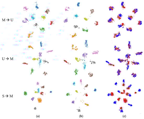
Figure 7. t-SNE visualization of three tasks on digit datasets: (a) source, (b) target, and (c) source (red color) + target (blue color) (best viewed in color).

5. Discussion and Conclusions

The proposed method, MeTa Discriminative Class-Wise MMD (MCWMMD), represents a significant advancement in unsupervised domain adaptation by integrating meta-learning with a Class-Wise Maximum Mean Discrepancy (MMD) approach. While traditional MMD methods align overall distributions between source and target domains, they often fail to achieve precise class-wise alignment, reducing feature distinguishability and generalization performance. MCWMMD addresses these limitations by introducing dynamic kernel adaptability and a focus on class-wise alignment, resulting in robust and domain-invariant representations.

A key innovation of MCWMMD is its dynamic kernel adaptability, achieved through a meta-module that adjusts kernel parameters based on class-specific features. This enables more precise domain alignment compared to traditional static kernels, significantly enhancing alignment and generalization. The alternating training process between the feature extractor and the meta-module, inspired by adversarial training, further refines the model’s ability to handle complex domain shifts. However, this adaptability introduces computational complexity, which could be a limitation for time-sensitive applications. Future research could explore simplifying the meta-module to reduce overhead while preserving adaptability.

The method’s class-wise alignment approach applies MMD in a class-specific manner, ensuring that each class is individually aligned between source and target domains. This produces compact, domain-invariant, and class-discriminative feature clusters, ultimately improving cross-domain classification performance. However, its reliance on accurate pseudo-labels for class-wise alignment may lead to errors when the pseudo-label quality is low. Developing robust pseudo-labeling strategies is a crucial direction for future research.

MCWMMD is also optimized for scalability through efficient batch processing and streamlined meta-module training, enabling practical application to large datasets without compromising alignment accuracy. However, scaling it extremely large or dynamically evolving datasets remains a challenge. Future work could investigate distributed or online learning paradigms to extend the method’s applicability to these scenarios.

Despite its strengths, MCWMMD involves complex meta-module training and adversarial-like processes, which may pose implementation challenges, particularly for practitioners with limited computational resources. Further validation in real-world scenarios with highly diverse and complex domain shifts is also needed. Promising future directions include simplifying the meta-module for enhanced accessibility, improving pseudo-labeling mechanisms, and extending the method to handle online and incremental domain adaptation for dynamic datasets. Additionally, exploring cross-domain generalization to unseen categories or settings could further enhance the method’s adaptability.

In summary, MCWMMD advances unsupervised domain adaptation by combining meta-learning with a Class-Wise MMD approach, addressing the limitations of traditional techniques. Its dynamic kernel adaptability and focus on class-wise alignment enable robust feature alignment and generalization. While challenges such as computational complexity and reliance on pseudo-labels remain, MCWMMD provides a strong foundation for future innovations, paving the way for more adaptable and generalizable deep learning models.

References

- Lin, Y.; Chen, J.; Cao, Y.; Zhou, Y.; Zhang, L.; Tang, Y.Y.; Wang, S. Cross-domain recognition by identifying joint subspaces of source domain and target Domain. IEEE Trans. Cybern. 2017, 47, 1090–1101. [Google Scholar] [CrossRef]
- Khan, S.; Guo, Y.; Ye, Y.; Li, C.; Wu, Q. Mini-batch dynamic geometric embedding for unsupervised domain adaptation. Neural Process. Lett. 2023, 55, 2063–2080. [Google Scholar] [CrossRef]
- Zhang, W.; Ouyang, W.; Li, W.; Xu, D. Collaborative and adversarial network for unsupervised domain adaptation. In Proceedings of the 2018 IEEE/CVF Conference on Computer Vision and Pattern Recognition, Salt Lake City, UT, USA, 18–23 June 2018. [Google Scholar] [CrossRef]
- Ganin, Y.; Ustinova, E.; Ajakan, H.; Germain, P.; Larochelle, H.; Laviolette, F.; Marchand, M.; Lempitsky, V. Domain adversarial training of neural networks. J. Mach. Learn. Res. 2016, 17, 1–35. [Google Scholar] [CrossRef]
- Tzeng, E.; Hoffman, J.; Saenko, K.; Darrell, T. Adversarial discriminative domain adaptation. In Proceedings of the 2017 IEEE Conference on Computer Vision and Pattern Recognition (CVPR), Honolulu, HI, USA, 21–26 July 2017; pp. 2962–2971. [Google Scholar] [CrossRef]
- Long, M.; Cao, Y.; Wang, J.; Jordan, M.I. Learning transferable features with deep adaptation networks. In Proceedings of the 32nd International Conference on International Conference on Machine Learning, Lille, France, 6–11 July 2015; Volume 37, pp. 97–105. [Google Scholar]
- Vettoruzzo, A.; Bouguelia, M.-R.; Rögnvaldsson, T.S. Meta-learning for efficient unsupervised domain adaptation. Neurocomputing 2024, 574, 127264. [Google Scholar] [CrossRef]
- Liu, X.; Yoo, C.; Xing, F.; Oh, H.; El Fakhri, G.; Kang, J.-W.; Woo, J. Deep Unsupervised Domain Adaptation: A Review of Recent Advances and Perspectives. arXiv 2022, arXiv:2208.07422v1. [Google Scholar] [CrossRef]
- Zhang, Y.; Chen, S.; Jiang, W.; Zhang, Y.; Lu, J.; Kwok, J.T. Domain-Guided Conditional Diffusion Model for Unsupervised Domain Adaptation. arXiv 2023, arXiv:2309.14360v1. [Google Scholar] [CrossRef] [PubMed]
- Wang, R.; Wu, Z.; Weng, Z.; Chen, J.; Qi, G.-J.; Jiang, Y.-G. Cross-Domain Contrastive Learning for Unsupervised Domain Adaptation. arXiv 2022, arXiv:2106.05528v2. [Google Scholar] [CrossRef]
- Luo, Y.-W.; Ren, C.-X.; Dai, D.-Q.; Yan, H. Unsupervised Domain Adaptation via Discriminative Manifold Propagation. IEEE Trans. Pattern Anal. Machine Intell. 2022, 44, 1653–1669. [Google Scholar] [CrossRef] [PubMed]
- Hoffman, J.; Tzeng, E.; Park, T.; Zhu, J.Y.; Isola, P.; Saenko, K. Cycada: Cycle-consistent adversarial domain adaptation. In Proceedings of the 35th International Conference on Machine Learning, Stockholm, Sweden, 10–15 July 2018; pp. 1989–1998. [Google Scholar]
- Saito, K.; Watanabe, K.; Ushiku, Y.; Harada, T. Maximum Classifier Discrepancy for Unsupervised Domain Adaptation. arXiv 2018, arXiv:1712.02560v4. [Google Scholar] [CrossRef]
- Chen, Y.; Li, W.; Sakaridis, C.; Dai, D.; Van Gool, L. Domain adaptive faster R-CNN for object detection in the wild. In Proceedings of the IEEE Conference on Computer Vision and Pattern Recognition, Salt Lake City, UT, USA, 18–23 June 2018; pp. 3339–3348. [Google Scholar]
- Si, S.; Tao, D.; Geng, B. Bregman divergence based regularization for transfer subspace learning. IEEE Trans. Knowl. Data Eng. 2010, 22, 929–942. [Google Scholar] [CrossRef]
- Blitzer, J.; Crammer, K.; Kulesza, A.; Pereira, F.; Wortman, J. Learning bounds for domain adaptation. In Proceedings of the Annual Conference on Neural Information Processing Systems, Vancouver, BC, Canada, 3–6 December 2007; pp. 129–136. [Google Scholar]
- Ding, Z.; Fu, Y. Robust transfer metric learning for image classification. IEEE Trans. Image Process. 2017, 26, 660–670. [Google Scholar] [CrossRef]
- Gretton, A.; Borgwardt, K.; Rasch, M.; Sch, B.; Smola, A. A kernel two-sample test. J. Mach. Learn. Res. 2012, 13, 723–773. [Google Scholar]
- Pan, S.J.; Tsang, I.W.; Kwok, J.T.; Yang, Q. Domain adaptation via transfer component analysis. IEEE Trans. Neural Netw. 2011, 22, 199–210. [Google Scholar] [CrossRef] [PubMed]
- Song, L.; Gretton, A.; Bickson, D.; Low, Y.; Guestrin, C. Kernel belief propagation. In Proceedings of the 14th International Conference on Artificial Intelligence and Statistics, Fort Lauderdale, FL, USA, 11–13 April 2011; pp. 707–715. [Google Scholar]
- Park, M.; Jitkrittum, W.; Sejdinovic, D. K2-ABC: Approximate bayesian computation with kernel embeddings. In Proceedings of the 19th International Conference on Artificial Intelligence and Statistics, Cadiz, Spain, 9–11 May 2016; pp. 398–407. [Google Scholar]
- Li, Y.; Swersky, K.; Zemel, R.S. Generative moment matching networks. In Proceedings of the 32nd International Conference on Machine Learning, Lille, France, 6–11 July 2015; pp. 1718–1727. [Google Scholar]
- Liu, F.; Xu, W.; Lu, J.; Zhang, G.; Gretton, A.; Sutherland, D. Learning deep kernels for non-parametric two-sample tests. arXiv 2020, arXiv:2002.09116. [Google Scholar]
- Long, M.; Wang, J.; Ding, G.; Sun, J.; Yu, P.S. Transfer feature learning with joint distribution adaptation. In Proceedings of the IEEE International Conference on Computer Vision, Sydney, Australia, 1–8 December 2013; IEEE Computer Society: Sydney, Australia, 2013; pp. 2200–2207. [Google Scholar]
- Wang, W.; Li, H.; Ding, Z.; Wang, Z. Rethink maximum mean discrepancy for domain adaptation. arXiv 2020, arXiv:2007.00689. [Google Scholar] [CrossRef]
- Devroye, L.; Lugosi, G. Combinatorial Methods in Density Estimation; Springer: New York, NY, USA, 2001. [Google Scholar] [CrossRef]
- Baraud, Y.; Birgé, L. Rho-estimators revisited: General theory and applications. Ann. Statist. 2018, 46, 3767–3804. [Google Scholar] [CrossRef]
- Lin, H.-W.; Tsai, Y.; Lin, H.J.; Yu, C.-H.; Liu, M.-H. Unsupervised domain adaptation deep network based on discriminative class-wise MMD. AIMS Math. 2024, 9, 6628–6647. [Google Scholar] [CrossRef]
- Andrychowicz, M.; Denil, M.; Colmenarejo, S.G.; Hoffman, M.W.; Pfau, D.; Schaul, T.; de Freitas, N. Learning to learn by gradient descent by gradient descent. arXiv 2016, arXiv:1606.04474v2. [Google Scholar] [CrossRef]
- Finn, C.; Abbeel, P.; Levine, S. Model-agnostic meta-learning for fast adaptation of deep networks. In Proceedings of the 34th International Conference on Machine Learning, Sydney, Australia, 6–11 August 2017. [Google Scholar]
- Aronszajn, N. Theory of reproducing kernels. Trans. Am. Math. Soc. 1950, 68, 337–404. [Google Scholar] [CrossRef]
- Zheng, S.; Ding, C.; Nie, F.; Huang, H. Harmonic mean linear discriminant analysis. IEEE Trans. Knowl. Data Eng. 2019, 31, 1520–1531. [Google Scholar] [CrossRef]
- Borgwardt, K.M.; Gretton, A.; Rasch, M.J.; Kriegel, H.-P.; Sch, B.; Smola, A.J. Integrating structured biological data by kernel maximum mean discrepancy. Bioinformatics 2006, 22, e49–e57. [Google Scholar] [CrossRef]
- Gao, W.; Shao, M.; Shu, J.; Zhuang, X. Meta-BN Net for few-shot learning. Front. Comput. Sci. 2023, 17, 171302. [Google Scholar] [CrossRef]
- Bechtle, S.; Molchanov, A.; Chebotar, Y.; Grefenstette, E.; Righetti, L.; Sukhatme, G.; Meier, F. Meta-learning via learned loss. arXiv 2019, arXiv:1906.05374. [Google Scholar]
- Müller, R.; Kornblith, S.; Hinton, G. When does label smoothing help? In Proceedings of the Conference on Computer Vision and Pattern Recognition (CVPR), Seattle, WA, USA, 13–19 June 2020. [Google Scholar]
- LeCun, Y.; Bottou, L.; Bengio, Y.; Haffner, P. Gradient-based learning applied to document recognition. Proc. IEEE 1998, 86, 2278–2324. [Google Scholar] [CrossRef]
- Hull, J.J. A database for handwritten text recognition research. IEEE Trans. Pattern Anal. Machine Intell. 1994, 16, 550–555. [Google Scholar] [CrossRef]
- SVHN Dataset. Available online: https://www.openml.org/search?type=data&sort=runs&id=41081&status=active (accessed on 1 March 2024).
- Saenko, K.; Kulis, B.; Fritz, M.; Darrell, T. Adapting visual category models to new domains. In Lecture Notes in Computer Science; Springer: Berlin/Heidelberg, Germany, 2010; Volume 6314, pp. 213–226. [Google Scholar] [CrossRef]
- Office-Home Dataset. Available online: https://www.hemanthdv.org/officeHomeDataset.html (accessed on 1 March 2024).
- He, K.; Zhang, X.; Ren, S.; Sun, J. Deep residual learning for image recognition. In Proceedings of the Conference on Computer Vision and Pattern Recognition (CVPR), Las Vegas, NV, USA, 27–30 June 2016; pp. 770–778. [Google Scholar] [CrossRef]
- Saito, K.; Ushiku, Y.; Harada, T.; Saenko, K. Adversarial dropout regularization. arXiv 2018, arXiv:1711.01575. [Google Scholar] [CrossRef]
- Long, M.; Cao, Z.; Wang, J.; Jordan, M.I. Conditional adversarial domain adaptation. In Proceedings of the 32nd Conference on Neural Information Processing Systems, Montreal, QC, Canada, 3–8 December 2018; pp. 1647–1657. [Google Scholar]
- Lee, C.Y.; Batra, T.; Baig, M.H.; Ulbricht, D. Sliced wasserstein discrepancy for unsupervised domain adaptation. In Proceedings of the IEEE/CVF Conference on Computer Vision and Pattern Recognition (CVPR), Long Beach, CA, USA, 15–20 June 2019; pp. 10285–10295. [Google Scholar]
- Liang, J.; Hu, D.; Feng, J. Do we really need to access the source data? Source hypothesis transfer for unsupervised domain adaptation. In Proceedings of the 37th International Conference on Machine Learning, Virtual, 13–18 July 2020; Volume 119, pp. 6028–6039. [Google Scholar]
- Pei, Z.; Cao, Z.; Long, M.; Wang, J. Multi-adversarial domain adaptation. In Proceedings of the 32nd AAAI Conference on Artificial Intelligence, New Orleans, LA, USA, 2–7 February 2018; Volume 32. [Google Scholar] [CrossRef]
- van der Maaten, L.; Hinton, G. Visualizing data using t-SNE. J. Mach. Learn. Res. 2008, 9, 2579–2605. Available online: http://www.jmlr.org/papers/v9/vandermaaten08a.html (accessed on 1 March 2024).
Disclaimer/Publisher’s Note: The statements, opinions and data contained in all publications are solely those of the individual author(s) and contributor(s) and not of MDPI and/or the editor(s). MDPI and/or the editor(s) disclaim responsibility for any injury to people or property resulting from any ideas, methods, instructions or products referred to in the content. |
© 2025 by the authors. Licensee MDPI, Basel, Switzerland. This article is an open access article distributed under the terms and conditions of the Creative Commons Attribution (CC BY) license (https://creativecommons.org/licenses/by/4.0/).