Abstract
Four explicit numerical schemes are collected, which are stable and efficient for the diffusion equation. Using these diffusion solvers, several new methods are constructed for the nonlinear Huxley’s equation. Then, based on many successive numerical case studies in one and two space dimensions, the least performing methods are gradually dropped out to keep only the best ones. During the tests, not only one but all the relevant time step sizes are considered, and for them, running-time measurements are performed. A major aspect is computational efficiency, which means that an acceptable solution is produced in the shortest possible time. Parameter sweeps are executed for the coefficient of the nonlinear term, the stiffness ratio, and the length of the examined time interval as well. We obtained that usually, the leapfrog–hopscotch method with Strang-type operator-splitting is the most efficient and reliable, but the method based on the Dufort–Frankel scheme can also be very efficient.
Keywords:
nonlinear PDEs; diffusion–reaction equations; Huxley’s equation; explicit numerical methods; stiff equations MSC:
35K20; 35K57; 65M06l
1. Introduction
Nonlinear reaction–diffusion partial differential equations (PDEs) have an important role in modeling different phenomena in many branches of science. We examine Huxley’s equation [1] in this paper assuming the following format:
Several clever methods are proposed to solve these and similar PDEs, such as the shifted Chebyshev spectral collocation method [5], semi-analytical methods [6,7], the homotopy perturbation method [8], different versions of physics-informed neural networks (PINNs) [9,10], the weighted average method [11], and exact as well as nonstandard finite difference schemes (NSFD) [12]. Most of these approaches are constructed and tested for specific circumstances where the media are homogeneous, and/or the number of space dimensions is small, and the spatial mesh is uniform and consists of not very many nodes. There are some counterexamples, e.g., when a partially implicit scheme [13], coarse-grain models [14], or the asymptotic theory [15] were used in heterogeneous media, but these can be considered as exceptions. Nevertheless, under the mentioned specific circumstances, the weak points of the proposed algorithms do not always manifest. Moreover, some of these algorithms were developed aiming, most importantly, high accuracy. However, in most applications, there are non-negligible inaccuracies in the input data, and the models themselves contain simplifications that can cause even a few percent deviation from the measurements. Due to these limitations, the main goal should not be to press down the relative errors below, e.g., 10−8, but to develop methods which are, on the one hand, fast in higher dimensions as well, and, on the other hand, robust, i.e., reliable for all possible parameter combinations.
Most explicit numerical algorithms have a severely constrained stability region [16]. If the time step size is greater than a certain threshold, often called the Courant–Friedrichs–Lewy (CFL) limit, the solution is predicted to explode even for the linear diffusion or heat equation. The heterogeneity in the physical media implies a space-dependent α coefficient [17], which results in a high stiffness ratio and a relatively small CFL limit for the explicit approaches. This is especially well-known when one uses the method of lines, where the PDE is first spatially discretized, and an ODE solver, such as a Runge–Kutta (RK) scheme, solves the resulting system of ODEs. This is true for low-order explicit schemes, such as the FTCS (forward-time central space) or semi-explicit [18] methods, as well as higher order techniques, including the standard fourth-order RK method and Strong-Stability-Preserving Runge–Kutta Methods [19,20].
Although step size restrictions may occasionally be necessary, implicit approaches, such as the technique called shifted airfoil collocation, proposed by Anjuman et al. [21] for nonlinear drift-diffusion–reaction equations, offer superior stability qualities [22]. The most restricting problem is that implicit methods need the solution of a system of nonlinear algebraic equations, which can take a lot of time and memory if the system is big, which is typical in two or three space dimensions. Despite this, implicit techniques are frequently used to solve these and similar equations [23], for example, backward implicit and Crank–Nicolson (CrN) schemes with and without linearization [24]. Rufai et al. proposed a novel hybrid block method for the FitzHugh–Nagumo equation with time-dependent coefficients [25]. Their method is also implicit, and the Newton method is used to handle the nonlinearity. Furthermore, in the case of high stiffness, the diffusion term is occasionally even considered exactly [26]. Manaa and Sabawi [27] solved Equation (3) using the CrN and explicit (Euler) methods. They found that although the explicit technique requires shorter execution times, the CrN method is more accurate and does not have significant stability problems, as was to be predicted. A finite-difference numerical scheme with good qualitative properties was proposed by Macías-Díaz for the Burgers–Huxley equation [28]. However, his algorithm only has favorable features for short time step sizes below the CFL number since he employed the explicit Euler time discretization for the diffusion factor. This also applies to most NSFD algorithms, which were applied, for example, for the Fisher and Nagumo equations [3,29,30] and for cross-diffusion equations [31,32]. Our research group constructs and tests explicit numerical methods possessing excellent stability properties. A couple of these methods have been known for a long time, but they have been used for nonlinear PDEs containing a diffusion term only a few times, much less than they deserve. For example, the Dufort–Frankel scheme was successfully applied for the two-dimensional Sine–Gordon equation [33]. The nonlinear term is treated by a predictor–corrector-type operator-splitting. Gasparin et al. also applied the Dufort–Frankel scheme to nonlinear moisture transfer in porous materials [34]. The odd–even hopscotch method was utilized to solve the Frank–Kamenetskii equation by Harley [35]. These algorithms always showed a good performance; nevertheless, their investigations were usually not continued. Furthermore, in most scientific works, where the performance of numerical methods is tested, the parameters, such as the constants α, β and the space and time step size are fixed, and only a small number of numerical methods are compared. Our goal in this work is to extensively investigate the performance of some methods for Huxley’s equation under a large number of parameter combinations, for example, for less-stiff and very stiff systems. Hence, in Section 2, the spatial discretization of Equation (1) is performed not only for the most basic one-dimensional system with constant α but also for the most general case. In Section 3, we review four numerical methods that were proven to be very efficient when applied to the diffusion equation. All of these diffusion solvers are explicit and unconditionally stable in the linear case. In Section 4, we construct numerous ways to handle the nonlinear reaction term, as well as briefly present methods that will be used for comparison purposes. With these, we gain more than 40 different numerical methods to test for Huxley’s equation. In Section 5, we perform the first round of the numerical experiments, which constitutes five concrete case studies. Based on the comparison of the errors for several time step sizes, we exclude most of the methods from further investigation and keep only 13. In the second round of numerical experiments in Section 6, three case studies are performed in large two-dimensional systems with running time measurement to choose the top seven most efficient methods. Only these seven methods are used in Section 7 to examine how their performance depends on some parameters, such as the strength of the nonlinear reaction term and the CFL limit of the system. Section 8 provides a summary of the findings and suggests methods that should be used under specific circumstances.
We do not know any other work in which so many methods are tested for such a large number of parameter combinations for any nonlinear PDE. The best few among these tested methods are very efficient and reliable, and they have never been applied to Huxley’s equation before. These are the main novelties in our work.
2. The Studied Equation and the Spatial Discretization
We start by discretizing the pure diffusion or heat equation because the reaction term is entirely local. The first step is the simplest and most standard discretization by equidistant nodes of the space interval . The second spatial derivatives are subjected to the well-known central difference approximation, leading to the well-known ODE system
for the nodes with index . The M matrix, which is tridiagonal in the one-dimensional example, contains only a few of nonzero elements as follows:
The boundary conditions (BCs) specify the first and last row. For example, the first and last nodes’ time development will be provided directly in the case of Dirichlet BCs; thus, . The matrix form of the ODE system (4) can be reformulated as follows:
where . Our goal includes performing experiments in general cases where the geometrical and material characteristics of the simulated system are different in different spatial regions. It is necessary to adapt space discretization and subsequent techniques to reflect this generality level. If the media property α is dependent on the space variable while we remain in 1D, the PDE
can be used. We can discretize the parameter α and, simultaneously, to obtain
The average diffusivity between cell i and its (left) neighbor may be denoted by αi,i−1. In practice, it can be approximated by its value between these two nodes. With this, we have
This is a generalized version of Equation (4). We can build a highly adaptable resistance–capacitance model by taking cells into account rather than nodes. The volume of these cells can be expressed as in the case of a one-dimensional equidistant mesh. A cell’s capacity is equal to its volume in the case of the most basic diffusion: . Between two cells, the resistance may be calculated simply as . A generalized ODE system for the time derivative of each cell variable u in one space dimension can be obtained using these:
It is easy to see that this RC model with Equation (7) is indeed a generalization of the original model based on equidistant nodes, in which Equation (4) expressed the time development of the node variables. Hence, if a numerical method works for the general RC model, it will work for the special case as well. Furthermore, Equation (7) can be expressed in the same matrix form as Equation (6), but with entries that depend on the resistances and capacities.
We will also work in two space dimensions, where the numbering of the cells begins along the x-directional (horizontal) rows starting from 1 to and then along the x-axis again from to , and so on. Now, an ODE system (7) can be straightforwardly generalized to two space dimensions as follows:
The last equation is valid since the resistances are infinity for non-adjacent cells. Additional information about the discretization using this resistance–capacitance model can be found, for example, in [36].
In 2D numerical experiments, we usually take zero-Neumann BCs into account. The RC model will implement these in a straightforward manner: the matrix components that are responsible for conduction across the borders vanish when those resistances are regarded as infinite. In this instance, the conserved quantity is represented by the system matrix M’s zero eigenvalue. All other eigenvalues M are negative due to the Second Law of Thermodynamics. The eigenvalues with the (nonzero) least and highest absolute values, respectively, are indicated by λMIN and λMAX. The standard definition of the problem’s stiffness ratio is SR = λMAX/λMIN. In addition to it, the CFL limit provides an accurate estimate of the maximum time step size that can be used for the semi-discretized linear diffusion problem (4), (7), or (8) using the explicit Euler (first-order explicit RK) scheme. Similar threshold time step sizes can be obtained for higher-order explicit RK schemes, such as for the fourth-order RK schemes: . This CFL threshold and the stiffness ratio will be utilized in this paper to describe how difficult it is to solve the problem. We must emphasize again that the unconditionally stable schemes employed in this work have no time step size restrictions for the linear diffusion problem due to stability considerations.
The simplest uniform discretization
will always be used for the time variable.
3. The Examined Diffusion Solver Methods
We provide essential details regarding the algorithms that solve an equation without the nonlinear term. Since we mostly employ the more general forms in this study, only they are required.
For the 1D equidistant mesh, such as in Equation (1), the standard mesh ratio of is used in many publications and textbooks. In the case of the general mesh, the following notations are going to be used:
While the second quantity reflects the status and influence of the neighbors of cell i, the first quantity is the generalization of the mesh ratio.
- 1.
- The first method is called the CCL algorithm, which is the abbreviation for Constant–Constant–Linear neighbor. It is a one-step but three-stage method recently published by our group [37], where the constant-neighbor (CNe) formula is applied in the first and second stages. The first stage is a predictor with a h/3-sized time step:
Then, the first corrector stage comes
Finally, a full time step is taken with the linear-neighbor (LNe) formula in the third stage:
During the calculations, the quantities must be refreshed after each stage:
and , respectively. The CCL method has third-order temporal accuracy, and, similarly to the following three methods, it is proven to be unconditionally stable for the heat equation.
- 2.
- The Dufort–Frankel (DF) method is a classic example of the explicit and stable methods [38] (p. 313), which is second-order in time. We adapted it to the general case, where the following formula must be used:
As can be seen, it is a two-step, one-stage method (the formula includes ). Since it is not self-starting, the calculation must be performed by another method. We use the so-called UPFD (unconditional finite difference) formula for this purpose:
- 3.
- The original odd–even hopscotch (OOEH) method was discovered more than 50 years ago [39]. It requires a special spatial and temporal structure. In essence, the mesh must be bipartite, i.e., it is divided into two parts, the so-called odd and even nodes (or cells), where the closest neighbor of the even cells is odd, and vice versa. First, the FTCS formula is applied to the odd cells, followed by the BTCS (Backward-time Central-space) formula, which is based on implicit Euler time discretization. After every time step, the odd and even labels are switched, as it is illustrated in Figure 1. The equations used are as follows:
.
where the new concentration data are used to calculate in the same manner as Ai in Equation (12), essentially making the implicit formula explicit.
- 4.
- The recently invented leapfrog–hopscotch (LH) approach [40] also requires the odd–even space structure. Moreover, it has a structure made up of many full time steps and two half time steps. Using the initial values, the calculation begins by taking a half-sized time step for the odd nodes. Full time steps are then taken strictly alternately for the even and odd nodes until the last time step is reached, which should be halved for odd nodes to reach the same final time point as the even nodes, as shown in Figure 1.

Figure 1.
The structures of original odd–even hopscotch (OOEH), leapfrog–hopscotch (LH), and Dufort–Frankel (DF) methods.
Figure 1.
The structures of original odd–even hopscotch (OOEH), leapfrog–hopscotch (LH), and Dufort–Frankel (DF) methods.
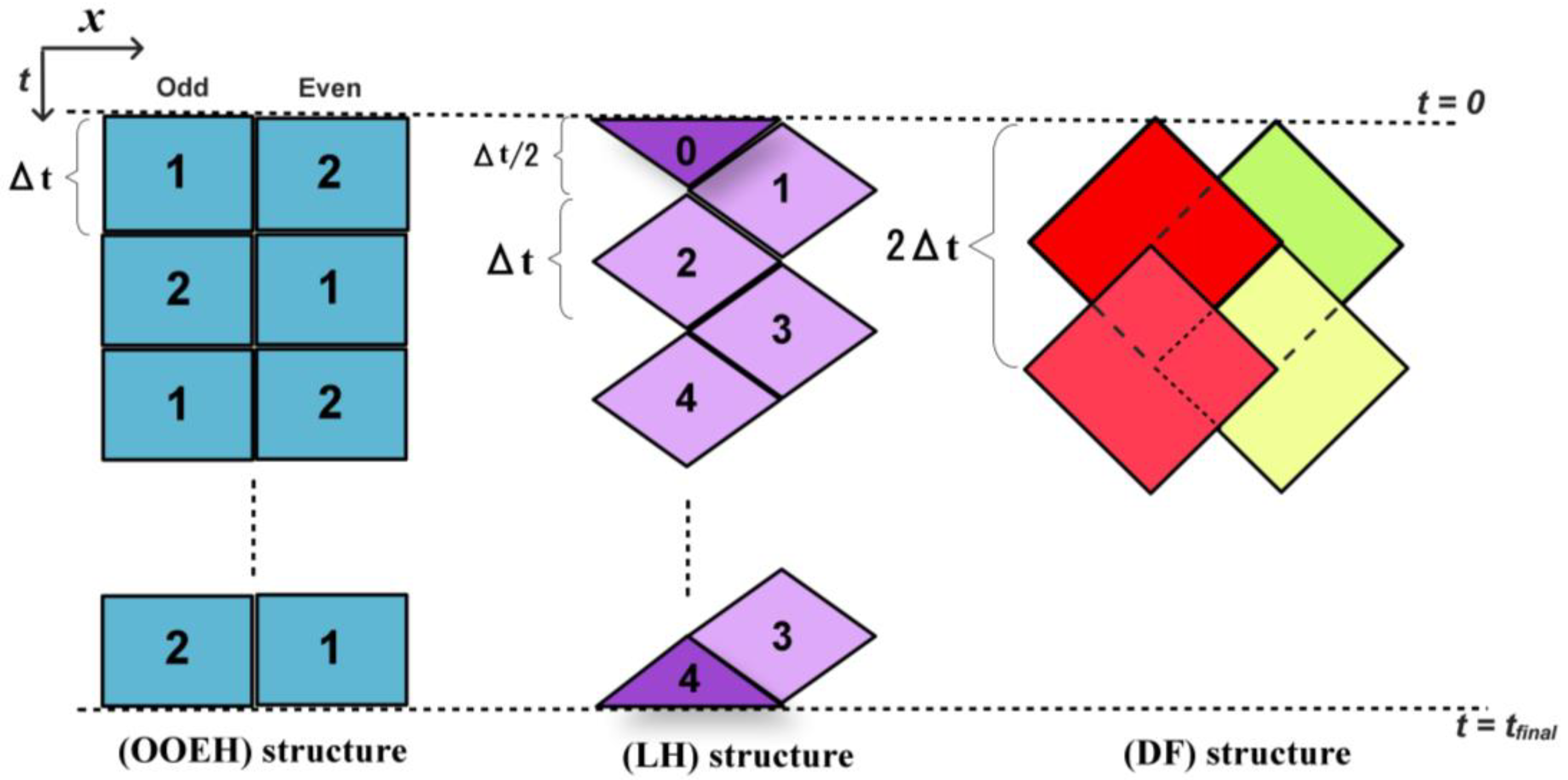
Since the first stage’s time step is halved, the following general formula is applied:
Next, for the even nodes, a full time step is made using
Full time steps, in the same manner, are then taken for the odd and even nodes in turn, where always the most recently obtained values of the neighbors are used to calculate the new values. Lastly, the computations for the odd nodes must be closed using a half-length time step.
According to most of the numerical experiments in our previous works, the LH method is the most efficient among the explicit methods that are unconditionally stable to the linear diffusion equation.
The favorable properties of these algorithms are formulated in the following theorems, which were proved in the original papers.
Theorem 1.
The CCL, OOEH, DF, and LH schemes are unconditionally stable when applied to the spatially discretized linear diffusion equation , which means that the solution is bounded for arbitrary values of α and the time step size.
Theorem 2.
The OOEH, DF, and LH schemes have second-order while the CCL method has third-order convergence when applied to the spatially discretized linear diffusion equation
4. The Incorporation of the Nonlinear Term and Further Methods Used for Comparison
4.1. Operator-Splitting Treatments of the Nonlinear Term
We consider the impact of the Huxley and diffusion terms separately during a time step. We obtain a concentration value after taking into account the diffusion term completely via the diffusion solvers mentioned in the previous subsection, which we briefly represent by for brevity. The form can be used to express the local reaction term. We perform a selective substitution of u by the p values in each of the 12 potential ways:
Each of the obtained expressions is then inserted into the right-hand side of a simple ODE to approximate the time development of u due to the reaction term during the actual time step. In this way, we obtained 12 initial value problems (IVPs), such as
Then, we attempt to solve these IVPs in an analytical way with Maple software. The solution is found in nine cases and not found in three cases, i.e., 4, 5, and 12. During the preliminary numerical tests, we observed that there are five cases (6, 7, 9, 10, and 11) where the scheme does not behave well: the error is large, sometimes due to instabilities. Hence, only the remaining four cases are displayed here in Table 1 and will be used in the remaining part of this paper.

Table 1.
The solutions of the remaining four treatment cases.
When simple operator-splitting is used, a time step begins with the diffusion being treated using one of the algorithms specified in Section 3. Then, as a substitutional step, one of the four procedures (18)–(21) is performed to assess the increment due to the nonlinear term. However, we also apply Strang-splitting, which entails executing one of the processes (18)–(21) once prior to and again subsequent to the computation of the diffusion effect, both with a halved time step size. This indicates that needs to be substituted in (18)–(21) in the first and last stages, and in the first stage, stands instead of in (18)–(21).
Unfortunately, during the preliminary test, we were not able to obtain useful methods when these operator-splitting approaches were combined with the DF scheme. Therefore, only the CCL, OOEH, LH, and (as we will describe later) the CrN diffusion solvers will be combined with the operator-splitting approach.
4.2. Further Treatments of the Nonlinear Term
The following treatments are inspired by our previous work [41], where they were elaborated and applied to the linear reaction (convection) term and the nonlinear radiation term. For further details of the logic of their derivation, the reader should consult that paper. Since the CCL method is a three-stage method with completely different formulas than the OOEH, DF, and LH methods, we were not able to combine it with the following treatments.
- 1.
- Inside treatment.
In this case, the Huxley term is evaluated at the beginning of the actual time step to obtain and inserted during the space and time discretization of the equation. It is multiplied by the time step size h to assess the increment due to the Huxley term. In this approach, the nonlinear term turns up in the numerator of the formulas, as listed below.
- LH method:
- DF scheme:
- OOEH:
- 2.
- Pseudo-implicit treatment (PI).
This case is similar to the previous one, but one of the -s is evaluated at the end of the time step; thus, is inserted instead of . When we rearrange the formula to express , the nonlinear term appears in the denominator as well. The goal of this trick is to enhance stability.
- LH method:
- The Dufort–Frankel (DF):
- OOEH:
- 3.
- Mixed treatment
Mixed treatment means that simply the average of the previous two expressions and is inserted during the discretization. This treatment was proved to be successful in our previous work [41] for the convection term. In this case, we have the following formulas.
- LH method:
- The Dufort–Frankel (DF):
- OOEH:
We note that these treatments will be subjected to intensive numerical tests, but the analytical investigation of the constructed methods is out of the scope of this paper.
4.3. Methods Used for Comparison Purposes
We employ the so-called classical version of the fourth-order Runge–Kutta (RK4) method [42] (p. 737) for comparison’s sake when the running time is measured for large-sized systems. Applying it in the most standard way to our system that is spatially discretized, we have
And, finally,
Along with the RK4, the two-step Adams–Bashforth [43] method (AB2) is also tested in Section 5. As far as we know, the performance of the explicit and stable methods has never been compared to the standard explicit multistep methods.
We will also extensively test an implicit method, which is the widely used Crank–Nicolson (CrN) scheme. It is well known that applying Equation (6) leads to the matrix equation
where I is the unit matrix of size . Since A and B are time-independent in the current work, one can spare running time by calculating prior to the first time step. In this way, only a single matrix multiplication must be performed in each time step: . The CrN method will be combined with the simple and Strang operator-splitting treatments of the nonlinear term listed in Section 4.1.
The next set of methods belongs to the family of the nonstandard finite difference methods. They are developed to solve nonlinear PDE (1) in one space dimension with and using an equidistant mesh. Four nonstandard finite difference techniques using the following formulas were proposed in paper [3]:
where , , , and . The positivity and boundedness of these schemes have been analytically shown. These are not, however, unconditional; the most crucial condition is , which is similar to the typical CFL limit for the explicit Euler method.
When we perform running time measurements in large 2D systems, we also employ ode15s for comparison purposes. This solver is included in MATLAB, where 15s means a one- to five-order numerical differentiation formula with variable step and variable order (VSVO) that was designed for stiff problems.
5. First Round of Numerical Experiments: Verification and Selection Based on Errors
The following formula is used to compare the numerical solutions generated by the solver under examination with the analytical reference solution at the final time in order to determine the maximum numerical errors:
The average error is also very similar:
We refer to the third kind of error as the energy error as it has an energy dimension in the context of the heat conduction equation:
As we already mentioned, our goal is to assess the performance of the methods not only for one concrete time step size but for many. Hence, starting from a very large time step size, we calculate the above-defined errors for a series of decreasing time step sizes. This series of time step sizes usually starts from T/4 and has S elements, where the next element is obtained by taking half of the previous one. Then, we compute the three kinds of aggregated error, , , and , as the mean of the logarithm of these errors as follows:
Finally, the average of the three different AgErr errors is determined:
and this Agerr quantity is used to evaluate the overall accuracy for the small, medium, and large time step sizes for many possible combinations. It should be noted that the method is very accurate when AgErr is negative and has a big absolute value. In the case of instabilities, the u values can be too large for MATLAB to handle, and ‘NaN’ symbols appear instead of numbers. In these cases, the error is substituted by 1010 as a penalty for unstable behavior. This ensures that the aggregated errors are numbers that can be comparable to other errors.
5.1. Experiment 1: One Space Dimension Using an Exact Solution
In this and the following experiment, PDE (1) with will be solved on the domain . The following analytical solution [1] (p. 34) serves as the reference for validation.
By evaluating this function at the time and space locations that correspond to the initial time and the boundaries , respectively, the initial and Dirichlet boundary conditions are determined.
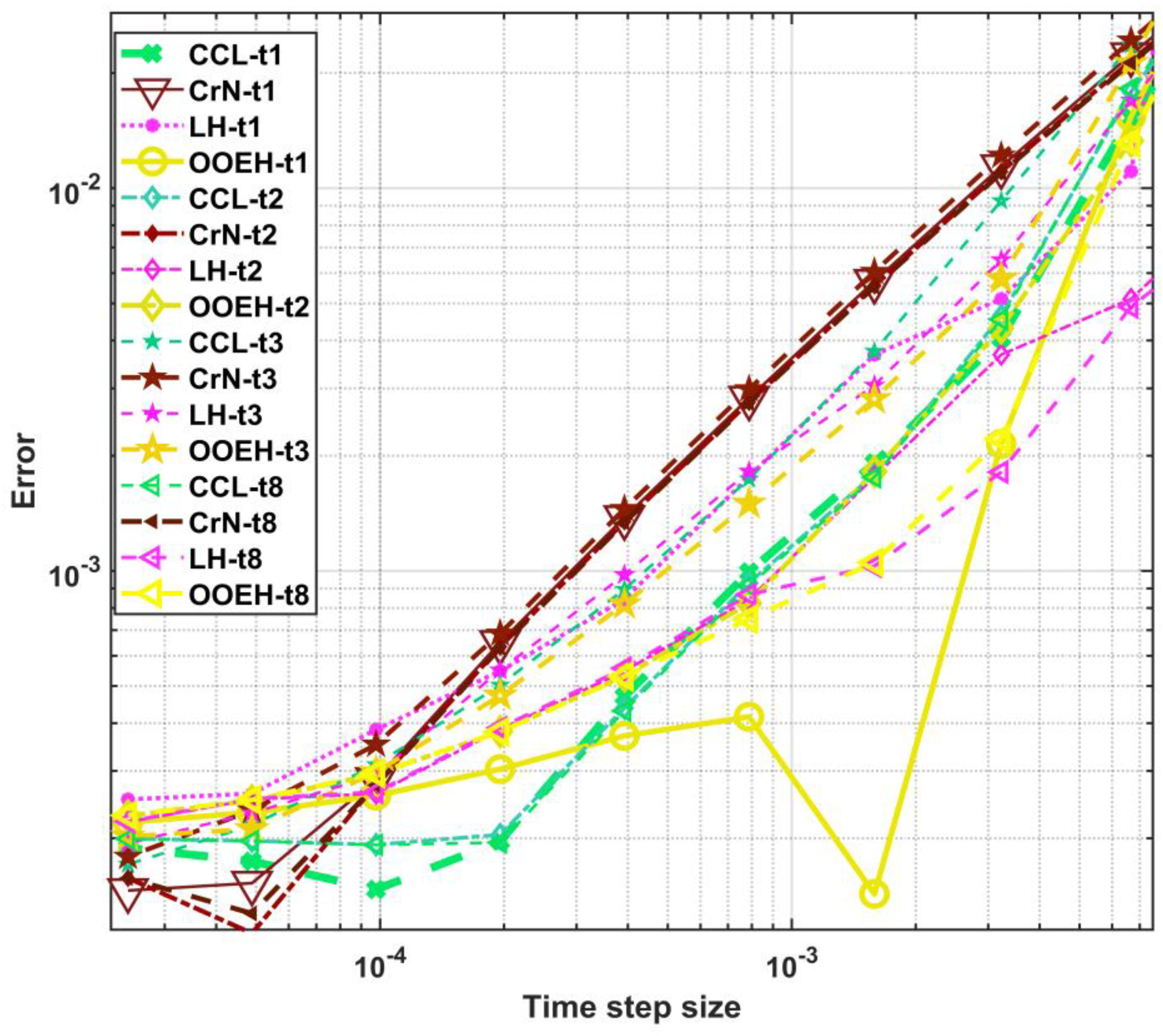
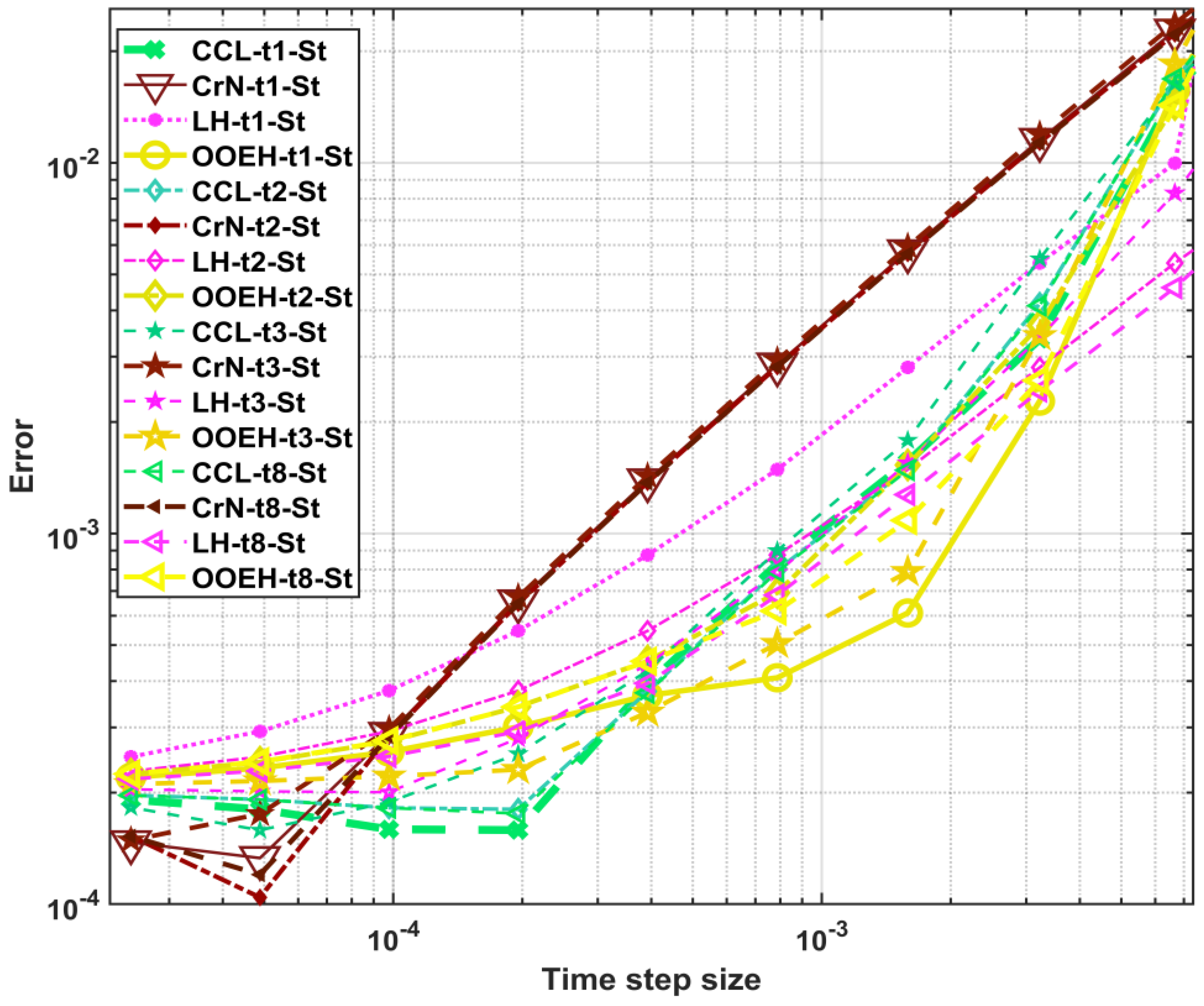
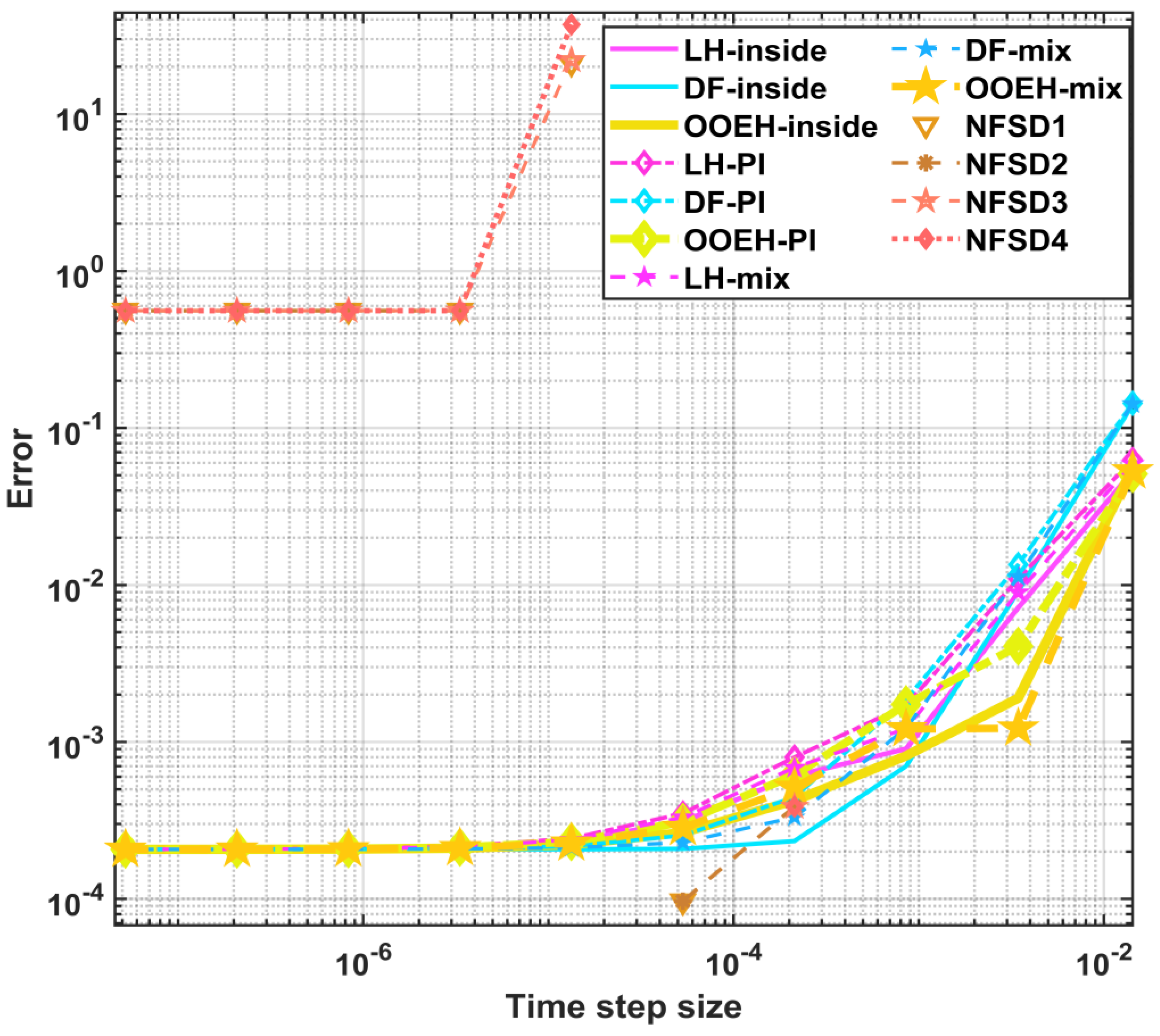
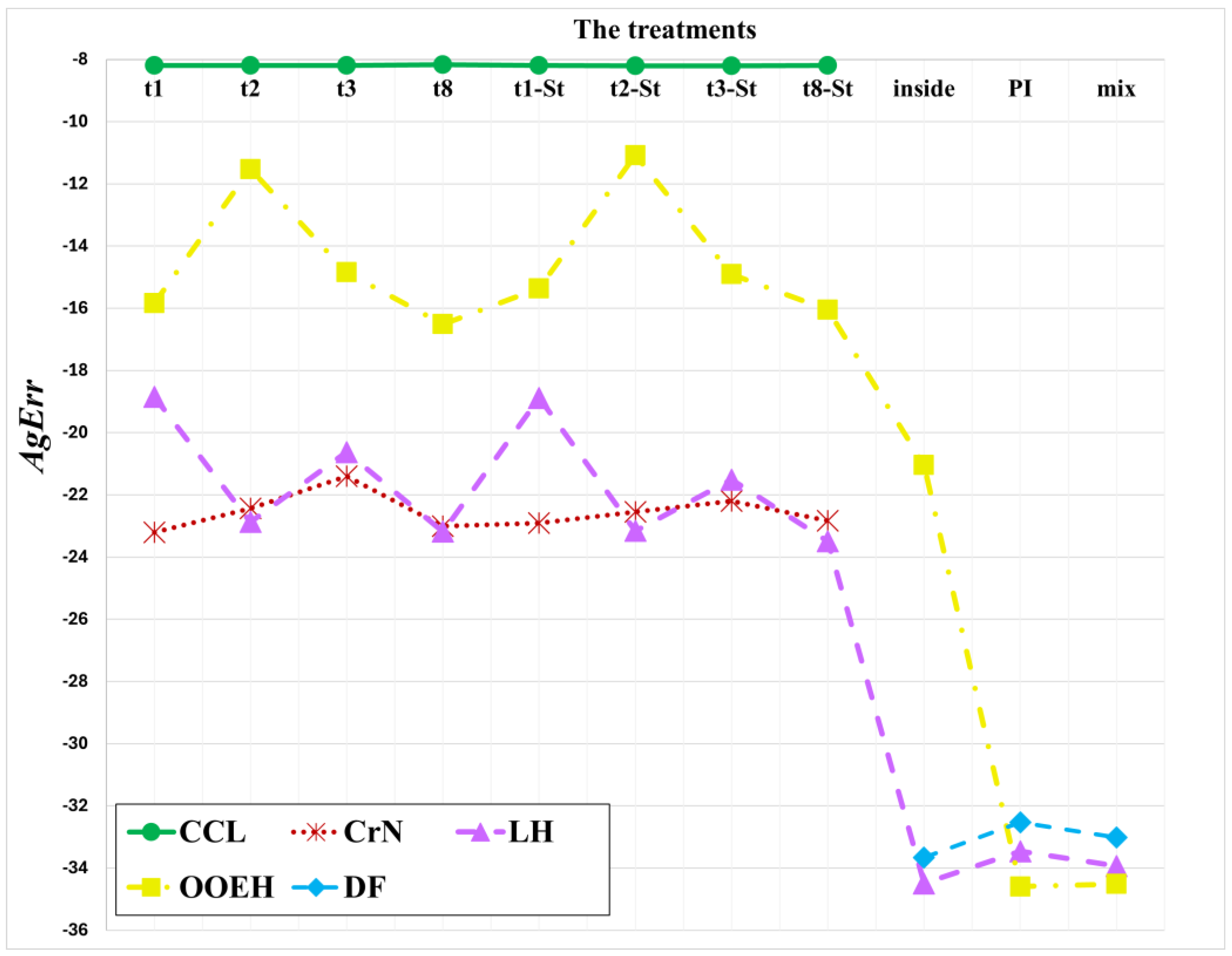
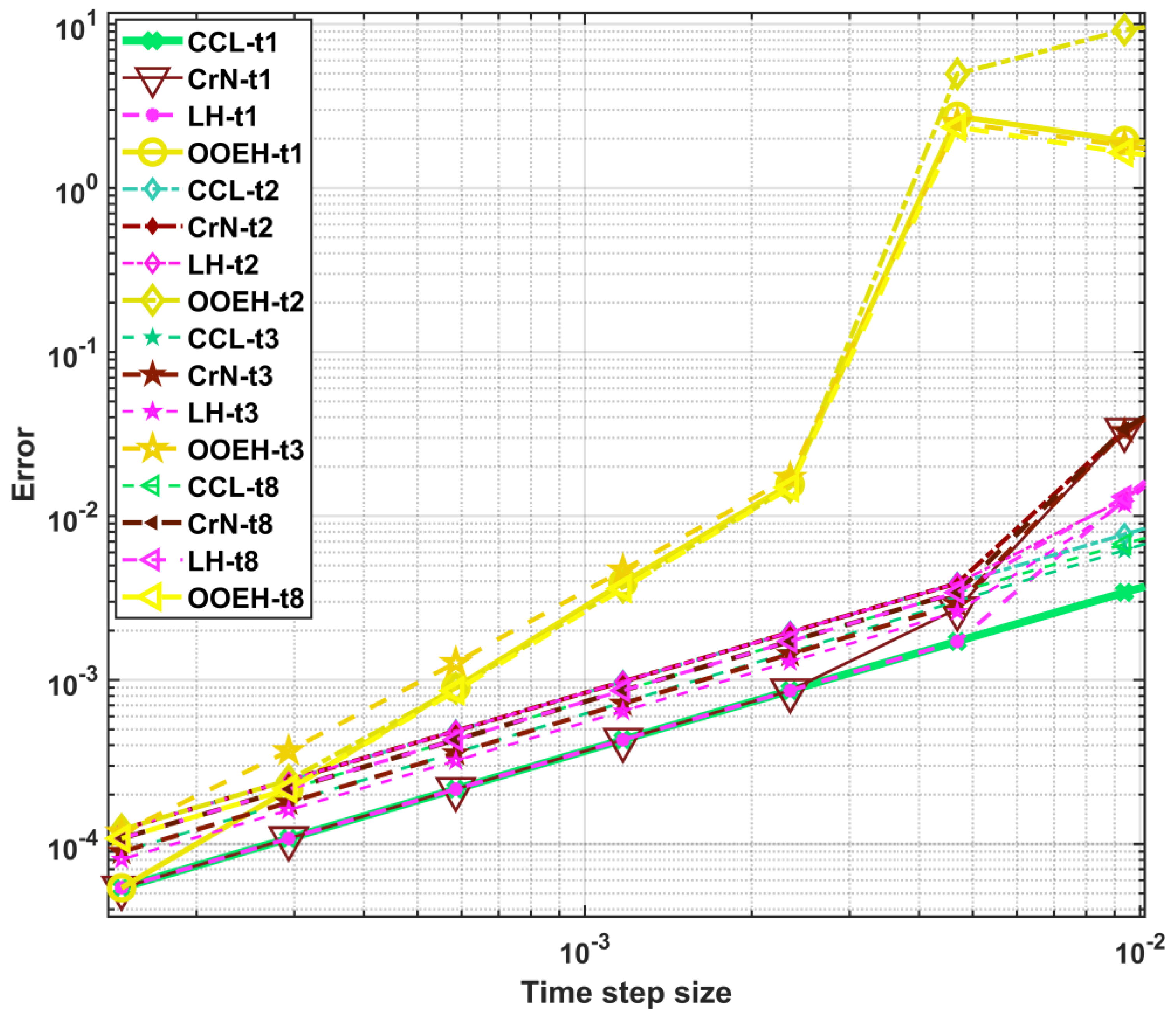
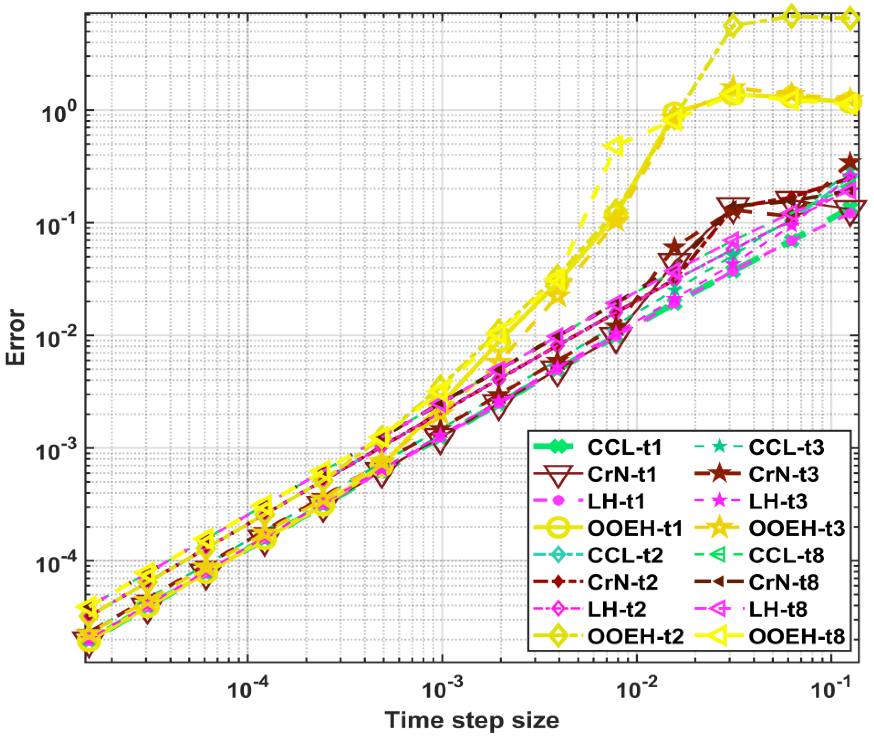
In Experiment 1, , and the space step size ∆x = 0.004. The nonlinear coefficient is , and c = 19 in Equation (43). Figure 2, Figure 3 and Figure 4 show the maximum errors as a function of time step size for different method combinations. The aggregated errors for different diffusion solvers and treatments of the Huxley term are shown in Figure 5 and Table 2. Since the errors go down with the time step size, the methods can be considered verified.

Figure 2.
Maximum errors as a function of time step size h for different operator-splitting treatments in the case of Experiment 1.
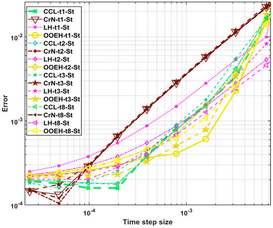
Figure 3.
Maximum errors as a function of time step size for different operator-splitting treatments with Strang-splitting in the case of Experiment 1.
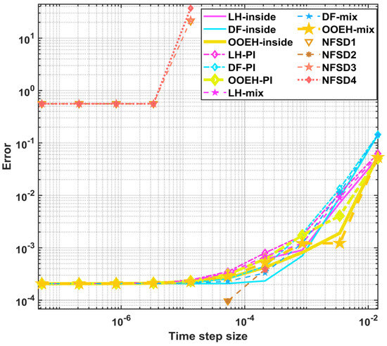
Figure 4.
Maximum errors as a function of time step size for the remaining methods in the case of Experiment 1.
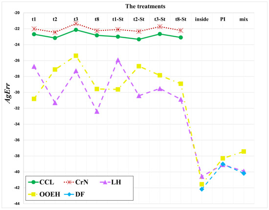
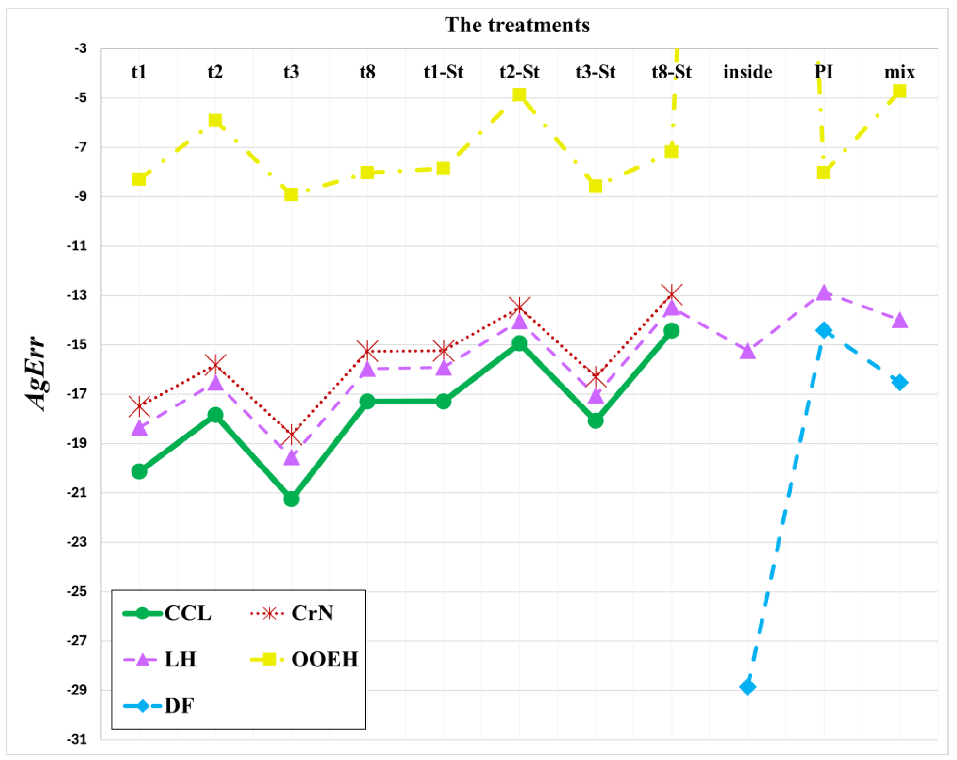
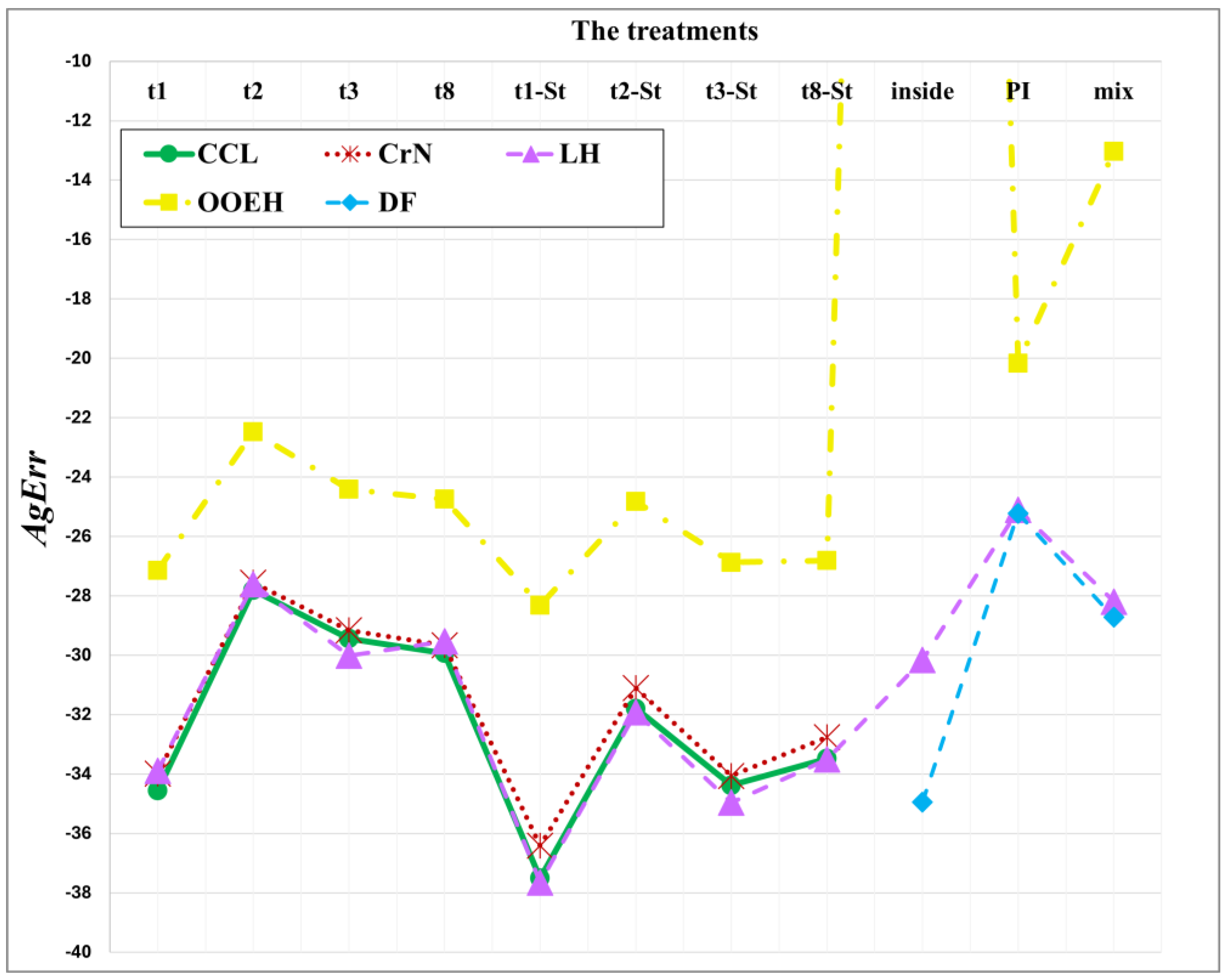
Figure 5.
The aggregated errors (AgErr) for different diffusion solvers and treatments of the Huxley term in the case of Experiment 1.
Table 2.
The aggregated error (AgErr) values for different treatment of the methods in the case of Experiment 1.
5.2. Experiment 2: One Space Dimension Using an Exact Solution, Larger Final Time
Here, PDE (1) is discretized on the domain using the space step size ∆x = 0.005, . The nonlinear coefficient is and c = 179 in Equation (43). The aggregated errors for different diffusion solvers and treatments of the Huxley term are shown in Figure 6 and Table 3. The maximum errors as a function of time step size for different method combinations are presented in the Supplementary Materials (see Figures S1–S3).

Figure 6.
Aggregated errors (AgErr) for different diffusion solvers and treatments of the Huxley term in the case of Experiment 2.
Table 3.
The aggregated error (AgErr) values for different treatment of the methods in the case of Experiment 2.
The main conclusion of the first two experiments is that the operator-splitting treatments yield larger errors than the other (inside, PI, and mixed) treatments, with the exception of OOEH–inside. The NSFD schemes sometimes give very small errors, but they are completely unreliable. Since the systems are not stiff here, the implicit CrN method has no advantage compared to the other methods.
5.3. Experiment 3: Stiff 2D System
Employing the capacity–resistivity model described in Section 2, we have two space dimensions from this point. Using a log-uniform distribution, we produce random values for the resistances and capacities as follows:
We create highly varied test problems by changing the a and b values. The variable rand is MATLAB-generated random numbers within the unit interval. From this point, the reference solution is provided by the ode15s solver of MATLAB with a very stringent tolerance (10−11) to ensure accuracy. The used mesh size and final time are while and . These variables give and . The initial concentration function is the sum of a smooth function and some random numbers:
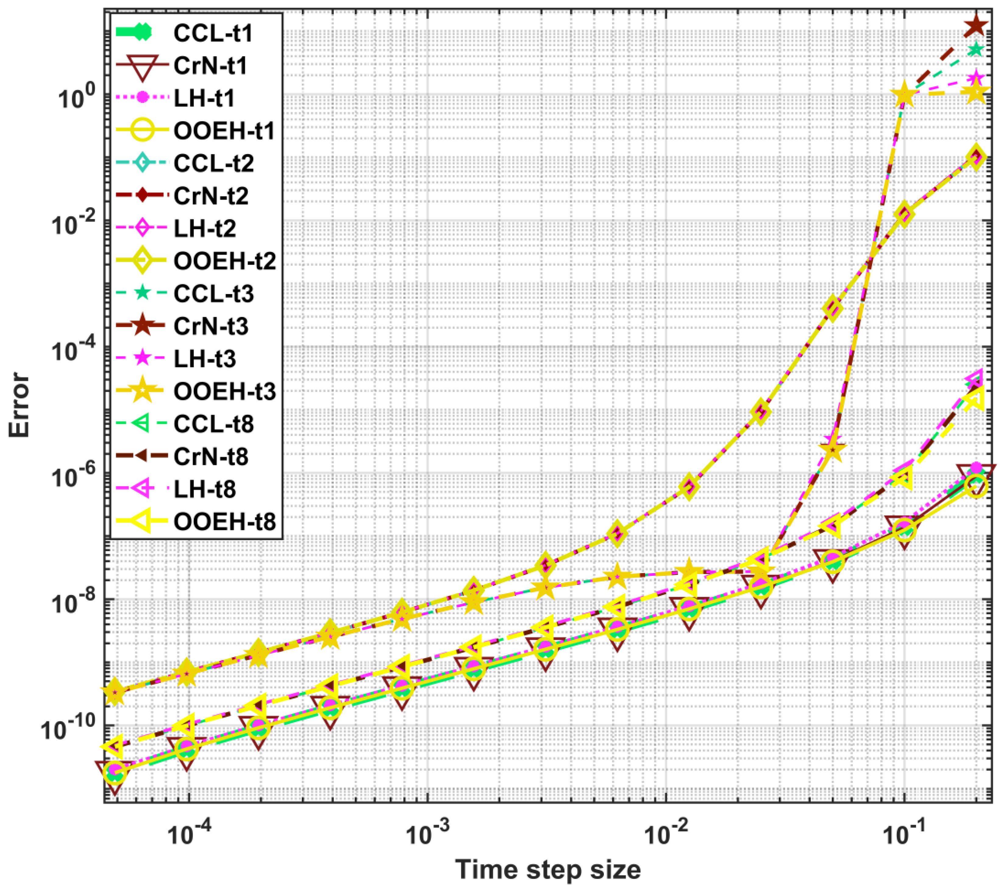
Figure 7 and Figure 8 show the maximum errors as a function of time step size for different method combinations. The maximum errors for different operator-splitting treatments with Strang-splitting are presented in the Supplementary Materials (Figure S4). The aggregated errors for different diffusion solvers and treatments of the Huxley term are presented in Figure 9 and Table 4.
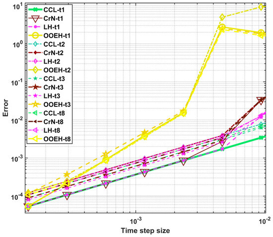
Figure 7.
Maximum errors as a function of time step size for different operator-splitting treatments in the case of Experiment 3.
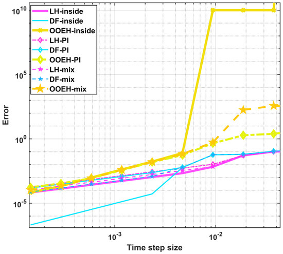
Figure 8.
Maximum errors as a function of time step size for the remaining methods in the case of Experiment 3.
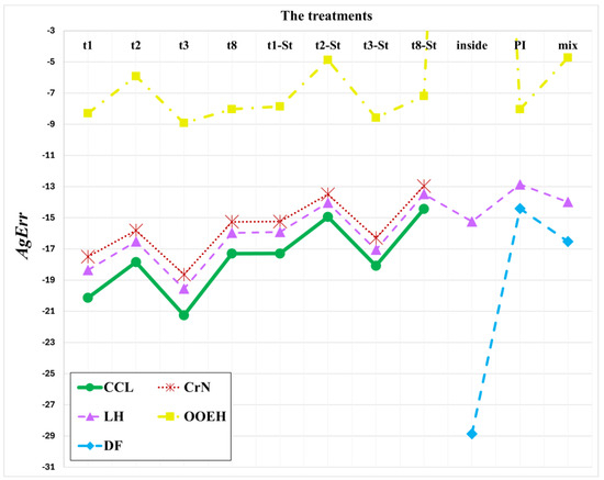
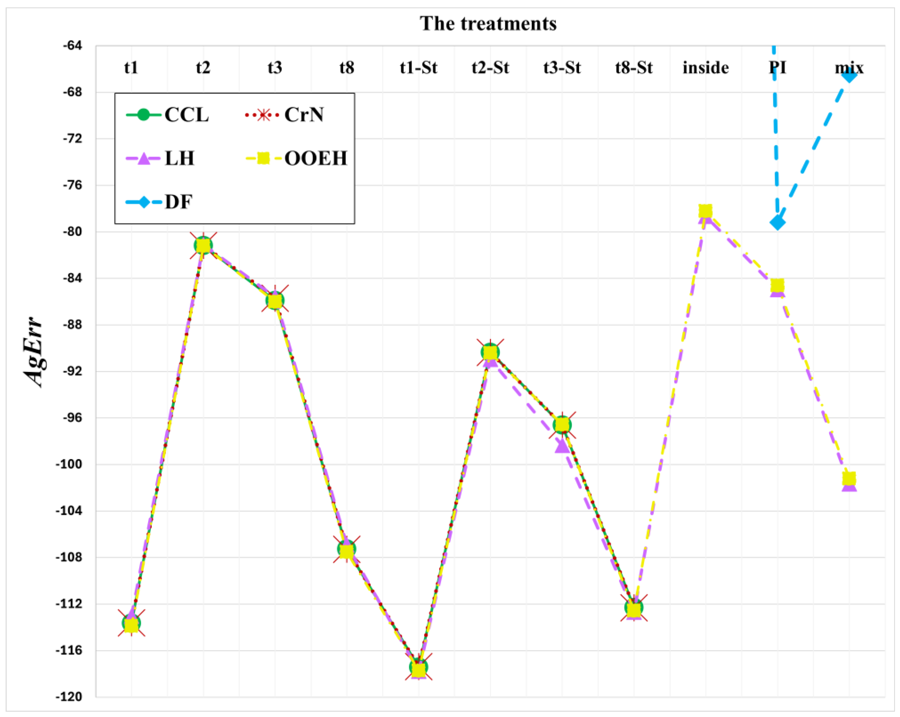
Figure 9.
The aggregated errors (AgErr) for different diffusion solvers and treatments of the Huxley term in the case of Experiment 3.
Table 4.
The aggregated error (AgErr) values for different treatment of the methods in the case of Experiment 3.
One can see that the DF–inside combination shows the best performance since its convergence rate is the highest. On the other hand, the operator-splitting treatments behave much better than before, especially the t1, t3, and t3-Strang treatments.
5.4. Experiment 4: Non-Stiff System with Strong Nonlinearity
The used mesh size and final time are while , and . These variables give and . The random component in the initial concentration function is slightly larger than before:
Figure 10 shows the maximum errors as a function of time step size for different operator-splitting treatments. These errors for different operator-splitting treatments with Strang-splitting and for the remaining methods are presented in the Supplementary Materials (see Figures S5 and S6). The aggregated errors for different diffusion solvers and treatments of the Huxley term are shown in Figure 11 and Table 5. The results show that in this case, the treatment of the nonlinear term is much more important than that of the diffusion term. This is logical since the coefficient is large, while the problem is easy to solve from the point of view of diffusion. The large value of has another consequence: the “force” acting on u towards its maximum value 1 is large. Since the final time is also quite large, the values of u are getting very close to 1. When this happens, the importance of the diffusion process decreases, which further reinforces the previously mentioned effect and decreases the calculation errors below 10−10 for short time step sizes. The DF–inside method, which was the most accurate in the previous experiment, is unstable here for almost all time step sizes, and that is why its error is large.
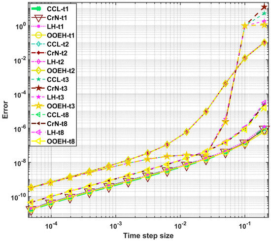
Figure 10.
Maximum errors as a function of time step size for different operator-splitting treatments in the case of Experiment 4.
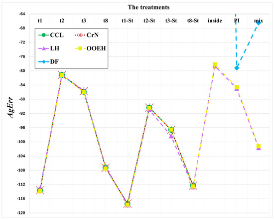
Figure 11.
The aggregated errors (AgErr) for different diffusion solvers and treatments of the Huxley term in the case of Experiment 4.
Table 5.
The aggregated error (AgErr) values for different treatment of the methods in the case of Experiment 4.
5.5. Experiment 5: Medium Stiffness and Nonlinear Coefficient
The used mesh size and final time are while , and . These variables give and . The initial concentration function is:
Figure 12 shows the maximum errors as a function of time step size for different operator-splitting treatments. The maximum errors as a function of time step size for different operator-splitting treatments with Strang-splitting and for the remaining methods are presented in the Supplementary Materials (see Figures S7 and S8). The aggregated errors for different diffusion solvers and treatments of the Huxley are presented in Figure 13 and Table 6.
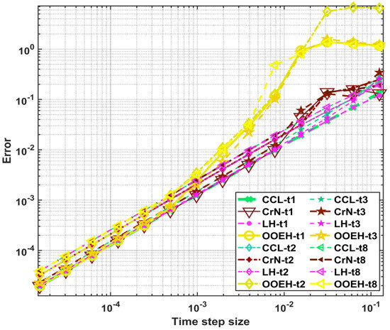
Figure 12.
Maximum errors as a function of time step size for different operator-splitting treatments in the case of Experiment 5.

Figure 13.
The aggregated errors (AgErr) for different diffusion solvers and treatments of the Huxley term in the case of Experiment 5.
Table 6.
The Aggregated error (AgErr) values for different treatment of the methods in the case of Experiment 5.
5.6. The Summary of the Five Experiments
The simple sum of the aggregated errors for different diffusion solvers and treatments of the Huxley term are shown in Figure 14 and Table 7. Based on these results, we select the following 15 methods for further examination: LH-t1, LH-t1-Strang, LH-t3-Strang, LH-t8-Strang, LH–inside, LH-mix, DF-PI, DF–mixed, OOEH-PI, OOEH-t8-Strang, CCL-t1, CCL-t1-Strang, CCL-t8-Strang, CrN-t1, and CrN-t1-Strang. We note that since simple operator-splitting is calculated faster than Strang-splitting, we are slightly biased towards the simple splitting to give them a further chance in the next section, where running time will be measured.
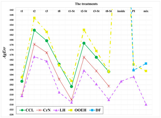
Figure 14.
The aggregated errors (AgErr) for different diffusion solvers and treatments of the Huxley term.
Table 7.
The aggregated errors (AgErr) for different treatment of the methods.
6. Second Round of Numerical Experiments: Selection by the Performance with Running Time Measurements in 2D
6.1. Experiment 6: Non-Stiff System
In this section, the systems are much larger to make running time measurements meaningful. Here, the used system size is In order to create a system with a relatively low stiffness ratio, we set , which is equivalent to a uniform mesh with constant α. These parameters yield , . Meanwhile, the final time is , while the coefficient of the reaction term is . The initial concentration is given by the continuous function:
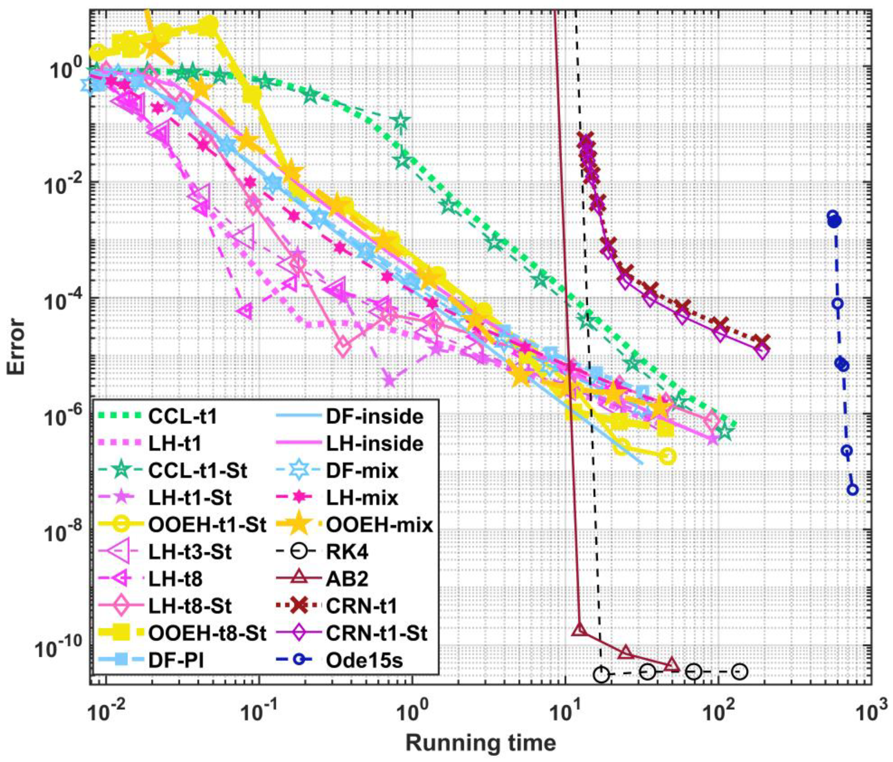
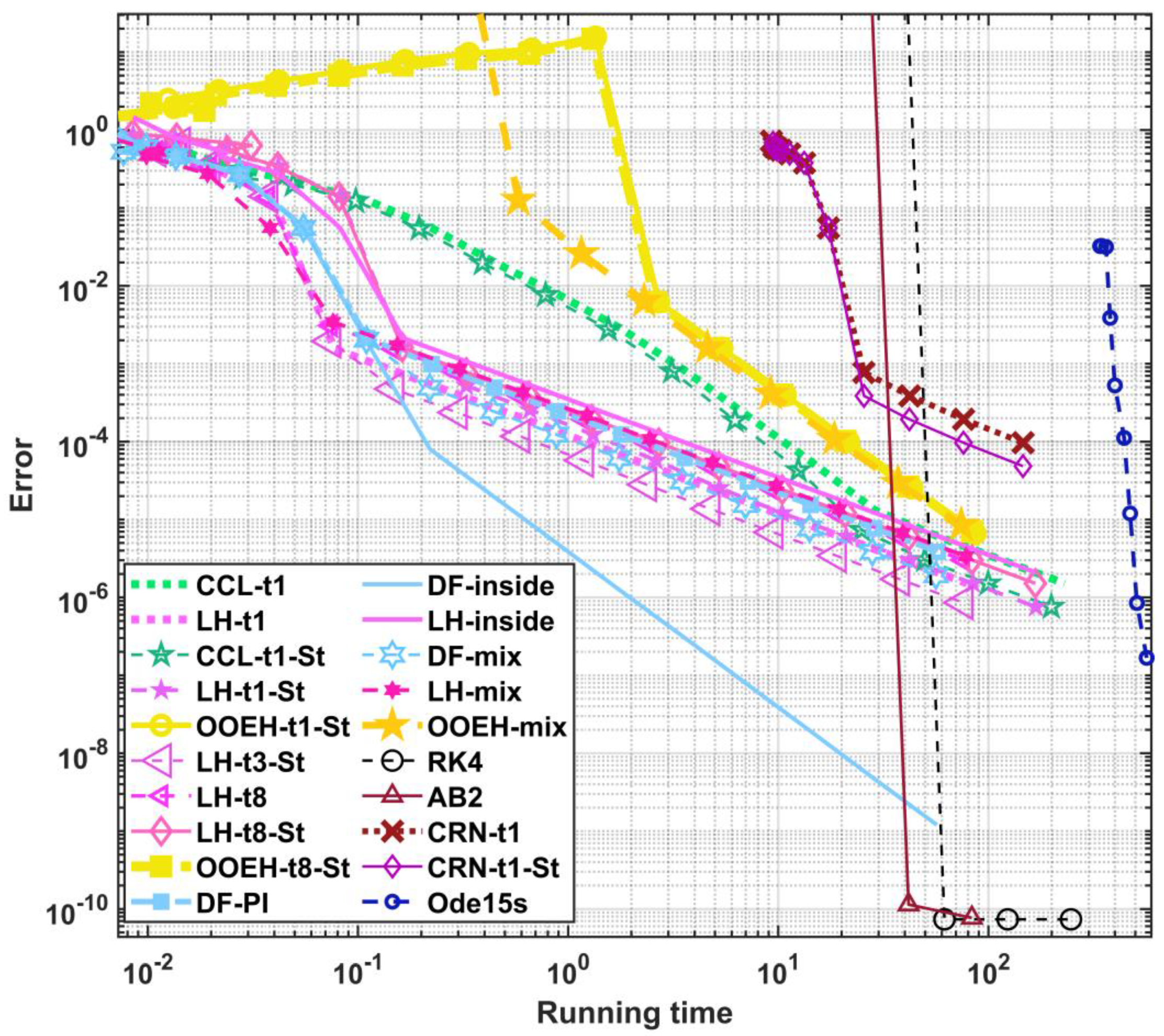
The tic-toc function in MATLAB is used to measure the running times. All the running times are measured on a desktop computer with an Intel Core i7-13700 (24 CPUs) and 64 GB RAM is used. The calculations are completed more than one time; then, the average running times are determined to reduce the impact of the random fluctuations. The obtained maximum errors are shown as a function of the running times in Figure 15. One can see from the figure the LH-t1, LH-t1-Strang, and LH-t8-Strang methods are more efficient than other methods when low or medium accuracy is required. The solvers RK4 and ode15s provide extremely high accuracy but with longer computation time. The aggregated errors for different methods in Experiment 6 are presented in the Supplementary Materials (see Table S1).
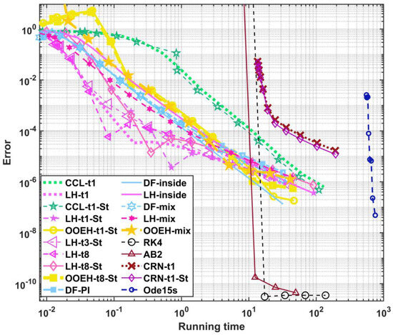
Figure 15.
Maximum errors as a function of the running time for Experiment 6; non-stiff system.
6.2. Experiment 7: Moderately Stiff System
In this case, the system size and the final time used are , and , while the exponents are . These variables give and . This indicates that the system is moderately stiff only. The initial concentrations contain random numbers in the unit interval as follows:
In Figure 16, we show the errors as a function of running times. The aggregated errors for different treatments of the methods in the case of Experiment 7 are presented in the Supplementary Materials (see Table S2). One can see when the stiffness increases, the LH-t3-Strang method is the most efficient, closely followed by LH-t1, CCL-t1-Strang, LH-t1-Strang, LH-t8-Strang, OOEH-t3-Strang, and DF-mix.

Figure 16.
Maximum errors as a function of the running time for Experiment 7; moderately stiff system.
6.3. Experiment 8: Very Stiff System
Now, the used system size is and the exponents are . These parameters provide the values and , which means that the system is rather very stiff. The final time is , and the coefficient of the reaction term is . The initial concentrations also contain random numbers in the unit interval:
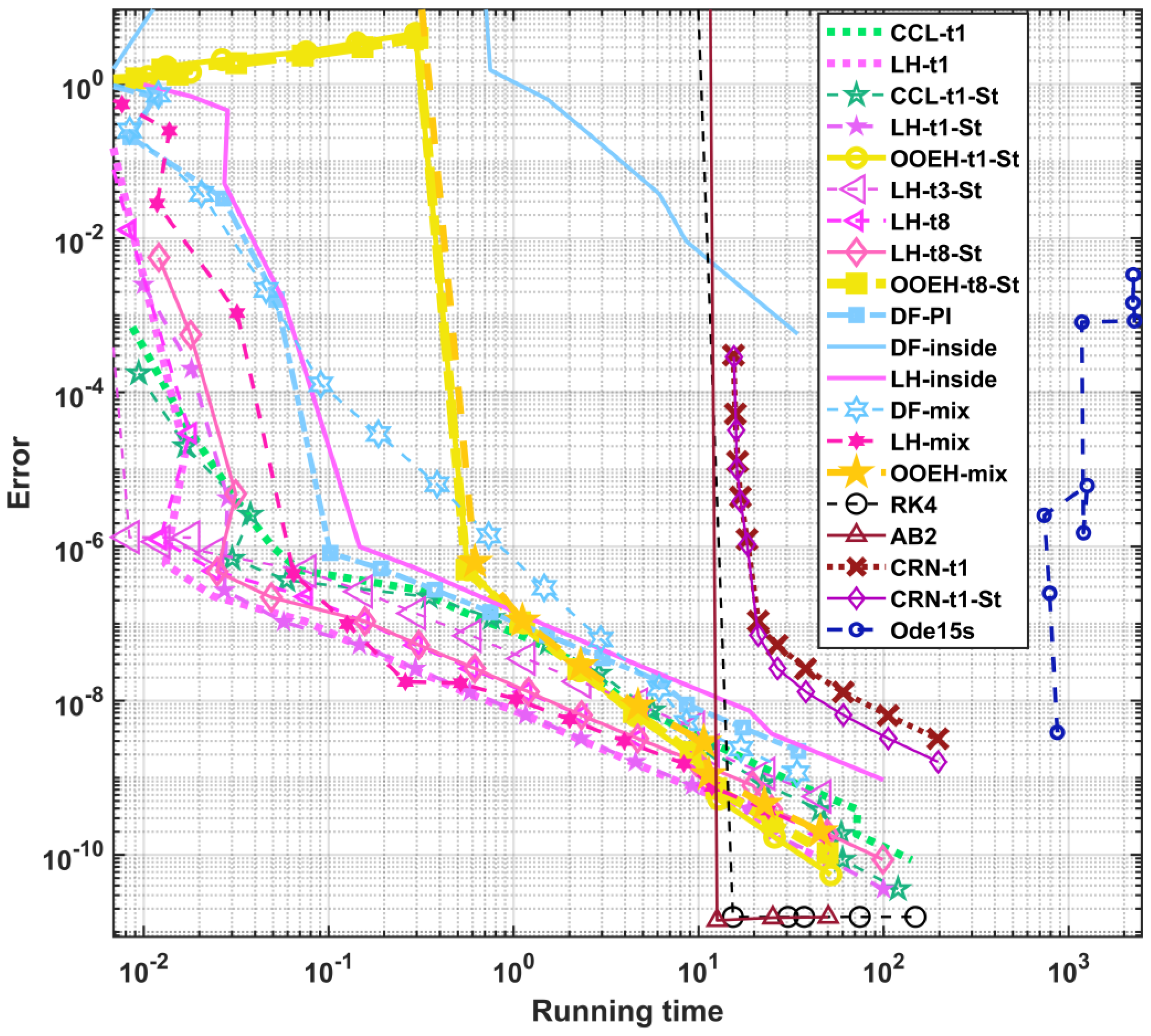
In Figure 17, we present the maximum errors as a function of the running times. The aggregated errors for different treatments of the methods in the case of Experiment 8 are presented in the Supplementary Materials (see Table S3).
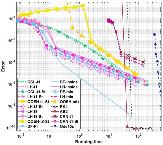
Figure 17.
Maximum errors as a function of the running time for Experiment 8; very stiff system.
Based on these and the previous experiments, we choose the top seven methods to include the following combinations: LH-t1, LH-t1-Strang, LH-t3-Strang, LH-t8-Strang, CCL-t1-Strang, OOEH-t8-Strang and DF–mixed.
7. Third Round of Numerical Experiments: Parameter Sweep for the Top Seven Methods
7.1. Experiment 9: Sweep for the Size of Capacities and Resistances
The used system size and final time are while and . Let us simulate a system that consists of two homogeneous parts. In the second half, the material properties are different, which is reflected by smaller capacities and the resistances. We assume
where . This means we first run the simulation using the first value of , register the errors, decrease to 0.3 without changing any other parameters, run the code again, etc. The initial concentration function is a smooth function as follows:
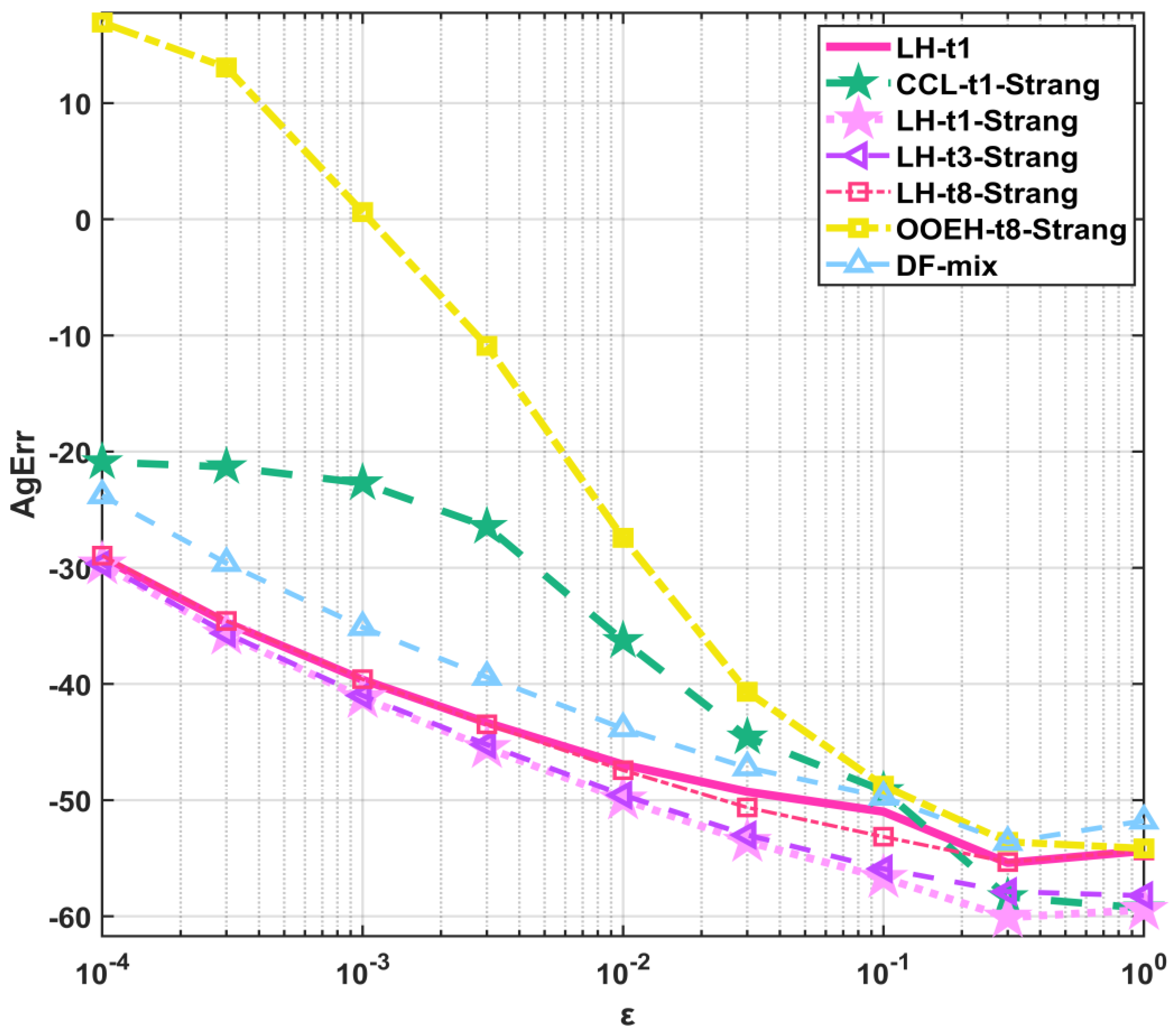
If the capacities and resistances are decreasing, the physical process of diffusion becomes faster. To follow these faster changes, a shorter time step size should be used due to the decreasing CFL limit. However, we keep the set of the used time step sizes fixed; therefore, we experience an increase in the errors with decreasing . The interesting fact is that this increase is very different for the different methods: the worst is for the OOEH method and much less for the other methods. In Figure 18 and Table 8, we present the aggregated errors as a function of the ε in the case of Experiment 9 for the top seven methods. One can see that with the exception of the original hopscotch method, the algorithms perform well even in the case where the CFL limits for the explicit RK methods are extremely low.

Figure 18.
Aggregated errors (AgErr) as a function of the ε in the case of Experiment 9 for the top 7 methods.
Table 8.
Aggregated errors (AgErr) for different (ε) values of the top 7 methods.
7.2. Experiment 10: Sweep for the Stiffness Ratio
Now, in this section, we can add a new parameter γ to generate a wide scale of random values for the C and R quantities as follows:
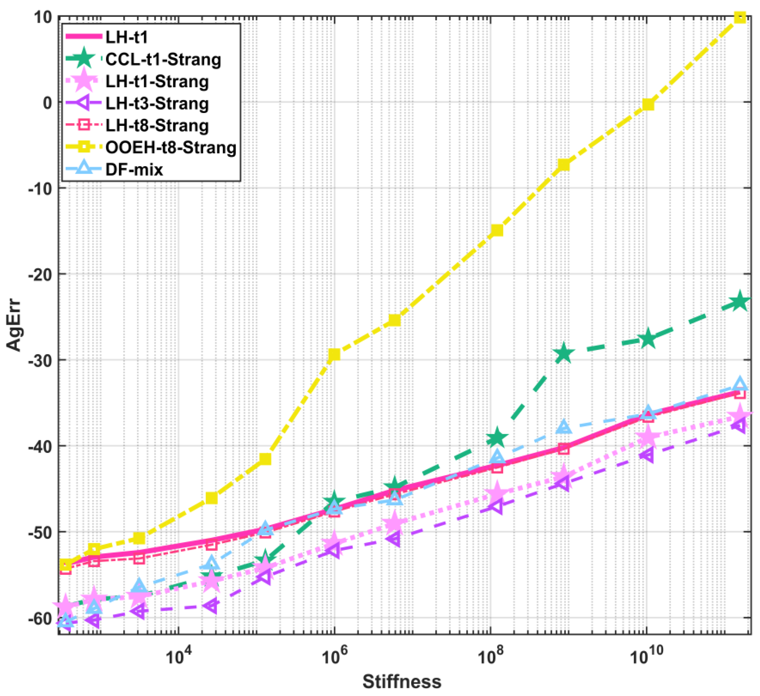
where . The used final time is , the system size is and , while The initial concentration function is as follows: . The aggregated errors as a function of the stiffness ratio in the case of Experiment 10 for the top seven methods are shown in Figure 19 and Table 9.
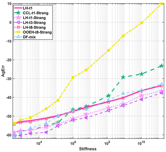
Figure 19.
Aggregated errors (AgErr) as a function of the stiffness ratio (SR) in the case of Experiment 10 for the top 7 methods.
Table 9.
Stiffness ratio (SR), CFL limit (CFL), and aggregated error (AgErr) values for different values of gamma (γ) and different treatments of the top 7 methods.
This experiment reinforces that it is generally true that the performance of the OOEH algorithm declines much more severely with a decreasing CFL limit and increasing stiffness than the other methods. From these two experiments, one could conclude that this statement, albeit to a much lower extent, is true for the CCL method. However, this would be a hasty judgement since, in Experiment 3, increased stiffness resulted in a relative advantage for the CCL method.
7.3. Experiment 11: Sweep for the Nonlinear Coefficient β
In this case, we use the coefficient of the Huxley term β, where the system size and final time are , and , while the exponents are . The initial concentration function is given as . In this experiment, however, a problem arises when the value of β is large. In these cases, the values of the u function are forced to approach unity very closely due to the Huxley term, which is always positive for u values in the unit interval. Hence, a method can be accidentally accurate if it yields the function, which is the only equilibrium point of the equation. This distorts the results and the evaluation of the performance of the methods. To avoid this, we change the boundary conditions in two points of the system to . This means that we apply fixed Dirichlet boundary conditions, but only for these two cells; the other boundaries are still subjected to zero-Neumann b.c.-s. This is implemented by modifying the loop for the cells from i = 1:N to i = 2:(N-1).
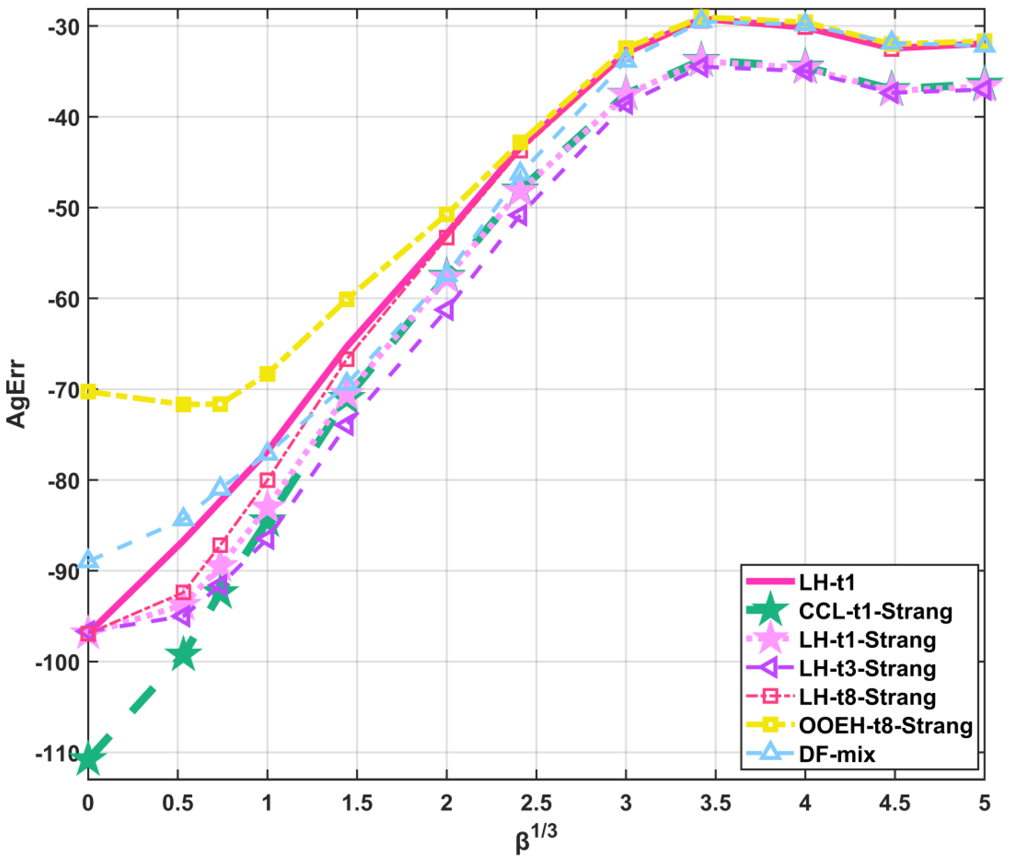
In Figure 20 and Table 10, we present the aggregated errors as a function of the third root of the β parameter for the top seven methods. One can see that the initially significant differences between the methods almost vanish with increasing β, and two groups of the methods appear. The group with the smaller error always uses the t1-Strang or t3-Strang treatments, and the rest of the treatments constitute the other group. Nevertheless, the difference between these two groups is quite small. One can also observe that the initial disadvantage of the OOEH method (which is due to the moderate stiffness of the problem) vanishes because, for large values of β, the treatment of the nonlinear term is much more important than that of the diffusion term.

Figure 20.
Aggregated errors (AgErr) as a function of parameter β in the case of Experiment 11 for the top 7 methods.
Table 10.
Aggregated errors (AgErr) for different β values of the top 7 methods.
7.4. Experiment 12: Sweep for the Final Time T
In this case, we gradually increase the final time, i.e., , while the system with all of its parameters is kept fixed. The used system size is , , while . The exponents are . The initial concentration function is given as:
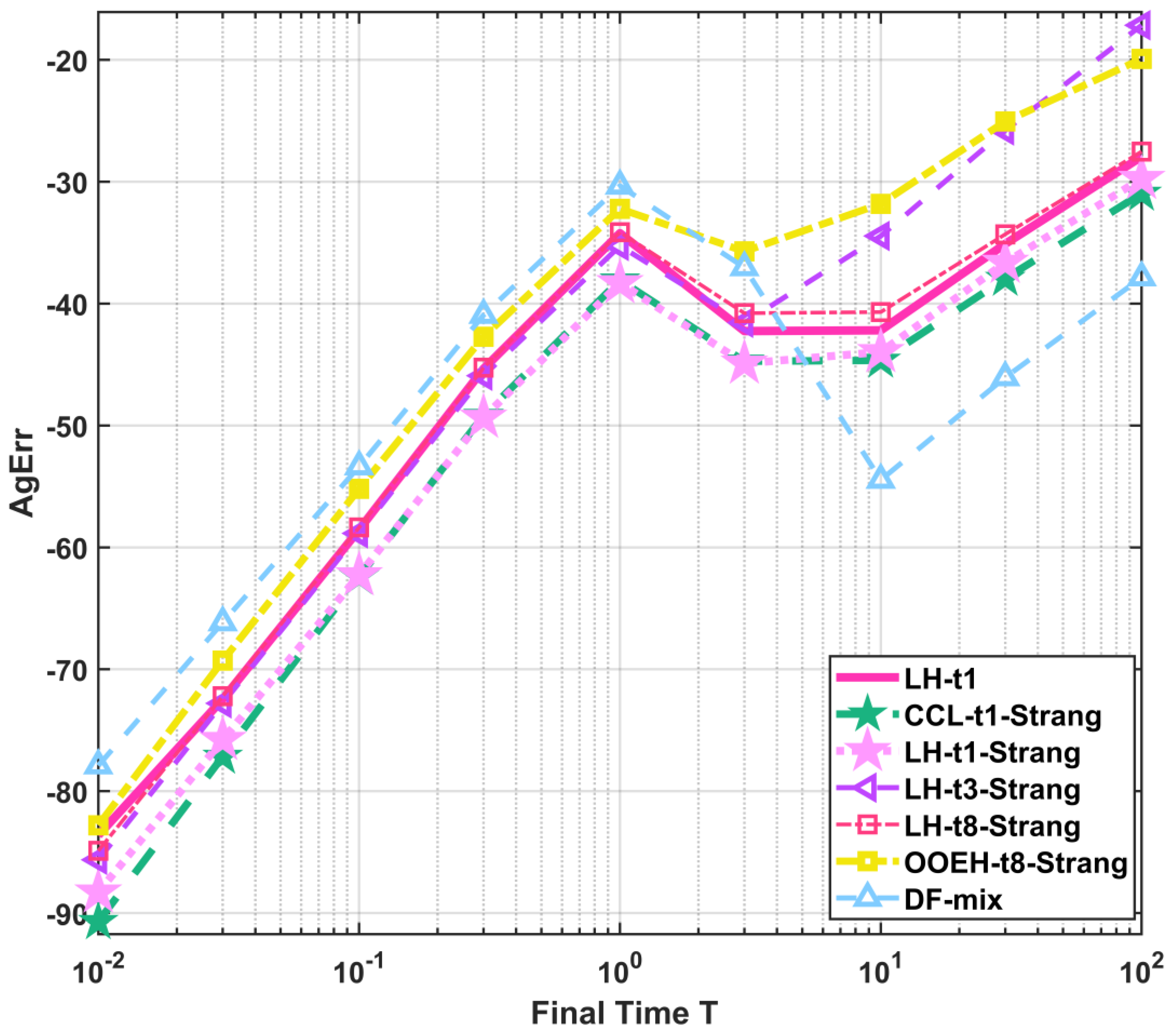
Since for large final times, the u values become very close to 1, as in the previous example for large values of β, we apply the same boundary conditions as in Experiment 11. Moreover, the series of time step sizes start from T/4; thus, the set of the used time step sizes is shifted with the final times. This choice, which is made to avoid extremely long running times, yields gradually increasing aggregated errors for most of the methods. Figure 21 and Table 11 show the aggregated errors as a function of the final time T in the case of Experiment 12 for the top seven methods. One can see that when T exceeds 1, there is a temporary decrease in the aggregated errors. This is because, by this time, the simulated system approached the stationary state very closely, and, therefore, the fine differences in the transient simulation by the different methods decay. The maximum errors as a function of time step size for T = 100 in the case of Experiment 13 for the top seven methods are presented in the Supplementary Materials (see Figure S9). One can conclude that the DF scheme has a relative advantage when the task is to approach accurately the stationary states.

Figure 21.
Aggregated errors (AgErr) as a function of the time in the case of Experiment 12 for the top 7 methods.
Table 11.
Aggregated errors (AgErr) for different time values of the top 7 methods.
7.5. Experiment 13: Sweep for the Initial Function Wavelength
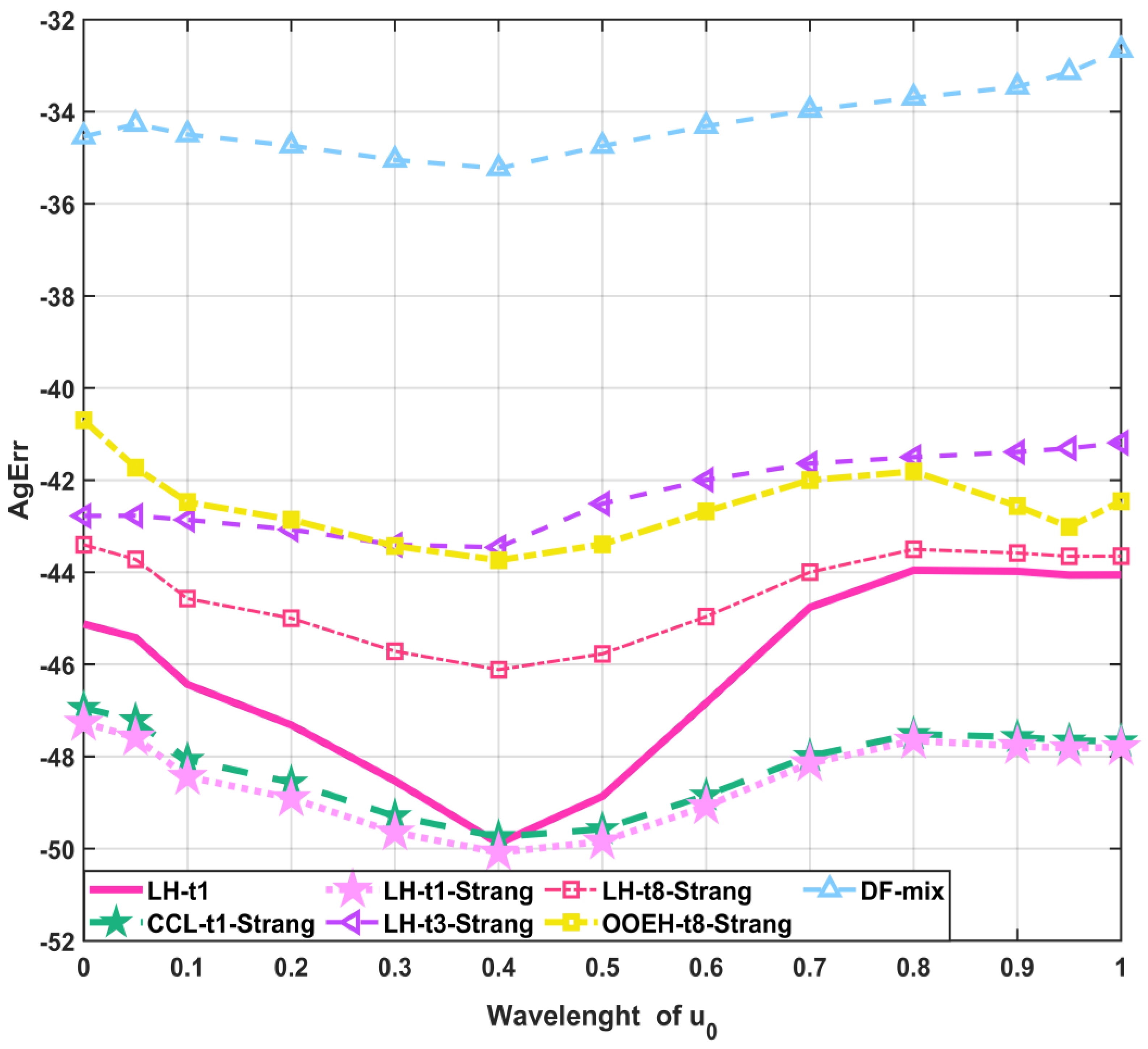
The parameters of this experiment are the following: , , . The initial concentration function is a sum of the components. Here, and for the rest of this paper, we return back to fully zero-Neumann b. c.-s. The first component with weight w is a smooth long-wave cosine function, while the second component with weight 1-w is the shortest possible wavelength function:
where .
Figure 22 and Table 12 show the aggregated errors as a function of w in the case of Experiment 12 for the top seven methods. The maximum errors as a function of the time step size for w = 1 in the case of Experiment 13 for the top seven methods are presented in the Supplementary Materials (see Figure S10). This experiment shows that the accuracy of the methods only slightly depends on the initial function.
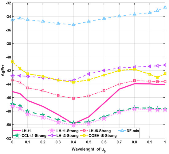
Figure 22.
Aggregated errors (AgErr) as a function of the wavelength in the case of Experiment 13 for the top 7 methods.
Table 12.
Aggregated errors (AgErr) for different wavelength values of the top 7 methods.
7.6. Experiment 14: Sweep for the Wavelength of the β Function
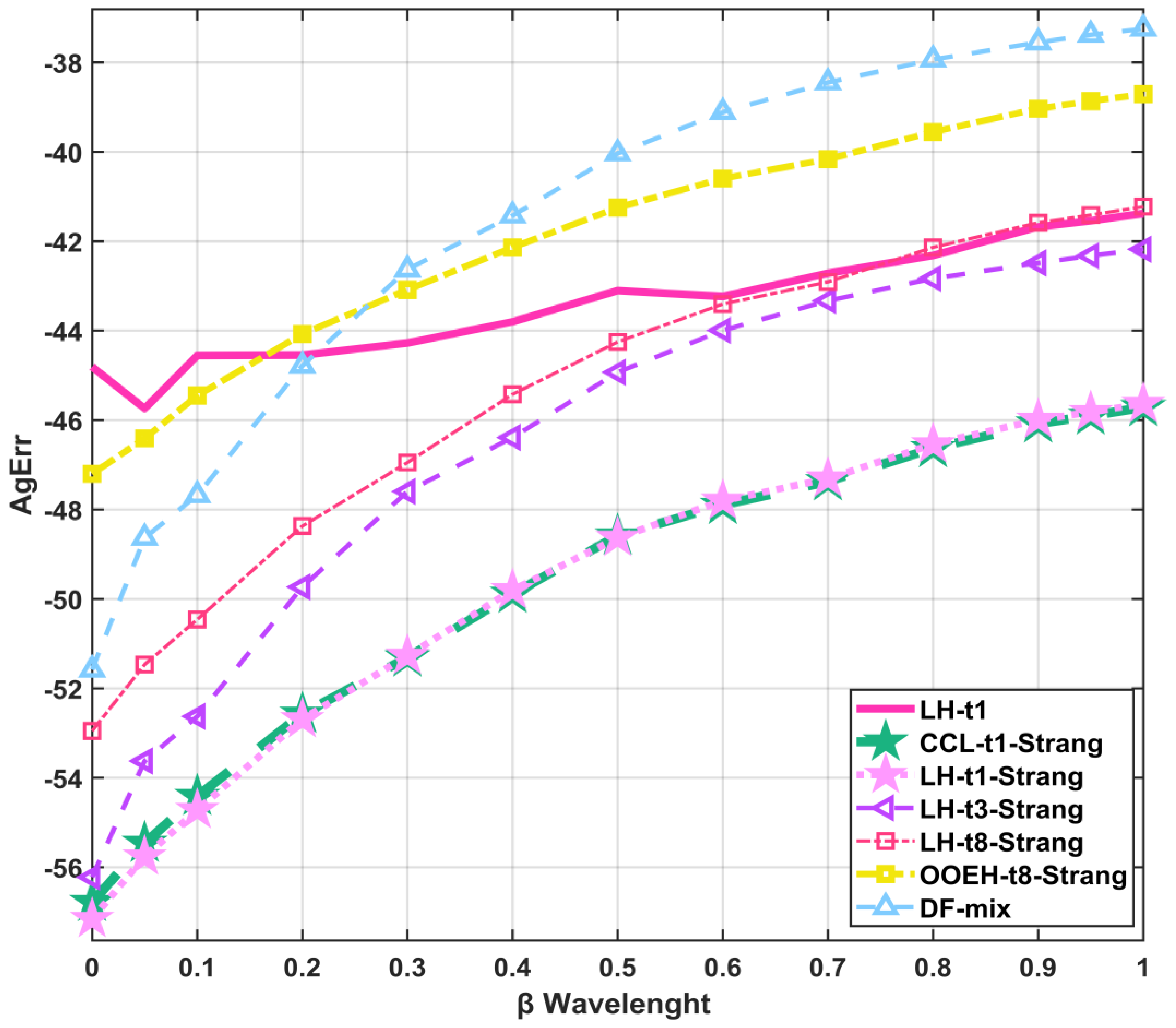
In reality, the reactions can be influenced by the properties of the media, such as temperature, which can depend on space. Therefore, in this subsection, we examine the behavior of the numerical methods under circumstances where the nonlinear coefficient β is a function of space. We construct a long-wave and a short-wave random function, and the function is the weighted average of these different wavelength contributions as follows
where the sweep goes through the parameter values , and the used system size and final time are and . The exponents of C and R are . The initial concentration function is as follows: Figure 23 and Table 13 show the aggregated errors as a function of the wavelength of the β function in the case of Experiment 14 for the top seven methods. The general trend is that the accuracy of the methods is lower when the nonlinear coefficient changes slowly in space. This is particularly true for the DF–mixed method.
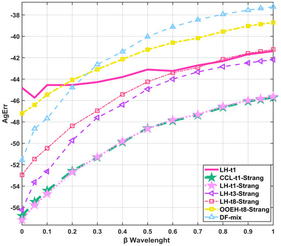
Figure 23.
Aggregated errors (AgErr) as a function of the wavelength of the β function in the case of Experiment 14 for the top 7 methods.
Table 13.
Aggregated errors (AgErr) for different values of the wavelength of the β function for the top 7 methods.
8. Discussion and Conclusions
We performed extensive numerical tests to solve Huxley’s equation. The goal was to explore the performance of some algorithms about which unconditional stability is analytically proven for the linear diffusion equation; thus, excellent stability properties for the nonlinear case were expected. For some, but not all, of the methods, these expectations are fulfilled well.
LH-t1-Strang: According to the numerical tests, the LH with the t1 treatment and Strang-splitting is generally the most efficient and reliable among the examined methods. It provides relatively accurate results quite quickly for all the examined sets of parameters, and no signs of instability are detected, even for extremely stiff systems of strong nonlinearity. Hence, non-strict time step size restrictions are necessary only to reach the desired accuracy, but not for stability considerations.
LH-t1: This combination is usually slightly less accurate than LH-t1 with Strang-splitting. It can be recommended when the diffusion part of the problem is much harder to solve than the reaction part, e.g., due to small β or large stiffness.
LH-t3-Strang: This combination can also give very accurate results, and sometimes it is the most efficient. However, in some cases, for example, if the simulated time interval is long, it is not so reliable.
LH-t8-Strang: Usually slightly less accurate and efficient than the LH-t1-Strang and LH-t3-Strang combinations. If, however, the geometry of the physical system is complicated such that the construction of a bipartite mesh is hardly feasible, the hopscotch-type methods are contraindicated.
OOEH-t8-Strang: The original odd–even hopscotch method can be proposed only for an equidistant mesh with a constant diffusion parameter. In these cases, this method is simpler to code than the LH scheme, and its accuracy is roughly the same.
CCL-t1-Strang: This combination is the opposite of the OOEH method from the point of view that it has a relative disadvantage in the case of a physically homogeneous system with an equidistant mesh. It is relatively slow but reliable for stiff problems. It should be used only if the geometry is complicated and the odd–even division of the cells faces difficulties.
DF–mixed: This combination is much faster and may be beneficially used for complicated geometries. Its accuracy strongly fluctuates; thus, it should be combined with an error estimator.
CrN: In the studied cases where the geometry is simple and the mesh is rectangular, the Crank–Nicolson method with operator-splitting has no advantage against the LH method. Its execution time strongly increases with the system size, so we advise using it only when the number of nodes is small. However, in that case, the CrN method without operator-splitting, i.e., with standard Newton iterations, would be more accurate.
RK4: RK4 should be used if extreme accuracy is required; hence, the above-mentioned low-order methods are not favorable.
AB2: The performance of AB2 is quite similar to the RK4 method due to its similar conditional stability. It is a bit less accurate, but it is faster and requires less memory.
In the near future, we plan to compare the performance of our explicit methods with the following:
- (a)
- Implicit methods (such as Crank–Nicolson) without operator-splitting;
- (b)
- Semi-explicit, semi-implicit, and implicit–explicit schemes;
- (c)
- Runge–Kutta–Chebyshev methods, which are explicit but have improved stability.
Our most important goal is, however, to extend these ideas to more complicated nonlinear diffusion–reaction PDEs (such as the FitzHugh–Nagumo equation) and systems of PDEs.
Supplementary Materials
The following supporting information can be downloaded at: https://www.mdpi.com/article/10.3390/math13020207/s1, Figure S1: Maximum errors as a function of the time step size for different operator-splitting treatments in the case of Experiment 2; Figure S2: Maximum errors as a function of the time step size for different operator-splitting treatments with Strang-splitting in the case of Experiment 2; Figure S3: Maximum errors as a function of time step size for the remaining methods in the case of Experiment 2; Figure S4: Maximum errors as a function of the time step size for different operator-splitting treatments with Strang-splitting in the case of Experiment 3; Figure S5. Maximum errors as a function of the time step size for different operator-splitting treatments with Strang-splitting in the case of Experiment 4; Figure S6. Maximum errors as a function of time step size for the remaining methods in the case of Experiment 4; Figure S7. Maximum errors as a function of time step size for different operator-splitting treatments with Strang-splitting in the case of Experiment 5; Figure S8. Maximum errors as a function of the time step size for the remaining methods in the case of Experiment 5; Figure S9. Maximum errors as a function of the time step size in the case of Experiment 12 for the top 7 methods; Figure S10. Maximum errors as a function of the time step size in the case of Experiment 13 for the top 7 methods for w = 1; Table S1. The Aggregated error (AgErr) values for different treatment of the methods in case of Experiment 6; Table S2. The Aggregated error (AgErr) values for different treatment of the methods in case of Experiment 7; Table S3. The Aggregated errors (AgErr) for different treatments of the methods in case of Experiment 8.
Author Contributions
Conceptualization, methodology, supervision, project administration, and resources, E.K.; software, validation, and investigation, H.K.; writing—original draft preparation, H.K., I.O. and E.K.; writing—review and editing, E.K., I.O. and H.K.; visualization, H.K. and I.O. All authors have read and agreed to the published version of the manuscript.
Funding
This research was funded by the EKÖP-24-4-I, supported by the University Research Scholarship Program of the Ministry for Culture and Innovation from the source of the National Research, Development, and Innovation Fund.
Data Availability Statement
The data are available from the authors on reasonable request.
Conflicts of Interest
The authors declare no conflicts of interest.
References
- Bradshaw-Hajek, B. Reaction-Diffusion Equations for Population Genetics. Ph.D. Thesis, University of Wollongong, Wollongong, NSW, Australia, 2004. [Google Scholar]
- Mohan, M.T.; Khan, A. On the generalized Burgers-Huxley equation: Existence, uniqueness, regularity, global attractors and numerical studies. Discret. Contin. Dyn. Syst. B 2021, 26, 3943–3988. [Google Scholar] [CrossRef]
- Agbavon, K.M.; Appadu, A.R. Construction and analysis of some nonstandard finite difference methods for the FitzHugh–Nagumo equation. Numer. Methods Partial Differ. Equ. 2020, 36, 1145–1169. [Google Scholar] [CrossRef]
- Wang, X. Nerve propagation and wall in liquid crystals. Phys. Lett. A 1985, 112, 402–406. [Google Scholar] [CrossRef]
- Sharma, S.; Prabhakar, N. Numerical Simulation of Generalized FitzHugh-Nagumo Equation by Shifted Chebyshev Spectral Collocation Method. IAENG Int. J. Appl. Math. 2024, 54, 1371–1382. [Google Scholar]
- Lukonde, J.; Kasumo, C. On numerical and analytical solutions of the generalized Burgers-Fisher equation. J. Innov. Appl. Math. Comput. Sci. 2023, 3, 121–141. [Google Scholar]
- Patel, Y.F.; Dhodiya, J.M. Efficient algorithm to study the class of Burger’s Fisher equation. Int. J. Appl. Nonlinear Sci. 2022, 3, 242–266. [Google Scholar] [CrossRef]
- Dhumal, M.; Sontakke, B. Solving Time-Fractional Fitzhugh–Nagumo Equation using Homotopy Perturbation Method. Indian J. Sci. Technol. 2024, 17, 1272–1282. [Google Scholar] [CrossRef]
- Shi, J.; Yang, X.; Liu, X. A novel fractional physics-informed neural networks method for solving the time-fractional Huxley equation. Neural Comput. Appl. 2024, 36, 19097–19119. [Google Scholar] [CrossRef]
- Bai, Y.; Chaolu, T.; Bilige, S. Solving Huxley equation using an improved PINN method. Nonlinear Dyn. 2021, 105, 3439–3450. [Google Scholar] [CrossRef]
- Loyinmi, A.C.; Sanyaolu, M.D.; Gbodogbe, S. Exploring the Efficacy of the Weighted Average Method for Solving Nonlinear Partial Differential Equations: A Study on the Burger-Fisher Equation. Educ. J. Sci. Math. Technol. 2025, 12, 60–79. [Google Scholar] [CrossRef]
- Köroğlu, C.; Aydin, A. Exact and nonstandard finite difference schemes for the Burgers equation B(2,2). Turk. J. Math. 2021, 45, 647–660. [Google Scholar] [CrossRef]
- Jaglan, J.; Maurya, V.; Singh, A.; Yadav, V.S.; Rajpoot, M.K. Acoustic and soliton propagation using fully-discrete energy preserving partially implicit scheme in homogeneous and heterogeneous mediums. Comput. Math. Appl. 2024, 174, 379–396. [Google Scholar] [CrossRef]
- March, N.G.; Carr, E.J.; Turner, I.W. Numerical Investigation into Coarse-Scale Models of Diffusion in Complex Heterogeneous Media. Transp. Porous Media 2021, 139, 467–489. [Google Scholar] [CrossRef]
- Kondratenko, P.S.; Matveev, A.L.; Vasiliev, A.D. Numerical implementation of the asymptotic theory for classical diffusion in heterogeneous media. Eur. Phys. J. B 2021, 94, 50. [Google Scholar] [CrossRef]
- Jejeniwa, O.A.; Gidey, H.H.; Appadu, A.R. Numerical Modeling of Pollutant Transport: Results and Optimal Parameters. Symmetry 2022, 14, 2616. [Google Scholar] [CrossRef]
- Kumar, S.; Ramcharan, B.; Yadav, V.S.; Singh, A.; Rajpoot, M.K. Exploring Acoustic and Sound Wave Propagation Simulations: A Novel Time Advancement Method for Homogeneous and Heterogeneous Media. Adv. Appl. Math. Mech. 2024, 17, 315–349. [Google Scholar] [CrossRef]
- Beuken, L.; Cheffert, O.; Tutueva, A.; Butusov, D.; Legat, V. Numerical Stability and Performance of Semi-Explicit and Semi-Implicit Predictor–Corrector Methods. Mathematics 2022, 10, 2015. [Google Scholar] [CrossRef]
- Ketcheson, D.I. Highly Efficient Strong Stability-Preserving Runge–Kutta Methods with Low-Storage Implementations. SIAM J. Sci. Comput. 2008, 30, 2113–2136. [Google Scholar] [CrossRef]
- Qin, X.; Jiang, Z.; Yan, C. Strong Stability Preserving Two-Derivative Two-Step Runge-Kutta Methods. Mathematics 2024, 12, 2465. [Google Scholar] [CrossRef]
- Anjuman; Leung, A.Y.T.; Das, S. Two-Dimensional Time-Fractional Nonlinear Drift Reaction–Diffusion Equation Arising in Electrical Field. Fractal Fract. 2024, 8, 456. [Google Scholar] [CrossRef]
- Bansal, S.; Natesan, S. A novel higher-order efficient computational method for pricing European and Asian options. Numer. Algorithms 2024. [Google Scholar] [CrossRef]
- Rieth, Á.; Kovács, R.; Fülöp, T. Implicit numerical schemes for generalized heat conduction equations. Int. J. Heat Mass Transf. 2018, 126, 1177–1182. [Google Scholar] [CrossRef]
- Britz, D.; Baronas, R.; Gaidamauskaitė, E.; Ivanauskas, F. Further comparisons of finite difference schemes for computational modelling of biosensors. Nonlinear Anal. Model. Control 2009, 14, 419–433. [Google Scholar] [CrossRef]
- Rufai, M.A.; Kosti, A.A.; Anastassi, Z.A.; Carpentieri, B. A New Two-Step Hybrid Block Method for the FitzHugh–Nagumo Model Equation. Mathematics 2024, 12, 51. [Google Scholar] [CrossRef]
- Chou, C.S.; Zhang, Y.T.; Zhao, R.; Nie, Q. Numerical methods for stiff reaction-diffusion systems. Discret. Contin. Dyn. Syst.-Ser. B 2007, 7, 515–525. [Google Scholar] [CrossRef]
- Manaa, S.; Sabawi, M. Numerical Solution and Stability Analysis of Huxley Equation. AL-Rafidain J. Comput. Sci. Math. 2005, 2, 85–97. [Google Scholar] [CrossRef]
- Macías-Díaz, J.E. On an exact numerical simulation of solitary-wave solutions of the Burgers–Huxley equation through Cardano’s method. BIT Numer. Math. 2014, 54, 763–776. [Google Scholar] [CrossRef]
- Agbavon, K.M.; Appadu, A.R.; Khumalo, M. On the numerical solution of Fisher’s equation with coefficient of diffusion term much smaller than coefficient of reaction term. Adv. Differ. Equ. 2019, 2019, 146. [Google Scholar] [CrossRef]
- Appadu, A.R.; Inan, B.; Tijani, Y.O. Comparative study of some numerical methods for the Burgers-Huxley equation. Symmetry 2019, 11, 1333. [Google Scholar] [CrossRef]
- Songolo, M.E. A Positivity-Preserving Nonstandard Finite Difference Scheme for Parabolic System with Cross-Diffusion Equations and Nonlocal Initial Conditions. Am. Sci. Res. J. Eng. Technol. Sci. 2016, 18, 252–258. [Google Scholar]
- Chapwanya, M.; Lubuma, J.M.S.; Mickens, R.E. Positivity-preserving nonstandard finite difference schemes for cross-diffusion equations in biosciences. Comput. Math. Appl. 2014, 68, 1071–1082. [Google Scholar] [CrossRef]
- Liang, Z.; Yan, Y.; Cai, G. A Dufort-Frankel Difference Scheme for Two-Dimensional Sine-Gordon Equation. Discret. Dyn. Nat. Soc. 2014, 2014, 784387. [Google Scholar] [CrossRef]
- Gasparin, S.; Berger, J.; Dutykh, D.; Mendes, N. Stable explicit schemes for simulation of nonlinear moisture transfer in porous materials. J. Build. Perform. Simul. 2018, 11, 129–144. [Google Scholar] [CrossRef]
- Harley, C. Hopscotch method: The numerical solution of the Frank-Kamenetskii partial differential equation. Appl. Math. Comput. 2010, 217, 4065–4075. [Google Scholar] [CrossRef]
- Nagy, Á.; Saleh, M.; Omle, I.; Kareem, H.; Kovács, E. New stable, explicit, shifted-hopscotch algorithms for the heat equation. Math. Comput. Appl. 2021, 26, 61. [Google Scholar] [CrossRef]
- Kovács, E.; Nagy, Á. A new stable; explicit, and generic third-order method for simulating conductive heat transfer. Numer. Methods Partial Differ. Equ. 2023, 39, 1504–1528. [Google Scholar] [CrossRef]
- Hirsch, C. Numerical Computation of Internal and External Flows, Volume 1: Fundamentals of Numerical Discretization; Wiley: Hoboken, NJ, USA, 1988. [Google Scholar]
- Gourlay, A.R.; McGuire, G.R. General Hopscotch Algorithm for the Numerical Solution of Partial Differential Equations. IMA J. Appl. Math. 1971, 7, 216–227. [Google Scholar] [CrossRef]
- Nagy, Á.; Omle, I.; Kareem, H.; Kovács, E.; Barna, I.F.; Bognar, G. Stable, Explicit, Leapfrog-Hopscotch Algorithms for the Diffusion Equation. Computation 2021, 9, 92. [Google Scholar] [CrossRef]
- Askar, A.H.; Omle, I.; Kovács, E.; Majár, J. Testing Some Different Implementations of Heat Convection and Radiation in the Leapfrog-Hopscotch Algorithm. Algorithms 2022, 15, 400. [Google Scholar] [CrossRef]
- Chapra, S.C.; Canale, R.P. Numerical Methods for Engineers, 7th ed.; McGraw-Hill Science/Engineering/Math: New York, NY, USA, 2015. [Google Scholar]
- Linear Multistep Method. Wikipedia. 23 September 2024. Available online: https://en.wikipedia.org/w/index.php?title=Linear_multistep_method&oldid=1247156850 (accessed on 1 January 2025).


Disclaimer/Publisher’s Note: The statements, opinions and data contained in all publications are solely those of the individual author(s) and contributor(s) and not of MDPI and/or the editor(s). MDPI and/or the editor(s) disclaim responsibility for any injury to people or property resulting from any ideas, methods, instructions or products referred to in the content. |
© 2025 by the authors. Licensee MDPI, Basel, Switzerland. This article is an open access article distributed under the terms and conditions of the Creative Commons Attribution (CC BY) license (https://creativecommons.org/licenses/by/4.0/).