Smoothing Estimation of Parameters in Censored Quantile Linear Regression Model

Abstract

In this paper, we propose a smoothing estimation method for censored quantile regression models. The method associates the convolutional smoothing estimation with the loss function, which is quadratically derivable and globally convex by using a non-negative kernel function. Thus, the parameters of the regression model can be computed by using the gradient-based iterative algorithm. We demonstrate the convergence speed and asymptotic properties of the smoothing estimation for large samples in high dimensions. Numerical simulations show that the smoothing estimation method for censored quantile regression models improves the estimation accuracy, computational speed, and robustness over the classical parameter estimation method. The simulation results also show that the parametric methods perform better than the KM method in estimating the distribution function of the censored variables. Even if there is an error setting in the distribution estimation, the smoothing estimation does not fluctuate too much.

1. Introduction

Since the regression quantile has similar robustness as the sample quantile, the quantile regression model can well characterize the conditional distribution of the response variable y when the independent variable $\mathit{x}$ is given, thus characterizing the link between the two [1]. Response variable $y\in \mathbb{R}$ and p-dimensional covariates $\mathit{x}={(x_1,...,x_p)}^T$ are given, and $F_{y|\mathit{x}}(·)$ is the conditional distribution function of y concerning $\mathit{x}$. The classical quantile regression model can be expressed as

$$\begin{array}{c}\hfill F_{y|\mathit{x}}^{-1}\left(\tau \right)={\left[\mathit{\beta }\left(\tau \right)\right]}^T\mathit{x},\end{array}$$

(1)

where $\mathit{\beta }=\mathit{\beta }\left(\tau \right)={({\beta }_1\left(\tau \right),...,{\beta }_p\left(\tau \right))}^T\in {\mathbb{R}}^p$ is the regression coefficient. Koenker, R. et al. [2,3] provided a detailed discussion of quantile regression modeling in terms of methodology, theory, and computation. Because the loss function of quantile regression is not smooth, its computational complexity increases dramatically. Considering that the loss function is not derivable, Horowitz [4] used the smooth function to approximate the indicator function, in order to smooth the objective function. This method has also been applied to deal with other quantile regression-related problems, in which de Castro, L. et al. [5] used a smooth moment estimating equation to estimate the parameter in quantile regression; Chen et al. [6] used a smoothing method to study the quantile regression model with constraints; Galvao, A.F. and Kato, K. [7] studied the smoothing estimation of fixed effects in quantile regression models for panel data; Whang [8] discussed the empirical likelihood estimation of quantile regression models by using a smoothing approach. Although the above literature has solved the problem that the objective function is not derivable, it cannot guarantee the concavity of the objective function. Thus, there is no guarantee that the result is a global optimal solution. Recently, Fernandes et al. [9] proposed a convolutional smoothing method for estimating fixed dimensional parameters of the quantile regression model, based on which the loss function is quadratically derivable and convex, and the method outperforms the original smoothing estimation in terms of estimation accuracy. Under the complete observation data, He [10] used the convolutional smoothing method to estimate the parameters of the high-dimensional quantile regression model, and the loss function after smoothing is a quadratically derivable and convex function. When solving the minimum point of the smoothed objective function numerically, the gradient descent algorithm [10] is used to replace the quantile regression with the least squares estimation, which effectively shortens the computation time and improves the estimation accuracy.

In empirical studies, it is frequently observed that variables of interest are subject to censoring. For instance, in the study [11] on the survival times of AIDS patients, it was found that 43% of the data were right-censored. For parameter estimation in quantile regression models for right-censored data, we refer to Ying, Z. et al. [12], Honoré, B. et al. [13], Portnoy, S. [14], Peng, L. [15], and Yuan, X. et al. [16]. Parameter estimation in quantile regression models for censored data [17,18,19] has been extensively studied, including right-censored data. In the quantile regression for right-censored data, the problem of non-smooth loss functions still exists, and it has already been studied [20,21,22,23]. For the right-censored quantile regression model with fixed dimensional parameters, Peng, L. and Huang, Y. [20], Xu, G. et al. [21], Cai, Z. and Sit, T. [22], Kim, K.H. [23] considered the smoothing estimation methods, respectively. For the high-dimensional large-sample case of the censored quantile regression model, Wu, Y. et al. [24], He, X. et al. [25], and Fei, Z. et al. [26] used a similar method to Fernandes et al. [9] to smooth the estimating equations, which improved the estimation accuracy over classical parameter estimation methods. However, these smoothing estimation methods for high-dimensional censored quantile regression need to grid the quantiles as $0={\tau }_1<\cdots <{\tau }_j<{\tau }_{j+1}\cdots <{\tau }_k=1$, to ensure that the approximation error of the estimation equation will not be too large. Furthermore, we need to use the estimates of $\mathit{\beta }\left({\tau }_1\right),\cdots ,\mathit{\beta }\left({\tau }_j\right)$ before estimating $\mathit{\beta }\left({\tau }_{j+1}\right)$, and the estimation accuracy depends on the number of segmentation points, which also increases the computational complexity.

Considering the censored data, this paper extends the convolutional smoothing method [10] to the high-dimensional censored quantile regression model and proposes the coefficient estimation of the censored quantile regression model based on the convolutional smoothing method. Under certain conditions, the loss function of the smoothed censored quantile regression model is quadratically derivable and globally convex, and the gradient-based iterative algorithm could be used to calculate the regression parameters. In this paper, the bias of the smoothing estimation of the censored quantile regression is characterized under certain conditions, and the speed of convergence, the Bahadur–Kiefer representation, and the Berry–Esseen upper bound of the smoothing estimation of the censored quantile regression are established under high-dimensional and large-sample conditions. Moreover, compared with the classical parameter estimation method, which has different estimation accuracies at different quantile points, the smoothing estimation method basically maintains the same estimation accuracies at each quantile point, and the proposed method greatly saves the computation time under high-dimensional large-sample condition. In summary, the key contributions and significance of this article are as follows: (1) To our knowledge, this article is the first to apply the convolutional smoothing method to high-dimensional censored data regression analysis. Compared with the non differentiability of the objective function in classical censored quantile regression, the objective function in this method is second-order differentiable, which brings great convenience to the establishment of gradient based calculation algorithms and the discussion of theoretical properties. (2) For high-dimensional data scenarios, under certain regularization conditions, this paper also establishes the asymptotic consistency, asymptotic normality, and other theoretical properties of the proposed smooth estimator, ensuring the good properties of statistical inference.

This paper is organized as follows. Section 2 proposes a convolutional smoothing estimation method for high-dimensional censored quantile regression models, and gives the asymptotic properties of the smoothing estimation. In Section 3, numerical simulations of the smoothing estimation and the classical parameter estimation are carried out for the low and high dimensional cases, and the estimation accuracy and computational speed of the smoothing method in the censored quantile regression analysis are discussed. The discussion and conclusion are given in Section 4 and Section 5, and then a detailed proof of the asymptotic property is given in Appendix A.

2. Methods

In this paper, we consider a right-censored quantile regression model; i.e., we assume that the response variable y in the model (1) is right-censored, in which case the observed variables are $z=min(y,c),\delta =\mathbb{I}(y\le c)$, where c is the censored variable. The observations are denoted as $\{(z_i,{\mathit{x}}_i,{\delta }_i),i=1,...,n\}$. Then, the estimation of the parameters in the censored quantile regression model is defined as

$$\begin{array}{c}\hfill \widehat{\mathit{\beta }}\left(\tau \right)\in \underset{\mathit{\beta }\in {\mathbb{R}}^p}{min}Q\left(\mathit{\beta }\right)=\underset{\mathit{\beta }\in {\mathbb{R}}^p}{min}{\displaystyle \frac{1}{n}}\sum _{i=1}^n{\displaystyle \frac{{\delta }_i}{1-\widehat{G}\left(z_i\right)}}{\rho }_{\tau }(z_i-{\mathit{\beta }}^T{\mathit{x}}_i),\end{array}$$

(2)

where ${\rho }_{\tau }\left(u\right)=u\{\tau -\mathbb{I}(u<0)\}$ is the $\tau$ quantile loss function, and $G(·)$ is the distribution function of the censored variable $c_i$, and $\widehat{G}(·)$ is the estimate of $G(·)$.

Convolutional smoothing estimation for high-dimensional quantile regression models has been studied in the literature [10] by He et al. In this paper, we apply the method to censored data. Let $K(·)$ be the kernel function with integral 1, and h be the window width. Denote the following:

$$\begin{array}{c}\hfill K_h\left(u\right)=h^{-1}K(u/h),{\mathcal{K}}_h\left(u\right)=\mathcal{K}(u/h),\mathcal{K}\left(u\right)={\int }_{-\infty }^{u}K\left(\mathit{\upsilon }\right)\mathrm{d}\mathit{\upsilon },u\in \mathbb{R}.\end{array}$$

Then, the objective function for the smoothing estimation of the censored quantile regression can be written as

$$\begin{array}{c}\hfill Q_h\left(\mathit{\beta }\right)={\displaystyle \frac{1}{n}}\sum _{i=1}^n{\displaystyle \frac{{\delta }_i}{1-\widehat{G}\left(z_i\right)}}{\ell }_h(z_i-{\mathit{\beta }}^T\mathit{x}),\end{array}$$

(3)

where ${\ell }_h\left(u\right)=({\rho }_{\tau }\ast K_h)\left(u\right)={\int }_{-\infty }^{+\infty }{\rho }_{\tau }\left(\upsilon \right)K_h(\upsilon -u)\mathrm{d}\upsilon$ and “∗” denotes the convolution operator. The convolutional smoothing estimate (denoted SCQ) of the censored quantile regression model is defined as the point of minimum of $Q_h\left(\mathit{\beta }\right)$, ${\widehat{\mathit{\beta }}}_h$. For any $\mathit{\beta }\in {\mathbb{R}}^p$, write $Q_h^{*}\left(\mathit{\beta }\right)=\mathbb{E}{Q}_h\left(\mathit{\beta }\right)$, with

$$\begin{array}{c}\hfill {\mathit{\beta }}_h^{*}\left(\tau \right)\in {\mathrm{argmin}}_{\mathit{\beta }\in {\mathbb{R}}^p}{Q}_h^{*}\left(\mathit{\beta }\right).\end{array}$$

(4)

For ease of presentation and without ambiguity, ${\mathit{\beta }}^{*}\left(\tau \right)\in {\mathrm{argmin}}_{\mathit{\beta }\in {\mathbb{R}}^p}\mathbb{E}Q\left(\mathit{\beta }\right)$ and ${\mathit{\beta }}_h^{*}\left(\tau \right)$ are abbreviated as ${\mathit{\beta }}^{*}$ and ${\mathit{\beta }}_h^{*}$, respectively.

It is easy to find that the loss function of the (3) is quadratically derivable, and its gradient and Hessian matrix can be expressed, respectively, as follows:

$$\nabla Q_h\left(\mathit{\beta }\right)={\displaystyle \frac{1}{n}}\sum _{i=1}^n{\displaystyle \frac{{\delta }_i}{1-\widehat{G}\left(z_i\right)}}\{{\mathcal{K}}_h({\mathit{\beta }}^T{\mathit{x}}_i-z_i)-\tau \}{\mathit{x}}_{\mathit{i}},$$

(5)

$${\nabla }^2{Q}_h\left(\mathit{\beta }\right)={\displaystyle \frac{1}{n}}\sum _{i=1}^n{\displaystyle \frac{{\delta }_i}{1-\widehat{G}\left(z_i\right)}}{K}_h(z_i-{\mathit{\beta }}^T{\mathit{x}}_i){\mathit{x}}_{\mathit{i}}{\mathit{x}}_{\mathit{i}}^T.$$

As long as the kernel function $K(·)$ is non-negative, for any window width $h>0$, $Q_h\left(\mathit{\beta }\right)$ is a convex function and ${\mathit{\beta }}_h^{*}={\mathit{\beta }}_h^{*}\left(\tau \right)$ satisfies the first-order condition $\nabla Q_h\left({\mathit{\beta }}_h^{*}\right)=0$.

Remark 1. 

When estimating the distribution of the censored variable $c_i$, we can use KM estimation to estimate $\widehat{G}(·)$. If we assume that the form of the distribution $G(·)$ of the censored variable $c_i$ is known, even if there is a mis-specification of the distribution, we find through the subsequent simulation that the estimation of the distribution of the censored variable by the parametric method is better than that of the distribution of the censored variable by using the KM estimation before smoothing the estimation of the regression parameter in most cases; thus, we rewrite the distribution function of the censored variable $c_i$ as follows $\widehat{G}(·)=G(·,{\widehat{\mathit{\theta }}}_n)$. Where the parameter vector ${\mathit{\theta }}_n\in {\mathbb{R}}^p$, ${\widehat{\mathit{\theta }}}_n$ is the maximum likelihood estimate of ${\mathit{\theta }}_n$. The parametric distribution form is used for estimation in both the proof and the hypotheses.

To give theoretical results, we assume that the covariate $\mathit{x}$ has been centered. Given the vectors $\mathit{u},\mathit{\upsilon }\in {\mathbb{R}}^p$, ${\mathit{u}}^T\mathit{\upsilon }$ and $⟨\mathit{u},\mathit{\upsilon }⟩$ both represent their inner product: $a\vee b=max\{a,b\}$, where a and b are constants. The ${∥·∥}_q(1\le q<\infty )$ denotes the ${\ell }_q$-paradigm, i.e., ${∥\mathit{u}∥}_q=({\sum }_{i=1}^p|u_i{{|}^q)}^{1/q}$, and ${∥\mathit{u}∥}_{\infty }={max}_{1\le i\le p}\left|u_i\right|$, where $u_i$ denotes the ith element of the p-dimensional real vector $\mathit{u}$. Given a semi-positive definite matrix $\mathbf{\Sigma }\in {\mathbb{R}}^{p\times p}$, define ${∥\mathit{u}∥}_{\mathbf{\Sigma }}={\parallel {\mathbf{\Sigma }}^{1/2}\mathit{u}\parallel }_2$ for any vector $\mathit{u}\in {\mathbb{R}}^p$. For all real numbers $r\ge 0$, define ${\mathbb{B}}^p\left(r\right)=\{\mathit{\beta }\in {\mathbb{R}}^p{:\parallel \mathit{\beta }\parallel }_2\le r\}$ and ${\mathbb{S}}^{p-1}\left(r\right)=\{\mathit{\beta }\in {\mathbb{R}}^p{:\parallel \mathit{\beta }\parallel }_2=r\}$. For two non-negative sequences ${\left\{a_n\right\}}_{n\ge 1}$ and ${\left\{b_n\right\}}_{n\ge 1}$, $a_n\lesssim b_n$ denotes the existence of a constant $C>0$ independent of n such that $a_n\le C{b}_n$. $a_n\gtrsim b_n$ is equivalent to $b_n\lesssim a_n$. $a_n\asymp b_n$ is equivalent to $a_n\lesssim b_n$ and $b_n\lesssim a_n$ holds simultaneously. The assumptions required for the theorem are as follows.

$\mathit{A}\mathbf{1}$. The non-negative kernel function $K(·)$ satisfies $K\left(u\right)=K(-u)$, with upper bound $\kappa :={sup}_{u\in \mathbb{R}}K\left(u\right)<+\infty$, and ${\kappa }_k:={\int }_{-\infty }^{+\infty }{\left|u\right|}^{k}K\left(u\right)\mathrm{d}u<+\infty$, where $k=1,2$.

$\mathit{A}\mathbf{2}$. The regression error term $\epsilon$ on the conditional density function $f_{\epsilon |\mathit{x}}(·)$ on $\mathit{x}$ satisfies the Lipschtiz condition; i.e., there exists a constant $L>0$ such that $\forall u,\upsilon \in \mathbb{R}$, there is $|f_{\epsilon |\mathit{x}}\left(u\right)-f_{\epsilon |\mathit{x}}\left(\upsilon \right)|\le L|u-\upsilon |$ which holds almost everywhere. There exist real numbers $\underline{f}>0$ such that $f_{\epsilon |\mathit{x}}\left(0\right)\ge \underline{f}$ holds almost everywhere for any $\mathit{x}$.

$\mathit{A}\mathbf{3}$. There exist positive constants $C_1$ and $K_j$ such that

$$\begin{array}{c}\hfill {\displaystyle \frac{\partial G(z;\mathit{\theta })}{\partial {\mathit{\theta }}_j}}\le K_j\left(z\right),E\left\{K_j^2\left(z\right)\right\}\le C_1<\infty .(j=1,...,d)\end{array}$$

(6)

Denote $z_{\left(i\right)}$ as the ith order statistic of $\left\{z_i\right\}$, and ${\delta }_{\left(i\right)}$ as the corresponding indicator function. $z_{\left(i\right)}$ and ${\delta }_{\left(i\right)}$ satisfy

$$\begin{array}{c}\hfill \mathbb{P}({\delta }_{\left(n\right)}=1|z_{\left(n\right)})>0.\end{array}$$

(7)

$\mathit{A}\mathbf{4}$. The covariate $\mathit{x}$ obeys a subexponential distribution—i.e., there exists ${\upsilon }_0>0$ such that for any $\mathit{u}\in {\mathbb{S}}^{p-1}$ and $t\ge 0$, there are $\mathbb{P}\left\{\right|\mathit{u},\mathit{\omega }|\ge {\upsilon }_{0}t\}\le e^{-t}$, where $\mathbf{\Sigma }=\mathbb{E}\left\{\mathit{x}{\mathit{x}}^T\right\}$ is positive definite with $\mathit{\omega }={\mathbf{\Sigma }}^{-1/2}\mathit{x}$.

With $\mathit{\omega }={\mathbf{\Sigma }}^{-1/2}\mathit{x}$ and positive integer k, we define $m_k={sup}_{\mathit{u}\in {\mathbb{S}}^{p-1}}\mathbb{E}{\left|⟨\mathit{u},\mathit{\omega }⟩\right|}^k$. The following theorems can be obtained.

Theorem 1 

(Upper bound on the estimation error). Suppose the condition $\mathit{A}\mathbf{1}$–$\mathit{A}\mathbf{4}$ holds for any real number $t>0$. If h satisfies the constraints ${\underline{f}}^{-1}{m}_3^{1/2}{\mathit{\upsilon }}_0^{*}\sqrt{P_d(p+t)/n}\lesssim h\lesssim \underline{f}{m}_3^{-1/2}$, $P_d={\displaystyle \frac{{\sum }_i{\delta }_i}{n}}$ is the uncensored proportion, then the convolutional smoothing estimate ${\widehat{\mathit{\beta }}}_h$ satisfies the boundary conditions

$$\begin{array}{c}\hfill \mathbb{P}\left\{\parallel {\widehat{\mathit{\beta }}}_h-{\mathit{\beta }}^{*}{\parallel }_{\mathbf{\Sigma }}\le {\displaystyle \frac{R}{\underline{f}}}\left[{\mathit{\upsilon }}_0^{*}\sqrt{{\displaystyle \frac{log\left(log(\frac{1}{h}\vee 1)\right)+p+t}{n}}}+L{\kappa }_2{h}^2\right]\right\}\ge 1-2e^{-t},\end{array}$$

(8)

where ${\upsilon }_0^{*}=C_0{\upsilon }_0$. $C_0$ and R are positive constants.

The upper bounds on the estimation error ${\upsilon }_0^{*}\sqrt{{\displaystyle \frac{log\left(log(\frac{1}{h}\vee 1)\right)+p+t}{n}}}$ and $L{\kappa }_2{h}^2$ can be interpreted as the prediction bias and the speed of convergence. A smaller h leads to smaller deviations after smoothing, but an h that is too small could result in overfitting and slow convergence rates. According to Theorem 1, h satisfies the condition $\sqrt{(p+t)/n}\lesssim h\lesssim 1$. In order to obtain a non-asymptotic Bahadur representation of the smoothing estimation, we tend to replace $\mathit{A}\mathbf{4}$ with $\mathit{A}{\mathbf{4}}^{*}$.

$\mathit{A}{\mathbf{4}}^{*}$. The covariate $\mathit{x}$ obeys a sub-Gaussian distribution—i.e. there exists ${\upsilon }_1>0$ such that for any $\mathit{u}\in {\mathbb{S}}^{p-1}$ and $t\ge 0$, there is a $\mathbb{P}\left\{\right|\mathit{u},\mathit{\omega }|\ge {\upsilon }_{1}t\}\le 2e^{-t^2/2}$, where $\mathbf{\Sigma }=\mathbb{E}\left\{\mathit{x}{\mathit{x}}^T\right\}$ is positive definite with $\mathit{\omega }={\mathbf{\Sigma }}^{-1/2}\mathit{x}$.

Theorem 2 

(non-asymptotic Bahadur representation). Assuming conditions $\mathit{A}\mathbf{1}$–$\mathit{A}\mathbf{3}$ and $\mathit{A}{\mathbf{4}}^{*}$ hold, ${sup}_{u\in \mathbb{R}}{f}_{\epsilon |\mathit{x}}\left(u\right)\le \overline{f}$ holds almost everywhere. For any real number $t>0$, h satisfies the constraint ${\underline{f}}^{-1}{m}_3^{1/2}{\upsilon }_1^{*}\sqrt{P_d(p+t)/n}\lesssim h\lesssim \underline{f}{m}_3^{-1/2}$. Let ${\mathit{J}}_h={\nabla }^2{Q}_h\left({\mathit{\beta }}^{*}\right)=\mathbb{E}\left\{{\left[{\displaystyle \frac{\delta }{1-G\left(z\right)}}\right]}^2{K}_h\left(\epsilon \right)\mathit{x}{\mathit{x}}^T\right\}$; then,

$$\begin{array}{cc}\hfill \mathbb{P}\{\parallel {\mathit{J}}_h({\widehat{\mathit{\beta }}}_h-{\mathit{\beta }}^{*})-{\displaystyle \frac{1}{n}}\sum _{i=1}^n\{\tau -{\mathcal{K}}_h(-{\epsilon }_i)\}{\mathit{x}}_{\mathit{i}}{\parallel }_{\mathbf{\Sigma }}\le & R\left({\displaystyle \frac{p+t}{n{h}^{1/2}}}+h^{3/2}·\sqrt{{\displaystyle \frac{p+t}{n}}}+h^4\right)\}\hfill \\ \hfill \ge & 1-3e^{-t},\hfill \end{array}$$

(9)

where the real number $R>0$ is a constant independent of p and n.

Theorem 2 allows for establishing the limiting distribution of the estimators. Based on the non-asymptotic representation in Theorem 2, we establish the Berry–Esseen upper bound for smoothing estimators.

Theorem 3 

(Berry–Esseen upper bound). Assuming that the conditions $\mathit{A}\mathbf{1}$–$\mathit{A}\mathbf{3}$ and $\mathit{A}{\mathbf{4}}^{*}$ hold, ${sup}_{u\in \mathbb{R}}{f}_{\epsilon |\mathit{x}}\left(u\right)\le \overline{f}$ holds almost everywhere, and h satisfies the condition that for any real number $t>0$, there exists $\sqrt{{\displaystyle \frac{p+t}{n}}}\lesssim h\lesssim 1$. Then,

$$\begin{array}{c}\hfill {\mathrm{\Lambda }}_{n,p}\left(h\right):=\underset{x\in \mathbb{R},\mathit{a}\in {\mathbb{R}}^p}{sup}\left|\mathbb{P}(n^{1/2}{\sigma }_h^{-1}⟨\mathit{a},{\widehat{\mathit{\beta }}}_h-{\mathit{\beta }}^{*}⟩\le x)-\mathrm{\Phi }\left(x\right)\right|\lesssim {\displaystyle \frac{p+logn}{{\left(nh\right)}^{1/2}}}+n^{1/2}{h}^2,\end{array}$$

(10)

where ${\sigma }_h^2={\sigma }_h^2\left(\mathit{a}\right)={\mathit{a}}^T{\mathit{J}}_h^{-1}\mathbb{E}\left[{\left({\displaystyle \frac{\delta }{1-G\left(z\right)}}\right)}^2{\{{\mathcal{K}}_h(-\epsilon )-\tau \}}^2\mathit{x}{\mathit{x}}^T\right]{\mathit{J}}_h^{-1}\mathit{a}$, $\mathrm{\Phi }(·)$ denotes the standard normal distribution function.

Further, if $f_{\epsilon |\mathit{x}}(·)$ is quadratically continuously derivable and satisfies $|f_{\epsilon |\mathit{x}}^{″}\left(u\right)-f_{\epsilon |\mathit{x}}^{″}\left(\upsilon \right)|\le l_2\left(\mathit{x}\right)|u-\upsilon |$ for any real number $u,\upsilon \in \mathbb{R}$, where the function $l_2:{\mathbb{R}}^p\to {\mathbb{R}}^{+}$ satisfies $\mathbb{E}\left\{l_2^2\left(\mathit{x}\right)\right\}\le C$ for some positive constant C, then

$$\begin{array}{cc}\hfill \underset{x\in \mathbb{R},\mathit{a}\in {\mathbb{R}}^p}{sup}\left|\mathbb{P}\right(n^{1/2}{\sigma }_h^{-1}⟨\mathit{a},{\widehat{\mathit{\beta }}}_h-{\mathit{\beta }}^{*}& +0.5{\kappa }_2{h}^2{\mathit{J}}_h^{-1}\mathbb{E}\left\{f_{\epsilon |\mathit{x}}^{\prime }\left(0\right){\mathit{x}}_{\mathit{i}}\right\}⟩)-\mathrm{\Phi }\left(x\right)|\hfill \end{array}$$

$$\begin{array}{c}\hfill \lesssim {\displaystyle \frac{p+logn}{{\left(nh\right)}^{1/2}}}+{(p+logn)}^{1/2}{h}^{3/2}+n^{1/2}{h}^4.\end{array}$$

(11)

Theorem 3 proves that when h is chosen in the appropriate range and $n,p\to \infty$, the linear combination of ${\widehat{\mathit{\beta }}}_h$ is estimated to be asymptotically normal. According to Theorem 3, the optimal $h={\{(p+logn)/n\}}^{2/5}$ in the sense that minimizes the right hand of $\left(10\right)$, and the error is approximated as ${(p+logn)}^{4/5}{n}^{-3/10}$. If $p^8/n^3\to 0$, for any given vector $\mathit{a}\in {\mathbb{R}}^p$, $n^{1/2}⟨\mathit{a},{\widehat{\mathit{\beta }}}_h-{\mathit{\beta }}^{*}⟩$ is asymptotically normal.

Remark 2. 

The assumptions $\mathit{A}\mathbf{1}$, $\mathit{A}\mathbf{2}$, $\mathit{A}\mathbf{4}$ and $\mathit{A}{\mathbf{4}}^{*}$ are commonly used in convolutional smoothing estimation of high-dimensional quantile regression models in fully observed data [10]. Condition $\mathit{A}\mathbf{3}$ refers to the assumptions concerning the distribution of the censoring variable c. Note that $\mathbb{P}({\delta }_{\left(n\right)}=1|z_{\left(n\right)})=\mathbb{P}(z_{\left(n\right)}\le c|z_{\left(n\right)})={\int }_{z_{\left(n\right)}}^{+\infty }\mathrm{d}G\left(s\right)=1-G\left(z_{\left(n\right)}\right)$, assuming that $\mathbb{P}({\delta }_{\left(n\right)}=1|z_{\left(n\right)})>0$ is equivalent to $G\left(z_{\left(n\right)}\right)<1$—i.e., the probability that the largest observation $z_{\left(n\right)}$ equals to the true variable of interest is not zero.This is a commonly used condition in statistical inference for censored data [27,28], and this condition can avoid the situation where a large number of observations are censored data. Assuming that $\left(6\right)$ provides a local smoothing condition for $G(·)$ in the neighborhood θ, the validity of this assumption could be verified intuitively for many commonly used distribution functions $G(·)$.

3. Numerical Simulation

In this section, the smoothing estimation and classical parameter estimation of the quantile regression model for censored data are numerically simulated, and two cases of low and high dimensionality are considered. Estimation of (2), as proposed in the literature [17], was chosen as the classical parameter estimation of the censored quantile regression model. Notice that the objective function of the classical parameter estimation for censored quantile regression model can be rewritten as $Q\left(\mathit{\beta }\right)={\sum }_{i=1}^n{\rho }_{\tau }\left[{\displaystyle \frac{{\delta }_i}{1-G\left(z_i\right)}}(z_i-{\mathit{\beta }}^{\mathit{T}}\mathit{x})\right]$. Therefore, when calculating the regression parameters, the censoring problem is transformed into a non-censoring problem, and the objective function of the smoothing estimation for censored quantile regression is rewritten as $Q_h\left(\mathit{\beta }\right)={\sum }_{i=1}^n{\ell }_h\left[{\displaystyle \frac{{\delta }_i}{1-G\left(z_i\right)}}(z_i-{\mathit{\beta }}^{\mathit{T}}\mathit{x})\right]$. The Gaussian kernel and window width $h={\{(p+logn)/n\}}^{2/5}$ are taken as the kernel function and window width, respectively, for the smoothing estimation of the censored quantile regression.

3.1. Model Setting and Evaluation Indicators

In the simulation, the covariates ${\mathit{x}}_i={(x_{i1},...,x_{ip})}^T\in {\mathbb{R}}^p$ are generated from different distributions to simulate different types of variables commonly found in real data. The error term ${\epsilon }_i$ is generated by three different distributions, specifically, by drawing independent identically distributed random numbers ${\tilde{\epsilon }}_i$ with capacity n, and letting ${\epsilon }_i={\tilde{\epsilon }}_i-F_{{\tilde{\epsilon }}_i}^{-1}\left(\tau \right)$, where ${\tilde{\epsilon }}_i$ obeys the distributions: $\left(i\right)t\left(4\right)$; $\left(ii\right){\chi }^2\left(1\right)$; $\left(iii\right)Laplace(0,1)$. Let the regression coefficient $\mathit{\beta }={(1,...,1)}^T\in {\mathbb{R}}^p$, given the quantile $\tau \in (0,1)$; then, the response variable $y_i$ is modeled by

$$\begin{array}{c}\hfill y_i={\beta }_1{x}_{i1}+{\beta }_2{x}_{i2}+...+{\beta }_p{x}_{ip}+{\epsilon }_i.\end{array}$$

For both low- and high-dimensional models, the right censoring variable is set as $c_i\sim const+E\left(pa\right)$, where $const,pa$ are unknown parameters, which can take different values to make the censoring ratio of the response variable $y_i$ up to the set 15%, 30%, or 45%. In the actual simulation, in order to obtain the value of $G\left(z_i\right)$, the parameters $const,pa$ are estimated by using maximum likelihood estimation in the simulations of Section 3.2 and Section 3.3. In Section 3.4, we discuss the smoothing estimation under the misspecification for the distribution of censored variables. KM estimation is also taken into consideration. Let the number of simulation repetitions be K, and for the parameter estimates $\widehat{\mathit{\beta }}$ in the kth simulation, write

$$\begin{array}{c}\hfill S{E}_k={\displaystyle \frac{1}{p}}{\parallel \widehat{\mathit{\beta }}-\mathit{\beta }\parallel }_2^2,\end{array}$$

Then, we can use

$$\begin{array}{c}\hfill DMSE={\displaystyle \frac{1}{K}}\sum _{k=1}^{K}S{E}_k,\end{array}$$

to evaluate the performance of classical parameter estimation for censored quantile regression models (CQ) and smoothing estimation methods (SCQ). In the actual simulation, we set $K=500$.

3.2. Low-Dimensional Performance of Regression Smoothing Estimates for Censored Quantiles

In the low-dimensional numerical study of smoothing estimation, the number of covariates is set to be $p=5$ and sample sizes are 100, 200, and 500. In order to assess the performance of smoothing method in the low-dimensional case, the generation of covariates is categorized into three cases.

• Case 1: The p-dimensional covariates are generated from multivariate uniform distribution on ${[10,20]}^p$, and the covariance matrix is a unit matrix;
• Case 2: The p-dimensional covariate is generated from multivariate uniform distribution on ${[10,20]}^p$, where $\mathbf{\Sigma }={(0.5^{|j-k|})}_{1\le j,k\le p}$ is the covariance matrix;
• Case 3: The p-dimensional covariates consist of a mixture of distributions, where the first two dimensional covariates are generated by a multivariate uniform distribution on ${[10,20]}^2$, with a covariance matrix of ${\mathbf{\Sigma }}_1={(0.5^{|j-k|})}_{1\le j,k\le 2}$. The covariates in the posterior three dimensions are generated from $N(\mathit{\mu },{\mathbf{\Sigma }}_2)$ with mean $\mathit{\mu }=(11,12,13)$ and covariance matrix ${\mathbf{\Sigma }}_2={\left({\sigma }_{jk}\right)}_{1\le j,k\le p}$, where

  $${\sigma }_{jk}=\left\{\begin{array}{cc}\hfill 0.2^{|j-k|}& ,1\le j\ne k\le p,\hfill \\ \hfill 3& ,1\le j=k\le p.\hfill \end{array}\right.$$

Table 1, Table 2 and Table 3 show the simulation results when the covariates are generated according to the three scenarios, where CP denotes the censoring ratio of the response variable, n is the sample size, and columns 3–12 show the results of CQ and SCQ at different quantiles. From the estimation results, when the regression errors are generated by symmetric distributions, i.e., t and Laplace distributions, SCQ has higher accuracy than CQ, especially at the lower and higher quantiles. When the regression error term is generated by the ${\chi }^2$ distribution, the estimation accuracy of CQ decreases as $\tau$ increases from a global perspective, and the estimation accuracy of SCQ is much better than that of CQ at the higher quantiles, although CQ is better than SCQ at the lower quantiles. This may be because the density function of the ${\chi }^2$ distribution is biased and the observations are excessively clustered in the lower quantiles, so that CQ decreases in estimation accuracy as the number of quantiles increases, while SCQ maintains better estimation accuracy. It can be seen from Table 1, Table 2 and Table 3 that SCQ is more stable than CQ, regardless of whether the error terms follow symmetric or asymmetric distribution. Specifically, the estimation accuracy of SCQ is almost the same in all quantiles, while that of CQ fluctuates with the change of $\tau$, especially in the case of the asymmetric distribution of the error terms. Overall, the estimation accuracy of CQ depends greatly on the value of $\tau$, the size of the censoring ratio, and the distribution of the error term, while the estimation effect of SCQ is minimally affected by these factors and shows good robustness.

Table 1. The DMSE of CQ and SCQ estimators for the low-dimensional model with covariate X generated from Case 1, where the values in columns 3–12 are DMSE ×${10}^4$.

$\mathit{CP}\%$	$\mathit{n}$	$\mathit{\tau }=0.1$		$\mathit{\tau }=0.3$		$\mathit{\tau }=0.5$		$\mathit{\tau }=0.7$		$\mathit{\tau }=0.9$
		CQ	SCQ	CQ	SCQ	CQ	SCQ	CQ	SCQ	CQ	SCQ
${\tilde{\epsilon }}_i\sim t\left(4\right)$
	100	397	116	143	112	112	109	137	116	387	114
15	200	180	58	63	54	51	56	66	52	179	56
	500	71	24	28	23	21	22	27	21	73	21
	100	489	151	190	134	144	133	170	131	518	135
30	200	228	74	85	70	65	69	82	67	230	65
	500	95	34	30	27	25	27	32	26	91	25
	100	687	200	224	179	181	178	220	178	628	173
45	200	302	97	103	91	84	88	107	81	291	77
	500	118	45	38	39	34	35	39	31	118	32
${\tilde{\epsilon }}_i\sim {\chi }^2\left(1\right)$
	100	2	128	13	135	62	126	212	122	1103	123
15	200	0	78	6	78	29	79	118	75	591	77
	500	0	39	2	40	13	39	48	39	236	37
	100	2	164	17	155	77	164	270	155	1397	144
30	200	0	97	7	98	37	97	136	95	718	90
	500	0	51	3	54	15	52	55	48	305	44
	100	3	208	23	198	89	204	321	189	1746	194
45	200	1	127	10	120	46	124	162	117	860	107
	500	0	68	4	69	20	62	73	59	366	55
${\tilde{\epsilon }}_i\sim Laplace(0,1)$
	100	603	235	246	230	213	235	258	223	564	234
15	200	304	119	125	115	109	114	129	114	299	111
	500	119	52	50	49	43	46	52	45	109	46
	100	743	322	343	302	271	291	336	288	762	270
30	200	365	171	159	149	124	147	163	136	385	289
	500	140	74	62	66	53	60	59	54	138	54
	100	983	441	410	374	370	364	435	361	964	330
45	200	461	210	200	184	165	171	200	175	456	163
	500	195	101	76	80	65	81	76	71	187	64

Table 2. The DMSE of CQ and SCQ estimators for the low-dimensional model with covariate X generated from Case 2, where the values in columns 3–12 are DMSE ×${10}^4$.

$\mathit{CP}\%$	$\mathit{n}$	$\mathit{\tau }=0.1$		$\mathit{\tau }=0.3$		$\mathit{\tau }=0.5$		$\mathit{\tau }=0.7$		$\mathit{\tau }=0.9$
		CQ	SCQ	CQ	SCQ	CQ	SCQ	CQ	SCQ	CQ	SCQ
${\tilde{\epsilon }}_i\sim t\left(4\right)$
	100	661	173	241	168	180	179	245	183	667	173
15	200	323	88	113	80	89	80	108	78	303	79
	500	128	33	46	32	36	32	47	34	119	33
	100	840	230	266	219	226	205	288	208	847	209
30	200	390	110	137	105	112	99	145	103	413	106
	500	160	47	53	42	44	42	55	42	151	40
	100	1101	310	423	302	344	295	422	265	1210	275
45	200	521	150	180	143	145	136	175	135	506	125
	500	186	62	69	53	55	52	74	50	210	52
${\tilde{\epsilon }}_i\sim {\chi }^2\left(1\right)$
	100	3	190	21	195	97	199	352	194	1889	196
15	200	1	118	10	113	50	114	195	110	996	115
	500	0	60	4	59	21	58	81	59	450	60
	100	4	252	29	253	124	243	465	236	2219	236
30	200	1	146	13	145	60	142	221	139	1181	136
	500	0	78	5	74	25	73	94	72	521	68
	100	9	321	41	330	157	303	571	301	2653	307
45	200	1	179	17	184	75	193	271	187	1578	179
	500	0	93	7	92	31	91	121	93	671	90
${\tilde{\epsilon }}_i\sim Laplace(0,1)$
	100	1027	363	434	363	365	361	462	347	1028	356
15	200	506	179	227	168	179	183	218	174	484	172
	500	195	75	86	67	76	68	85	70	204	71
	100	1267	449	546	453	481	414	583	437	1366	443
30	200	560	224	270	208	215	209	273	221	574	196
	500	241	93	112	85	94	86	100	86	244	83
	100	1656	615	702	586	646	608	784	584	1642	564
45	200	783	302	389	280	296	277	348	266	830	255
	500	305	122	133	115	114	116	136	105	313	101

Table 3. The DMSE of CQ and SCQ estimators for the low-dimensional model with covariate X generated from Case 3, where the values in columns 3–12 are DMSE ×${10}^4$.

$\mathit{CP}\%$	$\mathit{n}$	$\mathit{\tau }=0.1$		$\mathit{\tau }=0.3$		$\mathit{\tau }=0.5$		$\mathit{\tau }=0.7$		$\mathit{\tau }=0.9$
		CQ	SCQ	CQ	SCQ	CQ	SCQ	CQ	SCQ	CQ	SCQ
${\tilde{\epsilon }}_i\sim t\left(4\right)$
	100	863	259	315	255	257	253	302	252	841	249
15	200	405	131	144	128	118	126	148	125	442	122
	500	166	52	56	50	43	49	54	48	164	46
	100	1082	331	371	321	311	315	390	311	104	304
30	200	490	168	172	159	141	153	181	149	528	144
	500	203	73	71	67	54	64	66	61	187	58
	100	1443	467	518	442	421	431	522	425	1372	415
45	200	653	226	233	209	187	202	247	196	712	186
	500	260	101	91	89	70	83	89	78	248	73
${\tilde{\epsilon }}_i\sim {\chi }^2\left(1\right)$
	100	3	286	30	286	127	284	468	282	2529	277
15	200	1	180	12	180	65	179	262	177	1290	172
	500	0	87	5	87	26	86	101	85	535	82
	100	5	358	36	357	154	354	566	348	2992	335
30	200	1	218	15	216	76	212	295	208	1551	199
	500	0	118	6	116	32	114	122	109	688	100
	100	9	467	51	465	210	457	709	450	382	431
45	200	2	281	21	279	97	274	374	265	1866	246
	500	0	154	8	152	41	148	161	139	907	124
${\tilde{\epsilon }}_i\sim Laplace(0,1)$
	100	1372	553	619	545	537	539	615	535	1337	527
15	200	638	259	276	252	229	247	269	244	649	241
	500	260	117	103	112	89	109	107	106	255	103
	100	1757	718	780	693	655	678	766	664	1675	639
30	200	780	358	334	337	295	325	336	315	819	304
	500	311	170	133	154	114	146	137	139	318	130
	100	2274	985	1007	939	865	907	945	874	2145	822
45	200	999	483	452	446	388	424	433	407	1064	386
	500	405	238	172	210	150	196	178	183	415	165

3.3. High-Dimensional Performance of Smoothing Estimators of Censored Quantile Regression

In high-dimensional large-sample numerical studies, the ratio of sample size to dimension is fixed at $n/p=20$, the sample size is set at 1000–5000, and the step size is 500. In order to simulate the smoothing estimation of censored quantile regression with the change of dimension and sample size, the covariate generation is categorized into three cases.

• Case 1: The p-dimensional covariate is generated from a multivariate uniform distribution on ${[10,20]}^p$, with covariance matrix $\mathbf{\Sigma }={(0.5^{|j-k|})}_{1\le j,k\le p}$.
• Case 2: The p-dimensional covariate is generated from a multivariate uniform distribution on ${[10,20]}^p$, with covariance matrix ${\mathbf{\Sigma }}^{\prime }={\left({\sigma }_{jk}\right)}_{1\le j,k\le p}$, where

  $${\sigma }_{jk}=\left\{\begin{array}{cc}\hfill 0.2^{|j-k|}& ,1\le j\ne k\le p,\hfill \\ \hfill 3& ,1\le j=k\le p.\hfill \end{array}\right.$$
• Case 3: The p-dimensional covariate consists of a mixture of distributions, where the first $[p/2]$-dimensional covariate is generated from a multivariate uniform distribution on ${[10,20]}^{[p/2]}$, and the covariance matrix is ${\mathbf{\Sigma }}_1={(0.5^{|j-k|})}_{1\le j,k\le [p/2]}$; the second $[p/2]+1$-dimensional covariate is generated by $N(\mathit{\mu },{\mathbf{\Sigma }}_2)$ with mean $\mathit{\mu }=(11,....,30)$, where the jth component ${\mu }_j=11+{\displaystyle \frac{20(j-1)}{[p/2]+1}}(j=1,\cdots ,[p/2]+1)$, and covariance matrix ${\mathbf{\Sigma }}_2={\left({\sigma }_{jk}\right)}_{1\le j,k\le [p/2]+1}$, where

  $${\sigma }_{jk}=\left\{\begin{array}{cc}\hfill 0.2^{|j-k|}& ,1\le j\ne k\le [p/2]+1,\hfill \\ \hfill 3& ,1\le j=k\le [p/2]+1.\hfill \end{array}\right.$$

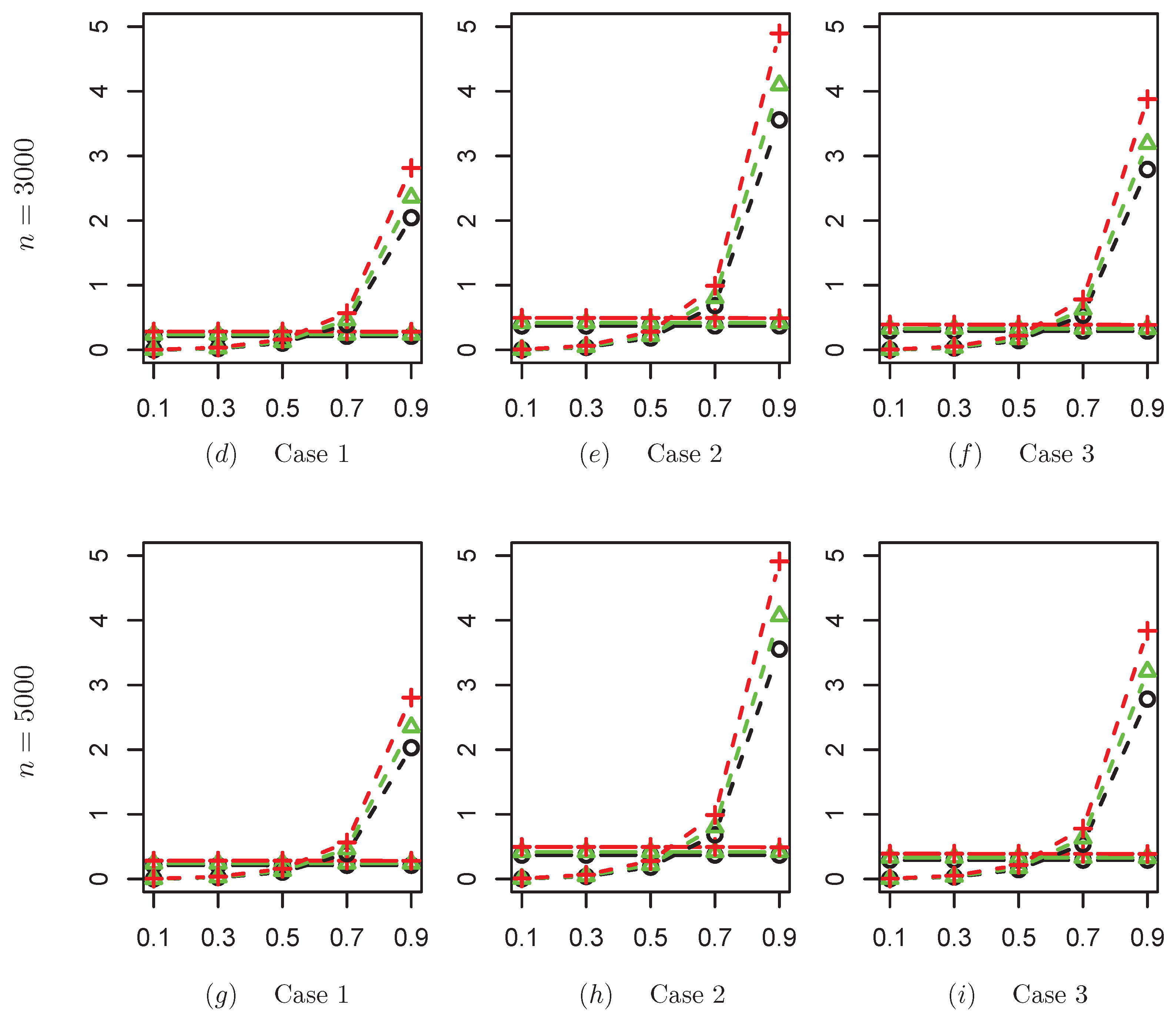
The ratio of DMSE between CQ and SCQ is firstly calculated, and the simulation results of the covariates under Case 1 are displayed in Figure 1. Since the results of the three covariate generation cases are very similar, we do not show the results of Case 2 and Case 3. The results in Figure 1 show that the ratio of DMSE estimated by CQ and SCQ is not significantly affected by changes in sample size and dimensionality. When the regression error terms are generated by symmetric distributions, i.e., the t-distribution and $Laplace$-distribution, the DMSE ratios of the regression coefficients estimators between CQ and SCQ remain above one. This indicates that SCQ has a higher precision compared with CQ, especially in the case where the difference between the lower quantile of $\tau =0.1$ and the upper quantile of $\tau =0.9$ is more obvious, and the ratio of DMSE for regression coefficients’ estimators between CQ and SCQ can reach three. When the error term is generated by the asymmetric ${\chi }^2$ distribution, the ratio of DMSE between CQ and SCQ is less than one at the low quantile level, and CQ is superior to SCQ in this case. However, the ratio of DMSE between the two methods increases as $\tau$ increases, and the ratio reaches around 10 when $\tau =0.9$. 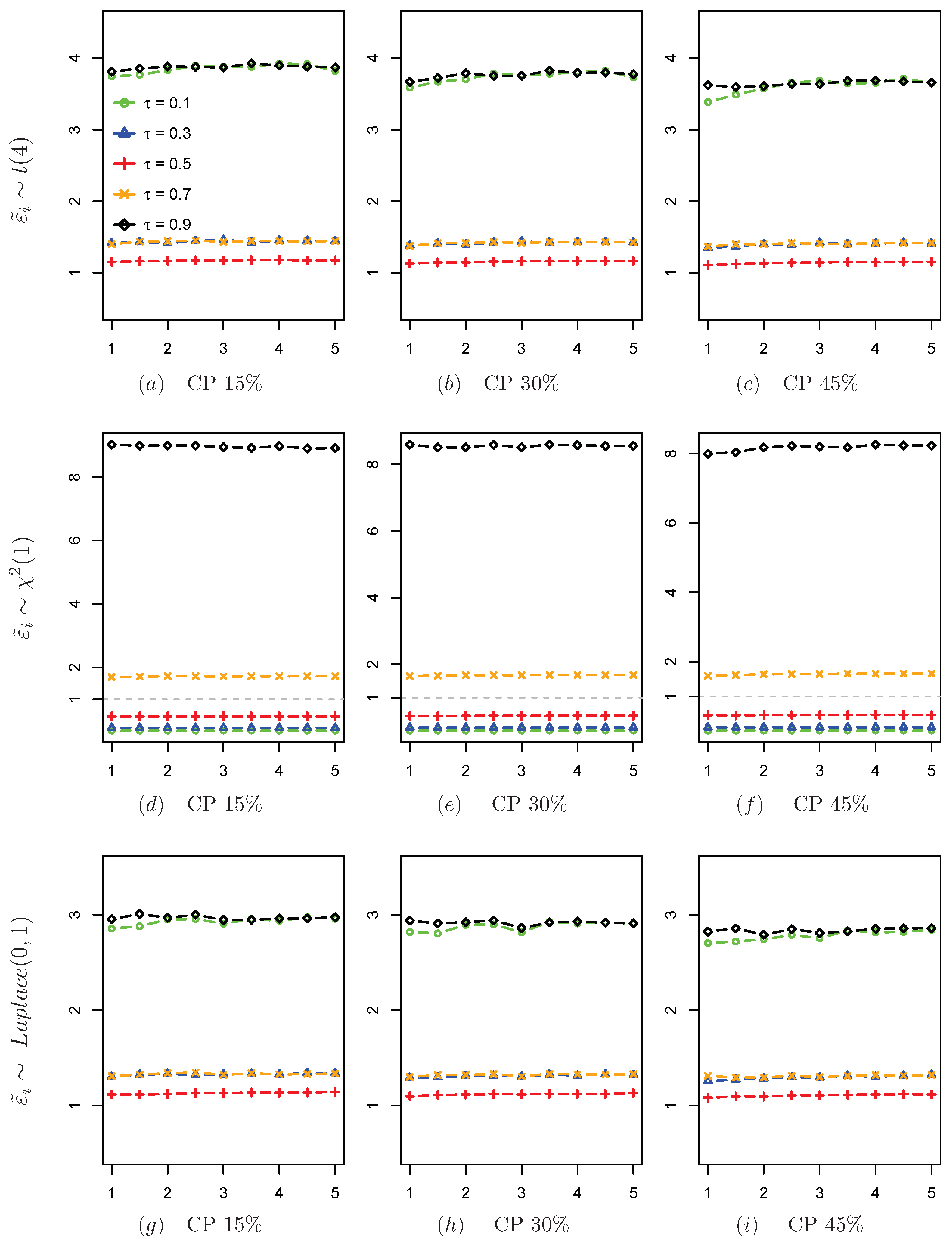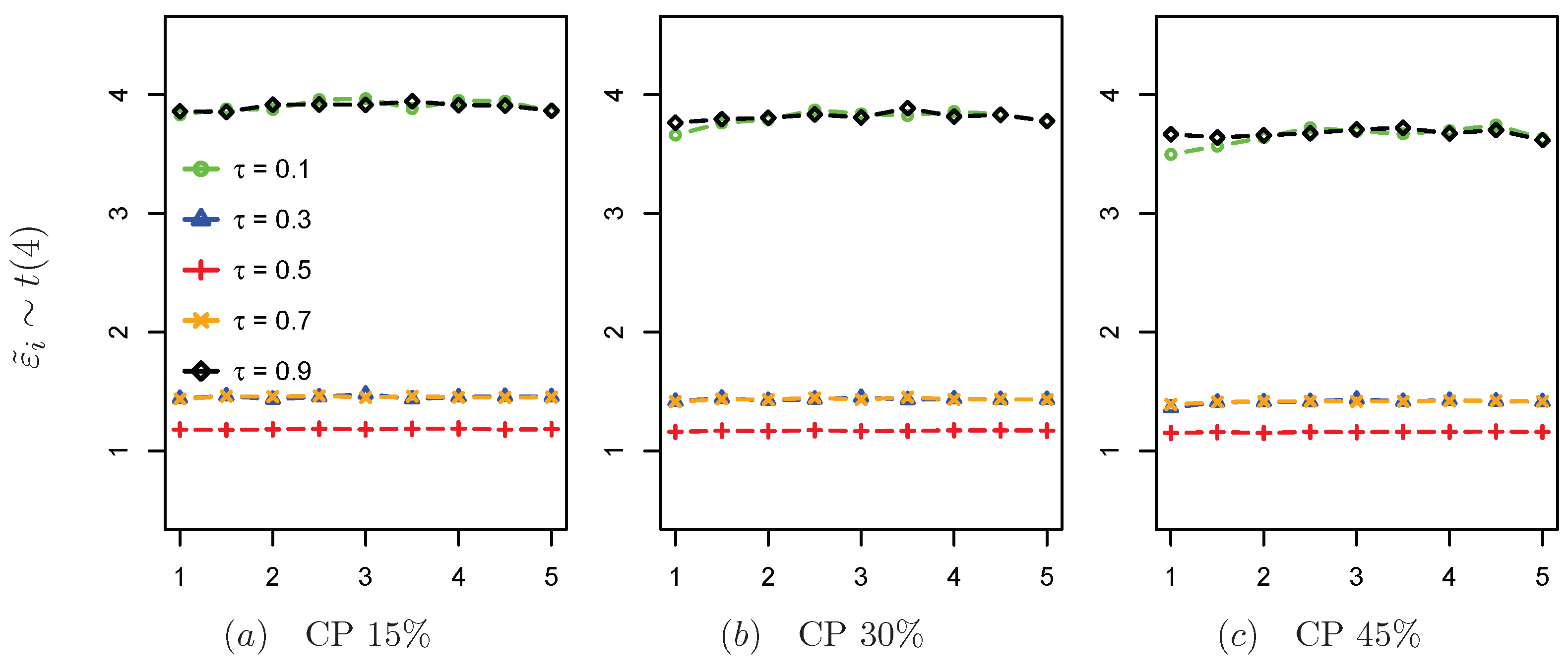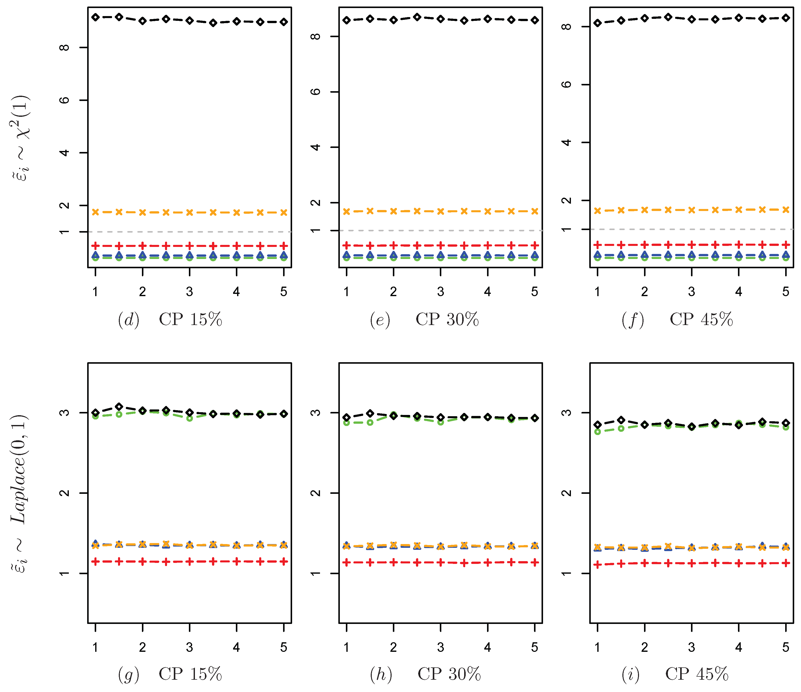In order to clarify the reason for this phenomenon, we calculate the DMSE of two estimation methods when the error term is generated by the ${\chi }^2$ distribution. As shown in Figure 2, CQ performs better when $\tau$ = 0.1. As $\tau$ increases, the DMSE of CQ increases while its growth rate gradually increases. The CQ’s DMSE is significantly higher than the SCQ’s when $\tau =0.9$, whereas the SCQ’s DMSE stabilizes at each quantile point in a straight line. The observed phenomenon aligns with its lower-dimensional counterpart, underscoring that the estimation accuracy of the CQ depends on the magnitude of $\tau$, the censoring ration of response variables and the distribution characteristics of the error term. In contrast, the estimation accuracy of the SCQ exhibits robustness against variations in these factors.

Figure 1. Estimation results for the high-dimensional model when covariate X is generated from Case 1. The horizontal coordinates of the plots indicate the sample size (in thousands), and the vertical coordinates indicate the ratio of DMSE for regression coefficients’ estimators between CQ and SCQ.

Figure 2. The DMSE of CQ and SCQ for three high-dimensional covariate generation cases when the error terms obey the ${\chi }^2$ distribution, with the horizontal coordinates denoting the different quantile levels, and the vertical axes denoting the DMSEs of the CQ and SCQ estimations scaled up by a factor of 10, where the solid line denotes the SCQ, and the dashed line denotes the CQ.

To assess the computational efficiency of the smoothing estimation, it is imperative to compare both the DMSE of CQ and SCQ estimations within the context of high-dimensional simulations, as well as the time expenditure associated with each estimation method. In Figure 3, the computational time ratios of CQ and SCQ are both greater than 1, which tends to increase with the augmentation of dimensionality and the sample size, and the computational time ratios of CQ and SCQ are more than 10 in all the cases when the sample size is $n=5000$. The results of the covariate generation in Case 2 and Case 3, which are not shown here, are similar to those in Case 1. Combined with the previous study, it is clear that, when compared to CQ, SCQ significantly decreases calculation time and increases estimation accuracy in the majority of circumstances.

Figure 3. Simulation results under the high-dimensional model when the covariates are generated from Case 1, where the horizontal coordinate denotes the sample size (in thousands), and the vertical coordinate denotes the ratio of estimated running time between CQ and SCQ.

3.4. Robustness of Smoothing Estimates

In order to compare the effects under the misspecification for the distribution of censored variables and KM estimation of censored distributions on the smoothing estimation of parameters, we choose Case 1 of the covariate generation method in the low- and high-dimensional simulations for numerical research.

When the sample size is 200, the model coefficients are estimated using convolutional smoothing after assuming that the distribution of the censored variables is misclassified as Normal, Weibull, and Lognormal, and using the KM estimation of G with different conditions of $\tau$ quantiles, censoring proportions, and error terms. The simulation in Table 4 shows that the smoothing estimation using the misclassified distribution of the censored variables is more robust than the smoothing estimation using the KM estimation to estimate the distribution of the censored variables. Similar results are obtained for a sample size of 3000, as shown in Table 5.

Table 4. Smoothing estimators of regression model parameters after misclassifying the distribution of censored variables as Normal, Weibull, and Lognormal, and after estimating G using KM estimation. The covariate X in the low-dimensional model is generated from Case 1, where the values in columns 2–13 are DMSE ×${10}^5$. The sample size of the simulation is fixed at 200.

$\mathit{\tau }$	Normal			Weibull			Lognormal			KM Estimation
	15%	30%	45%	15%	30%	45%	15%	30%	45%	15%	30%	45%
	${\tilde{\epsilon }}_i\sim t\left(4\right)$
0.1	588	766	991	567	722	938	564	709	916	1366	1404	1448
0.3	554	682	861	552	677	858	552	677	858	1158	1192	1203
0.5	537	644	808	543	655	823	545	660	832	1123	1128	1157
0.7	524	618	774	536	639	800	539	648	815	1037	1051	1100
0.9	511	594	754	529	620	776	534	631	793	976	1000	1091
	${\tilde{\epsilon }}_i\sim {\chi }^2\left(1\right)$
0.1	808	1006	1270	793	974	1227	791	966	1212	1786	1847	1982
0.3	803	995	1250	790	969	1215	789	962	1202	1788	1810	1902
0.5	792	969	1212	785	955	1191	785	953	1185	1716	1778	1856
0.7	772	922	1150	776	929	1151	778	933	1155	1521	1684	1820
0.9	740	858	1076	759	886	1088	765	898	1102	1305	1409	1472
	${\tilde{\epsilon }}_i\sim Laplace(0,1)$
0.1	1213	1671	2138	1160	1560	2047	1151	1525	1999	1778	2023	2348
0.3	1141	1472	1835	1126	1451	1851	1125	1444	1851	1370	1595	1897
0.5	1102	1372	1695	1106	1392	1754	1110	1400	1777	1208	1434	1731
0.7	1071	1295	1593	1092	1344	1678	1099	1363	1717	1116	1326	1609
0.9	1034	1215	1513	1072	1285	1604	1083	1314	1655	1078	1304	1598

Table 5. Smoothing estimates of regression model parameters after misclassifying the distribution of censored variables as Normal, Weibull, and Lognormal, and after estimating G using KM estimation. The covariate X in the high-dimensional model is generated from Case 1, where the values in columns 2–13 are DMSE ×${10}^4$. The sample size of the simulation is fixed at 3000.

$\mathit{\tau }$	Normal			Weibull			Lognormal			KM Estimation
	15%	30%	45%	15%	30%	45%	15%	30%	45%	15%	30%	45%
	${\tilde{\epsilon }}_i\sim t\left(4\right)$
0.1	1962	2272	2891	1952	2270	2945	2020	2274	2965	2634	3593	4324
0.3	1951	2260	2937	1940	2258	2925	2022	2263	2943	2570	3532	4343
0.5	1945	2253	2891	1935	2251	2913	2026	2255	2936	2489	3459	4373
0.7	1943	2249	2902	1933	2247	2900	2019	2253	2931	2394	3381	4273
0.9	1943	2239	2892	1932	2236	2876	2013	2239	2912	2369	3306	4172
	${\tilde{\epsilon }}_i\sim {\chi }^2\left(1\right)$
0.1	2411	2427	2855	2391	2415	2844	2421	2445	2868	3605	3613	4105
0.3	2402	2439	2864	2392	2437	2844	2416	2448	2885	3390	3438	4035
0.5	2421	2435	2851	2391	2426	2842	2432	2447	2865	3308	3350	4062
0.7	2412	2446	2854	2392	2434	2843	2425	2465	2864	3307	3353	3955
0.9	2409	2442	2832	2390	2431	2825	2413	2444	2850	3262	3271	4009
	${\tilde{\epsilon }}_i\sim Laplace(0,1)$
0.1	3857	4742	6153	3846	4739	6143	3861	4757	6165	3640	4442	5388
0.3	3840	4724	6096	3834	4711	6085	3853	4742	6101	3602	4349	5403
0.5	3838	4710	6051	3827	4692	6045	3841	4740	6067	3728	4252	5332
0.7	3835	4682	6018	3819	4675	6006	3851	4695	6024	3789	4169	5236
0.9	3834	4662	5963	3816	4654	5951	3849	4686	5975	3610	4097	5195

The simulation shows that although there is a possibility of mis-setting in estimating the parameters of the distribution of the censored variables by using $\widehat{G}(·)=G(·,{\widehat{\mathit{\theta }}}_n)$, this method is better and more robust than the smoothing of regression models after estimating the distribution of the censored variables by using the KM estimation. During the simulation process, it is also found in Table 4 and Table 5 that when the censored variables are estimated in different distribution forms, the smoothing estimation errors of the model coefficients exhibit a minimal degree of variation, and the estimation accuracy is higher than that of using KM estimation to estimate the distribution of the censored variables and then carry out the smoothing estimation. Regarding computational efficiency, the smoothing estimation method, when applied in scenarios of distributional misclassification, demonstrates a running time ratio to the SCQ that fluctuates within the range of 0.9 to 1.1. In contrast, the smoothing estimation method, once preceded by the KM estimation, incurs a significantly extended running time.

4. Discussion

In the smoothing estimation of censored quantile regression models, the distribution of the censored variables is usually unknown. The problem of the unknown distribution of the censored variables can be solved by estimating the density function of the censored variables through existing nonparametric methods, then determining the type of the censored distribution using the goodness-of-fit test, and accessing the unknown parameters in the distribution using the great likelihood method. In the numerical simulation, this paper also discusses using such a method to fit the unknown censored distribution $G(·)$ to estimate $\widehat{G}(·)=G(·,{\widehat{\mathit{\theta }}}_n)$, and then estimate the regression parameter $\mathit{\beta }$.

We also discuss the parametric smoothing estimation method in the case of misspecification of the distribution of the censored variables, and compare it with the smoothing estimation method of the parameters after estimating the distribution of the censored variables $\widehat{G}(·)$ with KM estimation. The simulation results show that the smoothing estimation method is still more robust than the method of estimating the distribution of censored variables $\widehat{G}(·)$ with KM estimation even if there is a misspecification in the estimation of the distribution of the censored variables. Meanwhile, the smoothing estimation method is more robust than the classical censored quantile regression model.

Our research has certain limitations and there are some issues that need to be further explored. Firstly, we have performed some analysis and research on parameter smoothing estimation for quantile linear models; moreover, we can plan further research on parameter estimation and interval estimation for complex models such as generalized linear models. Secondly, our proof is based on the assumption that the form of censored distribution is known, and the theoretical proof by using a nonparametric model to estimate the censored distribution is still a challenging task. This requires understanding and knowledge in the theory of nonparametric statistics and probability limits.

5. Conclusions

In this paper, a convolutional smoothing estimation method for the censored quantile regression model is proposed to address the problem that the loss function is not derivable. Our method associates the convolutional smoothing estimation with the loss function of censored quantile regression, which is quadratically derivable, compared with the classical censored quantile regression estimation. Moreover, the smoothing estimation method for censored quantile regression models improves the estimation accuracy, computational speed, and robustness over the classical parameter estimation method. The contribution and significance of this paper can be summarized as follows:

• The method establishes links between the convolutional smoothing method and the loss function of the censored quantile regression model, and the use of the non-negative kernel function ensures that the smoothed loss function is quadratically derivable and globally convex, which can be used to improve the computational speed by using the gradient-based iterative algorithm.
• Theoretically, we characterize the bias of the smoothing estimation for censored quantile regression and establish the convergence rate, Bahadur–Kiefer representation, and Berry–Esseen upper bound of the smoothing estimation under high-dimensional and large-sample conditions.
• The numerical simulation shows that the smoothing estimation method greatly reduces the computation time and improves the estimation accuracy in most cases, compared with the classical parameter estimation. In addition, the accuracy of CQ estimator is highly dependent on $\tau$, censoring ratio(CP), and the distribution of error term, but the SCQ estimation is robust to these factors.