Estimating the Relative Risks of Spatial Clusters Using a Predictor–Corrector Method

Abstract

Spatial, temporal, and space–time scan statistics can be used for geographical surveillance, identifying temporal and spatial patterns, and detecting outliers. While statistical cluster analysis is a valuable tool for identifying patterns, optimizing resource allocation, and supporting decision-making, accurately predicting future spatial clusters remains a significant challenge. Given the known relative risks of spatial clusters over the past k time intervals, the main objective of the present study is to predict the relative risks for the subsequent interval, $k+1$. Building on our prior research, we propose a predictive Markov chain model with an embedded corrector component. This corrector utilizes either multiple linear regression or an exponential smoothing method, selecting the one that minimizes the relative distance between the observed and predicted values in the k-th interval. To test the proposed method, we first calculated the relative risks of statistically significant spatial clusters of COVID-19 mortality in the U.S. over seven time intervals from May 2020 to March 2023. Then, for each time interval, we selected the top 25 clusters with the highest relative risks and iteratively predicted the relative risks of clusters from intervals three to seven. The predictive accuracies ranged from moderate to high, indicating the potential applicability of this method for predictive disease analytic and future pandemic preparedness.

1. Introduction

The emergence of COVID-19 highlighted the critical need for precise spatial and temporal surveillance of infectious diseases, especially in densely populated or vulnerable regions. The spatial scan statistic has proven essential for identifying disease clusters in public health data and helping authorities detect, respond to, and mitigate outbreaks. It was first proposed by Kulldorff [1] and subsequently developed in various studies [2,3]. This method, using circular and, later, elliptic scanning windows [4], efficiently identifies clusters without prior information on the disease’s distribution, providing a robust framework for various applications, from infectious diseases to cancer epidemiology [5,6]. Kulldorff’s elliptic spatial scan statistics address the limitations of circular windows, particularly in urban environments, where the population density and movement patterns are uneven [4].

Additional advancements include the weighted normal spatial scan statistic, which accommodates heterogeneous population data, enabling more precise detection in demographically diverse regions [3,7]. Studies on COVID-19, for instance, have applied these techniques to uncover spatial variations and emerging hot spots within urban settings, providing critical insights into the pandemic’s dynamics [8,9,10,11,12]. Another study [13], explored how these spatial methods facilitated response coordination across countries, reflecting the adaptability of spatial scan statistics in different geographic contexts and for different disease typologies. Additionally, the multivariate scan statistic extends the traditional models to analyze multiple data types simultaneously, thereby improving the accuracy of surveillance of multifactorial diseases [2]. The utility of Monte Carlo hypothesis testing, as demonstrated in [14] and further refined for power analysis by [15], is integral to validating spatial clusters, adding another layer of reliability to these models.

These spatial methodologies have also shown efficacy in tracking non-COVID infectious diseases. For example, space–time models applied to airborne diseases like H7N9 influenza [16,17,18] have demonstrated their utility in understanding the disease spread and preparing targeted interventions. Furthermore, Souris et al. [19] illustrated the application of these tools in poultry farms, identifying the avian influenza re-emergence risks across human and animal health sectors (see also [20,21]).

In healthcare-associated infection settings, these models have helped detect and control outbreaks, as shown in studies on methicillin-resistant Staphylococcus aureus [22] and carbapenemase-producing Klebsiella pneumoniae [23]. By incorporating real-time data, these systems provide timely alerts, allowing healthcare providers to implement interventions more rapidly [24]. Syndromic surveillance adaptations, which emerged from studies on anthrax preparedness by [25] and subsequent research by [26], underscore the proactive role of these systems in modern epidemiological surveillance.

The spatial scan statistic and its derivatives have been instrumental across public health, responding to infectious diseases, environmental exposure, and even syndromic surveillance scenarios. These tools can become even more powerful when applied to prediction, as predictive applications extend the utility of spatial cluster analysis beyond retrospective assessments. The main question is whether predictive methods can be merged with these tools to identify regions at heightened risk of future disease spread, anticipate the healthcare resource requirements, and guide targeted interventions in real time, enabling decision-makers to allocate resources more effectively. In this paper, we aim to test the applicability of a predictor–corrector method to the relative risks resulting from a spatial cluster analysis of k time intervals for predicting the relative risks in the time interval $k+1$. In particular, assuming that the relative risks of spatial clusters are known for the past k time intervals, we are interested in predicting the relative risks of these spatial clusters in the time interval $k+1.$ Based on our previous work [27], we propose a Markov chain model with an embedded corrector. The corrector is either multiple linear regression or exponential smoothing, whichever allows for a shorter relative distance between the observed and predicted values in interval k.

Predicting the relative risks in spatial clusters could serve as an early warning system for areas at increased mortality risk, which is especially valuable for addressing resource allocation and intervention planning in critical periods. We use the U.S. COVID-19 mortality data [28] to evaluate this approach and assess whether this method can accurately forecast the relative risks in clusters with significant mortality.

The remainder of this paper is organized as follows. Section 2 provides details on the data, the SaTScan method [29], and the results of our spatial cluster analysis. Section 3 introduces the predictor–corrector method, while Section 4 applies this method to the U.S. COVID-19 mortality data over six time intervals, with the goal of predicting the relative risks in the seventh time interval. Finally, Section 5 discusses the results and limitations of the present work, as well as potential directions for future research.

2. Retrospective Analysis of Spatial Clusters

2.1. Overview

We employed a retrospective spatial analysis of COVID-19 clusters across the United States by examining how the case distributions correlate with population density. Utilizing a Poisson-based spatial scanning model, we identified clusters by employing a cylindrical scanning window to capture areas of heightened risk relative to their surrounding regions. The analysis applied likelihood ratio testing to detect significant spatial clusters, with primary and secondary clusters reported based on statistical significance. Monte Carlo simulations were used to validate the results, offering insights into the geographic spread and demographic impact of COVID-19 across different communities in the U.S.

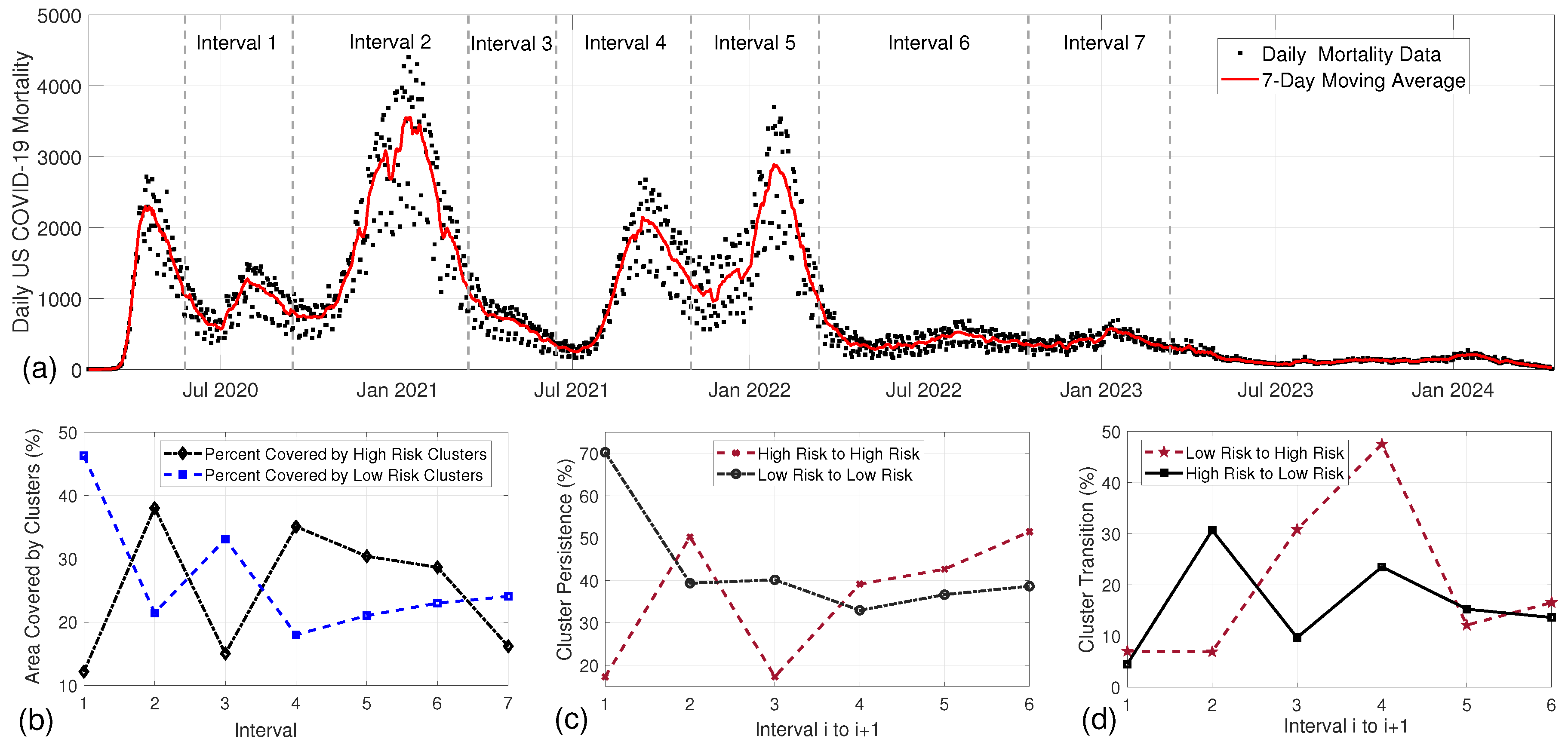
2.2. U.S. COVID-19 Mortality Data

We obtained COVID-19 mortality data for the United States from The New York Times, which provides daily records of COVID-19 deaths from February 2020 onward. These data are publicly available at [28].

The dataset reports the daily COVID-19 deaths across all U.S. states and territories. In many states, health departments reconcile these records with death certificates, omitting deaths where COVID-19 was not the cause of death. Following this protocol, non-COVID-19 deaths were removed from the dataset when there was confirmation that COVID-19 was not the cause, specifically in cases of homicide, suicide, car accidents, or drug overdoses. Details of these adjustments can be found in [28].

To examine significant variations in COVID-19 mortality trends, we focused on data spanning from 24 May 2020 to 12 March 2023. We divided this period into seven time intervals to analyze the trends within consistent segments of time: 24 May 2020–13 September 2020; 13 September 2020–14 March 2021; 14 March 2021–13 June 2021; 13 June 2021–31 October 2021; 31 October 2021–13 March 2022; 13 March 2022–16 October 2022; and 16 October 2022–12 March 2023. Each interval represents a critical phase in the pandemic, allowing us to study the temporal fluctuations in COVID-19-related mortality rates (see

Table 1. U.S. COVID-19 control and preventive measures by time interval.

Interval	Variants	Control and Preventive Measures	Refs.
1. 5/24/2020–9/13/2020	Original strain (Wuhan)	Social distancing measures, use of face masks, limitations on gatherings, travel restrictions	[31,32]
2. 9/13/2020–3/14/2021	D614G variant	Expanded mask mandates, introduction of COVID-19 vaccines (Pfizer, Moderna), enhanced testing and contact tracing	[33,34]
3. 3/14/2021–6/13/202	Alpha variant (B.1.1.7)	Vaccination campaigns ramped up, continued mask-wearing in high-transmission areas	[35,36]
4. 6/13/2021–10/31/2021	Alpha variant predominant	CDC recommendations for vaccinated individuals, return to in-person learning in colleges and schools, ongoing vaccination efforts	[36,37]
5. 10/31/2021–3/13/2022	Delta variant (B.1.617.2)	Booster shots recommended, reinstated mask mandates in certain areas, increased indoor venue capacity restrictions	[37,38]
6. 3/13/2022–10/16/2022	Omicron variant (B.1.1.529)	Vaccination updates including boosters, recommendations for masks in crowded indoor settings, continued public health surveillance	[31,37]
7. 10/16/2022–3/12/2023	Omicron subvariants (BA.1, BA.2)	Focus on public health awareness campaigns, emphasis on personal responsibility regarding health measures	[39,40]

for a summary). Specifically, these intervals were selected based on the emergence of new SARS-CoV-2 variants, which played a pivotal role in shaping the trajectory of the pandemic. This approach aimed to capture virological and epidemiological shifts corresponding to significant phases of the outbreak. Each interval, except the third, includes at least one peak in COVID-19 mortality within the United States (see Figure 2a). The third interval corresponds to the emergence of the Alpha variant, which did not result in a mortality peak during this period but contributed to a significant peak in the subsequent interval. While this method highlights the variant-driven dynamics, we acknowledge that alternative approaches, such as structural change detection methods [30], could potentially offer a data-driven determination of breakpoints. Incorporating such methods into future studies could refine the interval selection process further and enhance the robustness of the predictive modeling.

2.3. Spatial Statistical Scan

To analyze the geographical distribution of COVID-19 cases adjusted for population demographics, we applied a Poisson model. Our spatial analysis utilized a cylindrical scanning approach, with a moving circular base representing the spatial dimension, and set a maximum cluster size of 25% of the population at risk to prevent excessively large clusters. This approach created numerous overlapping windows of varying sizes, allowing for full coverage of the study area. Each window was considered a potential cluster. Under the null hypothesis $H_0$, the COVID-19 risk is uniform inside and outside the scanning window, while the alternative hypothesis $H_a$ suggests a higher risk within the window. Each cylinder expanded up to a preset upper limit on cluster size. To identify clusters, we applied a likelihood ratio test.

The likelihood ratio ${\displaystyle \frac{L\left(C\right)}{L_0}}$ is calculated by

$${\displaystyle \frac{L\left(C\right)}{L_0}}={\displaystyle \frac{{\left(\frac{n_c}{\mu \left(c\right)}\right)}^{n_c}{\left(\frac{N-n_c}{N-\mu \left(c\right)}\right)}^{N-n_c}}{{\left(\frac{N}{\mu \left(T\right)}\right)}^N}},$$

(1)

where $L\left(C\right)$ is the maximum likelihood for the cylinder based on the observed cases $n_c$ and the expected cases $\mu \left(c\right)$ within the window. Here, $L_0$ is the likelihood under the null hypothesis, N is the total cases observed in the U.S. for each time interval, and $\mu \left(T\right)$ represents the total expected cases. A likelihood ratio greater than one indicated that the number of cases observed exceeded expectations. The cluster with the highest likelihood was labeled the primary cluster, while other clusters were reported if they achieved significance at $p<0.05$. The p-values for space–time clusters were determined through Monte Carlo simulations, using randomized iterations of the data to assess statistical significance [29].

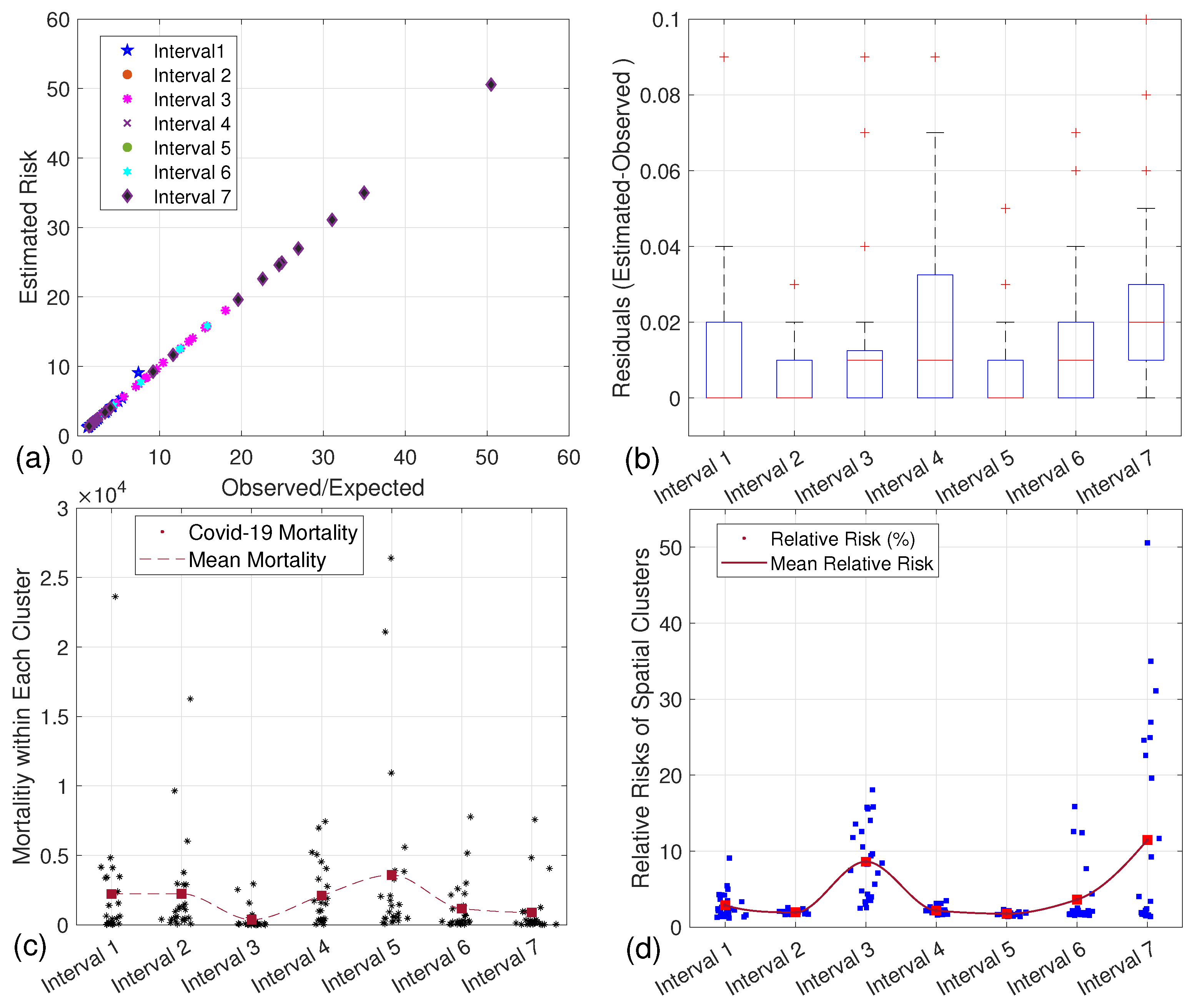
2.4. Significant Clusters Identified

Figure 1 illustrates the significant spatial clusters of COVID-19 mortality across the United States. High-risk clusters, characterized by a relative risk greater than one, are represented as red circles, while low-risk clusters, with a relative risk less than one, are indicated by blue circles. Panel (a) shows the significant spatial clusters for the entire study period; however, it may not adequately reflect the temporal changes across the defined time intervals from 1 to 7. Panels (b) through (h) correspond to the spatial data associated with intervals 1 through 7, respectively. Panel (b) shows that significant high-risk clusters were initially concentrated in the southern regions of the U.S. As shown in panel (c), these high-risk clusters extend across much of the country, with notable exceptions of certain areas in the East and Northwest, which may be attributed to lower vaccination rates. Panel (d) illustrates the impact of extensive vaccination efforts, which have proven to be substantially effective. The emergence of the Delta variant is notable in panel (e), demonstrating its influence on the increased mortality trends. The effectiveness of vaccination updates and booster shots is evident in panel (f) when it is compared with panel (e). Panel (g) indicates that the significance of the Omicron variant has become pronounced in the central regions of the U.S. Finally, panel (h) reveals a substantial reduction in the number of significant high-risk clusters, underscoring the impact of vaccination and public health interventions on COVID-19 mortality rates.

Figure 2 shows the dynamics of the COVID-19 mortality trends and the geographical distribution of risk clusters in the U.S., highlighting key patterns in mortality fluctuations, spatial risk persistence, and transitions between risk classifications. Panel (a) illustrates the time series of COVID-19-related mortality in the U.S. from 24 May 2020 to 12 March 2023, segmented into seven distinct periods. Panel (b) shows the percentage of the area of the U.S. covered by significant high-risk clusters (i.e., with a relative risk greater than 1) and low-risk clusters (i.e., with a relative risk less than 1) for each of the seven intervals. It suggests that both high-risk and low-risk clusters may gradually reach an equilibrium below 20% of the area of the U.S., indicating a stable distribution of risk across the country. Panel (c) examines the persistence of high-risk and low-risk clusters from time interval i to interval $i+1$. It demonstrates that approximately 45% of areas classified as high-risk and about 40% of areas classified as low-risk maintain their status, particularly from time interval 5 onward, suggesting a notable consistency in the spatial risk distribution over time. Panel (d) illustrates the percent transition of clusters from high-risk to low-risk and vice versa between consecutive intervals. This transition appears to stabilize around 15%, indicating a moderate but consistent change in the risk classification of certain areas over the specified periods.

Table 2. Summary statistics of spatial clusters of a high risk and a low risk of COVID-19 mortality across intervals 1–7, showing the number of clusters, U.S. areas covered by each group with the percent areas shown inside the parentheses, and the overlap between the high risk and low risk clusters. Note that areas are measured in square kilometers with the total U.S. area of 9,629,091 km².

Interval	High-Risk	Low-Risk	Area of High Risk	Area of Low Risk	Overlap Area	Total Area
1	25	38	1,170,531.55 (12.16%)	4,457,499.54 (46.29%)	4830.30 (0.05%)	5,623,200.79 (58.40%)
2	38	34	3,661,450.98 (38.02%)	2,065,006.01 (21.45%)	7781.26 (0.08%)	5,718,675.73 (59.39%)
3	40	39	1,447,800.92 (15.04%)	3,189,789.31 (33.13%)	5915.07 (0.06%)	4,631,675.16 (48.10%)
4	30	25	3,379,836.76 (35.10%)	1,733,777.69 (18.01%)	24,583.89 (0.26%)	5,089,030.56 (52.85%)
5	29	36	2,928,563.46 (30.41%)	2,024,862.64 (21.03%)	14,785.95 (0.15%)	4,938,640.15 (51.29%)
6	29	25	2,760,890.45 (28.67%)	2,214,642.66 (23.00%)	3259.16 (0.03%)	4,972,273.95 (51.64%)
7	28	30	1,556,809.44 (16.17%)	2,316,998.49 (24.06%)	5328.31 (0.06%)	3,868,479.62 (40.17%)

presents a detailed summary of high-risk and low-risk spatial clusters of COVID-19 mortality across intervals 1 through 7. The second and third columns list the number of high-risk and low-risk clusters identified in each interval. Columns 4 through 7 provide the percentage of the total area of the U.S. covered by these clusters. Since the spatial clusters span both land and water, incorporating the US total area provides a more accurate estimation of the percent areas covered by the high risk and a low risk spatial clusters for each time interval. Hence, we used total U.S. area of 9,629,091 km² instead of US land area 9,147,590 km². Notably, in intervals 2 and 4, high-risk clusters encompassed more than 35% of its area.

Table 3. Estimated transitions between and persistence rates of high-risk and low-risk clusters of COVID-19 mortality across consecutive intervals. The percent overlaps have been shown inside the parentheses. The first percentage represents the overlap of clusters from interval i with those in interval $i+1$, and the second indicates the overlap of clusters in interval $i+1$ with interval i.

Intervals	High-Risk Overlap	Low-Risk Overlap	High–Low Transition	Low–High Transition
1 → 2	630,606 (53.87%, 17.22%)	1,451,535 (32.56%, 70.29%)	93,533 (7.99%, 4.53%)	1,311,032 (29.41%, 35.81%)
2 → 3	727,798 (19.88%, 50.27%)	1,255,175 (60.78%, 39.35%)	979,045 (26.74%, 30.69%)	100,420 (4.86%, 6.94%)
3 → 4	583,839 (40.33%, 17.27%)	696,469 (21.83%, 40.17%)	168,040 (11.61%, 9.69%)	1,042,772 (32.69%, 30.85%)
4 → 5	1,146,392 (33.92%, 39.15%)	667,377 (38.49%, 32.96%)	476,609 (14.10%, 23.54%)	1,391,524 (21.28%, 12.60%)
5 → 6	1,178,061 (40.23%, 42.67%)	811,950 (40.09%, 36.66%)	337,960 (11.54%, 15.26%)	335,357 (16.56%, 12.15%)
6 → 7	802,151 (29.05%, 51.53%)	895,447 (40.43%, 38.65%)	315,871 (11.44%, 13.63%)	257,680 (11.64%, 16.55%)

details the transitions between clusters with a high risk and low risk of COVID-19 mortality, as well as the persistence of these clusters across the intervals from i to $i+1$. Two percentages are provided: the first represents the overlap of clusters from interval i with those in interval $i+1$, and the second indicates the overlap of clusters in interval $i+1$ with interval i. Notably, the values approach steady-state levels over time.

Figure 3 represents the accuracy of the spatial clusters identified. Panel (a) shows the observed-to-expected mortality counts plotted against the estimated relative risk for intervals 1–7, which shows high accuracies of the estimates; panel (b) provides box plots of the residuals, indicating low residuals; panel (c) illustrates the mortality data within each identified cluster, giving a localized perspective on the mortality distribution; and panel (d) displays the estimated relative risks associated with the spatial clusters for each interval, showing the changes in risk levels over time. The observed-to-expected mortality counts and the relative risks of significant spatial clusters are available in Supplementary Materials Table S1 and Table S2, respectively.

3. Modeling Mortality Risk Prediction

3.1. The Markov Chain Model

In tackling the challenge of integrating the entire cluster search and prediction process into a manageable model grounded in a rigorous statistical analysis, we propose that analyzing the trends in the transition probabilities across the observed clusters over k intervals could enhance the accuracy of our predictions for interval $k+1$. Given that k is relatively small (between 5 and 10), we employ a predictor–corrector method explained below. The predictor utilizes a Markov chain model [41,42], while the corrector optimally chooses between multiple linear regression and exponential smoothing methods based on the distance between the transition matrices, aiming for an effective prediction of the clusters in interval $k+1$.

Our approach starts with the establishment of the initial datasets, labeled $T_i$, with each representing a specific time interval i. As the pandemic progresses, datasets $T_1,T_2,T_3,$ and so on are created based on the defined time intervals, forming a sequence that captures different phases of the pandemic. The duration of each interval can be customized by the user to align with significant variations identified in the time series data. The collection $T_{k+1}$ denotes the next set of real data gathered at a subsequent interval. Our goal is to predict the parameters of this new collection $T_{k+1}$ using insights from the preceding datasets $T_1,T_2,\dots ,T_k$.

Traditionally, predictions for mortality rates have relied solely on the most recent dataset, $T_k$. However, we recognize that the characteristics of the upcoming dataset $T_{k+1}$ may differ from those represented by $T_k$. To improve the predictive accuracy, we advocate for a broader analysis of the trends in the transition probabilities observed across the series of datasets $T_1,T_2,\dots ,T_k$.

Understanding the patterns and shifts in the transition probabilities over time can provide valuable insights into the evolving dynamics of the pandemic. By examining how these probabilities change, we aim to capture underlying trends that may enhance the accuracy of predicting the parameters for the next dataset, $T_{k+1}$. This approach contrasts with conventional methods, suggesting that a more nuanced analysis of historical data could lead to a more robust and reliable predictive model for mortality rates in the ongoing fight against COVID-19.

3.2. Estimating the Parameters of $T_{k+1}$

Let $T_{k+1}^{*}$ represent the prediction for $T_{k+1}$. Predicting $T_1$ is impractical because there are no initial data available before $T_1$. Similarly, predicting $T_2$ is challenging due to the presence of only one preceding dataset, which does not provide sufficient patterns or trends. However, $T_k^{*}$ can be predicted for $k>2$ using the datasets $T_1\dots T_{k-1}$. This means that historical data can be maintained as prediction chains throughout the data collection process. More importantly, since predictions are made for each dataset as it becomes available, any inaccurate predictions can be discarded, offering valuable feedback on the quality of the predictive process.

Our proposed method corrects the Markov chain prediction of $T_{k+1}$ utilizing either multiple linear regression or exponential smoothing at each iteration k. The predictor, denoted as $T_{k+1}^{*}$, is formulated as follows:

$$T_{k+1}^{*}={\alpha }^{*}{T}_k+(1-{\alpha }^{*})T_k^{*},$$

(2)

which is a weighted sum between a “good corrector” $T_k^{*}$ and data $T_k$. The “good corrector” ${T^{*}}_k$ of $T_k$ is based on the transition matrices from previous datasets $T_1,T_2,\dots ,T_{k-1}$, whereas the predictor is given as ${\alpha }^{*}{T}_k$. Specifically, let ${\widehat{T}}_k$ be a predictor of $T_k$ determined through multiple linear regression, and let ${\tilde{T}}_k$ be a predictor of $T_k$ determined via exponential smoothing. ${\tilde{T}}_k$ depends on ${\alpha }^{*}$, an optimal value satisfying $0<{\alpha }^{*}<1$, and is determined by

$$\sum _{i=3}^{k}d({\tilde{T}}_i\left({\alpha }^{*}\right),T_i)=\underset{0<a<1}{min}\left\{\sum _{i=3}^{k}d({\tilde{T}}_i\left(\alpha \right),T_i)\right\}.$$

(3)

$T_k^{*}$ is chosen as ${\tilde{T}}_k$ or ${\widehat{T}}_k$ using the criterion

$$d(T_k^{*},T_k)=min\{d({\widehat{T}}_k,T_k),d({\tilde{T}}_k,T_k)\},$$

(4)

where $d(T_k^{*},T_k)$ denotes the distance from transition matrix $T_k^{*}$ to matrix $T_k$. We will use a distance measure of the form

$$d(T_k^{*},T_k)=\sum _m\sum _n{\displaystyle \frac{\left|\right(T_k^{*}(m,n)-T_k(m,n)\left)\right|}{T_k(m,n)+1}}.$$

(5)

Here, m represents the matrix row index, while n denotes the matrix column index. This distance metric accounts for relative differences rather than absolute differences. See Ref. [43] for more details.

As a result, we derive the parameters of $T_{k+1}^{*}$ by utilizing the previous dataset $T_k$, which is established with real data, and $T_k^{*}$, a predictor for $T_k$ that encapsulates historical information from the datasets $T_1,\dots ,T_{k-1}$. Throughout this process, we eventually obtain the actual $T_{k+1}$ and compare it to our estimate $T_{k+1}^{*}$ using the aforementioned distance measure. This method allows us to assess the accuracy of our predictions with each successive data collection. Importantly, the distance measure can reveal whether certain datasets are outliers for various reasons, enabling us to exclude those data points from our analysis.

The ultimate goal is to determine $T_{k+1}^{*}$, for which no corresponding $T_{k+1}$ will be available, especially when $T_k$ represents the final data collection before making a prediction. Thus, $T_{k+1}^{*}$ serves as our prediction for practical use, representing our estimate in the absence of actual observed data for $T_{k+1}$. The next subsection provides additional details.

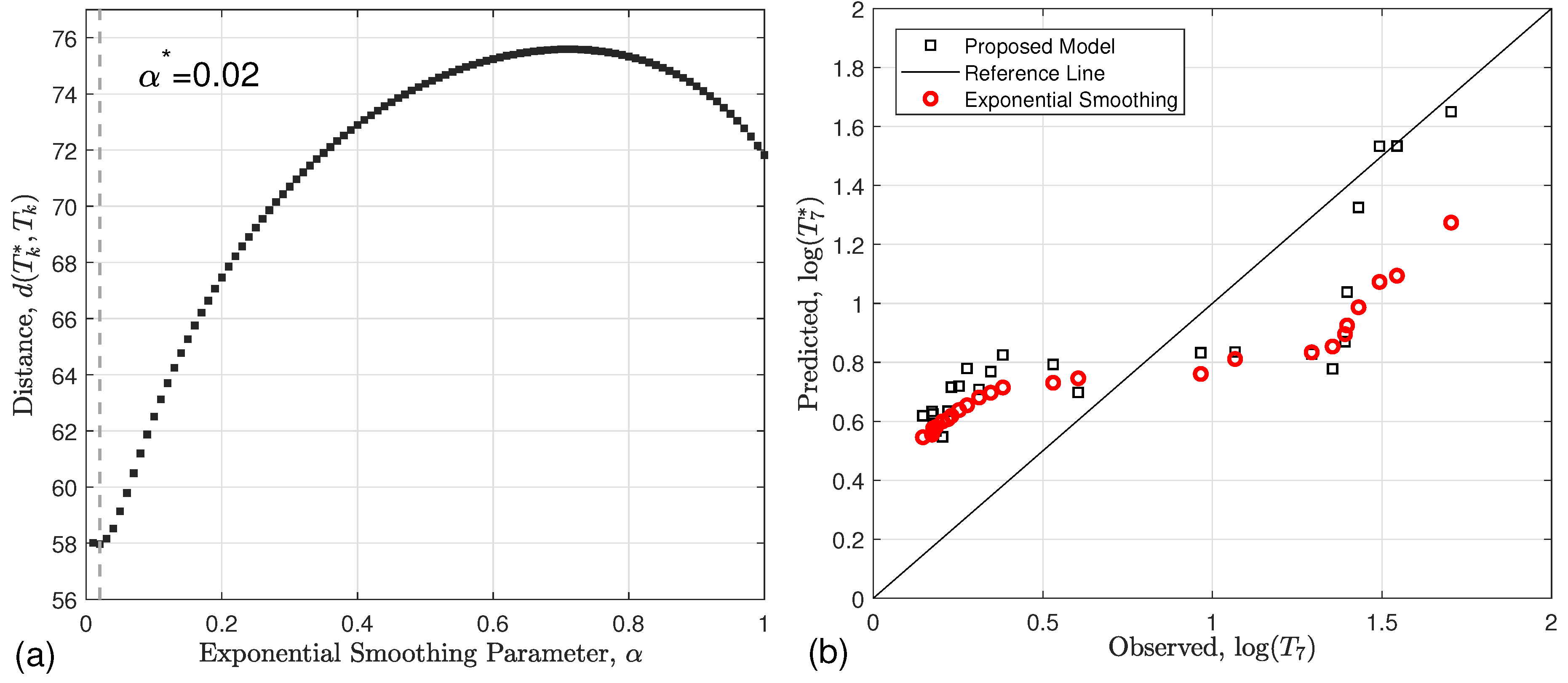
3.3. Predictors of the Transition Matrix $T_{k+1}^{*}$

We employ one of two methods to predict $T_{k+1}^{*}$ based on the transition matrices $T_1,T_2,\dots ,T_k$. The value ${\tilde{T}}_k$ is calculated using exponential smoothing, while ${\widehat{T}}_k$ is obtained through multiple linear regression. The method that results in the smaller distance measure, as defined earlier, is chosen for the prediction.

3.3.1. Derivation of ${\tilde{T}}_k$ (Exponential Smoothing)

${\tilde{T}}_k$ is determined through the recursion

$$\begin{array}{c}l{\tilde{T}}_k=\alpha T_{k-1}+(1-\alpha ){\tilde{T}}_{k-1}\hfill \\ \\ {\tilde{T}}_{k-1}=\alpha T_{k-2}+(1-\alpha ){\tilde{T}}_{k-2}\hfill \\ ···\hfill \\ ···\hfill \\ ···\hfill \\ {\tilde{T}}_3=\alpha T_2+(1-\alpha ){\widehat{T}}_2\hfill \end{array}$$

(6)

where ${\widehat{T}}_2$ is an estimate of $T_2$ determined using simple linear regression.

3.3.2. Derivation of ${\widehat{T}}_k$ (Multiple Linear Regression)

The general form of ${\widehat{T}}_k$ is

$${\widehat{T}}_k=a_0+\sum _{i=0}^{k-1}{a}_i{T}_i+\sum _{i<j}\sum _{j=2}^k{a}_{ij}{T}_i{T}_j,$$

(7)

where $a_i$ for $i=1,$…$,k-1$ and $a_{ij}$ for $i<j,j=1,$…$,k$ are determined through the least square method. In certain cases, the value of the distance is not increased significantly by including the interaction terms $T_i{T}_j$. In these cases, a simple multiple linear regression model of the form

$${\widehat{T}}_k=a_0+\sum _{i=0}^{k-1}{a}_i{T}_i$$

(8)

was used.

4. Predicting the Relative Risks of Clusters

In this section, we use the relative risk data obtained from the statistical spatial scan (see Section 2) to test the accuracy of our proposed model. In this process, we aim to use the first six datasets of relative risks to predict the seventh set of relative risks associated with interval seven. Note that we only apply our method to the 25 highest relative risks in each interval. Since the seventh dataset is known, we can evaluate the accuracy of our predictions. Given $T_1,T_2,\dots ,T_6$ as the six datasets corresponding to the observations, we seek to determine $T_7^{*}$ as an appropriate predictor for $T_7$. In addition, all of the coefficients included in the forecasting model were tested for statistical significance, and variables with non-significant coefficients were excluded to ensure the robustness and reliability of the model.

4.1. Exponential Smoothing

As described in Section 3, the predictor of chain $T_6$ has the form

$$\begin{array}{l}{\tilde{T}}_6=\alpha T_5+(1-\alpha ){\tilde{T}}_5\\ ···\hfill \\ ···\hfill \\ ···\hfill \\ {\tilde{T}}_3=\alpha T_2+(1-\alpha ){\widehat{T}}_2\\ {\widehat{T}}_2=1.568+0.131T_1\end{array}$$

where ${\widehat{T}}_2$ is a predictor of $T_2$, given $T_1$, determined through simple linear regression.

${\tilde{T}}_6\left({\alpha }^{*}\right)$ is chosen so that

$${\sum }_{i=3}^{6}d({\tilde{T}}_i\left({\alpha }^{*}\right),T_i)={min}_{0<a<1}{\sum }_{i=3}^6\left\{d({\tilde{T}}_i\left(\alpha \right),T_i)\right\},$$

where the distance d is defined as in Section 3. The minimum occurs for ${\alpha }^{*}=0.02$ (see Figure 4a) giving

$${\tilde{T}}_6=0.02T_5+0.98{\widehat{T}}_5.$$

Also, note that

$$d({\tilde{T}}_6,T_6)={\sum }_{m=1}^6{\sum }_{n=1}^6{\displaystyle \frac{\left|\right({\tilde{T}}_6(m,n)-T_6(m,n)\left)\right|}{T_k(m,n)+1}}=11.756.$$

4.2. Multiple Linear Regression

Multiple linear regression relates transition matrix $T_6$ to $T_1,$…$,T_6$ in one linear functional form. The prediction equation is given by

$${\widehat{T}}_6=0.5T_1+6.357T_2-0.561T_3+12.287T_4-8.645T_5.$$

Also,

$$d({\widehat{T}}_6,T_6)={\sum }_{m=1}^6{\sum }_{n=1}^6{\displaystyle \frac{\left|\right({\widehat{T}}_6(m,n)-T_6(m,n)\left)\right|}{T_k(m,n)+1}}=5.887,$$

which is smaller than $d({\tilde{T}}_6,T_6)$ The better predictor, therefore, of $T_6$ is ${\widehat{T}}_6$ Consequently, the predictor of $T_7$ is

$$T_7^{*}=0.02T_6+0.98{\widehat{T}}_6.$$

(9)

Figure 4 shows the estimation of the optimal parameter $\alpha$ and the predictive accuracy for the relative risks for interval 7 across different models. Panel (a) shows the determination of the optimal $\alpha$ by minimizing the distance between the estimated and observed relative risk values. Panel (b) compares the observed with the predicted values (on a log scale) for the proposed Markov chain model and exponential smoothing. The predictions of the relative risks look promising but have room for improvement. Namely, the proposed model demonstrates superior predictive performance compared to that of the exponential smoothing method, as evidenced by a lower Mean Squared Error (164.8 vs. 258.7).

5. Discussion

This study serves as a foundational effort in advancing statistical spatial cluster analysis to predict future spatial clusters based on data from a limited number of time intervals ($k>2$). By applying our developed method to U.S. COVID-19 mortality data across seven time intervals, we demonstrate that the predictive accuracy ranges from moderate to high (Figure 4), indicating its potential utility in disease surveillance, resource allocation, and pandemic preparedness. The length of the time intervals can be adapted based on the characteristics of specific infectious diseases and data availability. Despite these promising findings, the proposed approach has several limitations outlined below.

First, it is important to recognize that predicting the relative risks for subsequent intervals does not ensure that the spatial clusters will consistently align with those of prior intervals. As shown in Table 3, the overlap between high-risk regions from one interval to the next (i.e., interval $i+1$ and interval i) is often limited, varying between 17% and 53% for high risk clusters and 21% and 70% for low risk clusters. Nevertheless, these relative risk predictions can provide health officials and policymakers with an anticipatory perspective on likely future conditions, offering a gauge of infection severity that may aid in decision-making.

Second, the accuracy of the correction phase in the Markov chain model could be enhanced by incorporating additional techniques, such as autoregressive or moving average models, or by accounting for seasonality when relevant, as with influenza. Although the current model’s relative risk predictions show acceptable accuracy, future research should focus on refining these predictions to improve its reliability.

Third, and perhaps most critically, the effectiveness of the relative risk predictions would be substantially enhanced by integrating predictions of the spatial clusters’ radii. Our attempts to incorporate radii into the same predictive matrices as relative risks did not yield high accuracy. We propose that future models should separate the radius and relative risk predictions into two interconnected submodels to improve the predictions’ precision and practical applicability.

Our future research will aim to advance the proposed methodology and enhance its applicability by addressing a few key areas as follows. Overcoming inconsistent spatial cluster alignment remains a significant challenge, as variations between consecutive intervals can limit the reliability of the predictions. Developing algorithms that dynamically adjust the time intervals to overcome inconsistencies, such as machine-learning-based alignment models [44], could significantly improve the robustness of our methodology. Additionally, enhancing the accuracy of the correction phase through hybrid models that combine Markov chains with differential equations [45], neural networks [46], or ensemble techniques [47] could improve the predictions. Furthermore, integrating spatial cluster radii predictions with the relative risks in a cohesive framework will require innovative approaches, such as leveraging spatiotemporal modeling [48] and advanced simulation techniques [49], to achieve precise and reliable outputs. These enhancements could broaden the scope of applications for disease surveillance, calculation of the basic reproduction number $R_0$ for each spatial cluster [50], and health resource management, ultimately contributing to more effective public health interventions.

In conclusion, this study highlights the applicability of modified Markov chain models in predicting the relative risks of spatial clusters. This approach could be further developed to predict not only the relative risks but also the location and radius of each spatial cluster, enhancing its value for public health planning and intervention.

References

1. Kulldorff, M. A Spatial Scan Statistic. Commun. Stat.-Theory Methods 1997, 26, 1481–1496. [Google Scholar] [CrossRef]
2. Kulldorff, M.; Mostashari, F.; Duczmal, L.; Yih, K.; Kleinman, K.; Platt, R. Multivariate spatial scan statistics for disease surveillance. Stat. Med. 2007, 26, 1824–1833. [Google Scholar] [CrossRef] [PubMed]
3. Huang, L.; Huang, L.; Tiwari, R.; Zuo, J.; Kulldorff, M.; Feuer, E. Weighted normal spatial scan statistic for heterogeneous population data. J. Am. Stat. Assoc. 2009, 104, 886–898. [Google Scholar] [CrossRef]
4. Kulldorff, M.; Huang, L.; Pickle, L.; Duczmal, L. An elliptic spatial scan statistic. Stat. Med. 2006, 25, 3929–3943. [Google Scholar] [CrossRef]
5. Nordsborg, R.B.; Sloan, C.D.; Shahid, H.; Jacquez, G.M.; De Roos, A.J.; Cerhan, J.R.; Cozen, W.; Severson, R.; Ward, M.H.; Morton, L. Investigation of spatio-temporal cancer clusters using residential histories in a case–control study of non-Hodgkin lymphoma in the United States. Environ. Health 2015, 14, 48. [Google Scholar] [CrossRef] [PubMed]
6. Amin, R.; Hall, T.; Church, J.; Schlierf, D.; Kulldorff, M. Geographical surveillance of COVID-19: Diagnosed cases and death in the United States. MedRxiv 2020. [Google Scholar] [CrossRef]
7. Tran, T.; Bani-Yaghoub, M.; DeLisle, J.R. Non-emergency responses in the 311 system during the early stage of the COVID-19 pandemic: A case study of Kansas city. Disaster Prev. Resil. 2023, 2, 3. [Google Scholar]
8. AlQadi, H.; Bani-Yaghoub, M. Incorporating global dynamics to improve the accuracy of disease models: Example of a COVID-19 SIR model. PLoS ONE 2022, 17, e0265815. [Google Scholar] [CrossRef] [PubMed]
9. AlQadi, H.; Bani-Yaghoub, M.; Balakumar, S.; Wu, S.; Francisco, A. Assessment of retrospective COVID-19 spatial clusters with respect to demographic factors: Case study of Kansas City, Missouri, United States. Int. J. Environ. Res. Public Health 2021, 18, 11496. [Google Scholar] [CrossRef] [PubMed]
10. AlQadi, H.; Bani-Yaghoub, M.; Wu, S.; Balakumar, S.; Francisco, A. Prospective spatial-temporal clusters of COVID-19 in local communities: Case study of Kansas City, Missouri, United States. Epidemiol. Infect. 2023, 151, e178. [Google Scholar] [CrossRef] [PubMed]
11. Andrade, L.A.; Gomes, D.S.; Lima, S.V.M.A.; Duque, A.M.; Melo, M.S.; Góes, M.A.O.; Ribeiro, C.J.N.; Peixoto, M.V.S.; Souza, C.D.F.; Santos, A.D. COVID-19 Mortality in an area of northeast Brazil. Epidemiol. Infect. 2020, 148, e288. [Google Scholar] [CrossRef] [PubMed]
12. Leveau, C.M. Variaciones espacio-temporales de la mortalidad por COVID-19 en barrios de la Ciudad Autónoma de Buenos Aires. Rev. Argent. Salud Pública 2021, 13, 9. [Google Scholar]
13. Bonnet, E.; Bodson, O.; Le Marcis, F.; Faye, A.; Sambieni, N.E.; Fournet, F.; Boyer, F.; Coulibaly, A.; Kadio, K.; Diongue, F.B.; et al. The COVID-19 Pandemic in Francophone West Africa. Res. Sq. 2020, 21, 1490. [Google Scholar]
14. Besag, J.; Clifford, P. Sequential Monte Carlo p-values. Biometrika 1991, 78, 301–330. [Google Scholar] [CrossRef]
15. Silva, I.; Assunção, R.M.; Costa, M. Power of the sequential Monte Carlo test. Seq. Anal. 2009, 28, 163–174. [Google Scholar] [CrossRef]
16. Tchole, A.I.M.; Li, Z.W.; Wei, J.T.; Ye, R.Z.; Wang, W.J.; Du, W.Y.; Wang, H.T.; Yin, C.N.; Ji, X.K.; Xue, F.Z.; et al. Epidemic and control of COVID-19 in Niger. J. Glob. Health 2020, 10, 020513. [Google Scholar] [CrossRef] [PubMed]
17. Badaloni, C.; Asta, F.; Michelozzi, P.; Mataloni, F.; Di Rosa, E.; Scognamiglio, P.; Vairo, F.; Davoli, M.; Leone, M. Spatial analysis for detecting clusters of cases during the COVID-19 emergency in Rome and in the Lazio Region (Central Italy). Epidemiol. Prev. 2020, 44, 144–151. [Google Scholar] [PubMed]
18. Zhang, Y.; Shen, Z.; Ma, C.; Jiang, C.; Feng, C.; Shanker, N.; Yang, P.; Sun, W.; Wang, Q. Avian Influenza A (H7N9) cluster analysis. Int. J. Environ. Res. Public Health 2015, 12, 816–828. [Google Scholar] [CrossRef] [PubMed]
19. Souris, M.; Selenic, D.; Khaklang, S.; Ninphanomchai, S.; Minet, G.; Gonzalez, J.P.; Kittayapong, P. Poultry farm vulnerability and avian influenza risk. Int. J. Environ. Res. Public Health 2014, 11, 934–951. [Google Scholar] [CrossRef]
20. Baygents, G.; Bani-Yaghoub, M. Cluster analysis of hemorrhagic disease in Missouri’s white-tailed deer population: 1980–2013. BMC Ecol. 2018, 18, 35. [Google Scholar] [CrossRef]
21. Gautam, R.; Srinath, I.; Clavijo, A.; Szonyi, B.; Bani-Yaghoub, M.; Park, S.; Ivanek, R. Identifying areas of high risk of human exposure to coccidioidomycosis in Texas using serology data from dogs. Zoonoses Public Health 2013, 60, 174–181. [Google Scholar] [CrossRef] [PubMed]
22. Huang, S.S.; Yokoe, D.S.; Stelling, J.; Placzek, H.; Kulldorff, M.; Kleinman, K.; O’Brien, T.F.; Calderwood, M.S.; Vostok, J.; Dunn, J.; et al. Automated outbreak detection in hospitals. PLoS Med. 2010, 7, e1000238. [Google Scholar] [CrossRef] [PubMed]
23. Abboud, C.S.; Monteiro, J.; Franca, J.I.D.; Pignatari, A.C.; De Souza, E.E.; Camargo, E.C.G.; Monteiro, A.M.V.; Dos Santos, R.G.; Kiffer, C.R.V. A space-time model for carbapenemase-producing Klebsiella pneumoniae in hospitals. Epidemiol. Infect. 2015, 143, 2648–2652. [Google Scholar] [CrossRef] [PubMed]
24. Natale, A.; Stelling, J.; Meledandri, M.; Messenger, L.A.; D’Ancona, F. Detection of antimicrobial resistance clusters. Eurosurveillance 2017, 22, 30484. [Google Scholar] [PubMed]
25. Kleinman, K.P.; Abrams, A.M.; Kulldorff, M.; Platt, R. Space-time scan statistic in syndromic surveillance. Epidemiol. Infect. 2005, 133, 409–419. [Google Scholar] [CrossRef]
26. Horst, M.A.; Coco, A.S. Spread of illnesses in a community using GIS. J. Am. Board Fam. Med. 2010, 23, 32–41. [Google Scholar] [CrossRef]
27. Whittaker, J.A.; Rekab, K.; Thomason, M.G. A Markov chain model for predicting the reliability of multi-build software. Inf. Softw. Technol. 2000, 42, 889–894. [Google Scholar] [CrossRef]
28. Coronavirus (COVID-19) Data in the United States, 2021. The New York Times. 21 June 2023. Available online: https://github.com/nytimes/covid-19-data (accessed on 12 May 2023).
29. Block, R. Software review: Scanning for clusters in space and time: A tutorial review of SatScan. Soc. Sci. Comput. Rev. 2007, 25, 272–278. [Google Scholar] [CrossRef]
30. Ghaderpour, E.; Pagiatakis, S.D.; Hassan, Q.K. A survey on change detection and time series analysis with applications. Appl. Sci. 2021, 11, 6141. [Google Scholar] [CrossRef]
31. Sen-Crowe, B.; McKenney, M.; Elkbuli, A. Social distancing during the COVID-19 pandemic: Staying home save lives. Am. J. Emerg. Med. 2020, 38, 1519. [Google Scholar] [CrossRef]
32. Gostin, L.O.; Wiley, L.F. Governmental public health powers during the COVID-19 pandemic: Stay-at-home orders, business closures, and travel restrictions. JAMA 2020, 323, 2137–2138. [Google Scholar] [CrossRef]
33. Gostin, L.O.; Cohen, I.G.; Koplan, J.P. Universal masking in the United States: The role of mandates, health education, and the CDC. JAMA 2020, 324, 837–838. [Google Scholar] [CrossRef]
34. Benjamin-Chung, J.; Reingold, A. Measuring the success of the US COVID-19 vaccine campaign—it’s time to invest in and strengthen immunization information systems. Am. J. Public Health 2021, 111, 1078–1080. [Google Scholar] [CrossRef] [PubMed]
35. Covid, C.D.C.; Team, V.B.C.I.; Birhane, M.; Bressler, S.; Chang, G.; Clark, T.; Dorough, L.; Fischer, M.; Watkins, L.F.; Goldstein, J.M.; et al. COVID-19 vaccine breakthrough infections reported to CDC—United States, January 1–April 30, 2021. Morb. Mortal. Wkly. Rep. 2021, 70, 792. [Google Scholar]
36. Christie, A.; Mbaeyi, S.A.; Walensky, R.P. CDC interim recommendations for fully vaccinated people: An important first step. JAMA 2021, 325, 1501–1502. [Google Scholar] [CrossRef] [PubMed]
37. Murthy, N. Advisory committee on immunization practices recommended immunization schedule for adults aged 19 years or older—United States, 2022. MMWR Morb. Mortal. Wkly. Rep. 2022, 71, 229–233. [Google Scholar] [CrossRef] [PubMed]
38. Shekhar, R.; Garg, I.; Pal, S.; Kottewar, S.; Sheikh, A.B. COVID-19 vaccine booster: To boost or not to boost. Infect. Dis. Rep. 2021, 13, 924–929. [Google Scholar] [CrossRef] [PubMed]
39. Anwar, A.; Malik, M.; Raees, V.; Anwar, A. Role of mass media and public health communications in the COVID-19 pandemic. Cureus 2020, 12, e10453. [Google Scholar] [CrossRef] [PubMed]
40. Raamkumar, A.S.; Tan, S.G.; Wee, H.L. Measuring the outreach efforts of public health authorities and the public response on Facebook during the COVID-19 pandemic in early 2020: Cross-country comparison. J. Med. Internet Res. 2020, 22, e19334. [Google Scholar] [CrossRef]
41. Kemeny, J.; Snell, L. Finite Markov Chains; Springer: New York, NY, USA, 1976. [Google Scholar]
42. Whittaker, J.; Thomason, M. Markov chain model for statistical software testing. IEEE Trans. Softw. Eng. 1994, 20, 812–824. [Google Scholar] [CrossRef]
43. Rohatgi, V. An Introduction to Probability Theory and Mathematical Statistics; Wiley: New York, NY, USA, 1976. [Google Scholar]
44. Ji, D.; Dunn, E.; Frahm, J. Spatio-temporally consistent correspondence for dense dynamic scene modeling. In Proceedings of the Computer Vision–ECCV 2016: 14th European Conference, Amsterdam, The Netherlands, 11–14 October 2016; Proceedings, Part VI 14. Springer International Publishing: Berlin/Heidelberg, Germany, 2016; pp. 3–18. [Google Scholar]
45. Bani-Yaghoub, M.; Elhomani, A.; Catley, D. Effectiveness of motivational interviewing, health education and brief advice in a population of smokers who are not ready to quit. BMC Med. Res. Methodol. 2018, 18, 52. [Google Scholar] [CrossRef] [PubMed]
46. Xiang, R.; Chen, L.; Han, X. Hybrid Markov chain and neural network models for spatial prediction. IEEE Trans. Neural Netw. Learn. Syst. 2022, 33, 3623–3635. [Google Scholar]
47. Dietterich, T.G. Ensemble methods in machine learning. In Handbook of Learning and Approximation; Springer: Berlin/Heidelberg, Germany, 2000; Volume 1, pp. 1–16. [Google Scholar]
48. Yang, H.; Zou, Y.; Wang, Z.; Wu, B. A hybrid method for short-term freeway travel time prediction based on wavelet neural network and Markov chain. Can. J. Civ. Eng. 2018, 45, 77–86. [Google Scholar] [CrossRef]
49. Caprarelli, G.; Fletcher, S. A brief review of spatial analysis concepts and tools used for mapping, containment and risk modelling of infectious diseases and other illnesses. Parasitology 2014, 141, 581–601. [Google Scholar] [CrossRef] [PubMed]
50. Bani-Yaghoub, M.; Gautam, R.; Shuai, Z.; Van Den Driessche, P.; Ivanek, R. Reproduction numbers for infections with free-living pathogens growing in the environment. J. Biol. Dyn. 2012, 6, 923–940. [Google Scholar] [CrossRef]
Figure 1. Significant spatial clusters of U.S. COVID-19 mortality. High-risk clusters (relative risk > 1 ) indicated by red circles, and low-risk clusters (relative risk < 1 ) shown in blue. (a) The overall significant spatial clusters; (b) the distribution of high-risk clusters was predominantly concentrated in the southern U.S.; and (ch) notable temporal changes observed across the intervals representing the effects of vaccination efforts (d), the rise of the Delta variant (e), and the increasing significance of the Omicron variant (g), with a substantial reduction in the number of high-risk clusters by the end of the study period in panel (h).
Mathematics 13 00180 g001
Figure 2. Time series of mortality data and spatial clusters. (a) Time series of U.S. COVID-19 mortality data across seven defined time intervals: (1) 24 May 2020–13 September 2020; (2) 13 September 2020–14 March 2021; (3) 14 March 2021–13 June 2021; (4) 13 June 2021–31 October 2021; (5) 31 October 2021–13 March 2022; (6) 13 March 2022–16 October 2022; and (7) 16 October 2022–12 March 2023. The figure illustrates the trends in mortality over these periods, highlighting significant fluctuations in COVID-19-related deaths. (b) The percentage of the area of the U.S. covered by significant high-risk (i.e., relative risk greater than 1) and low-risk (relative risk less than 1) clusters for each interval of 1 through 7. (c) Persistence of high-risk and low-risk clusters from time interval i to interval i + 1 . (d) Percent transition of high-risk to low-risk clusters and vice versa from time interval i to interval i + 1 .
Mathematics 13 00180 g002
Figure 3. Accuracy of identified spatial clusters. (a) Observed/expected mortality versus estimated relative risk for intervals 1–7 indicated with specific markers for each interval; (b) box plots of residuals; (c) plot of mortality data within each cluster; and (d) plot of estimated relative risks of spatial clusters and the mean relative risk associated with each interval.
Mathematics 13 00180 g003
Figure 4. Optimal values and the accuracy of the predictions for interval 7. (a) Estimating the optimal value of α based on the distance between the estimated and observed relative risk values. the optimal value occurs at α * = 0.02 . (b) Log scale observed values versus those predicted using the proposed Markov chain model for interval 7. The proposed model predictions are superior to those of exponential smoothing (Mean Squared Error: 164.8 versus 258.7).
Mathematics 13 00180 g004