Abstract
Various structures that exist worldwide are three-dimensional. Consequently, evaluating only two-dimensional cross-sectional structures is insufficient for analysing all worldwide structures. In this study, we interpreted the generalised fractal-dimensional formula of two-dimensional multifractal analysis and proposed three computational extension methods that consider the structure of three-dimensional slices. The proposed methods were verified using Monte Carlo and Gray–Scott simulations; the pixel-existence probability (PEP)-averaging method, which averages the pixel-existence probability in the slice direction, was confirmed to be the most suitable for analysing three-dimensional structures in two dimensions. This method enables a stable quantitative evaluation, regardless of the direction from which the three-dimensional structure is observed.
Keywords:
multifractal; quantitative evaluation; stereology; self-assembly; simulation image; Gray–Scott MSC:
28A80
1. Introduction
Multifractal analysis is gaining attention as a method for analysing structures with diverse complexities, with applications extending widely from the medical field to social systems, economics, and materials engineering [1,2,3,4,5]. Multifractal analysis enables the quantitative evaluation of scale dependence and complexity inherent in data [6]. Representative techniques in multifractal analysis include the box-counting method, wavelet transform modulus maxima (WTMM), and multifractal trend-removed fluctuation analysis (MDFA) [7]. In particular, the box-counting method is computationally straightforward and has been applied to analyse the shapes of humans and neurons, as well as spatial differences in urban area morphology [8,9,10]. In materials engineering, research is underway to increase the dielectric constant and thermal conductivity of functional materials by controlling the morphology, arrangement, and dispersion of filler particles during manufacturing. However, changes in the manufacturing process can influence self-organisation because of particle interactions, thereby altering the microstructure of the resulting functional materials [11]. Consequently, multifractal analysis of material microstructures has been developed as a method for quantitatively evaluating the distribution and aggregation states of filler particles [12]. However, the multifractal analysis used in this evaluation is based on two-dimensional images, and its correlation with actual physical properties is evaluated solely through correlations between the two-dimensional fractal values and those properties. This approach is inherently limited because the actual self-organised structure is three-dimensional [12]. To address this limitation, three-dimensional multifractal analysis using three-dimensional structural data obtained from a CT scanner has been utilised for the quantitative evaluation of structural complexity [13]. The process of acquiring three-dimensional structural data of functional material organisation involves repeated ‘slicing’ and ‘observation via TEM or SEM’ [14]. In this case, three-dimensional multifractal analysis requires the acquisition of a precise three-dimensional structure with the same depth resolution as in the two-dimensional plane. However, accurate three-dimensional structural analysis is difficult to achieve owing to limitations in slice thickness, distortion and deformation of the cross section, and uneven thickness of the cross section [15]. Additionally, although optical tomography devices are capable of acquiring three-dimensional structures, attenuation in the depth direction makes it difficult to obtain an accurate three-dimensional structure [16]. Therefore, quantitative evaluation and analysis via three-dimensional multifractal analysis have become challenging.
Consequently, this study aims to quantitatively evaluate the complexity of three-dimensional structures by analysing multiple two-dimensional images in the slice direction together, utilising two-dimensional structural data that can be obtained with high accuracy.
In this study, we propose an extended-calculation method for combining two-dimensional structural data based on the generalised fractal dimension formula of two-dimensional multifractal analysis. Because multiple extended-calculation methods are considered, we compare and verify the usefulness of each method for three-dimensional structure evaluation via Monte Carlo and Gray–Scott simulations, which are self-organising simulations with a fractal structure.
2. Methods
In this section, after explaining the two-dimensional multifractal analysis method, we extend the generalised fractal dimension formula and propose three extended-calculation methods: (I) the value-averaging method; (II) the pixel-averaging method; and III, the existence probability-averaging method.
In this paper, an orthogonal coordinate system is established, as shown in Figure 1. The plane of the slice image is defined as the x–y plane, with the x- and y-axes defined accordingly. The direction corresponding to the slice thickness is defined as the z-axis.
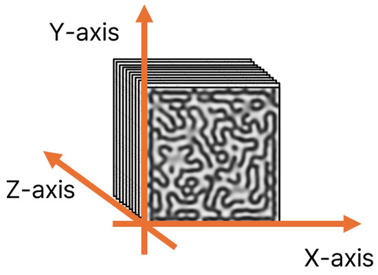
Figure 1.
Definition of the Axes for a Slice Image.
2.1. Multifractal Theory
In this study, the box-counting method is used to calculate the generalised dimensions. In multifractal analysis via the box-counting method, the structure to be analysed is divided into grids, and the grid size is varied from a large size covering the structure to a fine size. Changes in the pixel-existence probability of the structure for each grid can be obtained as the grid size changes, thereby quantifying the overall complexity of the structure. Each divided grid is referred to as a box, and the grid size used for division is termed the box size. The input for the structure to be analysed is typically an image converted to greyscale. When the minimum box size is set to one pixel, the numerical value (pixel value) representing the structure is set to one. The box size is defined as (k is the number of steps), and as the number of steps k increases, the box size is reduced by each time, with the grid divided into equal ratios in both the vertical and horizontal directions. When the box size is ε, the total sum of the pixel values forming the structure in the i-th box is defined as , and the total number of boxes is defined as . Thus, the total sum of the pixel values in the entire input image is . From this, the pixel-existence probability in the i-th box when the box size is ε can be expressed as in Equation (1) [17,18].
Furthermore, via Equation (1), the generalised fractal dimension equation for multifractal analysis is expressed as Equation (2):
where denotes the moment order. By varying the value of the moment order , the high-density ( > 0) and low-density regions ( < 0) in the structure can be highlighted and evaluated [12]. Furthermore, in the plot calculated from , the positive and negative regions of correspond to microscale ( > 0) and macroscale ( < 0) structures, respectively [11]. cannot be defined when because the denominator of becomes zero. From Equation (2), by taking the limit as →1, is defined as in Equation (3):
The multifractal spectrum at = 1 is called the information dimension , and because the numerator in Equation (3) is equivalent to the entropy formula, the limit yields the entropy change (slope) for each box size [17].
Multifractal analysis can calculate the spectrum, and if the calculated spectrum is convex upwards, this indicates the presence of multifractal properties. Here, the expressions for are given by Equations (4) and (5) [19,20,21].
For box size ε, let denote the probability of a pixel being present in the i-th box. The weighted existence probability is then as follows:
At this time, the spectral components and are given by Equations (5) and (6).
Consequently, these are effectively an entropy-related measure that allows us to evaluate whether the information content of the substructures is distributed.
2.2. Proposal 1: Average Method
Extended computational method I is a method of averaging obtained by conducting a multifractal analysis of multiple 2D images. The formula is expressed as Equation (7):
where the j-th slice image is , and the generalised fractal dimension obtained from that image is . W is the thickness in the z-axis direction used, which is the slice thickness.
Similarly, averaging is performed for and, , yielding the expressions given by Equations (8) and (9).
The input data consist of grayscale images, each with pixels. Here, and represent the total number of pixels along the image’s -axis and -axis, respectively. The images are square with . Furthermore, the values of and are given as powers of 2. All the images are sampled using all the pixels at the same pixel interval. Each pixel is assigned an integer value between 0 and 255 (256-level grayscale values). This method applies multifractal analysis directly to the raw data without performing additional processing, such as normalisation.
The extended computation method I is termed the Dq average method and is used to statistically evaluate the generalised fractal dimensions in various multifractal analysis evaluation reports [22].
2.3. Proposal 2: Pixel-Average Method
Extended computation method II is a method to obtain by averaging the pixel values of multiple 2D images by slice thickness and then performing a multifractal analysis. If the slice thickness is W, each XY coordinate is fixed and averaged along the slice direction. The formulas for calculating via extended computation method II are expressed in Equations (10) and (11):
First, let the j-th slice image be , and denote its pixel value as . For the W slice images obtained along the z-axis, averaging each pixel yields Equation (10):
Using the average image , which is the set of pixel values from , we perform a two-dimensional multifractal analysis to obtain the multifractal spectrum from Extended Computation Method II via Equation (11):
where the j-th slice image is , and the pixel value specifying the XY coordinates is .
Similarly, is also calculated via the averaged image, as expressed in Equations (12) and (13).
The input data are identical to those of Proposal 1, consisting of W grayscale images of pixels. Regarding the , plane, as with Proposal 1, all the pixels are used, resulting in equidistant sampling. However, for the z-axis direction, because averaging and integration are performed, the loss of high-resolution information is tolerated.
We call extended computation method II the pixel-averaging method, which performs a pixel-by-pixel averaging process on the pixels at the corresponding positions in each of the multiple 2D images. The generalised fractal dimensions obtained from the averaged image are expected to integrate the structural information between the slice images and capture the complexity of the structure with respect to the slice direction as image shading.
2.4. Proposal 3: PEP Average Method (PEP: Pixel-Existence Probability)
Extended calculation method III calculates the existence probability for each 2D image, averages the existence probability with the slice thickness, and then performs a multifractal analysis to obtain . In this method, the slice thickness W is used to calculate the existence probability for each image. The formula for computation via extended computation method III is shown in Equations (14)–(16).
First, for the j-th slice image , let denote the sum of the pixel values contained within a box for box size , and let denote the sum of the pixel values contained within all boxes. The probability of pixel values existing per box is given by Equation (14).
Next, along the z-axis direction, by averaging the existence probability across all W slices for each box at the same two-dimensional position, we obtain the set of pixel value existence probabilities for box size via Equation (15).
Finally, we vary the box size and calculate the multifractal dimension via Equation (16).
where represents the existence probability at and represents the average existence probability in the slice direction.
Similarly, for , the weighted existence probability is given by Equation (17).
Using this, is given by Equations (18) and (19).
The input data are the same as those of Proposal 1 and Proposal 2, consisting of pixels of grayscale images W. In the plane, an equidistant sampling method using all the pixels is employed. However, unlike Proposals 1 and 2, it calculates the probability distribution by varying the box size for each slice, allowing sampling that accounts for scale differences within each slice. Along the z-axis, probabilities are averaged per box; thus, similar to Proposals 1 and 2, it permits the loss of high-resolution information.
The pixel-existence probability used in the PEP-averaging method is calculated by considering the total number of pixels in each slice and by calculating the pixel-existence probability in one box. Therefore, each box contains the distribution information of the entire slice. These values are averaged for each box at the same location in each slice image, and the resulting average probability distribution is used for multifractal analysis. This is expected to produce a two-dimensional multifractal analysis that reflects the characteristics of the three-dimensional structure because the complexity of the structure in the slice direction is evaluated by considering not only the local structure but also the information of the structure distribution in each slice as a whole.
3. Valuation and Verification of Dispersion in the Slice Direction
In this section, we generate images with different dispersions in the slice direction by controlling the pixel arrangement via Monte Carlo simulations and compare the differences in the generalised fractal dimensions of the three proposed computational extension methods using the obtained simulated images to verify their performance in evaluating dispersion in the slice direction.
3.1. Method of Distributed Image Simulation
In the multifractal analysis, the generalised fractal dimensions were calculated based on the pixel-existence probability of a pixel being present in each box. In other words, by fixing the arrangement of the pixels contained in each box and distributing them randomly in the slice direction, an image with the same pixel arrangement as that observed without regard to the thickness in the slice direction was obtained. This produces a pixel-arrangement pattern with pixels distributed in multiple slices. Simulated images were generated by performing 30 trials for each pattern via the following two steps:
Step 1: Generation of initial images
In this simulation, the number of slices was set to 16. Therefore, for the initial image, 16 images with 128 × 128 pixels as white pixels were prepared, and for each randomly selected slice, black pixels were randomly placed with a target of approximately 40% (6553 pixels) of the 128 × 128 pixels. After placement, the total number of black pixels was checked to confirm that it matched the target value and was determined to be the initial image.
Step 2: Dispersion processing of the pixel arrangement in the slice direction
The initial image obtained in Step 1 was dispersed in the slice direction via two dispersion methods. Dispersion pattern A dispersed the pixels such that the number of pixels in each slice was equal in the direction of the slice. Dispersion pattern B dispersed the pixels nonuniformly in the slice direction such that the number of pixels in each slice varied. These two patterns were used to generate the images.
3.1.1. Pattern A: Simulation with Equal Dispersion
As reported in the literature, when the pixel density and dense pixel area are similar across the entire image, the same results apply to the generalised fractal dimensions shown in the reference literature. In this pattern, the density of each slice was constant to distribute evenly in the slice direction, which can be said to be the same as having multiple images with a constant density. Therefore, if the results are consistent with those of previous studies, the multifractal analysis results for each slice are expected to be the same. Additionally, because the uniform distribution of the pixel density indicates an ideal state with no bias in the pixel distribution, the entropy represented by achieves the highest value within the same pixel density. Thus, the use of these pattern data enables the establishment of a stable standard for generalised fractal dimensions across various methods.
This pattern was applied 30 times, and the simulation data obtained from each trial resulted in data with a constant number of pixels on each slice but with different XY positions for each pixel.
3.1.2. Pattern B: Simulation with Unequal Dispersion
In this pattern, the black pixels in the initial image were arranged such that the 16 images have varying degrees of black pixel density while maintaining their two-dimensional positions. Specifically, 100 pixels were randomly selected from the initial image, and the pixel placement was moved to each slice, with 100 black pixels assigned to each slice image. In this pattern, the number of black pixels placed on each slice was determined as follows. First, for each trial, a random number was selected from the range of 1.5 to 2. For each slice number j along the z-axis, is calculated. This value is used as a weight, and black pixels are distributed to each slice proportionally to the total weight across all slices. This is because if there are slices with no pixels at all, multifractal analysis cannot be performed on those slices. Therefore, the setting is designed to ensure that each slice contains pixels. As a result, these pattern data produce images with nonuniform pixel distributions, and each slice is predicted to have a different local structure. The proposed method is expected to reveal differences in these local structures.
This pattern was implemented 30 times. The simulation data obtained from each trial were random in terms of the number of pixels in each slice, and the XY positions of each pixel were different.
3.2. Results and Methodology Verification
The three computational extension methods proposed in Section 2 were applied to the simulation data generated via Patterns A and B, and the generalised fractal dimensions obtained via each method were calculated. The entire generalised fractal dimension can be evaluated by assessing the distribution of pixel-existence probabilities. Therefore, a comparison was made using the information dimension , which is related to entropy, within the generalised fractal dimensions. In Patterns A and B, the initial images were shared in each trial; therefore, when observed in the slice direction, the pixel arrangement XY was the same. In other words, by examining the amount of change between patterns, the dispersion change in the slice direction can be evaluated. Based on obtained by each computational extension method and each pattern, the change rate is defined as follows:
where indicates each computational expansion method and the applied pattern data.
When the standard error was calculated from obtained by applying each calculation expansion method to 30 trials of Pattern A, it was confirmed that it was less than 0.001 for all calculation expansion methods. This confirms that Pattern A has the same trend as that demonstrated in a previous report [11].
Furthermore, for comparison with , the entropy based on the pixel density for each slice is calculated as an indicator of the bias in the pixel distribution for each trial image in the slice direction, and the entropy change rate is calculated from the variance change for Patterns A and B. The entropy change rate is defined by the following equation:
where is the number of black pixels in each slice, is the pixel density probability for the slice, and is the entropy calculated via Equation (12) for Patterns A and B.
In Figure 2, Equations (10) and (13) are plotted on the vertical axis, and the trial number is plotted on the horizontal axis. The specific values for Figure 2 are attached in Table A1 in Appendix A. Figure 3 shows the relationship between and and dispersion entropy in the slice direction, with entropy S on the horizontal axis and calculated via the two methods on the vertical axis.
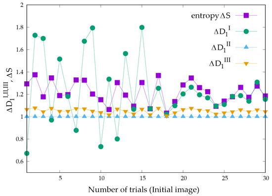
Figure 2.
and entropy for each initial image generated in each trial.
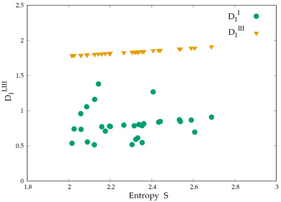
Figure 3.
Relationship between and and dispersion entropy in the slice direction.
Three characteristics were confirmed from the verification results.
Figure 2 shows that all values are 1 when the pixel average method is used. The pixel-averaging method averages pixels in the slice direction while maintaining their positions in a two-dimensional plane. As a result, even if the pixels are distributed uniformly or nonuniformly in the slice direction, the averaged image will be the same as the original image. Therefore, as shown in a previous report [11], had the same value. Thus, the pixel averaging method cannot be used to evaluate three-dimensional pixel dispersion. Therefore, the pixel-averaged method is not used in the following discussion.
Entropy quantifies the unevenness of a distribution and is generally smaller for uneven distributions than for even distributions. Consequently, in the case of even distributions, the entropy is maximised [23]. Therefore, it is theoretically natural that the ratio (change rate) of the simulation image of uniform dispersion pattern A relative to nonuniform dispersion pattern B with pixel distribution bias is greater than or equal to one. However, as shown in Figure 2, with the averaging method, the rate of increase was less than one in five out of 30 trials. This implies that is greater for nonuniform dispersions than for uniform dispersions, resulting in a contradiction. This contradiction suggests that calculated using the average method does not accurately capture the concentration distribution for each slice. Conversely, with the PEP-averaging method, the rate of increase exceeded one for all patterns. This finding is consistent with theory.
As shown in Figure 3, the correlation coefficient between and entropy in the average method was 0.066, indicating no correlation. By contrast, the correlation coefficient between and entropy in the PEP average method was 0.998, indicating a strong correlation. This indicates that the PEP-averaging method can appropriately evaluate the nonuniformity of the concentration distribution in the three-dimensional slice direction and can appropriately evaluate the dispersion of information in the three-dimensional structure.
The above three points demonstrate that the PEP-averaging method is the most effective for evaluating three-dimensional structures.
4. Three-Dimensional Structure Evaluation by Self-Assembly
In this section, we use 3D simulation data obtained via the Gray–Scott model, which produces a self-organising structure, to compare the differences in generalised fractal dimensions obtained from the three proposed computational extension methods, thereby verifying whether it is possible to evaluate the entire 3D structure.
4.1. Theory of the Gray–Scott Model
Fractal structures are characterised by infinite self-similarity when magnified, making it impossible to use conventional evaluation metrics such as length, area, and volume. Consequently, a multifractal analysis was developed as a new metric. This self-similarity is known to be a characteristic of chaos, which is nonperiodic and unpredictable, despite arising from simple rules and orders [24]. Microscopic structures form macroscopic organisations through a simple order process known as self-organisation. Self-organised structures also exhibit self-similarity. The formation process of material microstructures can be simplified into two orders: ‘agglomeration’ and ‘destruction’ or ‘reaction’ and ‘diffusion’, which generate self-organised structures. This self-organising model, which is based on ‘reaction’ and ‘diffusion’, is widely known as a reaction–diffusion system, and a famous mathematical model of the reaction–diffusion system is the Gray–Scott model [25]. The Gray–Scott model is a reproducible model of the phenomenon in which self-organised patterns called dissipative structures are formed by the reaction and diffusion of two types of chemicals. The reaction–diffusion equations of the Gray–Scott model are defined by Equations (24) and (25):
where and are the concentrations of the two chemical substances, and are the reaction–diffusion coefficients, is the supply rate, is the reaction rate constant, and ∆ is the Laplacian operator. The reaction–diffusion equations of the Gray–Scott model are recursive, and by repeating the steps, self-organising patterns are formed from the two equations. By changing the four parameters , , , and , various self-organising patterns can be formed.
Functional composite materials are examples of self-organising systems, similar to Gray–Scott model simulations. The BT/PDVF composite material referenced by the authors possesses a self-organising structure, similar to the Gray–Scott model simulation [26,27]. Furthermore, it has been used to model self-organisation in diverse fields. Examples include research simulating human cell self-organisation via the Gray–Scott model for developing cell-based therapies for tissue repair and research employing the same simulation to generate gold nanostructures through the self-organisation of gold nanoparticles [28,29].
4.2. Generation of Gray–Scott Model Simulation Images
To verify this, we generated three-dimensional self-organising patterns and evaluated three computational extension methods.
First, we prepared a grid space of size 150 × 150 × 150 as the generation size for the self-organising patterns and initialised all grid cells with values of U = 1.0 and V = 0.0. The maximum concentration MAX in each grid cell is one.
Next, as the initial concentration distribution, we randomly explored a 4 × 4 × 4 range area, reduced substance U to 0.25, and increased substance V to 0.5. This process was repeated for approximately 3% of the grid area. Finally, to introduce fluctuations into the initial conditions of the simulation, we randomly added a small amount of noise (0–0.05) to U and V to create an initial image. Figure 4 shows the concentration of the V output as an image. The black rectangles scattered throughout Figure 4 represent the 4 × 4 × 4 regions added as the initial concentration distribution. In addition, noise added as initial image fluctuations can be observed throughout the image.
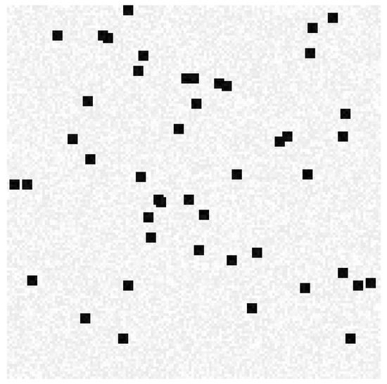
Figure 4.
Initial image generated by the Gray–Scott simulation model.
From this initial state, we performed a simulation by implementing the reaction–diffusion equation of the Gray–Scott model for one million steps. When performing the simulation, the ∆ Laplacian operator in Equations (14) and (15) diffuses the concentrations of substances U and V according to the 3D Laplacian via six neighbours. Laplacian calculations are performed uniformly in three dimensions centred on a single voxel. Therefore, no anisotropy exists in this simulation. During one million steps, when a nonequilibrium steady state appears, the central 128 × 128 × 128 region is trimmed. This is because in the Gray–Scott model, the Laplacian operator cannot be calculated at the edges of the grid space, and the concentrations of substances U and V remain constant. Therefore, trimming was performed to prevent the spatial distribution of concentrations not related to the Gray–Scott simulation parameters from being affected.
This verification took approximately 30 min to complete using a GPU for computation.
In this verification, the parameters for the Gray–Scott model to reach a nonequilibrium steady state were explored via an exhaustive search, and eight pattern datasets were generated. Table 1 lists the parameters and slices of the pattern data obtained as an image. The fractal dimension values shown in Table 1 all become three when the images remain in grayscale. Therefore, the values presented here were obtained by performing fractal analysis on images that were first converted to grayscale and then binarised using a threshold of 128 pixels. The images, which show the concentration of the output V, were used to evaluate the extended-calculation method. Among these patterns, those with connected black pixels (concentration) are called network patterns, and those with black pixels scattered in spheres are called spot patterns.

Table 1.
Gray–Scott model parameters that produce a nonequilibrium steady state.
4.3. Results and Discussion
In this section, we compare the differences in the generalised fractal dimensions of the three proposed computational extension methods via the pattern data obtained from the eight parameters. Because each pattern data point is a three-dimensional cube, we performed slicing in three directions to obtain generalised fractal dimensions. Figure 5 shows plots of the concentration of each pattern and the values of calculated via each computational extension method. The x-, y-, and z-axes correspond to the coordinate axes shown in Section 2. The plot of in Figure 5 shows the standard error resulting from the averaging process. Since and produce unique values, they do not have a standard error. In addition, it was verified that fractal properties were consistently observed across all patterns and analysis methods, as described in Appendix B.
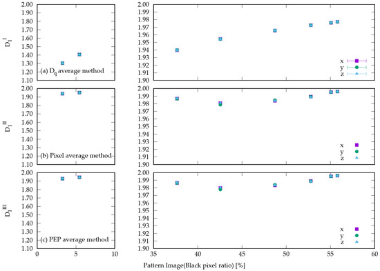
Figure 5.
Relationship between the concentration and for each pattern of data grouped via the extended calculation method.
The results of the comparison in Figure 5 revealed three characteristics.
The generalised fractal dimensions of each pattern data from the three directions confirmed that remained almost unchanged regardless of the direction of the analysis. The standard error of for each direction was less than 0.001 for all calculation extension methods and patterns. This is because the Gray–Scott model used for pattern formation utilises the Laplacian of six neighbours, suggesting that the concentration structure grows similarly in all three directions. Therefore, each calculation extension method can be applied to isotropic three-dimensional structures.
Using the averaging method, we confirmed that increased as the concentration increased from 30% to 60%. This is consistent with the theoretical property that, as reported in previous studies [11], the information dimension approaches the maximum value of two exponentially as the concentration increases, based on concentration-dependent generalised fractal dimensions. By contrast, in the PEP- and pixel-average method, for low-concentration Patterns 7 and 8, the black pixels are scattered mainly as isolated spots and have little spatial connectivity. From this structure, as the concentration increased with changes in the parameters, the number of spots increased, and the value of also increased with increasing concentration (Pattern 6). After the number of spots reached the limit, further increases in concentration began to create connections between the spots. The spots connect with each other to form larger concentration clusters, and , which reflects dispersion, decreases (Pattern 5). As the concentration continued to increase, all the spots were connected, and the concentration pattern began to adopt a network pattern, eventually growing into a surface structure. The parameters of the grayscale model used in this study, which are in a nonequilibrium steady state, represent the stage of concentration structure growth.
In Patterns 7 and 8, which had low concentrations, the average method yielded lower values than in the other methods. This is because in the calculation of , when an equation similar to entropy as the numerator is used, the greater the number of probabilities that are calculated, the higher the value obtained. In the PEP and pixel-averaging methods, the values of are considered higher because they directly affect the probability distribution. In other words, they calculated the generalised fractal dimensions by considering the distribution in the slice direction.
From the above, it was confirmed that in the average method, the generalised fractal dimensions change with concentration and do not reflect three-dimensional structural changes. Conversely, in the PEP-averaging method and pixel-averaging method, even when the concentration continues to increase, the generalised fractal dimensions fluctuate owing to the three-dimensional concentration structure, confirming that they can reflect the three-dimensional structural changes within the pattern.
However, this method is an extension of the two-dimensional multifractal analysis method. As in the two-dimensional multifractal analysis method, pixel changes and missing values affect the values and cannot be analysed.
5. Conclusions
In this study, we propose three extended-calculation methods that summarise the spread of three-dimensional structures onto a two-dimensional plane based on the generalised dimensional formula of two-dimensional multifractal analysis for three-dimensional structures. The effectiveness of each extended-calculation method was confirmed via Monte Carlo and Gray–Scott simulations. The results show that the PEP averaging method can evaluate structural dispersion information in the slice (3D) direction and that the entropies and in the slice direction are strongly correlated. Furthermore, it was confirmed that structures that cannot be evaluated via conventional 2D images alone, owing to the saturation of values, can be more accurately evaluated via the proposed method.
Therefore, the two-dimensional multifractal analysis method for three-dimensional structures proposed in this paper is expected to contribute to the advancement of morphometrics by assisting in the understanding of three-dimensional structures from two-dimensional multifractal analysis results of surface structures.
Author Contributions
Conceptualization, methodology, software, validation, formal analysis, investigation, resources, and data curation, A.T. and Y.S.; writing—original draft preparation, A.T.; writing—review and editing, visualization, supervision, project administration, and funding acquisition, Y.S. All authors have read and agreed to the published version of the manuscript.
Funding
This work was supported by the 2025 TOKYO CITY UNIVERSITY Priority Promotion Early Career Scientists Research grant.
Data Availability Statement
The original contributions presented in this study are included in the article, and further inquiries can be directed to the corresponding author.
Conflicts of Interest
The authors declare no conflicts of interest.
Appendix A
Table A1.
Values of and entropy ∆S for each initial image generated in each trial.
Table A1.
Values of and entropy ∆S for each initial image generated in each trial.
| Number of Trials | Entropy ∆S | |||
|---|---|---|---|---|
| 1 | 1.2935960 | 0.6726074 | 0.9999534 | 1.0653261 |
| 2 | 1.3752910 | 1.7281945 | 0.9999534 | 1.0791908 |
| 3 | 1.1777972 | 1.7000611 | 0.9999534 | 1.0448574 |
| 4 | 1.3469162 | 0.9697403 | 0.9999534 | 1.0758888 |
| 5 | 1.1887294 | 1.5154851 | 0.9999534 | 1.0483877 |
| 6 | 1.1972921 | 1.1820644 | 0.9999534 | 1.0488341 |
| 7 | 1.3286980 | 0.8784778 | 0.9999534 | 1.0726144 |
| 8 | 1.3266124 | 1.6755119 | 0.9999534 | 1.0709015 |
| 9 | 1.2025691 | 1.7942907 | 0.9999534 | 1.0498063 |
| 10 | 1.1520390 | 0.7323597 | 0.9999534 | 1.0375790 |
| 11 | 1.0635399 | 1.3355127 | 0.9999534 | 1.0176194 |
| 12 | 1.3047466 | 0.7999125 | 0.9999534 | 1.0691615 |
| 13 | 1.1934109 | 1.5645343 | 0.9999534 | 1.0483230 |
| 14 | 1.0943972 | 1.0658812 | 0.9999534 | 1.0246358 |
| 15 | 1.3055950 | 1.7990874 | 0.9999534 | 1.0678811 |
| 16 | 1.0703669 | 1.0709745 | 0.9999534 | 1.0180825 |
| 17 | 1.3685292 | 1.2540443 | 0.9999534 | 1.0762876 |
| 18 | 1.0314567 | 1.0221169 | 0.9999534 | 1.0076374 |
| 19 | 1.1356704 | 1.0978999 | 0.9999534 | 1.0350160 |
| 20 | 1.2839586 | 1.2035429 | 0.9999534 | 1.0640828 |
| 21 | 1.3461463 | 1.2642253 | 0.9999534 | 1.0758348 |
| 22 | 1.2597768 | 1.1959571 | 0.9999534 | 1.0583868 |
| 23 | 1.2236903 | 1.1685399 | 0.9999534 | 1.0536964 |
| 24 | 1.0924876 | 1.0954151 | 0.9999534 | 1.0238992 |
| 25 | 1.1392720 | 1.1093918 | 0.9999534 | 1.0348228 |
| 26 | 1.1781465 | 1.1810969 | 0.9999534 | 1.0445545 |
| 27 | 1.2619710 | 1.1887206 | 0.9999534 | 1.0623428 |
| 28 | 1.1739030 | 1.1390590 | 0.9999534 | 1.0443692 |
| 29 | 1.2739621 | 1.3090071 | 0.9999534 | 1.0611155 |
| 30 | 1.1855635 | 1.1555629 | 0.9999534 | 1.0457690 |
Appendix B
Figure A1 shows the vs. graph. It can be confirmed that the vs. graph is convex upwards in all patterns under extended computation methods 1, 2 and 3, verifying that fractal properties can be evaluated. The plot of and in Figure 5 shows the standard error resulting from the averaging process. Since , , and produce unique values, they do not have a standard error.


Figure A1.
vs. for each pattern data point grouped via the extended-calculation method.
References
- Vaz, C.; Pascoal, R.; Sebastião, H. Price appreciation and roughness duality in bitcoin: A multifractal analysis. Mathematics 2021, 9, 2088. [Google Scholar] [CrossRef]
- Lopes, R.; Betrouni, N. Fractal and multifractal analysis: A review. Med. Image Anal. 2009, 13, 634–649. [Google Scholar] [CrossRef]
- Jiang, Z.-Q.; Xie, W.-J.; Zhou, W.-X.; Sornette, D. Multifractal analysis of financial markets: A review. Rep. Prog. Phys. 2019, 82, 125901. [Google Scholar] [CrossRef] [PubMed]
- Hirabayashi, T.; Ito, K.; Yoshii, T. Multifractal analysis of earthquakes. Pure Appl. Geophys. 1992, 138, 591–610. [Google Scholar] [CrossRef]
- Ebrahimkhanlou, A.; Farhidzadeh, A.; Salamone, S. Multifractal analysis of crack patterns in reinforced concrete shear walls. Struct. Health Monit. 2016, 15, 81–92. [Google Scholar] [CrossRef]
- López-Lambraño, A.A.; Fuentes, C.; Serpa-Usta, Y.; Tejada, G.; López-Ramos, A. Multifractal Measures and Singularity Analysis of Rainfall Time Series in the Semi-Arid Central Mexican Plateau. Atmosphere 2025, 16, 639. [Google Scholar] [CrossRef]
- Salat, H.; Murcio, R.; Arcaute, E. Multifractal Methodology. Phys. A Stat. Mech. Appl. 2017, 473, 467–487. [Google Scholar] [CrossRef]
- Wu, J.; Jin, X.; Mi, S.; Tang, J. An Effective Method to Compute the Box-Counting Dimension Based on the Mathematical Definition and Intervals. Results Eng. 2020, 6, 100106. [Google Scholar] [CrossRef]
- Rajković, N.; Krstonošić, B.; Milošević, N. Box-Counting Method of 2D Neuronal Image: Method Modification and Quantitative Analysis Demonstrated on Images from the Monkey and Human Brain. Comput. Math. Methods Med. 2017, 2017, 8967902. [Google Scholar] [CrossRef]
- Liu, S.; Chen, Y. A Three-Dimensional Box-Counting Method to Study the Fractal Characteristics of Urban Areas in Shenyang, Northeast China. Buildings 2022, 12, 299. [Google Scholar] [CrossRef]
- Sato, Y.; Munakata, F. Morphological characteristics of self-assembled aggregate textures using multifractal analysis: Interpretation of multifractal τ(q) using simulations. Phys. A Stat. Mech. Appl. 2022, 603, 127771. [Google Scholar] [CrossRef]
- Munakata, F.; Ogiya, T.; Sato, Y. Thermal conductivities and complex network properties of fractal self-assembled/self-organized texture in binary composite materials. Appl. Phys. A 2024, 130, 522. [Google Scholar] [CrossRef]
- Breki, C.-M.; Dimitrakopoulou-Strauss, A.; Hassel, J.; Theoharis, T.; Sachpekidis, C.; Pan, L.; Provata, A. Fractal and multifractal analysis of PET/CT images of metastatic melanoma before and after treatment with ipilimumab. EJNMMI Res. 2016, 6, 61. [Google Scholar] [CrossRef] [PubMed]
- Horstmann, H.; Körber, C.; Sätzler, K.; Aydin, D.; Kuner, T. Serial section scanning electron microscopy (S3EM) on silicon wafers for ultra-structural volume imaging of cells and tissues. PLoS ONE 2012, 7, e35172. [Google Scholar] [CrossRef]
- Phaneuf, M.W. FIB for Materials Science Applications—A Review; Springer: Boston, MA, USA, 2005; Volume 30, pp. 277–288. ISBN 9780387231167. [Google Scholar]
- Fiske, L.D.; Aalders, M.C.G.; Almasian, M.; van Leeuwen, T.G.; Katsaggelos, A.K.; Cossairt, O.; Faber, D.J. Bayesian analysis of depth resolved OCT attenuation coefficients. Sci. Rep. 2021, 11, 2263. [Google Scholar] [CrossRef]
- Halsey, T.C.; Jensen, M.H.; Kadanoff, L.P.; Procaccia, I.; Shraiman, B.I. Fractal measures and their singularities: The characterization of strange sets. Phys. Rev. A Gen. Phys. 1986, 33, 1141–1151. [Google Scholar] [CrossRef]
- Kermouni Serradj, N.; Messadi, M.; Lazzouni, S. Classification of mammographic ROI for microcalcification detection using multifractal approach. J. Digit. Imaging 2022, 35, 1544–1559. [Google Scholar] [CrossRef]
- Yadav, R.P.; Dwivedi, S.; Mittal, A.K.; Kumar, M.; Pander, A.C. Fractal and multifractal analysis of LiF thin film surface. Appl. Surf. Sci. 2012, 261, 547–553. [Google Scholar] [CrossRef]
- Xiong, G.; Yu, W.; Xia, W.; Zhang, S. Multifractal signal reconstruction based on singularity power spectrum. Chaos Solitons Fractals 2016, 91, 25–32. [Google Scholar] [CrossRef]
- Chen, Y.; Wang, J. Multifractal characterization of urban form and growth: The case of Beijing Environ. Plan. B Plan. Des. 2013, 40, 884–904. [Google Scholar] [CrossRef]
- Wang, F.; Liao, D.W.; Li, J.W.; Liao, G.P. Two-dimensional multifractal detrended fluctuation analysis for plant identification. Plant Methods 2015, 11, 12. [Google Scholar] [CrossRef]
- Shannon, C.E. A mathematical theory of communication. Bell Syst. Tech. J. 1948, 27, 379–423. [Google Scholar] [CrossRef]
- Boeing, G. Visual analysis of nonlinear dynamical systems: Chaos, fractals, self-similarity and the limits of prediction. Systems 2016, 4, 37. [Google Scholar] [CrossRef]
- Gray, P.; Scott, S.K. Autocatalytic reactions in the isothermal, continuous stirred tank reactor. Chem. Eng. Sci. 1983, 38, 29–43. [Google Scholar] [CrossRef]
- Zhang, Z.X.; Jin, Z.; Lu, B.; Xin, Z.X.; Kang, C.K.; Kim, J.K. Effect of Flame Retardants on Mechanical Properties, Flammability and Foamability of PP/Wood–Fiber Composites. Compos. Part B Eng. 2012, 43, 150–158. [Google Scholar] [CrossRef]
- Lee, C.H.; Salit, M.S.; Hassan, M.R. A Review of the Flammability Factors of Kenaf and Allied Fibre Reinforced Polymer Composites. Adv. Mater. Sci. Eng. 2014, 2014, 514036. [Google Scholar] [CrossRef]
- Garfinkel, A.; Tintut, Y.; Petrasek, D.; Boström, K.; Demer, L.L. Pattern Formation by Vascular Mesenchymal Cells. Proc. Natl. Acad. Sci. USA 2004, 101, 9247–9250. [Google Scholar] [CrossRef]
- Chen, T.-H.; Hsu, J.J.; Zhao, X.; Guo, C.; Wong, M.N.; Huang, Y.; Li, Z.; Garfinkel, A.; Ho, C.-M.; Tintut, Y.; et al. Left-Right Symmetry Breaking in Tissue Morphogenesis via Cytoskeletal Mechanics. Circ. Res. 2012, 110, 551–559. [Google Scholar] [CrossRef]


Disclaimer/Publisher’s Note: The statements, opinions and data contained in all publications are solely those of the individual author(s) and contributor(s) and not of MDPI and/or the editor(s). MDPI and/or the editor(s) disclaim responsibility for any injury to people or property resulting from any ideas, methods, instructions or products referred to in the content. |
© 2025 by the authors. Licensee MDPI, Basel, Switzerland. This article is an open access article distributed under the terms and conditions of the Creative Commons Attribution (CC BY) license (https://creativecommons.org/licenses/by/4.0/).