Article

Adaptive Tree-Structured MTS with Multi-Class Mahalanobis Space for High-Performance Multi-Class Classification

1
College of Modern Science and Technology, China Jiliang University, Jinhua 322000, China
2
School of Economics and Management, China Jiliang University, Hangzhou 310018, China
*
Author to whom correspondence should be addressed.
Mathematics 2025, 13(19), 3233; https://doi.org/10.3390/math13193233
Submission received: 4 September 2025 / Revised: 7 October 2025 / Accepted: 8 October 2025 / Published: 9 October 2025

Abstract

The traditional Mahalanobis–Taguchi System (MTS) employs two main strategies for multi-class classification: the partial binary tree MTS (PBT-MTS) and the multi-tree MTS (MT-MTS). The PBT-MTS relies on a fixed binary tree structure, resulting in limited model flexibility, while the MT-MTS suffers from its dependence on pre-defined category partitioning. Both methods exhibit constraints in adaptability and classification efficiency within complex data environments. To overcome these limitations, this paper proposes an innovative Adaptive Tree-structured Mahalanobis–Taguchi System (ATMTS). Its core breakthrough lies in the ability to autonomously construct an optimal multi-layer classification tree structure. Unlike conventional PBT-MTS, which establishes a Mahalanobis Space (MS) containing only a single category per node, ATMTS dynamically generates the MS that incorporates multiple categories, substantially enhancing discriminative power and structural adaptability. Furthermore, compared to MT-MTS, which depends on prior label information, ATMTS operates without predefined categorical assumptions, uncovering discriminative relationships solely through data-driven learning. This enables broader applicability and stronger generalization capability. By introducing a unified multi-objective joint optimization model, our method simultaneously optimizes structure construction, feature selection, and threshold determination, effectively overcoming the drawbacks of conventional phased optimization approaches. Experimental results demonstrate that ATMTS outperforms PBT-MTS, MT-MTS, and other mainstream classification methods across multiple benchmark datasets, achieving significant improvements in the accuracy and robustness of multi-class classification tasks.

1. Introduction

Data classification serves as a fundamental technique in data mining for extracting valuable information. While binary classification is well-studied, real-world problems often involve multiple categories, making multi-class classification a more prevalent and challenging the focus of recent research. Numerous well-established machine learning techniques, such as support vector machine (SVM), k-nearest neighbor (KNN), artificial neural networks (ANNs), and random forest (RF), have been developed and extensively applied across diverse domains. These applications include fault diagnosis [1,2,3], air pollution prediction [4], disease diagnosis [5], defect detection [6], and financial risk prediction [7].
Originating from quality engineering, the Mahalanobis–Taguchi System (MTS) has emerged as a robust pattern recognition technique. It distinguishes itself from the aforementioned algorithms by its distinct advantages: it requires no assumptions regarding data distribution, demonstrates high efficiency in feature reduction, and is notably straightforward to implement [8]. Furthermore, MTS has also been demonstrated to be a promising classifier for handling imbalanced data [9]. Owing to these strengths, MTS has been widely adopted in various fields, including product quality inspection [10], hotel recommendation [11], multivariate process control [12], and health performance assessment [13]. These applications have consistently demonstrated the MTS’s commendable classification performance.
Initially developed for binary classification, the conventional MTS faces limitations when applied to real-world scenarios where multi-class classification is more prevalent. To leverage the advantages of MTS in multi-class problems, scholars have proposed two primary approaches. The first type is establishing a Mahalanobis space (MS) for each individual category and calculating the Mahalanobis distance (MD) of unknown samples relative to each MS. Classification is then determined by selecting the category corresponding to the shortest MD [14]. However, scholars had stated that this method cannot be used to identify abnormal samples that do not belong to any predefined category. To address this shortcoming, an enhanced approach is developed wherein a specific threshold is established for each category’s MS. The MD of a sample is compared against these thresholds, enabling not only multi-class classification but also the detection of abnormal samples, thereby improving overall classification accuracy [15]. Consider a classification problem with k classes. This approach requires constructing k individual binary MTS classifiers during the training phase. Throughout the testing stage, the MD must be computed k times for each sample. As the number of classes and the sample size grow, this process imposes a substantial computational burden and severely compromises classification efficiency.
Consequently, researchers have developed a second category of solutions by decomposing multi-class problems into multiple binary classification tasks, thereby extending the applicability of MTS. Representative algorithms in this category include the directed acyclic graph MTS (DAG-MTS) [16], PBT-MTS [17], and multi-tree MTS (MT-MTS) [18]. During the testing stage, the DAG-MTS algorithm requires only k 1 binary classifiers to determine the class of a sample. However, the training phase necessitates the construction of k ( k 1 ) / 2 binary classifiers, resulting in substantial computational overhead and limiting its practical adoption [19]. Binary tree structures offer an alternative due to their relatively low complexity and efficient training. These can be categorized into the partial binary tree (PBT) and complete binary tree (CBT). In conventional MTS practice, where each binary classifier establishes only one MS using samples from a single class, the method is typically integrated with a PBT architecture for multi-class classification [17]. However, the CBT is often a superior classifier architecture owing to its shallower depth and reduced classification time. To leverage these advantages, some researchers have integrated MTS with a multi-tree (MT) structure, for instance in fault type and severity diagnosis of rolling bearings [18]. The MT structure represents an intermediate form between the PBT and CBT, achieving relatively shallow tree depth and moderately improved classification efficiency. Nevertheless, a major limitation of MT is its dependence on predefined hierarchical information of the data, which restricts its applicability to specific scenarios and limits generalizability.
In response to the aforementioned limitations, this study proposes the Adaptive Tree-structured Mahalanobis–Taguchi System (ATMTS) for multi-class classification. The approach constructs an adaptive tree-structured framework through a joint optimization model that simultaneously optimizes the construction of the MS, feature variable selection, and threshold determination.
Section 2 introduces the foundational methodologies, including the MTS, tree-structured MTS multi-class classification method, and the hybrid multi-objective particle swarm optimization (HMOPSO) algorithm. Section 3 provides a detailed exposition of the proposed ATMTS. Experimental results and comparative analyses are presented in Section 4. Finally, Section 5 concludes the paper and suggests potential avenues for future research.

2. Relevant Theories

2.1. Mahalanobis–Taguchi System

In the early 1990s, Japanese quality engineer Genichi Taguchi introduced the MTS. The MTS is built upon four core theoretical components: the MD, orthogonal experiment design, the signal-to-noise ratio (SNR), and the threshold [20,21,22]. Specifically, the MD is a statistical measure used to quantify the similarity between samples, accounting for correlations among variables while remaining scale-invariant. Orthogonal experimental design is employed for feature selection; it utilizes orthogonal arrays to systematically organize trials, thereby identifying effective feature combinations with minimal experimental effort. The SNR, literally referring to the ratio of signal to noise, serves in MTS as an indicator of system performance, higher SNR values correspond to better discriminatory power of the system. Finally, the threshold acts as a decision boundary that separates normal samples from abnormal ones. Its appropriate setting is critical to the accuracy of the classification process.
Assuming a sample size of n with p feature variables. The dataset can be represented as an n × p matrix:
x 11 x 1 p x n 1 x n p
where i = 1 , 2 , , n and k = 1 , 2 , , p .
The standard implementation procedure of the MTS is outlined as follows:
Step 1 
Construction of the MS
The MS is constructed using normal samples, which are typically defined by domain experts based on prior knowledge or diagnostic criteria and represent the benchmark healthy or standard operating condition. Suppose the first m samples are designated as normal. The MD of the i -th normal sample is computed as:
M D i = 1 m Z i T C 1 Z i
where Z i T = z i 1 , z i 2 , z i p is the standardized vector of the i -th sample, z i k = x i k x k ¯ s k is the standardized value, x k ¯ = i = 1 n x i k n is the mean of the k -th feature, s k = 1 n 1 i = 1 n x i k x k ¯ 2 is the standard deviation of the k -th feature, and C = 1 m 1 i = 1 m Z i Z i T is the correlation coefficient matrix estimated from the normal samples.
Step 2 
Validation of the MS
The abnormal samples are first normalized using the mean and standard deviation derived from the normal samples. The Mahalanobis Distances (MDs) of these abnormal samples are then computed based on the constructed MS. Finally, the MDs of the abnormal samples are compared against those of the normal samples. The MS is considered valid if the MDs of the abnormal samples are significantly larger than those of the normal samples.
Step 3 
Feature selection and MS optimization
An appropriate two-level orthogonal array is first selected based on the number of features [23]. For instance, in the case of the commonly used iris dataset, which contains four features, an L 8 2 7 orthogonal array can be employed. This is a normalized experimental design table, in which the number 7 indicates the maximum number of factors that can be assigned, 2 represents the number of levels per factor, and 8 specifies the number of experimental runs required. In this design, Level-1 indicates the inclusion of a feature, while Level-2 denotes its exclusion. For each experimental combination defined by the orthogonal array, the MDs of the abnormal samples are computed. The signal-to-noise ratio (SNR) is then utilized to evaluate the effectiveness of each feature subset. Since larger MD values are more indicative of abnormal samples, the larger-the-better SNR (SNRLB) is employed in the MTS to identify the most discriminative feature subset.
Assuming a two-level orthogonal array L n 2 q is used, the SNRLB for the i th experiment is as follows:
η i = 10 lg 1 n m j = m + 1 n 1 M D i j
where j is the number of abnormal samples, and M D i j is the MD of j j = m + 1 , m + 2 , n th abnormal sample in the i -th experiment regarding the MS. For each feature variable, the gain value of SNRLB was calculated. This value is obtained by subtracting the mean SNRLB value from experiments that did not use the feature variable from the mean SNRLB value of experiments that did use the feature variable. If the SNRLB’s gain value is positive, the feature variable is retained; if not, it is discarded.
The selected features are then used to reconstruct the MS. Within this optimized MS, the MDs are calculated for both normal and abnormal samples. This optimized MS enhances the discrimination between normal and abnormal samples by making their MD distributions more distinct.
Step 4 
Calculate threshold value
In the conventional MTS, Genichi Taguchi introduced the quadratic loss function (QLF) to establish the threshold value [24]. The Mahalanobis distances of the samples to be classified are then computed within the optimized Mahalanobis Space (MS). A sample is classified as normal if its MD is less than or equal to the threshold; otherwise, it is classified as abnormal.

2.2. Tree-Structured MTS Multi-Class Classification Method

While the standard MTS is fundamentally designed for binary classification, its integration with tree-structured frameworks enables effective multi-class classification. This section provides a systematic overview and comparative analysis of two prominent tree-based MTS extensions: the PBT-MTS, the MT-MTS and the DAG-MTS, highlighting their structural characteristics, operational mechanisms, and applicability domains.
The PBT-MTS employs a one-versus-all strategy, sequentially separating one category from the remaining classes at each node. As illustrated in Figure 1, beginning from the root node, one class is treated as the normal group for MS construction, while samples from all other categories are collectively regarded as abnormal. An MTS binary classifier is trained at each internal node, including optimization of feature variables and threshold determination via quadratic loss function (QLF) or similar criteria. This iterative partitioning continues until all classes are discerned. Although conceptually straightforward, PBT-MTS requires training k 1 classifiers for k classes, which can become computationally expensive for large-scale or high-dimensional datasets [17].
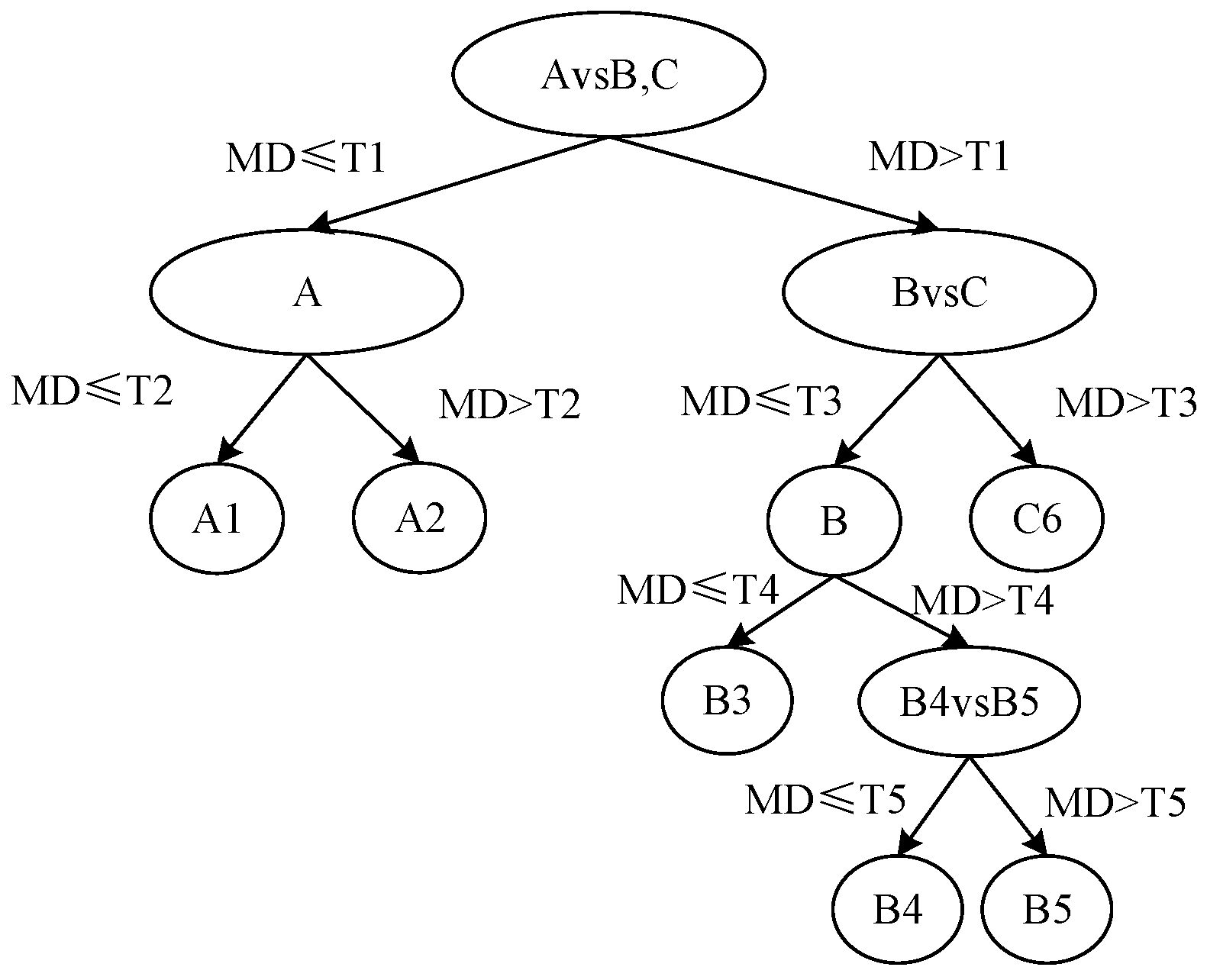
In contrast, the MT-MTS is particularly suitable for datasets exhibiting inherent hierarchical structure, such as fault diagnostics with multi-level severity or biological taxonomies. As depicted in Figure 2, the MT-MTS operates on multiple classification levels. The first level distinguishes coarse categories (e.g., A, B, C, D), while subsequent levels perform finer-grained classification within each parent category (e.g., A1, A2 under A). Each non-leaf node functions as an MTS binary classifier. This structure allows certain branching paths to be processed concurrently, improving computational efficiency compared to the strictly sequential PBT-MTS [18]. However, its performance highly depends on predefined hierarchical knowledge, which may not be available in all applications.
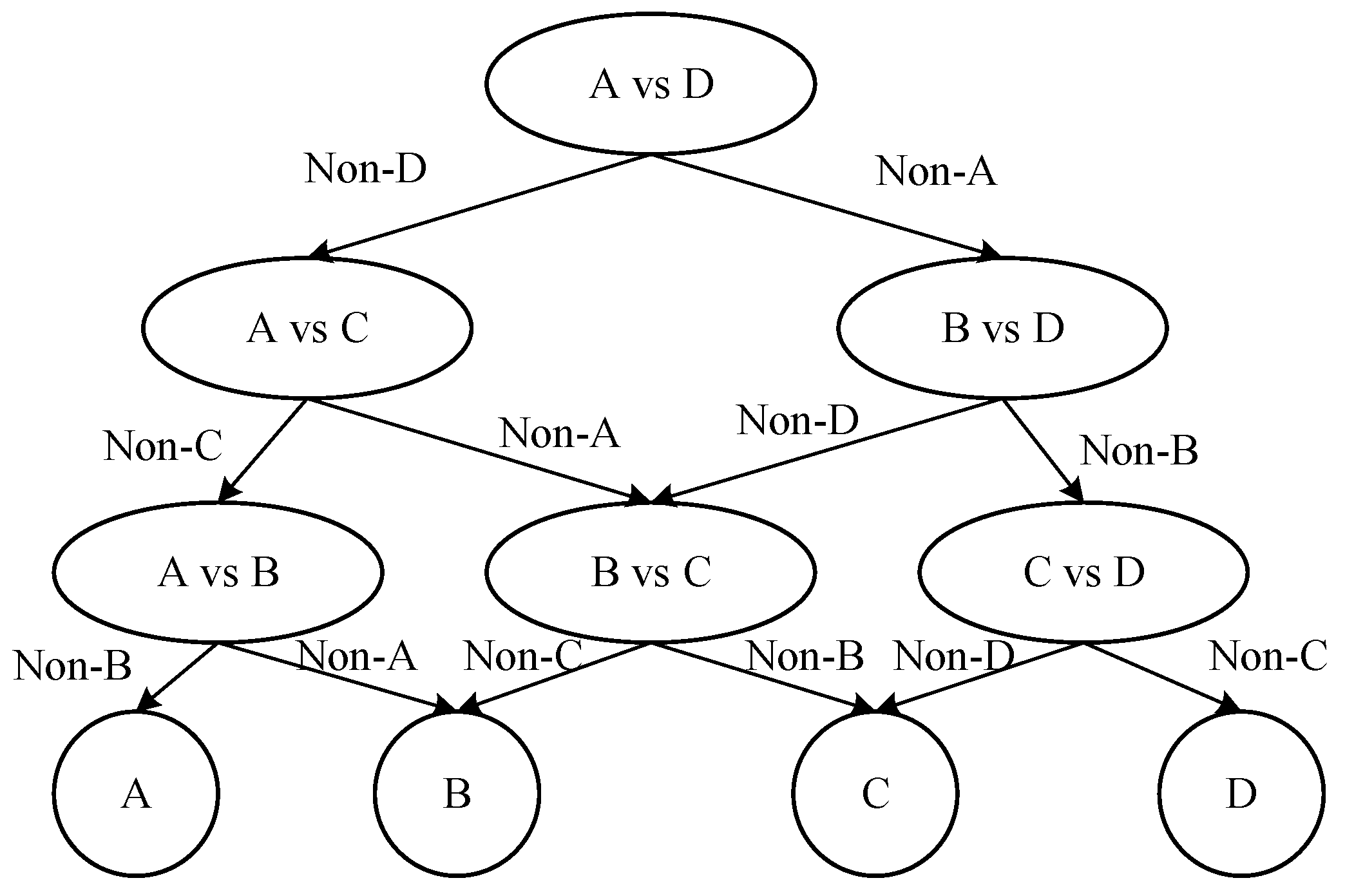
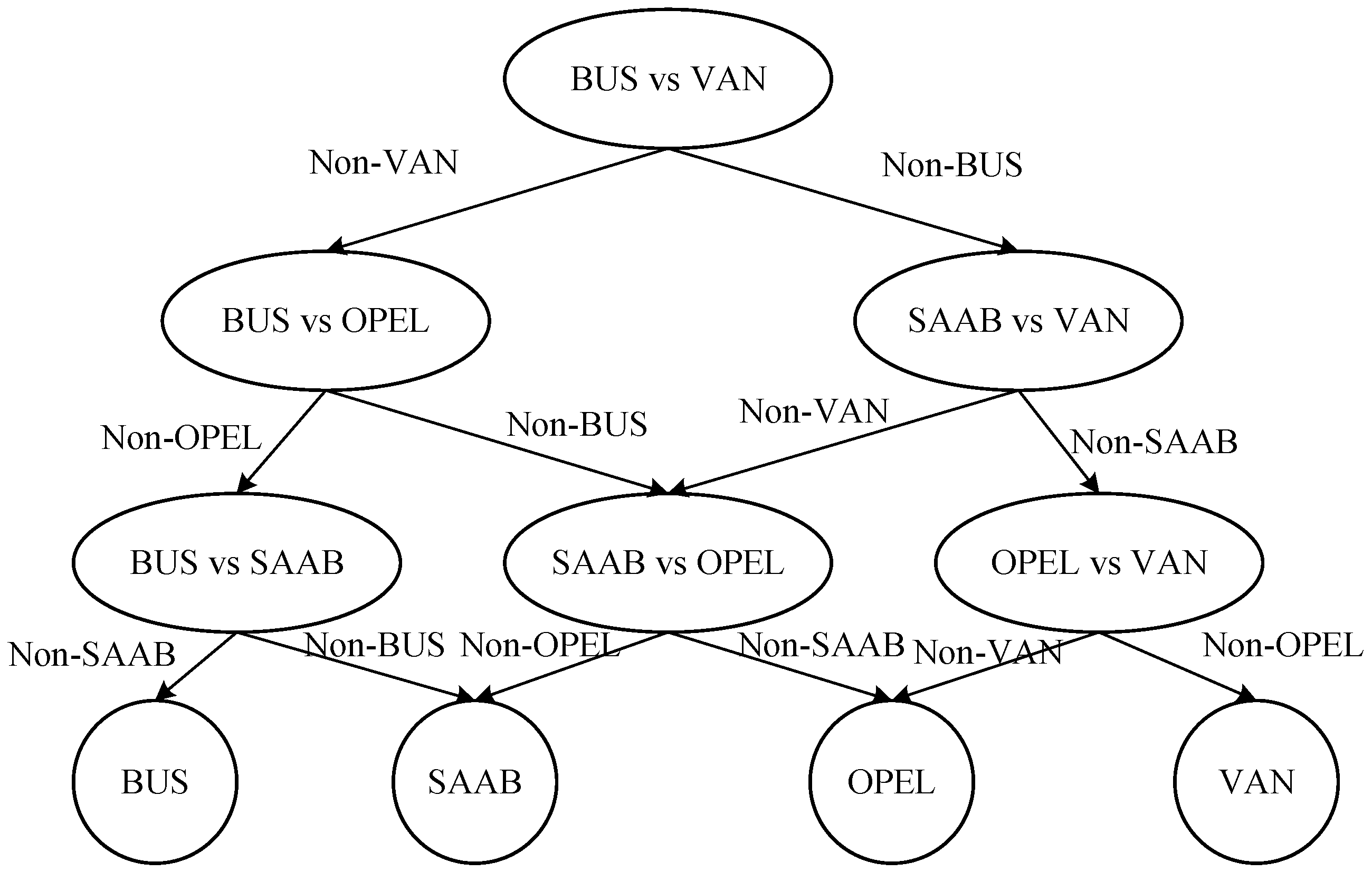
In the DAG-MTS method, an MTS classifier is constructed at each node (except the leaf nodes) to address the multi-class classification problem, as illustrated in Figure 3. During the classification process, one class is designated as the normal sample and another as the abnormal sample to build the MTS. For a test sample, if the MD exceeds the threshold, it is concluded that the sample does not belong to the normal class; if MD less than or equal to the threshold, it is concluded that the sample does not belong to the abnormal class. This process continues iteratively until a definitive “either A or B” binary decision is reached.

2.3. Hybrid Multi-Objective Particle Swarm Optimization Algorithm

This paper proposes a multi-objective joint optimization model involving both discrete and continuous decision variables. To effectively address this hybrid optimization challenge, a hybrid multi-objective particle swarm optimization (HMOPSO) algorithm is adopted. This hybrid approach maintains the parameter efficiency and implementation simplicity of PSO-based methods while enabling simultaneous optimization of conflicting objectives in complex search spaces. Comparative studies have shown that HMOPSO achieves better convergence characteristics and computational efficiency than genetic algorithm variants for medium-scale hybrid optimization problems [25,26], making it particularly suitable for the MTS optimization task addressed in this study. As described by Algorithm 1, the HMOPSO algorithm has the following key steps.
Algorithm 1. The HMOPSO algorithm
Input:
N: Number of particles
M: Number of objective functions
maxIter: Maximum iterations
bounds_cont: Continuous variable boundaries [lb1, ub1], [lb2, ub2], …, [lbₙ, ubₙ]
bounds_disc: Discrete variable boundaries [min1, max1], [min2, max2], …, [minₘ, maxₘ]
Output:
gbest: Global best solution (non-dominated solutions in Pareto front)

1: // Initialization phase
2: Initialize particle population population
3: For i = 1 to N do:
4:    Initialize continuous position x_cont
5:    Initialize continuous velocity v_cont
6:    Initialize discrete position x_disc
7:    Initialize discrete velocity v_disc
8:    Calculate fitness fitness
9:    Set personal best pbest
10:     Set personal best fitness pbest_fitness
11:     Add particle to population
12: End For

13: // Initialize global best
14: gbest ← select non-dominated solutions from population
15: gbest_fitness ← corresponding fitness values

16: // Main loop
17: For iter = 1 to maxIter do:
18:    For each particle in population do:
19:      // Update continuous variables
20:      Generate random vectors r1, r2 ∈ [0, 1]^n
21:      Update continuous velocity:
22:         v_cont ← w × v_cont + c1 × r1 × (pbest_cont − x_cont) + c2 × r2 × (gbest_cont − x_cont)
23:      Update continuous position:
24:         x_cont ← x_cont + v_cont
25:      Apply boundary constraints to ensure x_cont remains within bounds_cont
26:
27:      // Update discrete variables
28:      Generate random vectors r1_disc, r2_disc ∈ [0, 1]^m
29:      Update discrete velocity:
30:         v_disc ← c1 × r1_disc × (pbest_disc − x_disc) + c2 × r2_disc × (gbest_disc − x_disc)
31:      Convert velocity to probability:
32:         prob ← sigmoid(v_disc) = 1/(1 + exp(-v_disc))
33:      For each discrete variable j do:
34:         If rand() < prob[j] then:
35:           x_disc[j] ← randomly flip within bounds_disc[j]
36:         End If
37:
38:      // Evaluate new position
39:      new_fitness ← evaluate(x_cont, x_disc)
40:
41:      // Update personal best
42:      If new_fitness dominates pbest_fitness then:
43:         pbest ← (x_cont, x_disc)
44:         pbest_fitness ← new_fitness
45:      End If
46:    End For
47:
48:    // Update global best
49:    Update gbest by selecting non-dominated solutions from all particles’ pbest
50:
51:    // Optional: Apply mutation operation to maintain diversity
52:    Mutate particles with a certain probability
53: End For
54: Return gbest// Return the found Pareto optimal solution set
A practical analogy for HMOPSO’s mixed-variable optimization is the design of a marketing strategy. This process involves optimizing both discrete variables, such as the primary advertising channel, and continuous variables, such as the precise budget allocation. HMOPSO functions like a data-driven analyst, evaluating candidate strategies, or particles, against multiple objectives like maximizing customer reach and minimizing cost. It iteratively refines these strategies by learning from past performance: probabilistically favoring discrete choices that prove effective and making fine-grained adjustments to continuous parameters. This approach efficiently converges on a set of optimal trade-off solutions without the need for exhaustive search.

3. Proposed Methodology

3.1. Overview of the ATMTS Framework

Research indicates that the traditional MTS, which selects key feature variables using an orthogonal array and the SNR gain value, faces certain limitations. For example, the orthogonal array may fail to identify a feature subset with a high SNR [27]. Moreover, as the number of feature variables increases, the orthogonal array becomes prohibitively large, hindering efficient analysis and computation [28]. Furthermore, the threshold determination method in MTS is subject to a degree of subjectivity, which was also highlighted in previous discussions [29].
To address the limitations of traditional and tree-based MTS methods discussed above, this study proposes the ATMTS. Unlike PBT-MTS or MT-MTS, the ATMTS adaptively constructs the MS without pre-defined hierarchies; the number of categories within an MS can dynamically range from 1 to c (the total number of classes), allowing the model to better accommodate the inherent characteristics of the dataset.
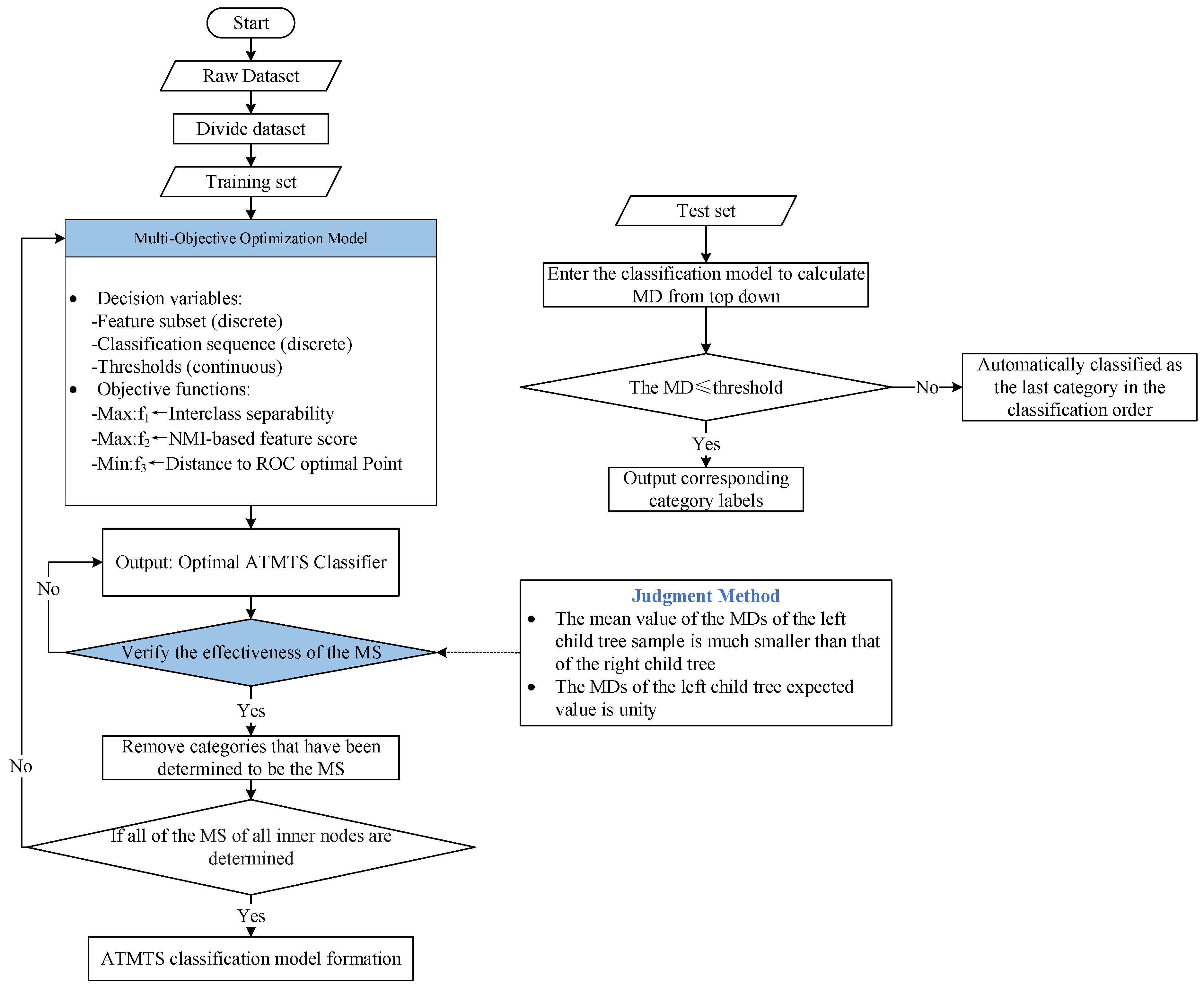
The core innovation of ATMTS is to formulate the construction of an optimal MTS model as a multi-objective optimization problem, which is then solved using a global search algorithm to simultaneously determine the best feature subset, the optimal classification sequence, and the objective threshold.
The overall workflow of the proposed ATMTS framework is illustrated in Figure 4. The process begins with data preprocessing. Subsequently, three critical objectives are defined: (1) maximizing the interclass separability at each node ( f 1 ), (2) maximizing the relevance and minimizing the redundancy of the selected feature subset ( f 2 ), and (3) minimizing the distance between the classifier’s performance and the theoretical optimal point on the ROC curve ( f 3 ). These objectives are integrated into a joint optimization model. The HMOPSO algorithm is employed to efficiently explore the solution space, which includes both continuous (thresholds) and discrete (feature subsets, classification sequence) variables. The output of the optimization is the Pareto-optimal set of solutions, from which the best configuration can be selected to construct a high-performance and robust ATMTS classifier.
The major components of the proposed ATMTS are as follows:
  • An adaptive tree-building mechanism that determines the optimal sequence of dichotomous classifications without relying on pre-defined hierarchical knowledge.
  • A normalized mutual information (NMI)-based criterion for evaluating feature subsets, effectively capturing both linear and nonlinear relationships.
  • An ROC-based objective threshold determination method that minimizes human subjectivity.
  • A joint optimization model that unifies the above components into a single framework.
  • A HMOPSO-based solver designed to handle the mixed-variable optimization problem efficiently.

3.2. Formulation of Objective Functions

The optimization model in ATMTS aims to simultaneously optimize three objectives, defined as follows:
(1)
Interclass separability
Categories that can easily be separated are classified first, thereby reducing the misjudgment of root nodes. Equation (4) is used to obtain categories with high divisibility as follows:
f 1 = i = 1 m t i m , t i = 1 , i f   M D i < min M D j 0 , i f   M D i min M D j , i = 1 , 2 , m
where M D i is the MD of the i -th normal sample, and min M D j is the minimum value of the MD of the abnormal samples. When f 1 = 1 , all the MDs of the normal samples are smaller than the MDs of the abnormal samples. At this time, normal and abnormal samples can be distinguished easily. Thus, the first objective is to maximize f 1 .
(2)
Normalized mutual information
To overcome the limitations of traditional feature selection methods in handling high-dimensional data, and to more precisely serve the feature selection purpose of the MTS, this study adopts a feature selection method based on normalized mutual information (NMI). The core idea of this method is to maximize the nonlinear statistical dependence between features and the target variable while minimizing the nonlinear redundancy among the features themselves [30]. Notably, the traditional feature selection method based on orthogonal arrays and SNR, while demonstrating strong combinatorial search capability through standardized orthogonal tables, suffers from a critical limitation: its search scope is strictly confined to the predefined tabular combinations, failing to cover undefined configurations and consequently lacking statistical completeness. To overcome this critical drawback, our proposed NMI-based approach implements a fundamentally different strategy. It comprehensively evaluates both linear and nonlinear associations between features and targets, establishing a robust statistical foundation for feature prioritization. This methodology enables intelligent guidance of the combinatorial search process, ensuring focus on the most promising feature configurations. Consequently, our approach not only addresses the statistical completeness issue but also yields feature subsets with enhanced robustness and superior discriminative power.
First, the entropy of a variable x k is defined in Equation (5) to measure its uncertainty:
H x k = p x k log 2 p x k
where p x i is the probability distribution function.
The mutual information (MI) between feature x k and x q is then defined by Equation (6):
M I x k , x q = p x k , x q log p x k , x q p x k p x q
where p x k , x q is the joint probability distribution function of random variable x k and random variable x q .
To facilitate comparison across different pairs of variables, the MI value is normalized to the range [0, 1], yielding the normalized mutual information (NMI) as shown in Equation (7):
N M I x k , x q = 2 × M I x k , x q H x k + H x q , 0 N M I 1
The selected features are placed into the feature subset S . The second optimization objective of this study is to find an optimal feature subset S that maximizes the overall relevance to the target variable Y while minimizing the internal redundancy of the subset. Accordingly, the feature evaluation function f 2 is constructed as Equation (8):
f 2 = 1 S N M I x k S x i , Y 2 S S 1 x k , x q S , k < q N M I ( x k , x q )
Here, S denotes the number of features in subset S . A higher value of f 2 indicates better comprehensive quality of the feature subset.
(3)
Proximity to the theoretical optimal point
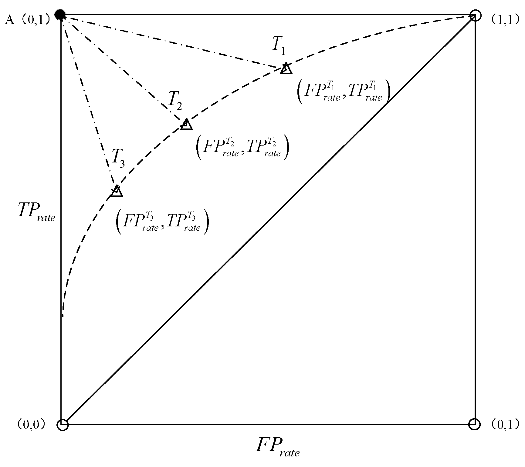
In this paper, we employ the receiver operating characteristic (ROC) curve to determine the threshold, which is more objective and accurate [24]. The ROC curve is illustrated in Figure 5. In Figure 5, the horizontal axis of the curve represents the probability of misclassifying abnormal samples as normal samples, denoted as F P r a t e . The vertical axis represents the probability of correctly classifying normal samples as normal, denoted as T P r a t e . The point (0,1) represents the theoretical optimal point. The curve depicts the classification performance of the MTS under different thresholds T i   i = 1 , 2 , 3 , , n ; changing the threshold will alter the position of the point on the curve. It is evident that the nearer a point is to the theoretical optimal point, the more apt the threshold setting becomes, resulting in enhanced classification performance of the MTS. This observation guides us to the subsequent optimization objective:
f 3 = F P r a t e A F P r a t e T 2 + T P r a t e A T P r a t e T 2
where T P r a t e A = 1 , F P r a t e A = 0 , 0 F P r a t e T 1 , and 0 T P r a t e T 1 . Therefore, the final objective of the optimization model is to minimize f 3 .

3.3. The Joint Optimization Model

Suppose the samples have c categories, p feature variables, and a sample size of n . Let L represent the categories selected for the construction of the MS, S be the subset of feature variables selected during the ATMTS training process, and T be the threshold of the MS, where T 0 represents the initial threshold of the MS; then the optimized model can be expressed as follows:
min y = f L , S , T = [ f 1 L , S , T , f 2 ( L , S ) , f 3 ( L , S , T ) ]
s . t . k = 1 p x k < p k = 1 p x k > 0 M D i = 1 m Z i T C 1 Z i , i = 1 , 2 , m M D j = 1 n m Z j T C 1 Z j , j = m + 1 , m + 2 , n x k 0 , 1 , k = 1 , 2 , p T P r a t e A = 1 F P r a t e A = 0 0 F P r a t e T 1 0 T P r a t e T 1 T 0 = i = 1 m M D i + j = m + 1 n M D j n T P r a t e T = i = 1 m k i m , k i = 1 , i f       M D i T 0 , i = 1 , 2 , , m 0 , i f       M D i > T 0 , i = 1 , 2 , , m F P r a t e T = j = m + 1 n k j n m , k j = 1 , i f       M D j > T 0 , i = m + 1 , m + 2 , , n 0 , i f       M D j T 0 , i = m + 1 , m + 2 , , n

3.4. Model Solving Based on HMOPSO

The joint optimization model presented in this paper addresses the simultaneous refinement of feature selection, classification sequencing, and threshold determination, incorporating both discrete and continuous decision variables. As such, the model is a multi-objective optimization problem of (p + c + 1) dimensions, which is adeptly tackled by the HMOPSO algorithm.
The parameter settings for HMOPSO are chosen based on common practices in the literature [25] and confirmed through preliminary experiments to be effective for our problem. The parameters are as follows: a population size denoted by N = 30, an external repository size capped at M = 100, a maximum iteration threshold of maxIter = 200, a grid partition count set to 50, with each grid harboring an ideal count of 4 particles. Additionally, the inertia weight is calibrated to 0.6, and the individual learning factor c1 and the social learning factor c2 are both fixed at 2, values which are widely accepted and provided stable convergence in our experiments.
The HMOPSO algorithm yields a set of non-dominated solutions forming the Pareto front. To select a single optimal strategy from this front for practical implementation, this paper employs the technique for order preference by TOPSIS [31]. The TOPSIS method operates by first normalizing the objective function values of all Pareto solutions. It then identifies the Positive Ideal Solution (PIS) and the Negative Ideal Solution (NIS). Finally, it calculates the relative closeness of each solution to the PIS and NIS. The solution with the highest closeness degree, representing the best compromise among all objectives, is selected to train the final ATMTS classifier.

3.5. Detailed Implementation Procedure of the ATMTS

The specific implementation steps are outlined as follows:
Step 1: Data Validation Strategy. To ensure robust and reliable performance estimation, a repeated stratified cross-validation scheme is employed rather than a simple random split. Specifically, the 5 × 2 cross-validation design is adopted, involving five replications of a two-fold stratified partitioning. For each replication, one fold is used as the training set while the other serves as the test set, with the roles reversed in the second run.
Step 2: Construct tree hierarchy and MS. Proceeding in a top-down and left-to-right manner throughout the tree structure, determine for each node the MS, the subset of categories belonging to that MS, the classification threshold, and the subset of feature variables used for classification, following the methodology detailed in Section 3.2.
Step 3: Validate the MS. Calculate the MDs for the samples assigned to the left child node and the right child node, respectively. If the mean MD of the samples in the left child node is significantly lower than that of the right child node, and the expected value for the MS is close to unity, then the MS is considered valid. Otherwise, return to Step 2 to reconstruct the MS for the current node.
Step 4: Remove classified categories and iterate. Remove the categories that have been successfully classified. Repeat Steps 2 and 3 for the remaining categories until all leaf nodes contain only a single category, indicating that the MS for all internal nodes in the tree has been finalized.
Step 5: Classify unknown samples. For each sample awaiting classification, calculate its MD starting from the root node and traverse the tree top-down. At each node, compare the sample’s MD with the node’s threshold. If the MD is less than or equal to the threshold, the sample is assigned to the left child node; otherwise, it is assigned to the right child node. The process continues until a leaf node is reached, which provides the final classification result.

4. Data Experiment

4.1. Research Data and Experimental Approach

To demonstrate the efficacy of the ATMTS, we employ five multi-classification datasets sourced from the UCI and Kaggle databases for our analysis. The details of these datasets are provided in Table 1. These five datasets are deliberately selected to construct a rigorous and comprehensive benchmark for evaluating the proposed ATMTS method. The selection criteria cover four principal aspects: diversity in data scale (with sample sizes ranging from 214 to 20,000), variability in feature dimensionality (9 to 18 attributes), a wide spectrum of classification complexity (4 to 26 classes), and representation of distinct real-world domains. Such a strategic selection ensures a robust evaluation of the model’s generalizability and predictive performance. Moreover, the established role of these datasets as standard benchmarks within the machine learning community facilitates direct and meaningful comparisons with a broad range of existing methodologies.
For comparative analysis, several established methods are considered. Specifically, the traditional PBT-MTS and DAG-MTS are included to directly highlight the performance gains achieved by our proposed enhancements. By contrast, the MT-MTS is excluded due to a fundamental limitation: its reliance on a predefined hierarchical taxonomy of sample categories. In practice, such prior structural knowledge is rarely available, as real-world datasets often exhibit flat or unknown class structures. As a result, MT-MTS shows limited generalizability across standard benchmarking scenarios. Moreover, the need to manually construct or source the taxonomy for each new dataset introduces substantial overhead and subjective bias, further reducing its practicality as a general-purpose baseline. In contrast, the proposed ATMTS learns the hierarchical tree structure directly from the data, avoiding these restrictions.
Beyond PBT-MTS, ATMTS is further compared with a comprehensive suite of widely used machine learning algorithms, including Random Forest (RF), Support Vector Machine (SVM), k-Nearest Neighbor (KNN), a Backpropagation Neural Network (BPNN), and AdaBoost, as well as more recent ensemble and deep learning approaches such as XGBoost, LightGBM, CatBoost, and a Convolutional Neural Network (CNN). These methods are chosen to represent diverse methodological paradigms with proven effectiveness: RF, AdaBoost, XGBoost, LightGBM, and CatBoost illustrate the strength of ensemble learning; SVM offers a robust kernel-based decision function; KNN represents a classical instance-based learner; the BPNN provides a shallow neural baseline; and the CNN serves as a deep learning benchmark capable of automatic feature extraction. Collectively, these methods establish a balanced and competitive comparison set, ensuring that the evaluation of ATMTS reflects its advantages relative to both traditional techniques and state-of-the-art approaches.
The hyperparameter settings for each method are specified as follows:
  • ATMTS: Our proposed joint optimization model adaptively determines the classification sequence, feature subset, and decision thresholds.
  • PBT-MTS: Utilizes an orthogonal array and SNR for feature selection, with thresholds set by a Probabilistic Threshold Model (PTM) [32]. The classification order of categories is determined by iteratively calculating the classification accuracy of each category when used as the MS; the category achieving the highest accuracy is prioritized for classification first, and the process continues accordingly.
  • DAG-MTS: This method adopts a DAG as the underlying classification structure in order to improve hierarchical decision-making. Except for the use of the DAG structure, its other procedures are identical to those of PBT-MTS, including feature selection with orthogonal arrays and SNR, threshold determination through the PTM, and the iterative strategy for determining the order of category classification.
  • RF: The key parameters, including the number of trees (Ntree) and the number of features to sample at each split (mtry) are optimized for each dataset via grid search.
  • SVM: A Gaussian Radial Basis Function (RBF) kernel is used. The box constraint C and kernel scale (γ) are optimized for each dataset through grid search.
  • KNN: The number of nearest neighbors (K) is optimized through grid search. The distance metric is set to Euclidean distance.
  • BPNN: A single hidden layer network is used. The number of hidden units (Hiddensize) is determined via grid search.
  • AdaBoost: The algorithm is implemented with decision trees of depth 1 as base learners. The number of estimators (n_estimators) is set by grid search.
  • XGBoost, LightGBM, CatBoost: All hyperparameters, including learning rate (learning_rate) and maximum depth (max_depth) are optimized via grid search within recommended ranges from the literature.
  • CNN: A shallow convolutional architecture is applied. The number of filters (n_filters), kernel sizes (kernel_size) and learning rate (learning_rate) are optimized through grid search.
To ensure fairness in the comparative experiments, we strictly controlled the computational budgets for all methods. Specifically, each algorithm was allocated the same maximum number of evaluations and subjected to identical runtime limits per dataset. The hyperparameter search spaces were also standardized, with all parameter ranges selected based on commonly adopted settings and practical considerations as documented in the literature (see Table 2). This design ensured that no method gained an unfair advantage through a broader search space or longer computation time. Therefore, the observed performance differences can be attributed to the intrinsic effectiveness of the algorithms rather than unequal computational resource allocation [33,34,35,36].
All algorithms were programmed in MATLAB R2019a and run on a standard PC with a Windows 10 OS, an Intel Core i7 2.5 GHz processor, 8 GB of RAM, and 476.92 GB of storage.

4.2. Evaluation Metrics Selection

In this study, we select classification accuracy, Macro-F1, Macro-P, Macro-R, Macro-AUC, multi-class MCC and the Kappa coefficient as the evaluation metrics for the model [37,38]. The definitions are as follows:
A c c u r a c y = i = 1 c c i i i , j = 1 c c i j
M a c r o F 1 = 2 × M a c r o P × M a c r o R M a c r o P + M a c r o R
where M a c r o P = 1 c i = 1 c p r i c i s i o n i ,   M a c r o R = 1 c i = 1 c r e c a l l i ; p r i c i s i o n i = c i i c i , r e c a l l i = c i i c i ; c is the number of categories; c i i are samples with actual labels of i and the classification prediction results are also i ; c i are all the samples with actual labels of i ; and c i are all the samples with classification prediction results of i .
Macro-AUC: The unweighted average of AUCs across all classes, giving equal importance to each class regardless of its size.
Then, the multi-class MCC is given by:
M C C = i = 1 c c i i × N i = 1 c c i × c i N 2 i = 1 c c i 2 × N 2 i = 1 c c i 2
where N is the total number of samples.
K a p p a = p 0 p c 1 p c
where p 0 = i = 1 c c i i i , j = 1 c c i j , p c = i = 1 c c i × c i i , j = 1 c c i j 2 .

4.3. Comprehensive Performance Comparison

4.3.1. Comparative Analysis of Experimental Results

To comprehensively evaluate the effectiveness of the proposed ATMTS, a comparative experiment against several benchmark methods was conducted on five diverse datasets. The detailed experimental results are summarized in Table 3.
The table above compares the performance of the proposed ATMTS method with several classification algorithms across five datasets, using evaluation metrics such as Accuracy, Macro-F1, MCC, and Kappa coefficient. Overall, ATMTS achieves competitive or superior results in most cases, performing particularly well on the Letter Recognition, Page Blocks, and Vehicle datasets. Compared to traditional tree-based methods such as PBT-MTS and DAG-MTS, ATMTS shows consistent improvement across all datasets, indicating its enhanced classification efficiency and structural adaptability. When evaluated against ensemble methods like RF, XGBoost, and LightGBM, ATMTS remains highly competitive, and it also performs comparably to deep learning approaches such as the CNN, underscoring the effectiveness of its joint optimization in feature selection and classification. Even on more challenging tasks such as White Wine Quality, ATMTS maintains robust performance, demonstrating its strong generalization capability and reliability.

4.3.2. Statistical Significance Testing

To comprehensively compare the different classification methods, the Friedman test was employed to assess whether there are statistically significant differences among the methods across multiple datasets. For each dataset, the methods are ranked based on their performance, with the best-performing method assigned rank 1, the next best rank 2, and so on. The null hypothesis of the Friedman test states that all methods perform equivalently. In our experiments, the significance level is set to 0.05. If the Friedman test rejects the null hypothesis, indicating significant differences, the Holm post hoc test is subsequently applied for pairwise comparisons. In the Holm test, the procedure is sequential: if a given null hypothesis cannot be rejected, all remaining hypotheses are also not rejected [39].
The Friedman test results (Table 4) indicate that performance differences among the different classification methods are statistically significant (p < 0.05) across all five datasets. Consequently, we further performed the Holm post hoc test, focusing on the pairwise comparisons between the ATMTS method and other classifiers. As shown in Table 5, ATMTS demonstrated significant advantages (p < 0.05) over the traditional tree-structured methods PBT-MTS and DAG-MTS across all datasets, with effect sizes ranging from medium to large. Particularly on the Letter Recognition and Page-blocks datasets, ATMTS showed the greatest improvement over PBT-MTS (δ > 0.54). Compared to popular algorithms such as RF and SVM, ATMTS also exhibited significant superiority in most cases; for instance, comparisons against both RF and SVM on the Vehicle dataset reached significance. These results consistently demonstrate that the ATMTS method significantly outperforms the comparative methods in classification performance, and its proposed joint optimization strategy effectively enhances the classifier’s generalization capability.

4.3.3. Comparative Analysis with Existing Studies

To further substantiate the effectiveness of the proposed approach, we compared our experimental outcomes with those reported in prior studies on the same benchmark datasets [41,42,43]. Existing literature indicates that the performance of mainstream classifiers on the Letter Recognition dataset generally ranges between 90% and 97%, while on the Wine Quality dataset, accuracies are typically observed within the 70–75% interval. For the Glass dataset, reported results usually fall in the 60–80% range, whereas Page-blocks yields relatively higher accuracies, often approaching 95%. In contrast, the Vehicle dataset has been shown to achieve accuracies of approximately 70–85% depending on the method applied. The performance of our proposed method consistently reached the relatively higher end of these documented ranges across all benchmarks, demonstrating its competitive and robust capability compared to established approaches.

4.3.4. Computational Complexity Comparison

We further evaluate the practical applicability of the proposed method by analyzing its computational complexity relative to established classification algorithms [44,45]. The training complexity of ATMTS is governed by binary tree construction and node-level iterative optimization. For a dataset with c classes, the tree contains O(c) nodes in the worst case. The feature selection and hyperparameter tuning at each node contribute approximately O(n·d·k), where n is the number of samples, d the feature dimensionality, and k the number of iterations. This leads to an overall worst-case training complexity of O(c·n·d·k). While this exceeds the O(1) training complexity of instance-based methods like KNN, it remains competitive with other advanced approaches.
Compared to ATMTS, SVM typically exhibits O(n2) to O(n3) training complexity, while RF maintains approximately O(m·n·d·log n), where m represents the number of trees. Modern gradient boosting methods including XGBoost and LightGBM achieve similar asymptotic complexity with improved constants owing to algorithmic optimizations. The CNN generally scales as O(e·n·d·h), with e and h denoting the number of training epochs and network depth, respectively.
The principal advantage of ATMTS emerges during the inference stage, where its prediction complexity is only O(depth·d), or approximately O(log c·d) under a balanced tree structure. This represents a substantial efficiency improvement over instance-based methods such as KNN (O(n·d) per query), ensemble methods like RF (O(m·depth·d)), and deep architectures including the CNN (O(h·d)).
In summary, ATMTS achieves a favorable balance between classification accuracy and computational efficiency. It accepts a manageable training overhead to build an effective and scalable prediction model, rendering it particularly suitable for real-world applications that demand both high predictive performance and rapid inference capability.

4.3.5. Model Interpretability Analysis

Beyond computational efficiency, another key strength of the proposed ATMTS method lies in its intrinsic interpretability, which addresses one of the most persistent challenges in modern machine learning models. Unlike many black-box classifiers, ATMTS provides both transparent global decision logic and clear local interpretive paths for individual samples. Its multi-branch hierarchical tree structure allows each decision to be decomposed into interpretable node-level rules, while the classification route of any instance remains fully traceable—enabling genuinely “white-box” decision-making.
In contrast, the benchmark algorithms considered in this study generally exhibit limited interpretability. Although both PBT-MTS and DAG-MTS are tree-related models with clearly defined decision paths, their overall interpretability remains somewhat constrained. The sequential structure of PBT-MTS provides a clear but rigid decision process, limiting its flexibility in representing complex category relationships. In contrast, the graph-based configuration of DAG-MTS introduces higher structural complexity, making the global decision logic less intuitive to analyze or visualize. Compared with these approaches, ATMTS achieves a better balance between interpretability and adaptability through its hierarchically organized and self-optimized tree structure.
Traditional and ensemble approaches such as SVM, the BPNN, RF, and gradient boosting models (e.g., XGBoost, LightGBM, CatBoost) largely operate as black- or grey-box systems, producing accurate predictions through high-dimensional transformations or aggregated weak learners, but offering little insight into how individual decisions are made. Deep learning architectures such as the CNN exhibit the lowest transparency, as their decision mechanisms rely on intricate layer-wise feature abstractions that are difficult to interpret even with post hoc visualization techniques.

4.4. Performance Comparison Between ATMTS, PBT-MTS, and DAG-MTS

Using the Vehicle dataset, which contains four categories (BUS, VAN, OPEL, and SAAB) as a typical case, a detailed comparison between ATMTS, PBT-MTS, and DAG-MTS was performed. It is important to note that, although the model evaluation was conducted using multi-round cross-validation, the results from a single, representative data split are presented here for detailed comparison and visualization. This approach allowed for a clear and concrete illustration of the performance differences among the methods.
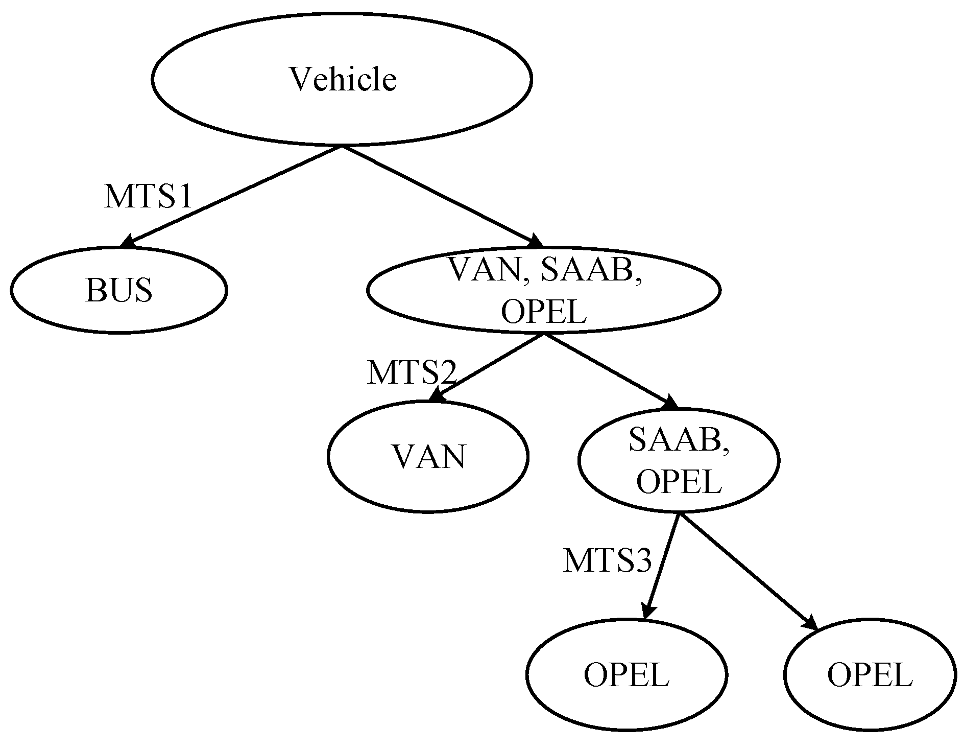
The proposed ATMTS framework first identifies the optimal root node classification. The VAN and BUS categories are selected to form the MS at the root node, with the corresponding classifier designated as MTS1. Following a top-down, left-to-right adaptive tree-building process, the VAN category is further distinguished as the MS of the left subtree, with its associated classifier labeled MTS2. Concurrently, the SAAB category is identified as the MS for the right subtree, and its classifier is denoted as MTS3. This iterative process continues until all leaf nodes contain only a single category, thereby completing the classification model, whose final architecture is presented in Figure 6. The objectively determined thresholds for MTS1, MTS2, and MTS3 are 1.7073, 2.3583, and 1.4248, respectively. The feature selection results are presented in Table 6.
In contrast, the traditional PBT-MTS method employs a fixed one-versus-all strategy with a classification sequence: BUS, VAN, OPEL, and SAAB, as shown in Figure 7. The thresholds for its classifiers MTS1, MTS2, and MTS3, calculated using the PTM, are 1.5432, 1.8062, and 1.3654, respectively. The feature selection results can be found in Table 7.
Based on the structural representation in Figure 8, the DAG-MTS classification model employs a directed acyclic graph architecture comprising six intermediate nodes. The model constructs a complex decision network through six binary classifiers: BUS vs. VAN, BUS vs. OPEL, SAAB vs. VAN, BUS vs. SAAB, SAAB vs. OPEL, and OPEL vs. VAN. The decision thresholds for each classifier, optimized through our methodology, are determined as 1.654, 1.893, 2.127, 1.742, 1.985, and 2.034, respectively. The complete feature selection results are detailed in Table 8.
A key advantage of the ATMTS approach is its ability to construct independent subtrees. In this case, the classifications performed by MTS2 and MTS3 are mutually independent and can be executed in parallel. This inherent parallelism significantly enhances computational efficiency compared to the strictly sequential classification process required by PBT-MTS. While DAG-MTS also supports parallel processing to some extent, it requires a significantly larger number of classifiers (six in this instance) to implement its directed acyclic graph structure, resulting in substantially increased training complexity and resource requirements. This case study convincingly demonstrates that ATMTS achieves superior computational efficiency compared to both the strictly sequential PBT-MTS and the more complex DAG-MTS, while maintaining competitive classification accuracy with a more streamlined architecture.
To quantitatively validate the computational efficiency of ATMTS, we compared its runtime performance with both PBT-MTS and DAG-MTS under identical conditions. The traditional PBT-MTS requires strictly sequential execution of its classification nodes MTS1–MTS2–MTS3, resulting in a total inference time of 18.7 s. The DAG-MTS approach employed six classifiers in its graph structure, achieving partial parallelism but still requiring 15.2 s due to coordination overhead and increased computational load.
In contrast, ATMTS completed the classification task in just 11.3 s by executing independent subtrees in parallel. This represents a 39.6% speedup over PBT-MTS and a 25.7% improvement over DAG-MTS. The results clearly demonstrate that ATMTS achieves superior computational efficiency while maintaining competitive accuracy, making it particularly suitable for applications requiring rapid inference.

4.5. Validation of Optimization Model Effectiveness

To provide a concrete demonstration of the optimization model’s effectiveness, a detailed case study was conducted using the white wine quality dataset. This dataset, with its multiple ordered quality classes, serves as an ideal benchmark to illustrate how the proposed ATMTS adaptively constructs the MS and validates its rationality. For clarity in comparative analysis, this section presents results from one representative cross-validation fold.
In this dataset, the classification labels consisted of seven quality levels: 3, 4, 5, 6, 7, 8, and 9. The first MS was constructed using quality levels 6, 7, 8, and 9 as the normal group, while levels 3, 4, and 5 were designated as abnormal samples. The corresponding classifier was denoted as MTS1. Validation of MTS1 confirmed that the expected value of the MDs for the normal group was 0.9988, satisfying the theoretical requirement of being close to unity. Furthermore, as shown in Figure 9a, the MDs of the normal samples in MTS1 were significantly smaller than those of the abnormal samples, demonstrating the rationality of the MTS1 construction.
Subsequently, the left subtree (containing quality levels 6, 7, 8, and 9) was further partitioned to determine its classification sequence. Using the proposed optimization strategy, quality level 6 was selected to form the MS, with levels 7, 8, and 9 treated as abnormal samples. This configuration achieved the highest closeness degree, and the corresponding classifier is labeled MTS2. The classification sequence for levels 7, 8, and 9 was then optimized, resulting in the construction of an MS with quality level 7 (abnormal samples: 8 and 9); the corresponding classifier was denoted as MTS3. Finally, an MS was constructed using quality level 9 (abnormal sample: 8), yielding the trained classifier MTS4.
Similarly, the classification sequence for the right subtree (containing quality levels 3, 4, and 5) was determined. Based on the calculated closeness degree, quality level 3 was chosen to construct the MS, with the remaining samples treated as abnormal; the resulting classifier was designated MTS5. Further analysis of levels 4 and 5 led to the construction of an MS with quality level 5, and the corresponding classifier is denoted as MTS6.
It is important to emphasize that the MS constructed in this study can adaptively incorporate samples from multiple categories, overcoming the limitation of traditional MTS where the MS is confined to a single category. The validation results confirm that this innovation not only remains effective but also enhances classification efficiency.
The rationality of MTS2 to MTS6 was validated, and the results are presented in Figure 9b–f. The expected values for these MS are 0.9991, 0.9924, 0.9994, 0.9986, and 0.9926, respectively, all satisfying the theoretical condition of being close to unity. Additionally, the MDs of the vast majority of abnormal samples are significantly distinct from those of the normal samples, indicating that the MS constructions are rational and capable of effectively identifying abnormal samples.
As the depth of the binary tree classification structure increases, a continuous reduction in the MDs between normal and abnormal samples is observed. This trend corroborates the effectiveness of the proposed strategy, which prioritizes placing more easily distinguishable categories at the root node for classification. Compared to traditional fixed classification structures (e.g., one-vs-rest), our method establishes a more flexible and efficient classification pathway, in which multiple classifiers can be executed in parallel, thereby enhancing both classification accuracy and computational efficiency.
Furthermore, to quantitatively isolate and evaluate the causal contribution of each core module within the ATMTS framework, a comprehensive ablation study was conducted. Using the wine quality dataset, the performance of the ATMTS model was rigorously compared against the following two variants:
Variant A (w/o NMI): This variant replaces the NMI-based feature selection with the orthogonal array and signal-to-noise ratio method, thereby isolating the impact of the proposed feature selection mechanism.
Variant B (w/o ROC-based Objective): This variant substitutes the ROC analysis for threshold determination with the PTM method, isolating the effect of the optimized threshold learning process.
The results demonstrate that both the NMI-based feature selection and the ROC-based threshold optimization contribute significantly to the model’s performance. Quantitative analysis reveals that removing the NMI feature selection (Variant A) causes an MCC decrease of 0.036 (5.0% relative drop), while eliminating the ROC threshold optimization (Variant B) leads to an MCC reduction of 0.023 (3.2% relative drop).

5. Conclusions and Future Outlook

Due to the use of a unique and overall MS in the conventional multi-class MTS, the traditional tree-structured MTS, commonly referred to as PBT-MTS, can only identify one category of samples at a time. In contrast, the DAG-MTS offers more flexible decision paths through its graph structure but requires constructing significantly more classifier nodes, substantially increasing model complexity and computational overhead. Both traditional methods prove suboptimal in diverse data environments. For instance, as the number of sample categories increases, PBT-MTS experiences significant growth in tree depth leading to decreased classification efficiency, while DAG-MTS faces rapidly escalating computational complexity.
Reflecting on the current work, the primary advantage of ATMTS lies in its adaptive tree-building process. By analyzing samples through a joint optimization model, we construct a multi-classification system based on an adaptive binary tree that overcomes both the rigid structural limitations of PBT-MTS and the excessive complexity of DAG-MTS. Simultaneously, this method automatically determines the optimal classification sequence, feature variable subset, and threshold values. Experiments across multiple datasets demonstrate that our approach not only achieves better classification performance than both PBT-MTS and DAG-MTS but also enables more efficient feature selection. Compared to these traditional methods, ATMTS allows multiple classifiers to operate in parallel, resulting in higher classification efficiency.
Therefore, this method helps improve the accuracy and generalization performance of MTS on multi-classification problems while also advancing the theoretical framework of MTS. However, due to iterative optimization and tree construction, the computational cost during the training phase remains higher than that of simple baseline models.
This method shows direct application potential in multiple real-world scenarios, including defect classification in industrial quality inspection, relative poverty identification in public policy domains, and evaluation of teaching–research integrated academic talent in higher education institutions. Future work will focus on developing more efficient hierarchical strategies and validating ATMTS in these practical scenarios to enhance its impact on real-world decision-making.

Author Contributions

Conceptualization, Y.S. and Y.C.; methodology, Y.S.; software, Y.X.; validation, Y.S.; formal analysis, Y.C.; data curation, Y.S.; writing—original draft preparation, Y.S.; writing—review and editing, Y.S. and Y.X.; visualization, Y.C.; supervision, Y.X.; project administration, Y.C.; funding acquisition, Y.S. All authors have read and agreed to the published version of the manuscript.

Funding

This research was funded by Zhejiang Province Educational Science Planning Project: Research on a Multi-Dimensional Evaluation System for University Talent with Equal Emphasis on Teaching and Research Under Multi-Source Heterogeneous Data Fusion, grant number 2024SCG422.

Data Availability Statement

The data presented in this study are openly available in the UCI Machine Learning Repository at https://archive.ics.uci.edu/ml/datasets (accessed on 20 October 2024) and in the Kaggle database at https://www.kaggle.com/datasets (accessed on 20 October 2024).

Acknowledgments

The authors would like to express sincere gratitude to College of Modern Science and Technology from China Jiliang University. During the preparation of this work the authors used DeepSeek in order to improve language. After using this tool, the authors reviewed and edited the content as needed and take full responsibility for the content of the publication.

Conflicts of Interest

The authors declare no conflicts of interest.

References

  1. Ma, S.; Shi, S.; Zhang, Y.; Gao, H. A High-precision method for detecting rolling bearing faultis in unmanned aerial vehicle based on improved 1DCNN-Informer model. Measurement 2025, 256, 118200. [Google Scholar] [CrossRef]
  2. Wang, Y.; Du, X. Rolling Bearing Fault Diagnosis Based on SCNN and Optimized HKELM. Mathematics 2025, 13, 2004. [Google Scholar] [CrossRef]
  3. Xiu, X.C.; Pan, L.L.; Yang, Y.; Liu, W.Q. Efficient and Fast Joint Sparse Constrained Canonical Correlation Analysis for Fault Detection. IEEE Trans. Neural Netw. Learn. Syst. 2024, 35, 4153–4163. [Google Scholar] [CrossRef] [PubMed]
  4. Razavi-Termeh, S.V.; Bazargani, J.S.; Sadeghi-Niaraki, A.; Angela Yao, X.; Choi, S.-M. Spatial prediction and visualization of PM 2.5 susceptibility using machine learning optimization in a virtual reality environment. Int. J. Digit. Earth 2025, 18, 2513589. [Google Scholar] [CrossRef]
  5. Jyotiyana, M.; Kesswani, N.; Kumar, M. A deep learning approach for classification and diagnosis of Parkinson’s disease. Soft Comput. 2022, 26, 9155–9165. [Google Scholar] [CrossRef]
  6. Wu, Z.; Zhou, C.; Xu, F.; Lou, W. A CS-AdaBoost-BP model for product quality inspection. Ann. Oper. Res. 2022, 308, 685–701. [Google Scholar] [CrossRef]
  7. Heo, W.; Kim, E. Smoothing the Subjective Financial Risk Tolerance: Volatility and Market Implications. Mathematics 2025, 13, 680. [Google Scholar] [CrossRef]
  8. Chang, Z.P.; Li, Y.W.; Fatima, N. A theoretical survey on Mahalanobis-Taguchi system. Measurement 2019, 136, 501–510. [Google Scholar] [CrossRef]
  9. Su, C.T.; Hsiao, Y.H. Multiclass MTS for Simultaneous Feature Selection and Classification. IEEE Trans. Knowl. Data Eng. 2009, 21, 192–205. [Google Scholar]
  10. Shimura, J.; Takata, D.; Watanabe, H.; Shitanda, I.; Itagaki, M. Mahalanobis-Taguchi method based anomaly detection for lithium-ion battery. Electrochim. Acta 2024, 479, 143890. [Google Scholar] [CrossRef]
  11. Zhang, C.H.; Cheng, X.R.; Li, K.; Li, B. Hotel recommendation mechanism based on online reviews considering multi-attribute cooperative and interactive characteristics. Omega-Int. J. Manage S 2025, 130, 103173. [Google Scholar] [CrossRef]
  12. Sikder, S.; Mukherjee, I.; Panja, S.C. A synergistic Mahalanobis-Taguchi system and support vector regression based predictive multivariate manufacturing process quality control approach. J. Manuf. Syst. 2020, 57, 323–337. [Google Scholar] [CrossRef]
  13. Halim, N.A.M.; Abu, M.Y.; Razali, N.S.; Aris, N.H.; Sari, E.; Jaafar, N.N.; Ghani, A.S.A.; Ramlie, F.; Muhamad, W.Z.A.W.; Harudin, N. Impact of Mahalanobis-Taguchi System on Health Performance Among Academicians. Int. J. Technol. 2025, 16, 846–864. [Google Scholar] [CrossRef]
  14. Hsiao, Y.H.; Su, C.T. Multiclass MTS for Saxophone Timbre Quality Inspection Using Waveform-shape-based Features. IEEE Trans. Syst. Man. Cybern. B Cybern. 2009, 39, 690–704. [Google Scholar] [CrossRef] [PubMed]
  15. Soylemezoglu, A.; Jagannathan, S.; Saygin, C. Mahalanobis Taguchi System (MTS) as a Prognostics Tool for Rolling Element Bearing Failures. J. Manuf. Sci. E-T Asme 2010, 132, 051014. [Google Scholar] [CrossRef]
  16. Peng, Z.M.; Cheng, L.S.; Zhan, J.; Yao, Q.F. Fault classification method for rolling bearings based on the multi-featureextraction and modified Mahalanobis-Taguchi system. J. Vib. Shock 2020, 39, 249–256. [Google Scholar]
  17. Peng, Z.; Cheng, L.; Yao, Q. Multi-feature Extraction for Bearing Fault Diagnosis Using Binary-tree Mahalanobis-Taguchi System. In Proceedings of the 31st Chinese Control And Decision Conference (CCDC), Nanchang, China, 3–5 June 2019; pp. 3303–3308. [Google Scholar]
  18. Zhan, J.; Cheng, L.; Peng, Z. Rolling Bearings Fault Diagnosis Using VMD and Multi-tree Mahalanobis Taguchi System. IOP Conf. Ser. Mater. Sci. Eng. 2019, 692, 12034–12043. [Google Scholar] [CrossRef]
  19. Duan, Y.; Zou, B.; Xu, J.; Chen, F.; Wei, J.; Tang, Y.Y. OAA-SVM-MS: A fast and efficient multi-class classification algorithm. Neurocomputing 2021, 454, 448–460. [Google Scholar] [CrossRef]
  20. Tan, L.M.; Wan Muhamad, W.Z.A.; Yahya, Z.R.; Junoh, A.K.; Azziz, N.H.A.; Ramlie, F.; Harudin, N.; Abu, M.Y.; Tan, X.J. A survey on improvement of Mahalanobis Taguchi system and its application. Multimed. Tools Appl. 2023, 82, 43865–43881. [Google Scholar] [CrossRef]
  21. Chang, Z.; Wang, Y.; Chen, W. Dynamic Identification of Relative Poverty Among Chinese Households Using the Multiway Mahalanobis–Taguchi System: A Sustainable Livelihoods Perspective. Sustainability 2025, 17, 5384. [Google Scholar] [CrossRef]
  22. Huang, C.-L.; Hsu, T.-S.; Liu, C.-M. The Mahalanobis-Taguchi system—Neural network algorithm for data-mining in dynamic environments. Expert. Syst. Appl. 2009, 36, 5475–5480. [Google Scholar] [CrossRef]
  23. Luo, Y.; Zou, X.; Xiong, W.; Yuan, X.; Xu, K.; Xin, Y.; Zhang, R. Dynamic State Evaluation Method of Power Transformer Based on Mahalanobis–Taguchi System and Health Index. Energies 2023, 16, 2765. [Google Scholar] [CrossRef]
  24. Ramlie, F.; Muhamad, W.Z.A.W.; Harudin, N.; Abu, M.Y.; Yahaya, H.; Jamaludin, K.R.; Abdul Talib, H.H. Classification Performance of Thresholding Methods in the Mahalanobis-Taguchi System. Appl. Sci. 2021, 11, 3906. [Google Scholar] [CrossRef]
  25. Yang, M.; Liu, Y.; Yang, J.; Precup, R.-E. A Hybrid Multi-Objective Particle Swarm Optimization with Central Control Strategy. Comput. Intell. Neurosci. 2022, 2022, 1522096. [Google Scholar] [CrossRef]
  26. Hao, H.Q.; Zhu, H.P.; Luo, Y.B. Preference learning based multiobjective particle swarm optimization for lot streaming in hybrid flowshop scheduling with flexible assembly and time windows. Expert. Syst. Appl. 2025, 290, 128345. [Google Scholar] [CrossRef]
  27. Woodall, W.H.; Koudelik, R.; Tsui, K.-L.; Kim, S.B.; Stoumbos, Z.G.; Carvounis, C.P. A Review and Analysis of the Mahalanobis—Taguchi System. Technometrics 2003, 45, 1–15. [Google Scholar] [CrossRef]
  28. Iquebal, A.S.; Pal, A.; Ceglarek, D.; Tiwari, M.K. Enhancement of Mahalanobis-Taguchi System via Rough Sets based Feature Selection. Expert. Syst. Appl. 2014, 41, 8003–8015. [Google Scholar] [CrossRef]
  29. Kim, S.-G.; Park, D.; Jung, J.-Y. Evaluation of One-Class Classifiers for Fault Detection: Mahalanobis Classifiers and the Mahalanobis-Taguchi System. Processes 2021, 9, 1450. [Google Scholar] [CrossRef]
  30. Hassan, M.S.; Chin, V.J.; Gopal, L. Accurate diagnosis of concurrent faults in photovoltaic systems using CONMI-based feature selection and Support vector machines. Energy Convers. Manag. 2025, 344, 120293. [Google Scholar] [CrossRef]
  31. Wang, C.; Shi, J.; Yang, Y.; Wang, R. Two Methods With Bidirectional Similarity for Optimal Selections of Supplier Portfolio and Supplier Substitute Based on TOPSIS and IFS. IEEE Access 2024, 12, 1761–1773. [Google Scholar] [CrossRef]
  32. Su, C.T.; Hsiao, Y.H. An Evaluation of the Robustness of MTS for Imbalanced Data. IEEE Trans. Knowl. Data Eng. 2007, 19, 1321–1332. [Google Scholar] [CrossRef]
  33. Demir, S.; Sahin, E.K. Predicting occurrence of liquefaction-induced lateral spreading using gradient boosting algorithms integrated with particle swarm optimization: PSO-XGBoost, PSO-LightGBM, and PSO-CatBoost. Acta Geotech. 2023, 18, 3403–3419. [Google Scholar] [CrossRef]
  34. Le Nguyen, K.; Shakouri, M.; Ho, L.S. Investigating the effectiveness of hybrid gradient boosting models and optimization algorithms for concrete strength prediction. Eng. Appl. Artif. Intel. 2025, 149, 110568. [Google Scholar]
  35. Sun, Y.; Gong, J.; Zhang, Y. A Multi-Classification Method Based on Optimized Binary Tree Mahalanobis-Taguchi System for Imbalanced Data. Appl. Sci. 2022, 12, 10179. [Google Scholar] [CrossRef]
  36. Bentéjac, C.; Csörgő, A.; Martínez-Muñoz, G. A comparative analysis of gradient boosting algorithms. Artif. Intel. Rev. 2020, 54, 1937–1967. [Google Scholar] [CrossRef]
  37. Kucukosmanoglu, M.; Garcia, J.O.; Brooks, J.; Bansal, K. Influence of cognitive networks and task performance on fMRI-based state classification using DNN models. Sci. Rep. 2025, 15, 23689. [Google Scholar] [CrossRef]
  38. Qaedi, K.; Abdullah, M.; Yusof, K.A.; Hayakawa, M.; Zulhamidi, N.F.I. Multi-class classification automated machine learning for predicting earthquakes using global geomagnetic field data. Nat. Hazards 2025, 121, 14531–14544. [Google Scholar] [CrossRef]
  39. Solorio-Fernández, S.; Carrasco-Ochoa, J.A.; Martínez-Trinidad, J.F. A systematic evaluation of filter Unsupervised Feature Selection methods. Expert. Syst. Appl. 2020, 162, 113745. [Google Scholar] [CrossRef]
  40. Bais, F.; van der Neut, J. Adapting the Robust Effect Size Cliff’s Delta to Compare Behaviour Profiles. Surv. Res. Methods 2022, 16, 329–352. [Google Scholar]
  41. Renkas, K.; Niewiadomski, A. Hierarchical Fuzzy Logic Systems in Classification: An Application Example. In Proceedings of the 16th International Conference on Artificial Intelligence and Soft Computing (ICAISC), Zakopane, Poland, 11–15 June 2017; pp. 302–314. [Google Scholar]
  42. Alharbi, N.M.; Osman, A.H.; Mashat, A.A.; Alyamani, H.J. Letter Recognition Reinvented: A Dual Approach with MLP Neural Network and Anomaly Detection. Comput. Syst. Sci. Eng. 2024, 48, 175–198. [Google Scholar] [CrossRef]
  43. Xu, C.; Wang, Y.; Bao, X.; Li, F. Vehicle Classification Using an Imbalanced Dataset Based on a Single Magnetic Sensor. Sensors 2018, 18, 1690. [Google Scholar] [CrossRef] [PubMed]
  44. Ma, Y.F.; Liang, X.; Sheng, G.; Kwok, J.T.; Wang, M.L.; Li, G.S. Noniterative Sparse LS-SVM Based on Globally Representative Point Selection. IEEE Trans. Neural Netw. Learn. Syst. 2021, 32, 788–798. [Google Scholar] [CrossRef] [PubMed]
  45. Chen, T.; Guestrin, C. XGBoost: A Scalable Tree Boosting System. In Proceedings of the 22nd ACM SIGKDD International Conference on Knowledge Discovery and Data Mining, San Francisco, CA, USA, 13–17 August 2016; pp. 785–794. [Google Scholar]
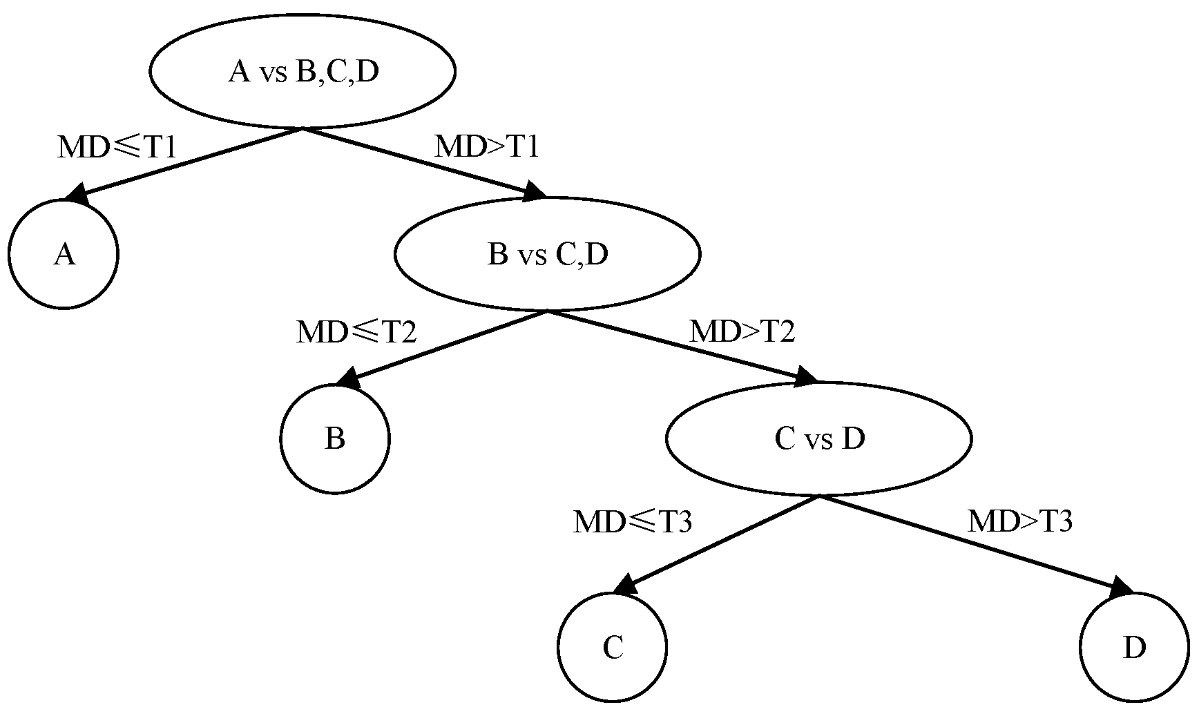
Figure 1. Schematic of the fixed one-versus-all binary tree in PBT-MTS.
Mathematics 13 03233 g001
Figure 2. Multi-classification model of MT-MTS based on a predefined taxonomy.
Mathematics 13 03233 g002
Figure 3. The DAG-MTS approach to a 4-class classification problem.
Mathematics 13 03233 g003
Figure 4. The overall framework of the ATMTS.
Mathematics 13 03233 g004
Figure 5. Threshold locations on the ROC curve.
Mathematics 13 03233 g005
Figure 6. The ATMTS classification model for the vehicle dataset.
Mathematics 13 03233 g006
Figure 7. The PBT-MTS classification model for the vehicle dataset.
Mathematics 13 03233 g007
Figure 8. The DAG-MTS classification model for the vehicle dataset.
Mathematics 13 03233 g008
Figure 9. Performance comparison of MS (MTS1-MTS6) on the wine quality dataset.
Mathematics 13 03233 g009
Table 1. Dataset information.
DatasetNumber of SamplesNumber of Feature VariablesNumber of Categories
Letter Recognition20,0001626
White wine quality4898117
Glass21496
Page-blocks5437105
Vehicle846184
Table 2. Search ranges for all hyperparameters in the grid search for RF, SVM, KNN, the BPNN, AdaBoost, XGBoost, LightGBM, CatBoost and the CNN.
MethodHyper-ParameterGrid Search Values
RFNtree
mtry
50–500 (step size 50)
2, 5, 10, 20
SVMC
γ
2−8–28 (step size: 1)
KNNK1–20 (step size: 1)
BPNNHiddensize n + m + a , where n is number of input nodes, m is number of output nodes, a = 1−10 (step size: 1)
Adaboostn_estimators50–500 (step size: 50)
XGboostlearning_rate
max_depth
0.025, 0.05, 0.1, 0.2, 0.3
1–6 (step size 1)
LightGBMlearning_rate
max_depth
0.025, 0.05, 0.1, 0.2, 0.3
2–10 (step size: 1)
CatBoostlearning_rate
max_depth
0.025, 0.05, 0.1, 0.2, 0.3
1–10 (step size: 1)
CNNn_filters
kernel_size
learning_rate
16, 32, 64
3, 5, 7
0.025, 0.05, 0.1, 0.2, 0.3
Table 3. Classification performance comparison of different methods.
DatasetMethodEvaluation Index
AccuracyMacro-F1Macro-RMacro-PMCCMacro-AUCKappa Coefficient
Letter RecognitionATMTS0.976 ± 0.0030.955 ± 0.0050.945 ± 0.0020.964 ± 0.0040.945 ± 0.0030.960 ± 0.0050.944 ± 0.003
PBT-MTS0.937 ± 0.0050.915 ± 0.0040.906 ± 0.0030.925 ± 0.0050.905 ± 0.0040.921 ± 0.0050.904 ± 0.004
DAG-MTS0.950 ± 0.0040.929 ± 0.0030.919 ± 0.0030.938 ± 0.0030.919 ± 0.0030.934 ± 0.0040.918 ± 0.005
RF0.960 ± 0.0040.939 ± 0.0050.930 ± 0.0050.948 ± 0.0030.929 ± 0.0040.945 ± 0.0040.929 ± 0.003
SVM0.947 ± 0.0040.926 ± 0.0050.916 ± 0.0050.936 ± 0.0050.915 ± 0.0040.931 ± 0.0050.915 ± 0.002
KNN0.957 ± 0.0040.936 ± 0.0050.928 ± 0.0040.944 ± 0.0050.927 ± 0.0030.941 ± 0.0040.926 ± 0.003
BPNN0.944 ± 0.0030.922 ± 0.0050.913 ± 0.0050.932 ± 0.0030.912 ± 0.0030.928 ± 0.0050.912 ± 0.004
AdaBoost0.935 ± 0.0050.914 ± 0.0040.904 ± 0.0020.924 ± 0.0030.904 ± 0.0030.920 ± 0.0040.903 ± 0.005
XGBoost0.961 ± 0.0050.940 ± 0.0040.931 ± 0.0040.950 ± 0.0050.930 ± 0.0030.946 ± 0.0030.929 ± 0.004
LightGBM0.953 ± 0.0040.932 ± 0.0040.923 ± 0.0030.942 ± 0.0050.922 ± 0.0030.938 ± 0.0030.921 ± 0.004
CatBoost0.968 ± 0.0040.947 ± 0.0030.937 ± 0.0030.957 ± 0.0020.937 ± 0.0030.952 ± 0.0040.936 ± 0.003
CNN0.969 ± 0.0030.948 ± 0.0050.938 ± 0.0050.957 ± 0.0050.938 ± 0.0030.953 ± 0.0030.937 ± 0.003
White wine qualityATMTS0.682 ± 0.0070.661 ± 0.0050.652 ± 0.0100.670 ± 0.0110.651 ± 0.0080.666 ± 0.0050.650 ± 0.011
PBT-MTS0.653 ± 0.0090.632 ± 0.0050.623 ± 0.0050.641 ± 0.0120.622 ± 0.0070.637 ± 0.0050.621 ± 0.005
DAG-MTS0.661 ± 0.0100.640 ± 0.0060.631 ± 0.0100.649 ± 0.0070.630 ± 0.0060.645 ± 0.0090.629 ± 0.012
RF0.667 ± 0.0100.646 ± 0.0100.637 ± 0.0100.655 ± 0.0060.636 ± 0.0070.651 ± 0.0060.635 ± 0.004
SVM0.664 ± 0.0110.643 ± 0.0070.634 ± 0.0090.652 ± 0.0070.633 ± 0.0050.648 ± 0.0120.632 ± 0.005
KNN0.657 ± 0.0110.636 ± 0.0060.627 ± 0.0070.645 ± 0.0100.626 ± 0.0060.641 ± 0.0070.625 ± 0.008
BPNN0.672 ± 0.0070.651 ± 0.0090.642 ± 0.0080.660 ± 0.0090.641 ± 0.0100.656 ± 0.0090.640 ± 0.005
AdaBoost0.671 ± 0.0060.650 ± 0.0050.641 ± 0.0070.659 ± 0.0050.640 ± 0.0090.655 ± 0.0080.639 ± 0.012
XGBoost0.664 ± 0.0080.643 ± 0.0060.634 ± 0.0070.652 ± 0.0110.633 ± 0.0070.648 ± 0.0120.632 ± 0.009
LightGBM0.680 ± 0.0090.659 ± 0.0110.650 ± 0.0100.668 ± 0.0080.649 ± 0.0110.664 ± 0.0110.648 ± 0.005
CatBoost0.680 ± 0.0100.659 ± 0.0110.649 ± 0.0080.668 ± 0.0080.649 ± 0.0060.664 ± 0.0050.648 ± 0.006
CNN0.689 ± 0.0060.668 ± 0.0110.659 ± 0.0050.677 ± 0.0110.658 ± 0.0040.673 ± 0.0070.657 ± 0.006
GlassATMTS0.752 ± 0.0060.731 ± 0.0050.722 ± 0.0110.740 ± 0.0050.721 ± 0.0090.736 ± 0.0110.720 ± 0.011
PBT-MTS0.731 ± 0.0060.710 ± 0.0070.701 ± 0.0060.719 ± 0.0090.700 ± 0.0060.715 ± 0.0060.699 ± 0.010
DAG-MTS0.719 ± 0.0050.698 ± 0.0060.689 ± 0.0080.707 ± 0.0060.688 ± 0.0120.703 ± 0.0080.687 ± 0.012
RF0.745 ± 0.0110.724 ± 0.0090.715 ± 0.0050.733 ± 0.0120.714 ± 0.0120.729 ± 0.0120.713 ± 0.006
SVM0.726 ± 0.0110.705 ± 0.0080.696 ± 0.0110.714 ± 0.0110.695 ± 0.0070.710 ± 0.0080.694 ± 0.009
KNN0.714 ± 0.0080.693 ± 0.0060.684 ± 0.0050.702 ± 0.0060.683 ± 0.0070.698 ± 0.0050.682 ± 0.006
BPNN0.725 ± 0.0100.704 ± 0.0070.695 ± 0.0060.713 ± 0.0060.694 ± 0.0060.709 ± 0.0120.693 ± 0.005
AdaBoost0.733 ± 0.0100.712 ± 0.0080.703 ± 0.0080.721 ± 0.0070.702 ± 0.0070.717 ± 0.0110.701 ± 0.008
XGBoost0.736 ± 0.0070.715 ± 0.0050.706 ± 0.0090.724 ± 0.0050.705 ± 0.0100.720 ± 0.0070.704 ± 0.008
LightGBM0.736 ± 0.0050.715 ± 0.0070.706 ± 0.0110.724 ± 0.0040.705 ± 0.0100.720 ± 0.0090.704 ± 0.006
CatBoost0.750 ± 0.0090.729 ± 0.0110.720 ± 0.0040.738 ± 0.0110.719 ± 0.0050.734 ± 0.0090.718 ± 0.007
CNN0.755 ± 0.0110.734 ± 0.0080.725 ± 0.0110.743 ± 0.0050.724 ± 0.0040.739 ± 0.0070.723 ± 0.009
Page blocksATMTS0.968 ± 0.0050.947 ± 0.0030.937 ± 0.0030.955 ± 0.0020.937 ± 0.0050.952 ± 0.0020.936 ± 0.004
PBT-MTS0.945 ± 0.0050.924 ± 0.0040.914 ± 0.0020.932 ± 0.0030.914 ± 0.0050.929 ± 0.0030.913 ± 0.002
DAG-MTS0.932 ± 0.0030.911 ± 0.0030.901 ± 0.0040.919 ± 0.0030.901 ± 0.0050.916 ± 0.0050.900 ± 0.002
RF0.966 ± 0.0020.945 ± 0.0020.935 ± 0.0040.953 ± 0.0040.935 ± 0.0020.950 ± 0.0050.934 ± 0.003
SVM0.960 ± 0.0050.939 ± 0.0050.929 ± 0.0050.947 ± 0.0050.929 ± 0.0040.944 ± 0.0040.928 ± 0.005
KNN0.950 ± 0.0040.929 ± 0.0040.919 ± 0.0030.937 ± 0.0020.919 ± 0.0030.934 ± 0.0030.918 ± 0.002
BPNN0.952 ± 0.0020.931 ± 0.0030.921 ± 0.0030.939 ± 0.0050.921 ± 0.0030.936 ± 0.0030.920 ± 0.003
AdaBoost0.958 ± 0.0030.937 ± 0.0050.927 ± 0.0050.945 ± 0.0040.927 ± 0.0030.942 ± 0.0030.926 ± 0.004
XGBoost0.959 ± 0.0030.938 ± 0.0040.928 ± 0.0040.946 ± 0.0050.928 ± 0.0050.943 ± 0.0030.927 ± 0.005
LightGBM0.942 ± 0.0040.921 ± 0.0050.911 ± 0.0040.929 ± 0.0050.911 ± 0.0040.926 ± 0.0040.910 ± 0.004
CatBoost0.947 ± 0.0050.926 ± 0.0040.916 ± 0.0030.934 ± 0.0050.916 ± 0.0050.931 ± 0.0050.915 ± 0.003
CNN0.967 ± 0.0020.946 ± 0.0040.936 ± 0.0040.954 ± 0.0030.936 ± 0.0040.951 ± 0.0040.935 ± 0.002
VehicleATMTS0.860 ± 0.0050.839 ± 0.0090.829 ± 0.0120.847 ± 0.0060.828 ± 0.0050.843 ± 0.0100.827 ± 0.009
PBT-MTS0.829 ± 0.0090.808 ± 0.0080.798 ± 0.0040.816 ± 0.0050.797 ± 0.0050.812 ± 0.0070.796 ± 0.009
DAG-MTS0.830 ± 0.0120.809 ± 0.0100.799 ± 0.0100.817 ± 0.0120.798 ± 0.0100.813 ± 0.0090.797 ± 0.005
RF0.830 ± 0.0040.809 ± 0.0050.799 ± 0.0050.817 ± 0.0120.798 ± 0.0080.813 ± 0.0080.797 ± 0.009
SVM0.836 ± 0.0090.815 ± 0.0090.805 ± 0.0090.823 ± 0.0100.804 ± 0.0060.819 ± 0.0050.803 ± 0.008
KNN0.828 ± 0.0060.807 ± 0.0050.797 ± 0.0100.815 ± 0.0070.796 ± 0.0100.811 ± 0.0060.795 ± 0.011
BPNN0.830 ± 0.0060.809 ± 0.0070.799 ± 0.0100.817 ± 0.0050.798 ± 0.0120.813 ± 0.0050.797 ± 0.006
AdaBoost0.833 ± 0.0110.812 ± 0.0110.802 ± 0.0100.820 ± 0.0060.801 ± 0.0080.816 ± 0.0090.800 ± 0.011
XGBoost0.863 ± 0.0100.842 ± 0.0110.832 ± 0.0090.850 ± 0.0110.831 ± 0.0050.846 ± 0.0050.830 ± 0.008
LightGBM0.854 ± 0.0110.833 ± 0.0120.823 ± 0.0110.841 ± 0.0060.822 ± 0.0060.837 ± 0.0050.821 ± 0.009
CatBoost0.869 ± 0.0040.848 ± 0.0070.838 ± 0.0100.856 ± 0.0100.837 ± 0.0100.852 ± 0.0110.836 ± 0.012
CNN0.868 ± 0.0110.847 ± 0.0100.837 ± 0.0100.855 ± 0.0090.836 ± 0.0070.851 ± 0.0050.835 ± 0.006
Table 4. Results of the Friedman test for the comparisons among different classification methods.
DatasetFriedman χ2p-Value
Letter Recognition15.82<0.001
White wine quality12.450.002
Glass9.760.021
Page blocks14.33<0.001
Vehicle11.900.003
Table 5. Results achieved on post hoc comparisons between ATMTS and the other classification methods.
DatasetMethodsp-ValueCliff’s Delta
Letter RecognitionATMTS vs. PBT-MTS<0.0010.548 (large)
ATMTS vs. DAG-MTS0.0030.412 (Medium)
ATMTS vs. AdaBoost<0.0010.521 (large)
ATMTS vs. SVM0.0010.463 (large)
White wine qualityATMTS vs. PBT-MTS0.0080.372 (Mediun)
ATMTS vs. KNN0.0120.341 (Small)
GlassATMTS vs. DAG-MTS0.0170.328 (Small)
ATMTS vs. SVM0.0250.301 (Samll)
Page blocksATMTS vs. PBT-MTS<0.0010.592 (Large)
ATMTS vs. DAG-MTS0.0020.485 (Large)
ATMTS vs. LightGBM0.0060.401 (Medium)
VehicleATMTS vs. PBT-MTS0.0050.439 (Large)
ATMTS vs. DAG-MTS0.0210.308 (Small)
ATMTS vs. RF0.0190.315 (Small)
Note: Only statistically significant pairs (p-value < 0.05) after Holm correction are shown. Cliff’s Delta interpretation: |δ| < 0.11 ‘Negligible’, 0.11 ≤ |δ| < 0.28 ‘Small’, 0.28 ≤ |δ| < 0.43 ‘Medium’, otherwise ‘Large’ [40].
Table 6. Feature variable selection results for the vehicle dataset using ATMTS.
x1x2x3x4x5x6x7x8x9x10x11x12x13x14x15x16x17x18
MTS1101110100101000111
MTS2101111100101000011
MTS3010000000011100111
Note: 0 = feature not selected, 1 = feature selected.
Table 7. Feature variable selection results for the vehicle dataset using PBT-MTS.
x1x2x3x4x5x6x7x8x9x10x11x12x13x14x15x16x17x18
MTS1111111111111010111
MTS2111110100101101111
MTS3111011111101101111
Note: 0 = feature not selected, 1 = feature selected.
Table 8. Feature variable selection results for the vehicle dataset using DAG-MTS.
x1x2x3x4x5x6x7x8x9x10x11x12x13x14x15x16x17x18
BUS vs. VAN101001010100101001
BUS vs. OPEL010110011001010010
SAAB vs. VAN100100101110001100
BUS vs. SAAB011010001011000110
SAAB vs. OPEL100011100100110010
OPEL vs. VAN011100010010101001
Note: 0 = feature not selected, 1 = feature selected.
Disclaimer/Publisher’s Note: The statements, opinions and data contained in all publications are solely those of the individual author(s) and contributor(s) and not of MDPI and/or the editor(s). MDPI and/or the editor(s) disclaim responsibility for any injury to people or property resulting from any ideas, methods, instructions or products referred to in the content.