Abstract
A multi-target robust observation method for satellite constellations based on hypergraph algebraic connectivity and observation precision theory is proposed to address the challenges posed by the surge in space targets and system failures. First, a precision metric framework is constructed based on nonlinear batch least squares estimation theory, deriving the theoretical precision covariance through cumulative observation matrices to provide a theoretical foundation for tracking accuracy evaluation. Second, multi-satellite collaborative observation is modeled as an edge-dependent vertex-weighted hypergraph, enhancing system robustness by maximizing algebraic connectivity. A constrained simulated annealing (CSA) algorithm is designed, employing a precision-guided perturbation strategy to efficiently solve the optimization problem. Simulation experiments are conducted using 24 Walker constellation satellites tracking 50 targets, comparing the proposed method with greedy algorithm, CBBA, and CSA-bipartite Graph methods across three scenarios: baseline, maneuvering, and failure. Results demonstrate that the CSA-hypergraph method achieves 0.089 km steady-state precision in the baseline scenario, representing a 41.4% improvement over traditional methods; in maneuvering scenarios, detection delay is reduced by 34.3% and re-achievement time is decreased by 47.4%; with a 30% satellite failure rate, performance degradation is only 9.8%, significantly outperforming other methods.
Keywords:
multi-target tracking; hypergraph theory; algebraic connectivity; satellite constellation; precision metric; robust optimization; space situational awareness; constrained simulated annealing MSC:
90B36
1. Introduction
With the rapid development of human space activities, the number of space objects has grown exponentially, and Low Earth Orbit (LEO) has become the most congested orbital region. Massimi et al. [1] point out that the increasing number of space objects and satellite constellations poses significant threats to the sustainability and safety of space operations, and space situational awareness (SSA) has become a critical capability for ensuring the safe operation of space assets [2,3,4,5].
How to effectively utilize satellite constellation resources for continuous and precise tracking and surveillance of numerous space objects has become a core issue that urgently needs to be addressed. However, space-based optical observation has inherent physical limitations. When optical observation is the only source of information, a single optical sensor cannot directly measure the distance and velocity of space objects relative to the observation platform, and can only collect information about the relative angles and angular velocities of target motion [5,6,7]. Yunpeng et al. [8] emphasized the importance of space-based optical orbit determination methods from theory to application. Montaruli et al. [4] developed a comprehensive orbit determination software suite specifically designed for space surveillance and tracking applications.
Multiple countries and regions are constructing large-scale constellation systems to enhance their space surveillance capabilities [9,10]. However, the resource allocation problem in multi-satellite multi-target tracking systems exhibits combinatorial explosion complexity, with possible allocation schemes growing exponentially as the number of satellites and targets increases [11,12]. Furthermore, in practical LEO agile satellite constellations, at least two satellites must be simultaneously allocated to observe a single target to obtain its position and motion information. During stereoscopic observation, one satellite transmits its position and velocity information, sensor pointing information, and target position information on the image plane to another satellite via inter-satellite links, and the receiving satellite completes target positioning through calculation [13,14]. While this collaborative observation mode improves positioning accuracy, it also significantly increases the complexity of resource allocation. The time-varying characteristics of satellite orbits, potential satellite failures, and target maneuvers require that allocation strategies must possess adaptability and robustness [15,16].
Multi-target tracking theory provides a solid theoretical foundation for space object observation. Bar-Shalom et al. [17] systematically expounded the estimation theory for tracking and navigation, while Li and Jilkov [16] provided a comprehensive survey of dynamic models for maneuvering target tracking, laying the foundation for subsequent research. In terms of precision assessment, the Cramér-Rao Lower Bound provides the theoretical lower limit for estimator variance [18,19,20]. Hue et al. [21] derived the posterior Cramér-Rao bound for multi-target tracking, extending it to predictive systems where both states and measurements are stochastic processes. Tao and Guo [22] proposed a derivation method for the Cramér-Rao lower bound of target localization estimation in networked radar systems, further refining the theoretical framework. The Geometric Dilution of Precision (GDOP), as an important metric for quantifying the impact of observation geometry on positioning accuracy, has been widely applied in Walker constellation design [23,24]. However, these traditional methods primarily focus on tracking accuracy with insufficient consideration of system robustness. When facing unexpected situations such as satellite failures or target maneuvers, system performance often degrades dramatically.
Graph theory methods play an important role in network robustness analysis. Fiedler [25] first proposed the concept of algebraic connectivity, defining it as the second smallest eigenvalue of the Laplacian matrix and proving its direct relationship with network connectivity. Jamakovic and Van Mieghem [26] studied the relationship between algebraic connectivity and robustness in complex networks, demonstrating that increasing algebraic connectivity can enhance network resilience. Xu et al. [27] conducted an in-depth analysis of satellite constellation network robustness, finding that selective attacks cause more damage than random attacks, and large constellations are more robust than small ones before collapse. However, traditional graph models can only represent pairwise relationships and cannot accurately characterize the essential features of multi-satellite collaborative observation. In multi-satellite multi-target tracking systems, multiple satellites simultaneously observing a single target form higher-order interaction relationships that cannot be represented by simple edges.
In recent years, hypergraph theory has demonstrated unique advantages in modeling complex multi-body interaction systems. Unlike traditional graphs, hypergraphs allow hyperedges to connect any number of nodes, naturally expressing higher-order relationships [28,29]. de Arruda et al. [30] proposed the edge-dependent vertex-weighted (EDVW) hypergraph model for solving team assignment problems. This model allows nodes (agents) to have different weights in different hyperedges (tasks), accurately capturing the heterogeneity of agents and tasks. Gu et al. [31] further proposed a tensor product structure compatible with hypergraph structure, defined the algebraic connectivity of hypergraphs, and proved its relationship with vertex connectivity, providing a mathematical foundation for hypergraph optimization. Cui et al. [32] studied analytical connectivity in uniform hypergraphs, proposed computational methods, and validated their effectiveness in structured hypergraphs. Applications of hypergraph theory have extended to multiple domains. Young et al. [33] proposed a hypergraph-based Bayesian framework for network data reconstruction, capable of inferring latent higher-order interactions from ordinary pairwise network data, with this method based on the parsimony principle, including higher-order structures only when there is sufficient statistical evidence. Heydaribeni et al. [34] introduced the HypOp framework, utilizing hypergraph neural networks to solve general constrained combinatorial optimization problems, with this method demonstrating significant advantages in handling higher-order constraints and outperforming existing solvers in various benchmarks. These advances demonstrate that hypergraph theory provides powerful tools for addressing complex system optimization problems.
In terms of distributed task allocation algorithms, the Consensus-Based Bundle Algorithm (CBBA) proposed by Choi et al. [35] provides a polynomial-time solution for multi-agent systems, guaranteeing 50% optimality under the condition of diminishing marginal returns. This algorithm consists of two phases: task allocation and conflict mediation, capable of achieving conflict-free optimal solutions. Subsequent research has made multiple improvements to CBBA: Chen et al. [36] proposed the CBBA-LR algorithm, achieving rapid response to new tasks through local replanning; Smith et al. [37] designed a clustered form of CBBA, reducing the communication volume required for distributed task allocation through parallel processing. While these methods have achieved success in ground-based multi-robot systems, they face new challenges when applied to satellite tracking systems: orbital constraints of satellites limit their observation windows, high-speed moving targets require multi-satellite collaborative tracking, and the system must maintain performance under failure conditions.
Recent studies have focused on satellite-specific constraints and maneuvering target tracking. Arroyo Cebeira and Asensio Vicente [38] proposed an adaptive IMM-UKF algorithm for airborne tracking, achieving rapid response to maneuvering targets through adaptive adjustment of transition probabilities. Li et al. [39] developed a deep reinforcement learning-based filtering algorithm for highly maneuvering target tracking, mapping model set selection to action label selection, significantly improving tracking accuracy. Lu et al. [40] developed a parallel dual-adaptive genetic algorithm for time-sensitive target tracking, effectively handling task allocation problems in large-scale satellite constellations. Liu et al. [41] designed a learning-based constellation scheduling algorithm to handle cooperative observation of time-sensitive space targets, improving scheduling efficiency. In terms of system robustness, Li et al. [42] analyzed the robustness of LEO satellite networks based on two different attack and load distribution methods, finding that maximum load attacks have destructive impacts on the network. Chu et al. [43] proposed a robust routing strategy based on deep reinforcement learning, which performs excellently under conditions of rapid topology changes, heavy loads, and interference. However, these methods mainly focus on scheduling efficiency or local robustness, lacking comprehensive consideration of overall system robustness.
Despite significant advances in existing research across various aspects, robust optimization of multi-satellite multi-target tracking systems still faces critical challenges. First, there is a lack of a unified theoretical framework to evaluate and optimize the accuracy and robustness of tracking systems, with existing methods mostly targeting specific scenarios and failing to provide universal theoretical guidance. Second, traditional graph models cannot accurately characterize high-order interaction features in multi-satellite cooperative observation, as pointed out by Battiston et al. [44], high-order interactions play a crucial role in many network phenomena. Third, existing task allocation algorithms generally adopt static resource configuration strategies, lacking adaptive adjustment mechanisms based on real-time accuracy assessment. This static strategy overlooks a critical fact: the accuracy requirements of different targets vary dynamically across different tracking phases. When target orbits have converged to high-precision states, maintaining initial observation intensity causes resource waste; conversely, when targets suddenly maneuver or new targets appear, there is a lack of mechanisms for rapid reallocation of redundant resources. Finally, system performance degrades sharply when facing multi-node failures, and how to improve system fault tolerance while maintaining tracking accuracy is a critical issue that must be resolved in practical deployment.
To address the aforementioned challenges, this paper proposes a robustness optimization framework for multi-target tracking systems based on hypergraph theory. First, based on nonlinear batch least squares estimation theory, a complete theoretical framework for accuracy metrics is established, deriving the theoretical accuracy covariance matrix through the construction of cumulative observation matrices and state transition matrices, and evaluating the system’s numerical stability through condition number analysis, providing theoretical guarantees for accuracy assessment. Second, inspired by the work of de Arruda et al. [30], the satellite-target allocation problem is modeled as an edge-dependent vertex-weighted hypergraph, where hyperedges represent targets and nodes represent satellites, successfully capturing high-order interaction relationships that traditional graph models cannot represent. This model naturally expresses scenarios where multiple satellites cooperatively observe a single target, as well as the heterogeneous contributions of satellites in different observation tasks. Third, a constrained simulated annealing optimization algorithm is designed to enhance system robustness by maximizing the algebraic connectivity of the hypergraph. The algorithm introduces adaptive perturbation strategies and constraint handling mechanisms, effectively reducing computational complexity while ensuring convergence.
To validate the effectiveness of the proposed method, this paper designs three progressive experimental scenarios: a baseline scenario to verify the algorithm’s basic performance, a maneuvering scenario to test dynamic adaptation capability, and a failure scenario to evaluate robustness under extreme conditions. Through large-scale simulations involving 24 Walker constellation satellites tracking 50 targets, a comprehensive comparison of four allocation algorithms (traditional greedy, Consensus-Based Bundle Algorithm (CBBA), constrained simulated annealing with hypergraph (CSA-Hypergraph), and constrained simulated annealing with bipartite graph (CSA-Bipartite)) was conducted. Experimental results demonstrate that the CSA-Hypergraph method improves tracking accuracy by 30%, reduces reallocation frequency by 45%, and maintains sub-kilometer tracking accuracy even under extreme conditions with a 30% satellite failure rate. Repair cost analysis shows that the CSA-Hypergraph method reduces repair costs by 45–60% compared with traditional methods, with near-zero failed repair rates, while the original allocation’s failed repair rate can reach up to 60%. These results fully demonstrate the significant advantages of hypergraph algebraic connectivity optimization-based methods in enhancing system robustness.
This research provides novel theoretical tools and practical methods for designing highly reliable space-based network observation systems. By organically integrating hypergraph theory, optimization algorithms, and practical constraints, this work not only solves the robustness optimization problem of multi-satellite multi-target tracking systems but also provides new insights for handling other complex systems involving high-order interactions. Against the backdrop of increasingly complex space environments and the growing importance of space security, enhancing the performance and robustness of multi-target observation systems has significant practical implications.
2. System Modeling
This chapter establishes the mathematical model for multi-satellite multi-target tracking systems. For ease of understanding, Table 1 summarizes the main notations and their meanings used in this paper.

Table 1.
Main Notations and Definitions.
2.1. Orbital Dynamics Model
2.1.1. State Space Representation
Consider a constellation of satellites observing Low Earth Orbit targets. The state of target i at time t is represented as
where is the position vector in the Earth-centered inertial frame, and is the velocity vector.
2.1.2. Orbital Dynamics Equations
In the Earth-centered inertial coordinate system, the orbital dynamics equations considering Earth’s point mass gravity and perturbation are
where is the geocentric distance, , is the Earth’s oblateness coefficient, km3/s2 is the Earth’s gravitational constant, and km is the Earth’s equatorial radius. These standard astrodynamical constants are adopted from Vallado [45].
For the Walker constellation (orbital altitude 1600 km) and short-term tracking missions (simulation duration 1 h) considered in this study, the effects of atmospheric drag and solar radiation pressure are relatively small and can be neglected. This simplification does not affect the relative performance comparison of different allocation algorithms while significantly improving computational efficiency.
The state equation can be written as
2.2. Dual-Satellite Angle-Only Observation Model
2.2.1. Coordinate Transformation and Observation Geometry
The satellite sensor measures the target’s azimuth angle and elevation angle in the local vertical local horizontal (LVLH) coordinate system. As shown in Figure 1, the sensor obtains observation data by measuring the angular information of the target relative to the satellite in the LVLH coordinate system.
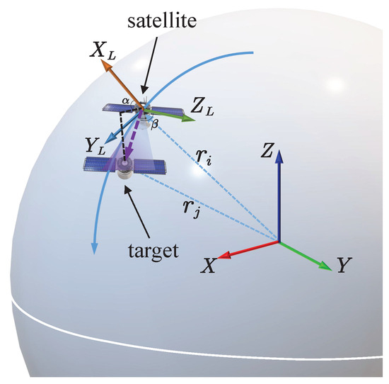
Figure 1.
Schematic diagram of sensor measurement geometry.
The position of the target in satellite j’s LVLH coordinate system is
where is the transformation matrix from the Earth-centered inertial frame to the LVLH coordinate system, and and are the position vectors of target i and observation satellite j, respectively.
2.2.2. Nonlinear Observation Equations
The angle-only observation model of satellite j for target i is
where the measurement function is defined as
The measurement noise , where is the measurement noise covariance matrix.
Figure 1 illustrates the measurement geometry of the satellite sensor. In the LVLH coordinate system, the axis points in the direction of orbital motion, the axis points in the anti-nadir direction (away from Earth’s center), and the axis is determined by the right-hand rule. The satellite sensor obtains angular information of the target by measuring the azimuth angle (the projection angle in the - plane) and the elevation angle (the elevation angle relative to the - plane) of the target’s line of sight (LOS) in this coordinate system. Since angle-only observations from a single satellite can only determine the direction of the target’s line of sight but not the range, at least two satellites are required for cooperative observation to uniquely determine the complete state of the target through triangulation principles.
2.2.3. Measurement Jacobian Matrix
Constructing accuracy metrics requires linearization of the measurement equations. The Jacobian matrix of the measurement function with respect to the target state is
The specific form of this matrix depends on the observation geometry, and its condition number directly affects the observability of the system.
2.3. Accuracy Metric Construction Method
2.3.1. Nonlinear Least Squares Estimation
For the estimation of target trajectory , we employ the nonlinear iterative least squares method (Gauss-Newton), solving the nonlinear estimation problem through iterative linearization. When prior information about the target orbit is known, it is possible to determine which observation conditions will yield higher accuracy orbit estimation results based on the geometric relationship between satellites and targets. Consider the nonlinear system:
By accumulating measurements from multiple time instants and using the known system equations and accumulated measurements, we obtain the estimate of the initial state and its estimation accuracy.
First, perform a Taylor expansion of the measurement equation at the estimate :
Let , substituting yields:
2.3.2. State Transition Matrix
Further considering the relationship between the measurement at time and the initial state :
Expanding at :
Let be the state transition matrix, substituting yields:
Substituting the above equation into and performing Taylor expansion, we obtain the relationship between and :
For convenience of notation, let the measurement matrix at time be , and the state transition matrix from time to time be .
2.3.3. Cumulative Observation Matrix Construction
By extending this to , the relationship between accumulated measurements and state values is as follows:
Considering only the measurement noise yields:
2.3.4. Accuracy Matrix Derivation
Assuming nonlinear iterative least squares can converge near the true value, i.e., , accuracy metrics can be derived by approximately substituting the true value. Define the cumulative observation matrix:
Then, the theoretical accuracy covariance is
where represents the noise standard deviation. The theoretical accuracy covariance is based on linearization analysis at the convergence point, providing a first-order approximation of estimation error. If the noise is not independently and identically distributed, weighting is required according to noise characteristics, which can address process noise effects during weighting.
This accuracy metric provides a theoretical foundation for tracking system performance evaluation. System numerical stability can be assessed through the condition number of cumulative observation matrix ; when the condition number is too large, the estimation process needs to be reinitialized.
2.3.5. Precision Evolution Characteristics and Multi-Target Observation Scheduling
Based on the cumulative observation matrix theoretical framework established by Equation (18), this section analyzes the precision evolution characteristics under stereoscopic observation mode and its guiding effect on multi-target scheduling strategies.
Figure 2 demonstrates the coupling relationship between the positioning precision convergence process of dual-satellite stereoscopic observation and the multi-target cyclic observation scheduling mechanism. The left side describes the precision evolution process of a single target under stereoscopic observation mode, while the right side shows the multi-target resource allocation strategy based on precision states. In the initial stage of stereoscopic observation, target position uncertainty manifests as a large-scale error ellipsoid. Through dual-satellite cooperative angle measurement, combined with the cumulative observation matrix from Equation (17) and the theoretical precision covariance from Equation (18), position error exhibits exponential convergence characteristics. When the condition number of cumulative observation matrix satisfies and the theoretical precision meets mission requirements, the system determines that the target has entered a stable tracking state.
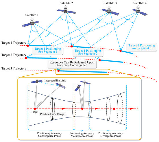
Figure 2.
Stereoscopic observation positioning precision evolution and multi-target cyclic observation mechanism.
Based on the aforementioned precision evaluation mechanism, the multi-target observation scheduling adopts the following strategy: let be the target set and be the satellite set. For any time t, the precision state of target k is defined as
where km is the precision threshold, and km is the transition threshold.
Resource allocation follows the priority principle: targets in divergent state receive stereoscopic observation configuration with at least two satellites for rapid convergence; targets in transitional state maintain single-satellite or dual-satellite observation to prevent precision degradation; targets in convergent state enter low-frequency monitoring mode, releasing resources for other targets to use. This dynamic allocation strategy based on precision metrics ensures global precision optimization under limited observation resource constraints.
2.4. Observability Analysis
The system’s observability directly affects the theoretical limit of tracking precision. For dual-satellite angle measurement observation systems, observability depends on the rank characteristics and condition number of the cumulative observation matrix . As shown in Equation (17), the cumulative observation matrix contains all historical observation information, where m is the number of observing satellites at each moment, and n is the number of observation moments. The necessary condition for complete system observability is
This requires at least 3 moments of dual-satellite observations to uniquely determine the target’s six-dimensional state. However, the rank of the cumulative observation matrix depends not only on the number of observations but more critically on the observation geometric configuration. When the observing satellites, target, and geocenter are approximately coplanar, rank deficiency occurs, leading to the inability to accurately estimate certain state components.
Even when the system is theoretically observable (full rank condition), numerical ill-conditioning can cause severe precision degradation. The condition number of the information matrix is defined as
where and are the maximum and minimum singular values of the cumulative observation matrix, respectively. The condition number quantifies the system’s sensitivity to measurement errors. According to numerical analysis theory, the relative amplification factor of state estimation error is bounded by the condition number:
This means that measurement errors are amplified by the condition number. When , the system is in a weakly observable state, and tracking precision begins to degrade; when , the numerical solution is completely unreliable, and even adding more observation data cannot improve precision.
The theoretical precision covariance based on the cumulative observation matrix directly reflects the quality of system observability. The trace of the precision covariance matrix provides a measure of position error, while its eigenvalue distribution reveals the degree of observability of different state components. When one eigenvalue is much larger than others, it indicates that the corresponding state component has poor observability, requiring adjustment of the observation configuration.
In practical systems, when the condition number exceeds the threshold (e.g., ) or the precision covariance exceeds the tolerance range (e.g., km), observation resource reallocation should be triggered to select satellite combinations that can improve the condition number of the cumulative observation matrix, or to wait for orbital evolution to more favorable relative positions.
3. Hypergraph-Based Optimization Framework
3.1. Hypergraph Modeling and Algebraic Connectivity
3.1.1. Edge-Dependent Vertex-Weighted Hypergraph Definition
According to the work of de Arruda et al. [30], the edge-dependent vertex-weighted (EDVW) hypergraph is defined as a quadruple:
where the following are used:
- is the vertex set, representing satellites.
- is the hyperedge set, representing targets
- is the hyperedge weight function, quantifying the importance of targets.
- is the edge-dependent vertex weight function, where if and only if .
The key innovation of this model lies in allowing vertices (satellites) to have different weights in different hyperedges (targets), accurately capturing the heterogeneity in satellite-target assignments. The weighted degree of a node is defined as
The weighted degree of a hyperedge is defined as
The two-step random walk process defined on the EDVW hypergraph follows the transition probability:
Here, the walker’s transition from vertex to is decomposed into: first selecting a hyperedge e containing with probability , then selecting vertex within hyperedge e with probability .
3.1.2. Laplacian Matrix and Algebraic Connectivity
The normalized Laplacian matrix of the EDVW hypergraph is defined as
where the elements of the weighted adjacency matrix are defined as
The degree matrix is a diagonal matrix with diagonal elements . The Laplacian matrix has properties including positive semi-definiteness (), zero eigenvalue (), and ordered eigenvalues ().
Algebraic connectivity , as the second smallest eigenvalue of the hypergraph Laplacian matrix, quantifies the connectivity strength of the network. According to the spectral gap theorem, is a necessary and sufficient condition for hypergraph connectivity. According to Cheeger’s inequality, algebraic connectivity and the Cheeger constant satisfy the following:
where is the maximum degree, and the Cheeger constant is defined as
High algebraic connectivity provides theoretical guarantees for structural robustness, optimization objective rationality, and numerical stability in multi-target tracking systems.
3.2. Multi-Objective Optimization Problem Modeling
Based on the theoretical framework of precision metrics established in Section 2.3, the satellite-target assignment problem is modeled as a joint precision-robustness optimization problem:
where is the set of satellite pairs assigned to target k.
The robustness metric in the objective function is normalized through algebraic connectivity:
where is the theoretical maximum algebraic connectivity. The precision metric is normalized based on the cumulative observation matrix and theoretical precision covariance:
where the average position error is , , km, km.
Observation constraints include multiple physical and geometric limitations. The limb observation constraint (Equation (34)) requires that the line of sight must be above the Earth’s atmospheric limb height (typically 100–150 km):
where km is the Earth’s radius, and is the satellite orbital altitude.
The sun avoidance constraint (Equation (35)) ensures that the angle between the camera’s line of sight and the sun direction is greater than the avoidance angle to prevent sun damage or interference to the detector:
where is the sun avoidance angle (typically 30–45°).
The detection distance constraint (Equation (36)) limits the effective range of the sensor, with maximum detection distance depending on sensor sensitivity and target intensity:
where NEFD is the noise equivalent flux density, is the atmospheric transmittance, is the target intensity, is the background intensity, and SNR is the signal-to-noise ratio requirement.
The stereoscopic observation angle constraint (Equation (37)) ensures the quality of dual-satellite observation geometry, with constraints set as , , and the stereoscopic observation angle calculated as
The maneuverability constraint (Equation (38)) limits the switching time between consecutive observation tasks, where the maneuver time for a satellite switching from target to target must satisfy:
where and are the azimuth and elevation angle changes, respectively, and and are the maximum angular velocities (typically 1–3°/s).
Based on the EDVW hypergraph model, weight functions are designed to reflect observation quality and precision requirements. The hyperedge weight (target priority) is defined as
where is the target’s base priority, and is the current precision covariance matrix. When precision is poor (large ), the weight increases to obtain more observation resources. The vertex weight (observation contribution) is defined as
where the geometric quality function is .
Based on the theoretical precision framework established in Section 2.3, convergence criteria for target states are defined. When position error km, the target is considered to have converged to a high-precision state, and observation frequency can be reduced or paused. When position error km, intensive observation is needed to restore precision, which typically occurs after target orbital maneuvers, precision divergence due to long periods without observation, or during initial orbit determination phases.
3.3. Constrained Simulated Annealing Optimization Algorithm
For the multi-objective optimization problem defined by Equations (31)–(40), traditional optimization methods face challenges including large problem scale ( binary decision variables, with a search space of ), complex constraints (including multiple coupled constraints such as geometric, observation, and maneuver constraints), conflicting objectives (optimal precision and optimal robustness allocation schemes often differ), and high real-time requirements. Therefore, a constrained simulated annealing (CSA) algorithm is designed to efficiently solve the problem through guided perturbation strategies and adaptive parameter adjustment.
To handle constraints, the penalty function method is adopted to convert constrained optimization into unconstrained optimization. The augmented objective function is defined as
where the penalty term is defined as
Here, denotes the positive part function. Penalty weights are dynamically adjusted based on the current precision state:
where is the theoretical precision covariance based on the cumulative observation matrix, is the average error, is the average capacity, and are base penalty coefficients.
Since the feasible region is very small relative to the search space, relying solely on penalty functions is insufficient to effectively guide the search; thus, two guided perturbation strategies are designed. The first strategy is precision-based directed satellite reallocation, first identifying the set of targets with unsatisfactory precision and the set of insufficiently observed targets , where . Then, identify overloaded and underloaded satellites:
For targets with unsatisfactory precision, satellites from underloaded satellites that can maximally improve the condition number of the cumulative observation matrix are preferentially selected for supplementary allocation.
The second strategy is local satellite exchange based on observation geometry, randomly selecting two targets and checking the feasibility of exchanging their allocated satellites:
where is the cumulative observation matrix after exchange. Strategy selection probability is dynamically adjusted based on the current precision state:
The key innovation of the algorithm lies in deeply integrating the precision metric theory established in Section 2.3 into the optimization process. By computing the theoretical precision covariance matrix for each target in real-time, the algorithm can accurately identify targets requiring focused attention and adjust resource allocation strategies accordingly. Adaptive parameter adjustment strategies include temperature adjustment, perturbation amplitude adjustment, and penalty strength adjustment. Temperature is dynamically adjusted based on acceptance rate:
Penalty strength is dynamically adjusted based on precision satisfaction rate:
where is the set of converged targets.
4. Experimental Design and Methods
4.1. Experimental Scenario Design
The experimental scenario design follows the principle of progressive validation, forming a complete test chain from basic capabilities to extreme performance. This design ensures experimental completeness and progressiveness, with each scenario building upon the previous one, gradually increasing complexity and challenge.
Scenario 1: Baseline Scenario. The baseline scenario provides a performance evaluation under ideal conditions. In this scenario, all targets maintain nominal orbits, all satellites operate normally, with no interference factors. Key performance indicators include steady-state position error should be less than 0.1 km, precision achievement time should be less than 300 s (defined as the time required for position error to drop below 0.05 km), and success rate should exceed 90%. These indicators are set based on actual space surveillance mission requirements.
Scenario 2: Maneuvering Scenario. The maneuvering scenario introduces the key challenge of target maneuvers based on the baseline scenario. In this scenario, 30% of targets will execute random maneuvers with velocity increments between 0.005 and 0.02 km/s, maneuver duration of 30 s, followed by a 300 s cooldown period. Maneuver timing follows a Poisson process with an average occurrence rate of 0.003 per time step. These parameter selections are based on actual space target maneuvering characteristics, covering typical maneuver types such as orbit maintenance, collision avoidance, and orbit adjustment.
Scenario 3: Failure Scenario. The failure scenario is the most stringent test, aimed at verifying the algorithm’s survivability under extreme conditions. In this scenario, satellites fail with a 0.1 probability at each time step, failures lasting 100 to 500 s, with up to 10 satellites (approximately 42%) potentially failing simultaneously. This scenario design is based on an important finding from hypergraph theory: system failure probability has an exponential relationship with algebraic connectivity, and by maximizing algebraic connectivity, failure risk can theoretically be reduced exponentially.
4.2. Comparison Algorithms
To verify the effectiveness of the proposed method, this study compared four allocation algorithms:
Traditional Greedy Algorithm: Based on the geometric proximity principle, selecting the two nearest satellites for observation of each target. This method is computationally simple, with the time complexity of serving as a performance baseline.
CBBA Algorithm: Consensus-Based Bundle Algorithm [36], employing a distributed consensus mechanism, achieving task allocation through two phases: bundle construction and consensus reaching. The algorithm contains two key phases:
- Bundle construction phase: each agent greedily selects tasks based on local information, constructing its own task bundle
- Consensus-reaching phase: agents resolve allocation conflicts through information exchange, achieving global consensus
This algorithm is widely applied in multi-robot systems, with good scalability and robustness.
CSA-Hypergraph Method: The method proposed in this paper (see Section 3) achieves system robustness optimization by maximizing the algebraic connectivity of the EDVW hypergraph. This method models satellite-target allocation as an edge-dependent vertex-weighted hypergraph , where satellites are vertices and targets are hyperedges, enhancing system robustness by optimizing the second smallest eigenvalue of the Laplacian matrix. The specific implementation adopts the constrained simulated annealing framework shown in Algorithm 1, efficiently solving the optimization problem through guided perturbation and adaptive temperature adjustment strategies.
| Algorithm 1 Precision Metric-based Constrained Simulated Annealing Hypergraph Optimization (CSA-Hypergraph). |
|
CSA-Bipartite Graph Method: Converting the hypergraph into an equivalent bipartite graph representation for optimization. Any hypergraph can be naturally represented as a bipartite graph , where the vertex set includes original vertices V (satellites) and hyperedges E (targets), and the edge set connects vertices to the hyperedges containing them. The Laplacian matrix of the bipartite graph is defined as
where is the incidence matrix, when , otherwise 0; and are the degree matrices of satellites and targets, respectively.
While the bipartite graph representation preserves complete information of the hypergraph, there are important differences between the two methods:
- Dimensional difference: The hypergraph Laplacian matrix is dimensional, while the bipartite graph is -dimensional
- Random walk semantics: Random walks on hypergraphs represent indirect connections between satellites (through jointly observing targets), while walks on bipartite graphs alternate between satellites and targets
- Computational complexity: Hypergraph method is , bipartite graph method is
Theoretically, both representations contain the same structural information, but the hypergraph method achieves higher computational efficiency through dimensionality reduction. Within the same computational time, the hypergraph method can execute more iterations, thus more thoroughly exploring the solution space and potentially obtaining better solutions.
4.3. Simulation Environment Configuration
To validate the proposed methods, comprehensive simulations were conducted using the parameters specified in Table 2. The simulation environment was designed to reflect realistic space surveillance scenarios while maintaining computational tractability.
Table 2.
Simulation Parameter Settings.
The Walker constellation configuration (24/3/2) shown in Table 2 was selected to provide global coverage with reasonable redundancy. The 24 satellites are distributed across 3 orbital planes with 2 phase offsets, operating at an altitude of 1600 km with 60° inclination. This configuration ensures that multiple satellites are available for stereoscopic observation at any given time.
The target parameters encompass a representative range of LEO objects, with altitudes spanning from 400 km (typical for some Earth observation satellites) to 1200 km (common for navigation satellites). The inclination range of 30–100° covers both equatorial and polar orbits. The observation parameters, particularly the angular noise of 0.001° and initial position error of 10 km, reflect realistic sensor capabilities and initial orbit determination uncertainties encountered in operational space surveillance systems.
5. Experimental Results and Analysis
This section comprehensively evaluates the performance of the proposed method through three progressive scenarios. Before presenting specific results, this paper first introduces the adaptive observation control mechanism commonly adopted by all algorithms, which is a key component ensuring efficient system operation.
5.1. Adaptive Observation Control Mechanism
The four algorithms in this study all adopt adaptive observation control strategies based on precision metrics, achieving a balance between precision assurance and resource optimization through dynamic resource allocation adjustment.
Figure 3 demonstrates the operational mode of the adaptive observation control mechanism. This mechanism dynamically adjusts observation resource allocation based on the theoretical precision metrics established in Section 2.3, and is a common feature of the four algorithms in this study. The figure uses the CSA-Hypergraph method as an example, selecting 10 representative targets to demonstrate their observation state evolution. Red indicates active observation periods, gray indicates pause periods, and red vertical lines indicate the timing of maneuver events.
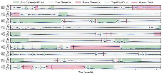
Figure 3.
Example of precision metric-based adaptive observation control mechanism.
The core features of this mechanism include the following:
- 1.
- Precision-driven resource scheduling: When a target’s theoretical precision covariance satisfies km, the system automatically pauses observation of that target, releasing resources for targets whose precision has not yet met standards. This strategy avoids excessive observation of converged targets and improves overall resource utilization efficiency.
- 2.
- Event response mechanism: When target maneuvers are detected, the system automatically resumes observation of that target, ensuring tracking continuity. Maneuver detection is based on statistical testing of batch least squares estimation residuals: when the normalized residual (where m is the measurement dimension and corresponds to 3 confidence), the target is determined to have maneuvered and re-observation is triggered.
This adaptive mechanism enables all algorithms to optimize resource utilization while ensuring tracking precision. Performance differences between algorithms are mainly reflected in the degree of optimization of resource allocation strategies, rather than the adaptive mechanism itself.
The following sections analyze in detail the specific performance of the four algorithms in three test scenarios.
5.2. Scenario 1: Baseline Scenario Results
The baseline scenario provides a baseline reference for algorithm performance evaluation under ideal conditions. In this scenario, all targets maintain nominal orbital motion, the satellite constellation maintains complete operational status, with no external disturbance factors.
Figure 4 shows the average position error evolution characteristics of the four allocation algorithms during the 3600 s simulation period. The CSA-Hypergraph method demonstrates significant performance advantages: its error curve shows a faster descent rate in the initial stage, indicating the algorithm’s superior initial convergence characteristics; in the steady-state phase ( s), the average position error remains stable at 0.089 km level with fluctuation amplitude of only ±0.012 km, demonstrating the algorithm’s numerical stability.
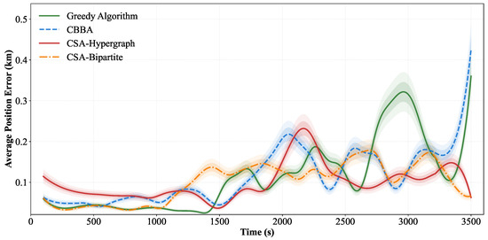
Figure 4.
Average position error evolution curves over time for four methods—baseline scenario.
Figure 5 intuitively presents the spatiotemporal allocation pattern of satellite resources. The horizontal axis represents simulation time, the vertical axis corresponds to 24 Walker constellation satellites, and different color blocks represent time windows when satellites are allocated to specific targets.
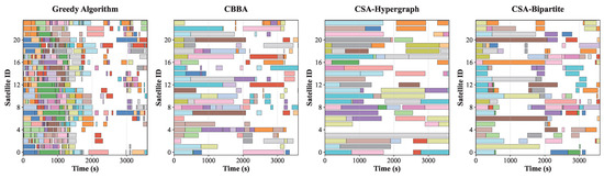
Figure 5.
Gantt chart for four methods—satellite resource allocation timeline.
Figure 6 analyzes resource allocation balance in depth through a heatmap. The figure shows the cumulative usage time of 24 satellites under four methods, with color intensity indicating utilization rate (dark red indicates high utilization, dark blue indicates low utilization).
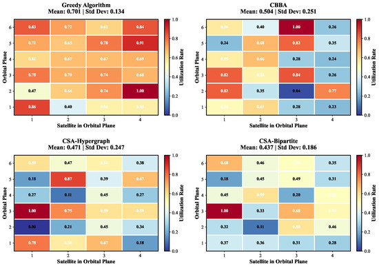
Figure 6.
Satellite resource utilization heatmap.
Table 3 summarizes the performance indicators of the four allocation algorithms in the baseline scenario. The CSA-Hypergraph method achieves the smallest steady-state position error (0.089 km), followed by the CSA-Bipartite Graph method (0.102 km), CBBA (0.124 km), and the Greedy Algorithm (0.152 km). The differences in position errors reflect the optimization objectives of different algorithms: the hypergraph method indirectly optimizes the observation geometric configuration by maximizing algebraic connectivity, thereby achieving higher positioning precision.
Table 3.
Baseline Scenario Performance Indicators.
In terms of precision achievement time, the CSA-Hypergraph method requires only 234.5 s to reduce the initial error (10 km) to high-precision level (below 0.05 km), 44.9% faster than traditional methods. Due to high initial uncertainty, sufficient observations need to be accumulated to achieve the required precision. CBBA requires 356.2 s to complete the precision convergence process.
All algorithms achieve success rates exceeding 90%, with the CSA-Hypergraph method achieving the highest success rate of 98.8%, indicating its ability to reliably satisfy dual-satellite observation constraints (Equation (32)) and satellite resource constraints (Equation (33)) under normal conditions. The differences in success rates mainly stem from algorithms’ strategies in handling resource conflicts: the CSA-Hypergraph method avoids local resource competition through global optimization, while the greedy algorithm may result in some targets being unable to obtain sufficient observation resources due to its first-come-first-serve allocation strategy.
Baseline scenario results indicate that robustness optimization achieved through maximizing hypergraph algebraic connectivity not only improves the system’s fault tolerance but also achieves better observation precision under standard conditions.
5.3. Scenario 2: Maneuvering Scenario Results
The maneuvering scenario evaluates the algorithms’ dynamic adaptation capabilities by introducing target orbital maneuvers. According to the experimental design, 15 targets (30%) randomly execute impulsive orbital maneuvers following a Poisson process (/step), with velocity increments km/s applied instantaneously to targets, with maneuver directions uniformly distributed in three-dimensional space. At least 300 s must pass after each maneuver before another maneuver can be executed.
Table 4 quantitatively shows the key performance differences of the four algorithms in the maneuvering scenario. The CSA-Hypergraph method demonstrates significant advantages in all indicators, validating the effectiveness of algebraic connectivity-based optimization.
Table 4.
Maneuvering Scenario Performance Indicators.
Detection Delay Analysis: The CSA-Hypergraph method achieves the shortest detection delay (28.4 s), 34.3% faster than the greedy algorithm. This advantage stems from the high-quality observation network structure constructed through algebraic connectivity optimization. Specifically, the CSA-Hypergraph method achieves three key advantages by maximizing : First, optimized observation geometric configuration (larger baselines and better intersection angles) increases the information content of single observations, reducing the condition number of the Jacobian matrix , thereby accelerating the convergence of the cumulative observation matrix . Second, the average algebraic connectivity in the maneuvering scenario reaches 0.316 (4.27 times that of the baseline scenario), with high connectivity directly translating to faster information accumulation rates, making residual detection more sensitive to state changes. Third, the optimized network structure ensures numerical stability of batch least squares estimation. In contrast, although the greedy algorithm (43.2 s) and CBBA (38.7 s) also maintain dual-satellite observations, due to a lack of global optimization of observation geometric quality, their cumulative observation matrix converges more slowly, requiring more time to detect abnormal increases in estimation residuals.
Observation Precision Recovery Capability: Re-achievement time reflects the algorithm’s ability to recover good observation precision from maneuver disturbances. The CSA-Hypergraph method requires only 98.7 s to restore position error below 0.05 km, which is 52.6% of the greedy algorithm’s time (187.5 s). This rapid recovery capability benefits from the network structure quality guaranteed by high algebraic connectivity (): First, the optimized network maintains multiple high-quality observation paths, enabling rapid deployment of optimal satellite pairs after maneuvers. Second, continuous high-quality observations ensure smaller initial estimation errors after maneuvers, reducing the number of iterations needed for re-convergence. Third, optimized observation geometry accelerates the improvement of the condition number of the cumulative observation matrix , enabling batch least squares estimation to converge faster to the required precision.
Precision Degradation Control: Precision degradation is defined as the percentage deterioration of tracking precision after maneuvers relative to baseline scenario steady-state precision. The CSA-Hypergraph method controls precision degradation at 43.9%, significantly better than the greedy algorithm’s 86.8%. This result indicates that the observation network constructed through algebraic connectivity optimization not only has higher precision under normal conditions but can also maintain observation performance superior to traditional methods’ baseline levels when facing dynamic disturbances. The CSA-Bipartite Graph method’s precision degradation (52.0%) is slightly higher than the hypergraph method, mainly due to the computational complexity disadvantage of the bipartite graph’s -dimensional representation compared with the hypergraph’s -dimensional representation, limiting optimization sufficiency within the same time constraints.
Figure 7 shows the convergence performance comparison of the four observation scheduling methods. Convergence rate is defined as the proportion of targets whose state estimation error remains below the 0.05 km threshold at the current time. Throughout the entire process, the CSA-Hypergraph and CSA-Bipartite Graph methods outperform the greedy algorithm and CBBA algorithm. The CSA-Hypergraph method (red line) exhibits the most stable convergence characteristics with minimal fluctuation amplitude, possibly because the hypergraph improves system stability through dynamic optimization of algebraic connectivity, enabling the system to maintain stable overall performance while rapidly responding to maneuvers. The CSA-Bipartite Graph method shows significantly slower convergence speed than other methods in the initial phase when s.
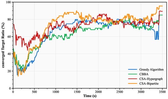
Figure 7.
Comparison of converged target proportions for four methods.
Comprehensive evaluation shows that the CSA-Hypergraph method outperforms CBBA and the greedy algorithm in most time periods, and is comparable to the CSA-Bipartite Graph method but with better stability. This stable and high-quality performance makes the CSA-Hypergraph method more suitable for multi-target observation tasks requiring long-term continuous operation.
5.4. Scenario 3: Failure Scenario Results
The failure scenario simulates system robustness under extreme operating conditions. Satellite failures follow a Bernoulli process (/step), with failure duration following a uniform distribution seconds.
Table 5 quantitatively evaluates the performance of the hypergraph algebraic connectivity-based multi-target tracking system under different failure rates. Performance degradation rate is defined as the percentage increase in average error relative to the baseline scenario.
Table 5.
Performance Degradation and Average Error Comparison Under Different Failure Rates.
From the experimental results, the CSA-Hypergraph method demonstrates good fault tolerance capability, with its degradation rate growing slowly from 3.1% at 10% failure rate to 14.5% at 40% failure rate, presenting an approximately linear stable growth pattern. This stability stems from the hypergraph’s optimization of algebraic connectivity: by optimizing the observation network’s topology and resource allocation efficiency, the system can quickly reconfigure remaining resources when partial nodes fail, reallocating observation tasks originally assigned to failed satellites to nearby available satellites, even sacrificing observation opportunities for some low-priority targets to ensure tracking continuity for critical targets. In contrast, the traditional greedy algorithm and CBBA show degradation rates of 24.3% and 27.2%, respectively, at 40% failure rate, indicating the vulnerability of allocation strategies lacking global optimization under high failure rate conditions.
Second, the CSA-Hypergraph method also performs excellently in absolute precision metrics. Under all failure rate conditions, this method achieves the lowest or second-lowest average error, fully demonstrating the performance maintenance capability of network structures optimized based on algebraic connectivity under extreme conditions.
In sharp contrast to the CSA-Bipartite Graph method’s sharp degradation, the CSA-Hypergraph method’s degradation rate growth remains stable. This stability reflects the inherent advantages of hypergraph representation: by directly modeling the high-order interaction relationships between satellites and targets, the system avoids numerical instability in the bipartite graph’s high-dimensional space. More importantly, the hypergraph’s dimensional representation significantly reduces computational complexity compared with the bipartite graph’s -dimensional representation. This computational efficiency advantage enables more thorough optimization iterations within the same time constraints, thereby obtaining better allocation solutions.
Comprehensive analysis shows that the CSA-Hypergraph method successfully constructs an observation network with inherent robustness through optimizing algebraic connectivity. Even under an extreme 40% failure rate, the system maintains 0.117 km tracking precision, outperforming traditional methods under normal conditions (greedy algorithm baseline precision 0.152 km). This result validates the theoretical prediction: according to Cheeger’s inequality, high algebraic connectivity guarantees the network’s strong connectivity and rapid information diffusion capability, thereby maintaining overall system performance during node failures.
Figure 8 shows the reassignment event statistics for the four algorithms across three scenarios. The greedy algorithm shows significantly higher reassignment frequency than the other three algorithms in all scenarios, reflecting frequent adjustments caused by its local optimization strategy.
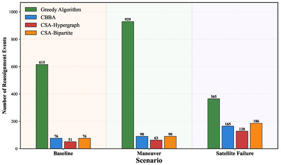
Figure 8.
Reassignment event statistics under different scenarios.
In the maneuvering scenario, the greedy algorithm’s reassignments surge to 929 times, while the CSA-Hypergraph method only increases to 63 times (23.5% increase), maintaining the lowest absolute quantity. This contrast indicates that the CSA-Hypergraph method employs precise local adjustment strategies, avoiding unnecessary reassignments.
In the failure scenario, the greedy algorithm drops to 365 times, because reduced available satellites limit the reassignment selection space, and its simple proximity-based allocation strategy actually reduces adjustment needs when resources are limited. The CSA-Hypergraph method’s absolute quantity remains lower than CBBA and bipartite graph methods, further indicating that the CSA-Hypergraph method can make more precise decisions, reallocating resources only when necessary to maintain multi-target high-precision observation requirements.
5.5. Algebraic Connectivity Analysis
Algebraic connectivity , as the second smallest eigenvalue of the hypergraph Laplacian matrix, quantifies the network’s connectivity strength and information diffusion capability.
Figure 9 shows the temporal evolution characteristics of algebraic connectivity under three test scenarios, with corresponding statistical data shown in Table 6.
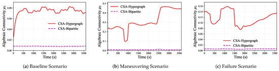
Figure 9.
Evolution curves of under three scenarios.
Table 6.
Algebraic Connectivity Statistics.
In the baseline scenario (Figure 9a), the CSA-Hypergraph method’s average connectivity of 0.074 and standard deviation of 0.028 indicate that the system maintains stable connectivity while preserving moderate adjustment space. This moderate level of algebraic connectivity aligns with the 0.089 km average position error and 234.5 s precision achievement time in Table 3—ensuring the network quality required for high-precision observation while avoiding computational overhead from over-optimization. In contrast, the CSA-Bipartite Graph method’s value remains nearly constant around 0.008 (standard deviation only 0.001), and this excessive stability limits its ability to respond to environmental changes.
In the maneuvering scenario (Figure 9b), the CSA-Hypergraph method’s high algebraic connectivity means that during the initial allocation phase, the selected satellite pairs have better observation geometry, resulting in better condition numbers for the Jacobian matrix in batch least squares estimation, thereby accelerating state estimation convergence. During the next allocation, the algorithm reselects optimal pairs from visible satellites, with alternative options of higher quality due to the optimization of the initial network structure.
In the satellite failure scenario (Figure 9c), the CSA-Hypergraph method’s algebraic connectivity increases by 56.8% compared with the baseline scenario. This may be because, although available nodes decrease, the algorithm reduces the number of tracked targets, concentrating limited resources on high-priority targets; reoptimizes allocation within the constraint space, improving utilization of remaining satellites; and during each reallocation, the algorithm tends to select configurations that maximize network connectivity. Through these methods, better connection patterns are constructed among remaining nodes, resulting in only 9.8% performance degradation at 30% failure rate, significantly outperforming other methods.
6. Conclusions
This paper proposes a hypergraph theory-based optimization framework for multi-target observation systems, validating the method’s effectiveness through theoretical analysis and systematic experiments. This research establishes a theoretical framework for precision metrics based on nonlinear batch least squares estimation, deriving the theoretical precision covariance through the cumulative observation matrix and state transition matrix, providing theoretical guarantees for tracking precision evaluation. The satellite-target allocation problem is modeled as an edge-dependent vertex-weighted hypergraph , enhancing system robustness through maximizing algebraic connectivity , and designing a constrained simulated annealing algorithm to efficiently solve this optimization problem.
Through large-scale simulation experiments of 24 Walker constellation satellites tracking 50 targets, the performance of the CSA-Hypergraph method was comprehensively evaluated in three scenarios, outperforming other algorithms in all cases. In the baseline scenario, this method achieved a steady-state position error of 0.089 km and a precision achievement time of 234.5 s. In the maneuvering scenario, it achieved a detection delay of 28.4 s and a re-achievement time of 98.7 s, controlling precision degradation at 43.9%. In the failure scenario, even facing a 30% satellite failure rate, the system controlled performance degradation at 9.8% through active compensation strategies ( increased to 0.116), maintaining tracking precision at 0.112 km.
Experiments revealed three core advantages of the CSA-Hypergraph method. First, by constructing high-quality initial network configurations, reassignment frequency was significantly reduced (only 51 times in the baseline scenario, 8.3% of the greedy algorithm), reducing system communication overhead. Second, it demonstrated excellent dynamic adaptation capability, maintaining a stable convergence rate of 75–80% throughout the 3600 s simulation, reflecting an optimal balance between rapid response and steady-state maintenance. Third, it possesses inherent fault tolerance capability, maintaining sub-kilometer precision under extreme conditions through network reconfiguration and resource concentration strategies.
Although the CSA-Hypergraph method demonstrates clear advantages, there remains room for improvement. Future work should explore (1) developing incremental update algorithms to reduce computational complexity; (2) introducing machine learning to achieve parameter adaptation. This research provides new theoretical tools and practical methods for space situational awareness system design. By organically combining hypergraph theory, optimization algorithms, and practical constraints, it solves the optimization problem of multi-satellite multi-target observation systems, holding significant importance for enhancing space safety.
Author Contributions
Conceptualization, J.C., X.P., Y.J. and Y.L.; Methodology, J.C. and B.S.; Validation, J.C., B.S. and Y.L.; Investigation, J.C.; Resources, X.P.; Data curation, J.C.; Writing—original draft, J.C.; Writing—review & editing, X.P., Y.J. and B.S.; Visualization, J.C. and Y.L.; Supervision, X.P. and Y.J.; Project administration, B.S.; Funding acquisition, X.P., Y.J. and B.S. All authors have read and agreed to the published version of the manuscript.
Funding
This research was funded by the National Natural Science Foundation of China (No. 62503487), National University of Defense Technology Scientific Research Fund for Young Scholars’ Independent Innovation (No. ZK25-60), the National University of Defense Technology Independent Innovation Research Fund (No. 24-ZZCX-GZZ-01-01), the National Key Laboratory of Space Intelligent Control (No. 2024-CXPT-GF-JJ-012-16), and National Key Laboratory of Spacecraft Thermal Control Open Fund (No. NKLST-JJ-005).
Data Availability Statement
The original contributions of this research are contained in the article. For further inquiries, please contact the corresponding author.
Conflicts of Interest
The authors declare no conflicts of interest.
References
- Massimi, F.; Ferrara, P.; Petrucci, R.; Benedetto, F. Deep Learning-based Space Debris Detection for Space Situational Awareness: A Feasibility Study Applied to the Radar Processing. IET Radar Sonar Navig. 2024, 18, 635–648. [Google Scholar] [CrossRef]
- Zhao, P.; Liu, J.; Wu, C. Survey on Research and Development of On-Orbit Active Debris Removal Methods. Sci. China Technol. Sci. 2020, 63, 2188–2210. [Google Scholar] [CrossRef]
- Jia, Q.; Xiao, J.; Bai, L.; Zhang, Y.; Zhang, R.; Feroskhan, M. Space Situational Awareness Systems: Bridging Traditional Methods and Artificial Intelligence. Acta Astronaut. 2025, 228, 321–330. [Google Scholar] [CrossRef]
- Montaruli, M.F.; Purpura, G.; Cipollone, R.; Vittori, A.D.; Facchini, L.; Di Lizia, P.; Massari, M.; Peroni, M.; Panico, A.; Cecchini, A.; et al. An Orbit Determination Software Suite for Space Surveillance and Tracking Applications. CEAS Space J. 2024, 16, 619–633. [Google Scholar] [CrossRef]
- Zhang, Z.; Zhang, G.; Cao, J.; Li, C.; Chen, W.; Ning, X.; Wang, Z. Overview on Space-Based Optical Orbit Determination Method Employed for Space Situational Awareness: From Theory to Application. Photonics 2024, 11, 610. [Google Scholar] [CrossRef]
- Sciré, G.; Santoni, F.; Piergentili, F. Analysis of Orbit Determination for Space Based Optical Space Surveillance System. Adv. Space Res. 2015, 56, 421–428. [Google Scholar] [CrossRef]
- Feng, Z.; Yan, C.; Qiao, Y.; Xu, A.; Wang, H. Effect of Observation Geometry on Short-Arc Angles-Only Initial Orbit Determination. Appl. Sci. 2022, 12, 6966. [Google Scholar] [CrossRef]
- Hu, Y.; Li, K.; Liang, Y.; Chen, L. Review on Strategies of Space-Based Optical Space Situational Awareness. J. Syst. Eng. Electron. 2021, 32, 1152–1166. [Google Scholar] [CrossRef]
- Zisk, R. The Proliferated Warfighter Space Architecture (PWSA): An Explainer. Available online: https://payloadspace.com/ndsa-explainer/ (accessed on 24 September 2025).
- Han, Y.; Wang, L.; Fu, W.; Zhou, H.; Li, T.; Xu, B.; Chen, R. LEO Navigation Augmentation Constellation Design with the Multi-Objective Optimization Approaches. Chin. J. Aeronaut. 2021, 34, 265–278. [Google Scholar] [CrossRef]
- Gerkey, B.P.; Matarić, M.J. A Formal Analysis and Taxonomy of Task Allocation in Multi-Robot Systems. Int. J. Robot. Res. 2004, 23, 939–954. [Google Scholar] [CrossRef]
- Korsah, G.A.; Stentz, A.; Dias, M.B. A Comprehensive Taxonomy for Multi-Robot Task Allocation. Int. J. Robot. Res. 2013, 32, 1495–1512. [Google Scholar] [CrossRef]
- Wang, Q.; Chen, X.; Qi, Q.; Li, M.; Gerstacker, W. Multiple-Satellite Cooperative Information Communication and Location Sensing in LEO Satellite Constellations. IEEE Trans. Wirel. Commun. 2025, 24, 3346–3361. [Google Scholar] [CrossRef]
- Chen, P.; Mao, X.; Chen, S. LEO Satellite Navigation Based on Optical Measurements of a Cooperative Constellation. Aerospace 2023, 10, 431. [Google Scholar] [CrossRef]
- Shen, K.; Yuan, W.; Yan, J.; Ma, K. MCST: An Adaptive Tracking Algorithm for High-Speed and Highly Maneuverable Targets Based on Bidirectional LSTM Network. IEEE Trans. Aerosp. Electron. Syst. 2025, 61, 3205–3226. [Google Scholar] [CrossRef]
- Rong Li, X.; Jilkov, V.P. Survey of Maneuvering Target tracking. Part I: Dynamic Models. IEEE Trans. Aerosp. Electron. Syst. 2003, 39, 1333–1364. [Google Scholar] [CrossRef]
- Chong, C.-Y. Tracking and Data Fusion: A Handbook of Algorithms (Bar-Shalom, Y. et al; 2011) [Bookshelf]. IEEE Control Syst. 2012, 32, 114–116. [Google Scholar]
- Van Trees, H.L. Detection, Estimation, and Modulation Theory; Wiley: New York, NY, USA, 1968. [Google Scholar]
- Guo, J.; Tao, H. Cramer-Rao Lower Bounds of Target Positioning Estimate in Netted Radar System. Digit. Signal Process. 2021, 118, 103222. [Google Scholar] [CrossRef]
- Tasif, T.H.; Hippelheuser, J.E.; Elgohary, T.A. Analytic Continuation Extended Kalman Filter Framework for Perturbed Orbit Estimation Using a Network of Space-Based Observers with Angles-Only Measurements. Astrodyn 2022, 6, 161–187. [Google Scholar] [CrossRef]
- Hue, C.; Le Cadre, J.-P.; Perez, P. Posterior Cramer-Rao Bounds for Multi-Target Tracking. IEEE Trans. Aerosp. Electron. Syst. 2006, 42, 37–49. [Google Scholar] [CrossRef]
- Rashid, M.; Dansereau, R.M. Cramér–Rao Lower Bound Derivation and Performance Analysis for Space-Based SAR GMTI. IEEE Trans. Geosci. Remote Sens. 2017, 55, 6031–6043. [Google Scholar] [CrossRef]
- Walker, J. Continuous Whole-Earth Coverage by Circular-Orbit Satellite Patterns; Technical Report 77044; Royal Aircraft Establishment: Farnborough, UK, 1977. [Google Scholar]
- Guan, M.; Xu, T.; Gao, F.; Nie, W.; Yang, H. Optimal Walker Constellation Design of LEO-Based Global Navigation and Augmentation System. Remote Sens. 2020, 12, 1845. [Google Scholar] [CrossRef]
- Fiedler, M. Algebraic Connectivity of Graphs. Czech. Math. J. 1973, 23, 298–305. [Google Scholar] [CrossRef]
- Jamakovic, A.; Van Mieghem, P. On the Robustness of Complex Networks by Using the Algebraic Connectivity; Lecture Notes in Computer Science; Springer: Berlin/Heidelberg, Germany, 2008; pp. 183–194. [Google Scholar]
- Xu, X.; Gao, Z.; Liu, A. Robustness of Satellite Constellation Networks. Comput. Commun. 2023, 210, 130–137. [Google Scholar] [CrossRef]
- Battiston, F.; Cencetti, G.; Iacopini, I.; Latora, V.; Lucas, M.; Patania, A.; Young, J.-G.; Petri, G. Networks beyond Pairwise Interactions: Structure and Dynamics. Phys. Rep. 2020, 874, 1–92. [Google Scholar] [CrossRef]
- Boccaletti, S.; De Lellis, P.; del Genio, C.I.; Alfaro-Bittner, K.; Criado, R.; Jalan, S.; Romance, M. The Structure and Dynamics of Networks with Higher Order Interactions. Phys. Rep. 2023, 1018, 1–64. [Google Scholar] [CrossRef]
- De Arruda, G.F.; He, W.; Heydaribeni, N.; Javidi, T.; Moreno, Y.; Eliassi-Rad, T. Assigning Entities to Teams as a Hypergraph Discovery Problem. arXiv 2024, arXiv:2403.04063. [Google Scholar] [CrossRef]
- Gu, J.; Feng, S.; Wei, Y. Hypergraph Analysis Based on a Compatible Tensor Product Structure. Linear Algebra Its Appl. 2024, 682, 122–151. [Google Scholar] [CrossRef]
- Cui, C.; Luo, Z.; Qi, L.; Yan, H. The Analytic Connectivity in Uniform Hypergraphs: Properties and Computation. Numer. Linear Algebra Appl. 2023, 30, e2468. [Google Scholar] [CrossRef]
- Young, J.-G.; Petri, G.; Peixoto, T.P. Hypergraph Reconstruction from Network Data. Commun. Phys. 2021, 4, 135. [Google Scholar] [CrossRef]
- Heydaribeni, N.; Zhan, X.; Zhang, R.; Eliassi-Rad, T.; Koushanfar, F. Distributed Constrained Combinatorial Optimization Leveraging Hypergraph Neural Networks. Nat. Mach. Intell. 2024, 6, 664–672. [Google Scholar] [CrossRef]
- Choi, H.-L.; Brunet, L.; How, J.P. Consensus-Based Decentralized Auctions for Robust Task Allocation. IEEE Trans. Robot. 2009, 25, 912–926. [Google Scholar] [CrossRef]
- Chen, J.; Qing, X.; Ye, F.; Xiao, K.; You, K.; Sun, Q. Consensus-Based Bundle Algorithm with Local Replanning for Heterogeneous Multi-UAV System in the Time-Sensitive and Dynamic Environment. J. Supercomput. 2022, 78, 1712–1740. [Google Scholar] [CrossRef]
- Smith, D.; Wetherall, J.; Woodhead, S.; Adekunle, A. A Cluster-Based Approach to Consensus Based Distributed Task Allocation. In Proceedings of the 2014 22nd Euromicro International Conference on Parallel, Distributed, and Network-Based Processing, Turin, Italy, 12–14 February 2014; pp. 428–431. [Google Scholar]
- Arroyo Cebeira, A.; Asensio Vicente, M. Adaptive IMM-UKF for Airborne Tracking. Aerospace 2023, 10, 698. [Google Scholar] [CrossRef]
- Li, J.; Liang, X.; Yuan, S.; Li, H.; Gao, C. A Strong Maneuvering Target-Tracking Filtering Based on Intelligent Algorithm. Int. J. Aerosp. Eng. 2024, 2024, 9981332. [Google Scholar] [CrossRef]
- Lu, W.; Gao, W.; Liu, B.; Niu, W.; Peng, X.; Yang, Z.; Song, Y. Parallel Dual Adaptive Genetic Algorithm: A Method for Satellite Constellation Task Assignment in Time-Sensitive Target Tracking. Adv. Space Res. 2024, 74, 5192–5213. [Google Scholar] [CrossRef]
- Liu, Y.; Wen, Z.; Zhang, S.; Hu, H. Learning-Based Constellation Scheduling for Time-Sensitive Space Multi-Target Collaborative Observation. Adv. Space Res. 2024, 73, 4751–4766. [Google Scholar] [CrossRef]
- Li, S.; Zhang, C.; Zhao, C.; Xia, C. Analyzing the Robustness of LEO Satellite Networks Based on Two Different Attacks and Load Distribution Methods. Chaos Interdiscip. J. Nonlinear Sci. 2024, 34, 033123. [Google Scholar] [CrossRef]
- Chu, K.; Cheng, S.; Zhu, L. A Robust Routing Strategy Based on Deep Reinforcement Learning for Mega Satellite Constellations. Electron. Lett. 2023, 59, e12820. [Google Scholar] [CrossRef]
- Battiston, F.; Amico, E.; Barrat, A.; Bianconi, G.; Ferraz de Arruda, G.; Franceschiello, B.; Iacopini, I.; Kéfi, S.; Latora, V.; Moreno, Y.; et al. The Physics of Higher-Order Interactions in Complex Systems. Nat. Phys. 2021, 17, 1093–1098. [Google Scholar] [CrossRef]
- Vallado, D.A. Fundamentals of Astrodynamics and Applications; McGraw-Hill: New York, NY, USA, 1997. [Google Scholar]


Disclaimer/Publisher’s Note: The statements, opinions and data contained in all publications are solely those of the individual author(s) and contributor(s) and not of MDPI and/or the editor(s). MDPI and/or the editor(s) disclaim responsibility for any injury to people or property resulting from any ideas, methods, instructions or products referred to in the content. |
© 2025 by the authors. Licensee MDPI, Basel, Switzerland. This article is an open access article distributed under the terms and conditions of the Creative Commons Attribution (CC BY) license (https://creativecommons.org/licenses/by/4.0/).