Dynamic Equivalence of Active Distribution Network: Multiscale and Multimodal Fusion Deep Learning Method with Automatic Parameter Tuning

Abstract

Dynamic equivalence of active distribution networks (ADNs) is emerging as one of the most important issues for the backbone network security analysis due to high penetration of distributed generations (DGs) and electricity vehicles (EVs). The multiscale and multimodal fusion deep learning (MMFDL) method proposed in this paper contains two modalities, one of which is a CNN + attention module to simulate Newton Raphson power flow calculation (NRPFC) for the important feature extraction of a power system caused by disturbance, which is motivated by the similarities between NRPFC and convolution network computation. The other is a long short-term memory (LSTM) + fully connected (FC) module for load modeling based on the fact that LSTM + FC can represent a load′s differential algebraic equations (DAEs). Moreover, to better capture the relationship between voltage and power, the multiscale fusion method is used to aggregate load modeling models with different voltage input sizes and combined with CNN + attention, merging as MMFDL to represent the dynamic behaviors of ADNs. Then, the Kepler optimization algorithm (KOA) is applied to automatically tune the adjustable parameters of MMFLD (called KOA-MMFDL), especially the LSTM and FC hidden layer number, as they are important for load modeling and there is no human knowledge to set these parameters. The performance of the proposed method was evaluated by employing different electric power systems and various disturbance scenarios. The error analysis shows that the proposed method can accurately represent the dynamic response of ADNs. In addition, comparative experiments verified that the proposed method is more robust and generalizable than other advanced non-mechanism methods.

1. Introduction

Dynamic equivalence of active distribution networks (ADNs) is an significant aspect of power system protection, planning and operation [1,2]. With the high penetration of renewable energy, plug-in electric vehicles (EVs) as well as energy storage, changed from being a passive one to being an active one. Consequently, the power interaction between the ADNs and the backbone network has become more complicated, which poses a great challenge to the power system operation and security analysis.

During the past few decades, much of the literature has shown that if an equivalent model cannot accurately reflect the dynamic behaviors of the ADNs, an inverse conclusion is drawn in voltage stability assessments and dynamic security analyses of power system [3,4], especially in time-varying and stochastic environments. There have been painful cases, such as the one that occurred in 1996: Western Electricity Coordinating Council (WECC) power outage [5]. Moreover, it can be difficult to track the dynamic characteristics of these complex distribution networks using traditional equivalent method. Therefore, how to formulate an accurate and robust ADN equivalence model is an important issue in power system studies.

The dynamic equivalent of ADNs contains two parts: (1) Determining the structure of the equivalent model. (2) Identifying the parameters of the equivalent model. Load modeling is one important part for deciding upon the equivalent model of ANDs. Nowadays, load modeling methods can be generally divided into three categories: measurement-based methods, component-based methods and fault simulation methods. The basic idea of the component-based approach [6,7,8,9] is to consider the load as a collection of individual users: first the electrical appliances of these users are categorized, and the average characteristics of the various types of electrical appliances are determined; then the proportions of the various appliances are calculated; and finally, the overall load model is synthesized. Nevertheless, this method is heavily dependent on the accurate load composition information. Thus, the method is time-consuming and laborious; additionally, the time-varying load means that this process cannot be carried out online. The measurement-based method [10,11,12,13,14] considers the load as a whole: First, the structure of the load model is determined; Then the field data is collected from the measurement device; Finally the parameters of the load model are identified by employing an optimization algorithm and field data. Compared with the component-based method, the measurement-based method is widely used for representing dynamic behaviors of ADNs due to the load time-variant characteristics. The fault simulation method is actually a test method, and it is difficult to ensure that the load parameters for some faults are applicable to other faults. In addition, the idea that the load parameters are uniformly the same and constant throughout the system is clearly not in line with the essence of loads.

Once the structure of the equivalence model is determined, the equivalence problem transforms into a parameter identification problem. Traditional parameter identification methods include mathematical optimization techniques and modern evolutionary algorithms. Mathematical approaches [15,16], such as least squares and steepest descent, offer fast convergence and reliable solutions. However, they are prone to getting trapped in local optima, especially when the initial values are far from the actual ones. On the other hand, modern evolutionary algorithms [17] suffer from poor robustness, slow convergence, and difficulties in parameter tuning. Moreover, due to the real-time requirements of online parameter identification for equivalent models, evolutionary algorithms—often involving numerous strategies and parameters—tend to be computationally intensive, making them unsuitable for time-varying load conditions. To meet real-time constraints, mathematical methods typically rely on simplified models [16], which can compromise identification accuracy. Deep learning-based equivalent methods are typical non-mechanistic models. Although their parameters lack clear physical meaning and may be less intuitive to engineers, they offer superior capability in capturing dynamic characteristics compared to traditional methods. Once trained, deep networks can perform parameter identification (i.e., inference) very rapidly, although the training process itself is time-consuming. Overall, compared to mathematical methods, deep learning approaches provide a better balance between accuracy and the demands of online equivalence.

Recently, deep learning (i.e., convolutional NNs (CNNs), and recurrent NNs (RNNs)) has been widely applied in various field for classification and regression. In order to address the load modeling problem, researchers have proposed many neural networks (NNs) methods to track the dynamic behaviors of ADNs, in which consider voltage and frequency as inputs of NNs and finding the mapping relationship to output the real power and reactive power [18,19,20,21,22,23]. Reference [18] points out that the feed forward NNs can prescribe the load modeling function, and the real data collected from Taiwan power company are used to evaluate the performance of the model. In reference [19], M. Bostanci et al. investigated a feedback connection-based NNs dynamic load identification technique, and employed delayed inputs to output real and reactive response. Chen et al. [20] proposed a NNs model to analyze the voltage stability in order to make results more credible considering load dynamic characteristic. Moreover, reference [21] combined the radial basis function NN and the lookup table to track the dynamic response of electrical arc furnace (EAF). However, the cases with more distributed generations (DGs) and electric vehicles (EVs) in ADNs have not been taken into consideration. Besides, the above proposed ANN without temporal connection causing they can not capture the disturbance long term impact (i.e., disturbance occurring at time t will affect the power response of the power system at time t + $\tau$), and further degrade the performance of the model.

RNNs possess a natural dynamic architecture: their self-connected hidden units retain past information and explicitly model temporal dependencies. Consequently, RNNs have proven effective in reproducing the dynamic behavior of active distribution networks (ADNs) [22,23]. In [22], Zheng et al. used an RNN to build a measurement-driven equivalent that accurately tracked ADN dynamics; Test results demonstrated that the RNN surrogate can replace the full network without noticeable loss of fidelity. Traditional RNNs, however, suffer from vanishing or exploding gradients when the sequence length increases, which limits their ability to capture long-range time dependencies. Gated variants—Long Short-Term Memory (LSTM) and Gated Recurrent Units (GRU)—overcome this drawback by selectively storing and updating internal states. Exploiting the formal similarity between the LSTM forward pass and the differential-algebraic equations that govern dynamic loads, ref. [23] proposed an LSTM-based equivalent for ADN dynamic response. PSCAD simulations verified the high accuracy of the resulting model.

It is worth noting that there are three main issues that have not been focused on in the above dynamic equivalence references. The first issue is that the time-variant network parameters of power system caused by disturbance has not been taken into consideration. For example, in IEEE 9-bus transmission network and IEEE 33-bus distribution network system, when three-phase short-circuit disturbance occurs between line 2 and line 3 in distribution network, the loads, nodes and lines connected to line 3 of distribution network would be cut off, so that the entire system topology will change to a system containing an IEEE 9-bus transmission network and a changed distribution network including the nodes of 4, 17, 18, 19, 20, fault resistance connected to node 16 and related lines. When the disturbance is removed from the distribution location, the system topology structure is reverts to its pre-disturbance state. This dynamic process is the reason why the response of ADNs change greatly during the disturbance period. However, conventional non-mechanism equivalent method often overlooked this essence and consider only simple input characteristics to find the mapping between voltage/frequency and active/reactive power. Conventional “non-mechanistic” equivalents ignore this switching behavior: they treat the network as a fixed map from voltage/frequency to active/reactive power and therefore cannot track the moment the graph itself changes. Compounding the problem, the literature has not systematically examined how the equivalent should adapt to different disturbance types, locations or the distinct post-disturbance topologies they create.

The second problem is the choice of voltage-input step size when an LSTM is used for ADN dynamic equivalence. Reference [23] claims that accuracy saturates once the step length passes an empirical “knee point,” yet offers no experimental evidence. Our own comprehensive tests contradict this assertion: within a realistic range the active- and reactive-power errors show no monotonic trend with step size; instead they fluctuate randomly. Only when the step grows beyond a dataset-dependent threshold does the error begin to rise systematically. Consequently, the presumed knee-point rule cannot be relied upon and the step must be treated as a case-specific hyper-parameter.

In deep learning (DL), the adjustable parameter settings (i.e., learning rate, mini-batch size and hidden unite number) largely affect its performance, while selecting appropriate parameters is a demanding and burdensome task. Therefore, the third issues is that the above literature do not consider this problem [18,19,20,21] or applied trial-and-error method to only determine the numbers of RNN + FC layer [22,23]. Moreover, many references about tuning parameters of DL rarely optimized neural network layers, but for the problem of dynamic equivalence using LSTM + FC stacked NNs, determining their depth is crucial. This is because LSTM and FC theoretically represent dynamic and static loads. When there are many dynamic loads in the distribution network, the number of LSTM layers should also increase, and vice versa. The same conclusion also applies to FC. In practice, it is often not possible to find suitable parameters through trial and error methods, as manual testing requires considerable expertise in the DL and the problem domain under consideration. This barrier may prevent the application of MMFDL in dynamic equivalent of ADNs. Recently, metaheuristic search approaches provided an effective way to optimize the parameters of the DL, such as genetic algorithm (GA) and differential evolution (DE). The Kepler Optimization Algorithm (KOA) is a novel physics based metaheuristic algorithm inspired by Kepler′s laws of planetary motion [24,25]. It is worth mentioning that no attention has been paid to automatic parameter optimization (especially the depth of the LSTM + FC NNs in MMFDL) of MMFDL based on KOA for dynamic equivalent of ADNs.

Overall, the main differences between this paper and existing research are summarized as follows: (a) motivated by the similarities between corrected node voltage equation of Newton Raphson power flow calculation (NRPFC) and convolution computation of convolutional neural network (CNN), we employ CNN + attention module to simulate the corrected node voltage equation to extract import features caused by disturbance. (b) The LSTM + FC module is also employed for load modeling. However, different from the previous methods, we employ multiscale fusion method to aggregate the load modeling models with different voltage input size to better capture the relationship between voltage inputs and power outputs, and then combined with CNN + attention module to merge as multiscale and multimodal fusion deep learning (MMFDL) dynamic equivalent method for better tracking dynamic behaviors of ADNs under various disturbance conditions. (c) To eliminate the labor-intensive manual tuning required in [22,23], we cast the MMFDL parameters (especially the depth of the LSTM and FC layers) as an optimisation problem and solve it automatically with the Kepler Optimisation Algorithm (KOA). Furthermore, no attention has been paid to dealing with the problem in parameters optimization of MMFDL based on KOA for dynamic equivalent problem. Our research work is a novel attempt to use KOA-based MMFDL equivalent method in dynamic equivalent of ADNs.

The key contributions of this article are listed as follows:

(1) Motivated by the similarities between corrected node voltage equation of Newton Raphson power flow calculation (NRPFC) and convolution computation of CNN, the CNN + attention module is applied for extracting the important features caused by the disturbance.

(2) To better capture the relationship between voltage and power outputs in load modeling modules, we adopt a multiscale fusion method to aggregate load modeling models with different voltage input size.

(3) The CNN + attention module combined with the load modeling module serves as a multiscale and multimodal fusion deep learning method for representing the dynamic behaviors of ADNs.

(4) The KOA algorithm ia adopted to automatically tune the adjustable parameters of MMFDL, especially the depth of LSTM and FC layers, to overcome the weakness of lacking extensive domain expertise.

The remainder of this paper is organized as follows. Section 2 introduces some important concepts of LSTM, CNN and self attention (SFA) mechanism. Besides, the motivations of adopting multiscale and multimodal deep learning are explained, and the framework of KOA-based MMFDL equivalent method are also designed. In Section 3, the KOA-based automatic parameters tuning method for MMFDL is discussed. Then, Section 4 is about study cases of the KOA-MMFDL equivalent model. Finally, conclusion is drawn in Section 5.

2. A Multiscale and Multimodal Deep Learning (MMFDL) Method

The proposed KOA-MMFDL method contains two parts including MMFDL and KOA, as shown in Figure 1. Therefore, in this section, we first introduced the concepts of some important elements in MMFDL, such as self attention (SFA) mechanism and the block of LSTM and CNN. Then, the reason of why choosing MMFDL equivalence method for tracking dynamic behaviors of ADNs is explained. Finally the basic principle and guidelines of MMFDL equivalent model are introduced.

2.1. Long Short-Term Memory (LSTM)

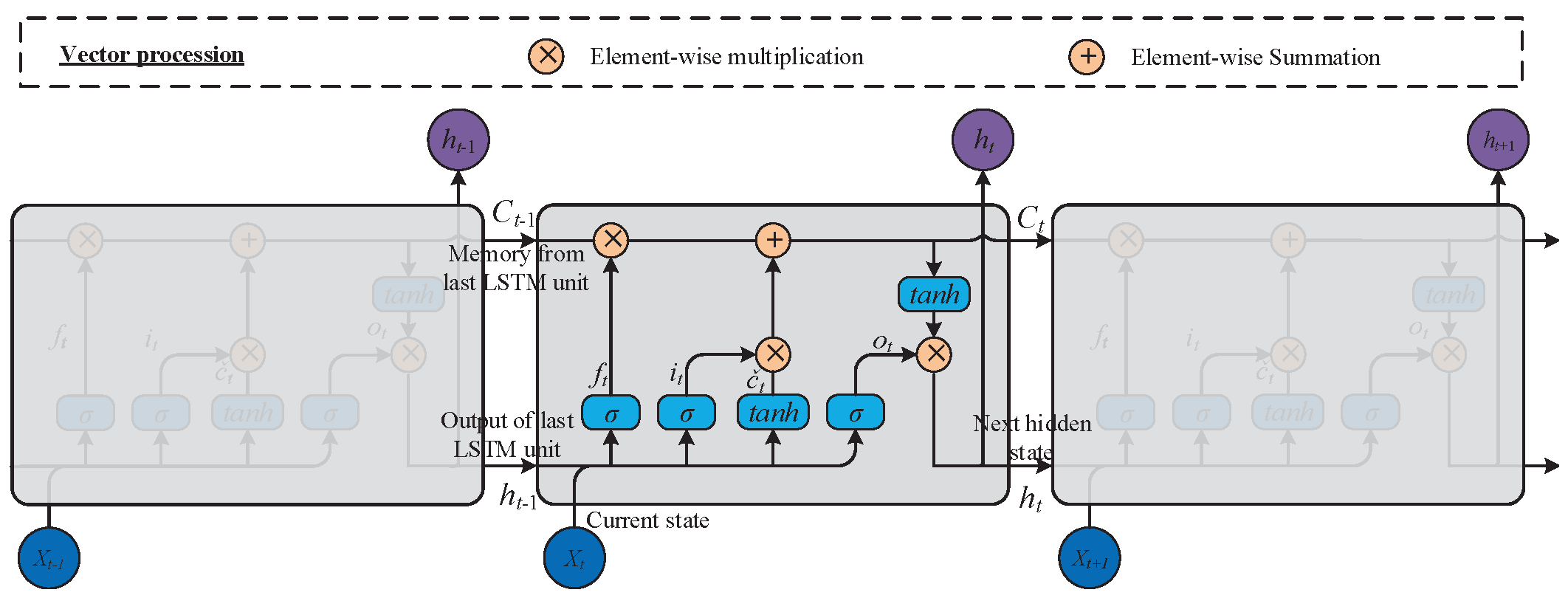
As mentioned in introduction, RNNs suffer from gradient vanishing and exploding issues, making it difficult for then to solve long-term dependencies [26]. In order to break this limitation, German researchers S. Hochreiter and J. Schmidhuber designed an advanced recursive neuron structure based on gates, called LSTM [27]. The architecture of LSTM is shown in Figure 2.

The LSTM contains three gates with different functions, namely input gate, forget gate and output gate, and one memory cell. Memory units form the core of LSTM, responsible for maintaining and updating long-term dependency information throughout the sequence processing. The purpose of the forget gate is to determine which information should be forgotten or retained from the memory unit at each time step. The formulations of an LSTM network are expressed as follows:

$$f_t=\sigma \left(w_{fh}{h}_{t-1}+w_{fx}{X}_t+b_f\right)$$

(1)

$$i_t=\sigma \left(w_{ih}{h}_{t-1}+w_{ix}{X}_t+b_i\right)$$

(2)

$${\check{C}}_t=tanh\left(w_{ch}{h}_t+w_{cx}{X}_t+b_c\right)$$

(3)

$$C_t=f_t\otimes C_{t-1}+i_t\otimes {\check{C}}_t$$

(4)

$$o_t=\sigma \left(w_{oh}{h}_{t-1}+w_{ox}{X}_t+b_o\right)$$

(5)

$$h_t=o_t\otimes tanh\left(C_t\right)$$

(6)

where $f_t$, $i_t$ and $o_t$ are the activation values of the forget gate, input gate, and output gate, respectively. ${\check{C}}_t$ is a candidate memory cell, $\sigma$ is the sigmoid activation function. The meanings of other marks can be found in reference [23].

2.2. Convolutional Computation of CNN

The CNN is known by its strong feature extraction ability, and achieves great success in many fields in recent years. The convolutional layer is the core component of CNN. It can reduce the number of parameters and network complexity of CNN, and extract the characteristics of the input data by convolutional computation. The formulation of convolutional layer can be expressed as:

$$\begin{array}{cc}\hfill s(i,j)& =(X\ast W)(i,j)+b\hfill \\ & =\sum _m\sum _{n}x(i+m,j+n)w(m,n)+\sum _m{b}_m\hfill \end{array}$$

(7)

where X is the input matrix, W and b denote the weights matrix and bias vector of the feature map kernel, respectively.

2.3. Self Attention Model

Generally, the reactive power can not be transmitted over long distances. Therefore, the voltage distribution in power systems remains localized following disturbances, with different disturbance characteristics exerting varying effects on the output response of boundary nodes. Consequently, the response of boundary nodes is contingent upon the operational conditions generated by the disturbance, necessitating attention mechanisms to extract critical features such as adjacent lines and equipment. The self attention mechanism is mainly used to process sequential data, which can calculate attention weights at different positions at different time steps, thereby integrating and interacting information from all time steps. The input of CNN in this article is also time series data, so self attention mechanism is used to extract important features of power grid topology changes.

The principle of self attention mechanism is to calculate the attention weight based on the relationship between the query, key, and value, and then multiply the weight with the value to obtain the weighted sum of each time step, thus obtaining the final output result. Assuming $x_i$ represents the i th element of the $X=\left[x_1, x_2, \dots , x_n\right]$ sequence. Calculate the query (Q), key (K), and value (V) for each element $x_i$ separately.

$$\left\{Q,K,V\right\}=\left\{W^Q,W^K,W^V\right\}\ast x_i$$

(8)

where $W^Q$, $W^K$ and $W^V$ are weight matrix of Q, K and V, respectively. Then perform dot product operation on Query and Key to calculate attention weight:

$$attn=softmax\left(Q\ast K^T/\sqrt{\left(d_K\right)}\right)$$

(9)

Finally, the attention weights are weighted and summed with the values to obtain the output of the model:

$$ou{t}_i=\sum _{j=1}^n\left(att{n}_i\ast V_j\right)$$

(10)

2.4. Reason of Choosing Multiscale and Multimodal Machine Learning for ADNs Equivalence

The long and short influence caused by disturbance in power system response can be captured by LSTM, thanks to LSTM structure with long-short term dependencies extraction ability. It has been approved that LSTM + FC can represent the DAEs of the loads, that is the AEs (Equation (12)) and discrete version of DEs (Equation (11)) are similar to forward calculation procedure of FC (Equation (14)) and LSTM (Equation (13)), respectively.

$$x\left(t\right)=f^{\prime }(x(t-1),u\left(t\right),p)$$

(11)

$$y\left(t\right)=g\left(x\right(t),u(t),p)$$

(12)

$$h\left(t\right)=F\left(h(t-1),v\left(t\right),W_l,b_l\right)$$

(13)

$$O\left(t\right)=G\left(h\left(t\right),v\left(t\right),W_f,b_f\right)$$

(14)

where x, y, u and p denote the state vector, output vector, input vector and parameter vector, respectively. $h\left(t\right)$ and $O\left(t\right)$ indicate hidden state of LSTM and output of FC, respectively. $W_l, W_f$, and $b_l, b_f$ are their weight matrix and bias vector.

Another reason for MMFDL equivalence method is that the response of boundary bus can be obtained by NRPFC. The Newton-Raphson method for power flow calculation computes power correction values through matrix multiplication of the Jacobian matrix and the state error vector, then iteratively refines the power values. When the state error falls below a preset threshold, convergence is achieved. This iterative approach aligns with neural networks in minimizing loss values and propagating losses backward during training. Additionally, the convolution operations in two-dimensional convolutional networks can be transformed into standard matrix-vector multiplication operations, as convolution is fundamentally a specialized form of matrix multiplication. The convolution kernels in convolutional networks can be represented as vectors, and the Jacobian matrix from power systems can serve as input to CNNs.

According to power system network equation, the power flow calculation process of NRPFC can be summarized as follows.

The power flow equation of the i th node is:

$$\left(e_i+\mathrm{j}{f}_i\right)\sum _{j=1}^n\left(G_{ij}-\mathrm{j}{B}_{ij}\right)\left(e_j-\mathrm{j}{f}_j\right)=P_i+\mathrm{j}{Q}_i$$

(15)

where $e_i$ and $f_i$ denote the transverse and longitudinal components of the voltage phasor at node i, respectively. $G_{ij}$ and $B_{ij}$ indicate the conductance and susceptance between node i and j, respectively. Then, the i th node power imbalance can be expressed as:

$$\Delta P_i=P_i-\sum _{j=1}^n\left[e_i\left(G_{ij}{e}_j-B_{ij}{f}_j\right)+f_i\left(G_{ij}{f}_j+B_{ij}{e}_j\right)\right]$$

(16)

$$\Delta Q_i=Q_i-\sum _{j=1}^n\left[f_i\left(G_{ij}{e}_j-B_{ij}{f}_j\right)-e_i\left(G_{ij}{f}_j+B_{ij}{e}_j\right)\right]$$

(17)

Then, the correction equation can be written as:

$$\Delta W=J\ast \Delta U$$

(18)

where J denotes jacobian matrix related to power system parameters. $\Delta W=\left[\Delta P_1, \Delta Q_1, \dots , \Delta P_i, \Delta Q_i\right]$ is power imbalance vector, and $\Delta U=\left[\Delta e_1, \Delta f_1, \dots , \Delta e_i, \Delta f_i\right]$ is correction voltage vector. Therefore, the corrected voltage equation is:

$$U^{\left(k+1\right)}=J^{-1}\ast \Delta W+U^{\left(k\right)}$$

(19)

In Equation (19), the $J^{-1}$ is essentially the physical parameters of the power system (i.e., line admittance and reactance, $PQ$ components of PQ nodes), which can be regarded as input matrix X of CNN in Equation (7). Moreover, the voltage vector $U^{\left(k\right)}$ at time k can be considered as the bias vector b, and the corrected voltage vector $U^{(k+1)}$ is the output vector. Then, the small batch loss function backward propagation is used to train CNN layer to simulate the node voltage corrected equation of NRPFC.

Based on the two similarities described above, the LSTM+FC module can represent the DAE for both dynamic and static loads, while the CNN+attention module can learn topology changes in the power system caused by disturbances. Furthermore, according to our experimental findings, for the LSTM+FC module, the time step size of the voltage input does not exhibit a systematic effect on the error of active and reactive power outputs within a certain range. However, when the step size exceeds a certain threshold, the error exhibits an increasing trend. To enhance the LSTM+FC module′s capability to perceive the impact of voltage inputs on power outputs, we apply a multi-scale fusion approach to aggregate load modeling representations with varying voltage input size. This aggregated representation is then merged with the CNN+attention module into an MMFDL equivalent method to obtain the active and reactive power outputs of the ADN.

2.5. Guidelines of Designing Multiscale and Multimodal Machine Learning for ADNs Equivalence

The basic knowledge about LSTM structure, FC and CNN computation process, and attention mechanism, has prepared for designing suitable neural network to solve special problem-constructing a robust equivalent model for ADNs.

According to the discussion above, the reason of choosing a multiscale and multimodal fusion deep learning are: (1) The LSTM + FC module represents the DAEs of the loads to construct load modeling. (2) The CNN + attention module can simulate the NRPFC to perceive the boundary dynamic response. (3) The multiscale fusion method is employed to better capture the relationship between voltage and power. (4) The multimodal fusion method is applied to fuse the load modeling and power flow modalities to track the dynamic behaviors of ADNs.

It is worth mentioning that when there are large number of dynamic loads in ADNs, the number of LSTM layer number must be increased, and vice versa, because LSTM represents the DEs of the dynamic load. The same goes for FC layer. Hence, we apply KOA to automatically decide the number of LSTM and FC layer, which is important for load modeling, and the detail information is shown in Section 3.

According to the definition of the load modeling in power system, the boundary bus voltage within different time window are selected as the inputs of the LSTM + FC module. However, the time step of voltage input has no regular effect on the error of active and reactive power output within a certain range for LSTM + FC module. Different input windows represent different dynamic states, such as 2–3 cycles representing instantaneous power electronics response, sub-transient motor dynamics, and 4–5 cycles representing electromechanical motor transient states. Therefore, a single input window cannot track all two horizons simultaneously. At the same time, according to our experience, when the voltage inputs size exceeds 5, the output error will increase, so we apply the LSTM + FC modules with voltage inputs size of 3, 4 and 5, called load modeling 1, load modeling 2 and load modeling 3, respectively, as shown in Figure 3, then we utilized multiscale fusion method (MSF) to capture the multi-scale dependence between voltage and power. Specifically, the voltage vectors with size of 3, 4 and 5 are fed into LSTM layer to generate three load modeling model. The specific process is formulated as:

$${\vartheta }_1=O\left[LST{M}_{-}FC\left(v_1\right)\right]$$

(20)

$${\vartheta }_2=O\left[LST{M}_{-}FC\left(v_2\right)\right]$$

(21)

$${\vartheta }_3=O\left[LST{M}_{-}FC\left(v_3\right)\right]$$

(22)

where the ${\vartheta }_i$ denotes the i th load modeling model obtained from the LSTM + FC modality by inputting different input voltage size $v_i$. O represents the output of the module. To capture multiscale temporal dependencies, the output information obtained from load modeling modules with different scale voltage inputs is concatenated:

$$MSF=cat\left({\vartheta }_1,{\vartheta }_2,{\vartheta }_3\right)$$

(23)

Charging electric vehicles will cause small fluctuations in bus voltage, which will be extracted by our proposed CNN feature extraction mode and perceived from the perspective of Newton Raphson power flow calculation to understand the dynamic response of boundary nodes. Specifically, the voltage of each node in the distribution network can be calculated based on vectors measured by finite measurement units and state estimation methods, then, the parameters of the power system (e.g., line conductance, susceptance and bus voltage) are selected as the inputs of the CNN + attention module:

$$\xi =O\left[CN{N}_{-}attention\left(\Gamma \right)\right]$$

(24)

where $\xi$ indicates the output of the power flow module. $\Gamma$ is the physical parameters matrix of the power system, which is similar to jacobian matrix. Finally, in order to better represent the dynamic behaviors of ADNs, the load modeling model and power flow module are concatenated, and the active and reactive power flow into the boundary bus are serve as the outputs of the MMFDL:

$$MMFDL=cat\left(MSF,\xi \right)$$

(25)

$$P,Q=Relu\left(MMFDL\right)$$

(26)

where $Relu$ denotes the activation function. The basic structure of the proposed MMFDL equivalent method can be seen in the left part of Figure 3.

3. A KOA-Based Automatic Parameter Tuning Method for MMFDL

There is no existing clear knowledge to help us to automatically tune the MMDL adjustable parameters in domain of ADNs dynamic equivalence. As mentioned in Section 2 part B, the DEs and AEs could represent the dynamic loads and static loads, respectively. Therefore, how to decide LSTM and FC layer numbers is an important task. Reference [23] determine these parameters by trial-and-error, which is time-consuming, laborious and cannot be used effectively. And other parameters, such as mini-batch and learning rate, still need to be optimized. In addition, KOA is an advanced heuristic algorithms in handling various optimization problems, but it has not yet been used to optimize MMFDL parameters. Thus, we apply KOA as the search engine to automatically optimize the parameters of MMFDL to improve the ability of representing dynamic behaviors of ADNs.

Kepler optimization algorithm (KOA) is a novel optimization algorithm inspired by Kepler′s laws of planetary motion. The MMFDL parameters are tuned by designing the detailed fitness function as follows:

$$FT=RMSP{E}_p+RMSP{E}_q$$

(27)

$$RMSPE=100\times {\displaystyle \frac{\sqrt{\frac{1}{N}{\sum }_{K=1}^N{\left(y_k-{\tilde{y}}_k\right)}^2}}{\sqrt{\frac{1}{N}{\sum }_{K=1}^N{y}_k^2}}}$$

(28)

where $FT$ is the fitness function of KOA. $RMSP{E}_p$ and $RMSP{E}_q$ are the root mean square percentage error (RMSPE) of real power and reactive power, respectively. $y_k$ and ${\tilde{y}}_k$ indicate the measurement value of real value and the output value of MMFDL equivalent model at time k, respectively. N represents the total number of simulation measurement results in the entire time domain. Then, the KOA algorithm search for the optimal MMFDL parameters according to the setting fitness function. There are seven steps in KOA listed as follow:

3.1. Step 1: Initialization Process

In this process, the N plants refer to population size, will be randomly distributed in space dimension. The space dimension represents the decision variables of the optimization problem. The adjustable parameters of MMFDL are encoded into KOA, where each plant indicates an equivalent model. An initial population named $PLT$ with size N are generated by following formulas:

$$PLT=\left\{P_1, P_2, \dots , P_N\right\}$$

(29)

$$P_i=\left[N_{LSTM\_i},N_{F{C}_{-}i},N_{b{t}_{-}i},L{R}_i\right], i=1, 2, \dots , N.$$

(30)

$$P_i=X_L+{rand}_{[0,1]}\times \left(X_U-X_L\right)$$

(31)

where $N_{LSTM\_i}$, $N_{F{C}_{-}i}$, and $N_{b{t}_{-}i}$ are number of LSTM layer, FC layer and mini-batch layer, respectively. ${\epsilon }_i$ indicates the learning rate of MMDL. $X_U$ and $X_L$ represent the upper and lower bounds of $N_{LSTM\_i}, N_{F{C}_{-}i}, N_{b{t}_{-}i}, L{R}_i$. ${rand}_{[0,1]}$ is a randomly generated value in [0, 1].

3.2. Step 2: Calculating the Gravitational Force $\left(F\right)$

The gravity is the reason why plants orbit the Sun, which controls the orbits of plants around the Sun.Each planet has its own gravitational pull, proportional to its size. It is worth noting that the speed of a planet depends on the gravitational pull of the sun. The closer a plant is to the Sun, the greater its orbital speed. According to universal law of gravitation [28], the gravitational force between the Sun $P_S$ and an plant $P_i$ is defined as:

$${\mathit{F}}_{g_i}\left(t\right)=e_i\times \mu \left(t\right)\times {\displaystyle \frac{{\overline{M}}_s\times {\overline{m}}_i}{{\overline{R}}_i^2+\epsilon }}+z_1,$$

(32)

$$R_i\left(t\right)={∥P_S\left(t\right)-P_i\left(t\right)∥}_2=\sqrt{\sum _{j=1}^d{\left(P_{Sj}\left(t\right)-P_{ij}\left(t\right)\right)}^2}$$

(33)

where $R_i$ is the Euclidian distance between $P_S$ and $P_i$. $M_s$ and $m_i$ indicate the mass of $P_S$ and $P_i$, respectively, which are calculated by fitness evaluation. $\mu$ is the universal gravitational constant. All the superscript¯indicates a normalization operation. $z_1$ is randomly generated values between 0 and 1. $\epsilon$ is a small value. The detailed definition and explanation of the elements in Equations (32) and (33) can be seen in [25].

3.3. Step 3: Calculating the Plants′ Velocity

The speed of a plant depends on its relative position to the Sun. If a plant approaches the Sun, its speed will increase, and vice versa. The velocity of a plant is calculated according to vis-viva equation [29], and can also can be found in [25].

3.4. Step 4: Escaping from the Local Optimum

The plant can escape from Sun by revolving the Sun in a clockwise direction. So, KOA employs a mark $\mathcal{F}$ to simulate this behavior, to change the search direction.

3.5. Step 5: Updating Plants′ Positions

KOA simulates the behavior of planets approaching and then moving away from the sun in an elliptical orbit through exploration and exploitation phases. In the exploration phase, the target is far away from the Sun. According to the previous steps, the new position of each plant far from the Sun can be updated to:

$$P_i(t+1)=P_i\left(t\right)+\mathcal{F}\times V_i\left(t\right)+\left({\mathit{F}}_{g_i}\left(t\right)+T_i\right)\times \overrightarrow{U}\times \left(P_S\left(t\right)-P_i\left(t\right)\right)$$

(34)

3.6. Step 6: Updating the Distance Between Plants and Sun

When a plant is close to the Sun, KOA employs exploitation operator to exploit the regions around the Sun. This behavior can be expressed as:

$$\begin{array}{cc}\hfill P_i(t+1)=& P_i\left(t\right)\times {\overrightarrow{U}}_1+\left(1-{\overrightarrow{U}}_1\right)\times \left({\displaystyle \frac{P_i\left(t\right)+P_S+P_a\left(t\right)}{3.0}}\right.\hfill \\ \hfill & \left.+f\times \left({\displaystyle \frac{P_i\left(t\right)+P_s+P_a\left(t\right)}{3.0}}-P_b\left(t\right)\right)\right)\hfill \end{array}$$

(35)

where f is the adaptive factor used to control the distance between current plant and Sun, and the detailed description can be found in [25]. Equations (34) and (35) are randomly chosen to further improve the exploration and exploitation operation.

3.7. Step 7: Elitist Strategy

In order to maintain the best positions of Sun and plants, KOA implements an elitist strategy, which is summarized by follows:

$$P_{i,\mathrm{new}}(t+1)=\left\{\begin{array}{cc}{P}_i(t+1),\hfill & \hfill \mathrm{if}f\left(P_i(t+1)\right)\le f\left(P_i\left(t\right)\right)\\ P_i\left(t\right),\hfill & \hfill \mathrm{Else}\end{array}\right.$$

(36)

The pseudo code of KOA-MMFDL is shown in Algorithm 1.

Algorithm 1: Framework of KOA-MMFDL

4. Study Cases

This section is devoted to comprehensively evaluate the performance of KOA-MMFDL on different electric power systems and disturbances. Then, the proposed method is compared with other advanced single DL, such as ANN-, RNN-, LSTM-RNN-based equivalent model. Moreover, the MMDL without considering the influence of voltage size called multimodal fusion deep learning (MFDL) is also implemented as contrast test. All the equivalent methods are built by the aid of Tensorflow 2.2.0 and keras 2.3.1 packages in pycharm software 2023.1 (which is developed by JetBrains, a company headquartered in Prague, Czech Republic) on a computer with Window 11 operation system, Intel Core i5-12600KF CPU, 1.80 GHz processor, and 16 GB RAM. Besides, the parameters N and $T_{max}$ used in KOA are set as 5 and 30, respectively. By applying KOA, the adjustable parameters are obtained for MMFDL. The LSTM layer and FC layer number are set as 2 and 3, respectively, the size of batch and learning rate are set as 10 and 0.00114, respectively. The parameters of three different MMFDL are introduced to validate the effectiveness of KOA. The parameters of these model are list in

Table 1. Dynamic behaviors of the proposed method under IEEE 33 active distribution network.

Parameters	KOA- MMFDL	MMFDL1	MMFDL2	MMFD3
Number of LSTM	2	1	2	3
Number of FC	3	2	4	2
Learning rate	0.001152	0.002	0.0016	0.0005
Batch size	7	10	14	12

.

4.1. Testing System Description

The electric power system containing an IEEE 9-bus transmission network and a modified IEEE 30-bus distribution network, is applied to validate the effectiveness of the proposed method, and another system include an IEEE 14-bus transmission network is used to verify the robustness of the proposed method under different load levels. The IEEE 9 bus is the backbone network which need to know the dynamic response of the distribution network (i.e., IEEE 33 bus) for voltage stability analysis to ensure the security operation of the power systems. The distribution network of the testing systems contain various electric vehicles, distributed generations and daily loads. The frequency of two systems are 50 Hz. The SIMULINK software in Matlab 2021.1 (which is a highly professional data analysis software developed by the American company Mathworks) is employed to simulate the testing systems, and the time domain step is 50. The topology of the whole test system can be seen in Figure 3, and an improved IEEE 33-bus contains some distribution generations and electrical vehicle charging stations, and the locations of these loads can be determined according to the actual situation. Furthermore, the distributed generations in systems are replaced by three-phase source and various loads are replaced by three-phase series RLC loads.

4.2. Performance Evaluation I: Performance Evaluation of KOA-MMFDL Under Different Disturbance Scenarios

The three-phase short-circuit disturbance is regarded as the worst disturbance in power systems. Accordingly, this type faults with different locations and grounding resistances are adopted to evaluate the performance of proposed method. Simulation data from the IEEE 9-bus transmission network and the modified IEEE 30-bus distribution network system comprise 28 sets of active and reactive power measurement data. These data points are randomly allocated to training and test sets, with a ratio of 3:1 between the training and test set sizes. Then, Equation (21) is used to calculate the error between measurement data and calculated results to evaluated the performance of the proposed method. Furthermore, relative absolute error per (RAEP) is used as another index to evaluate the error of each time point during the whole dynamic interval. The RAEP are calculated as follow:

$$RAE{P}_k={\displaystyle \frac{\left|y_k-{\tilde{y}}_k\right|}{y_k}}\times 100\%$$

(37)

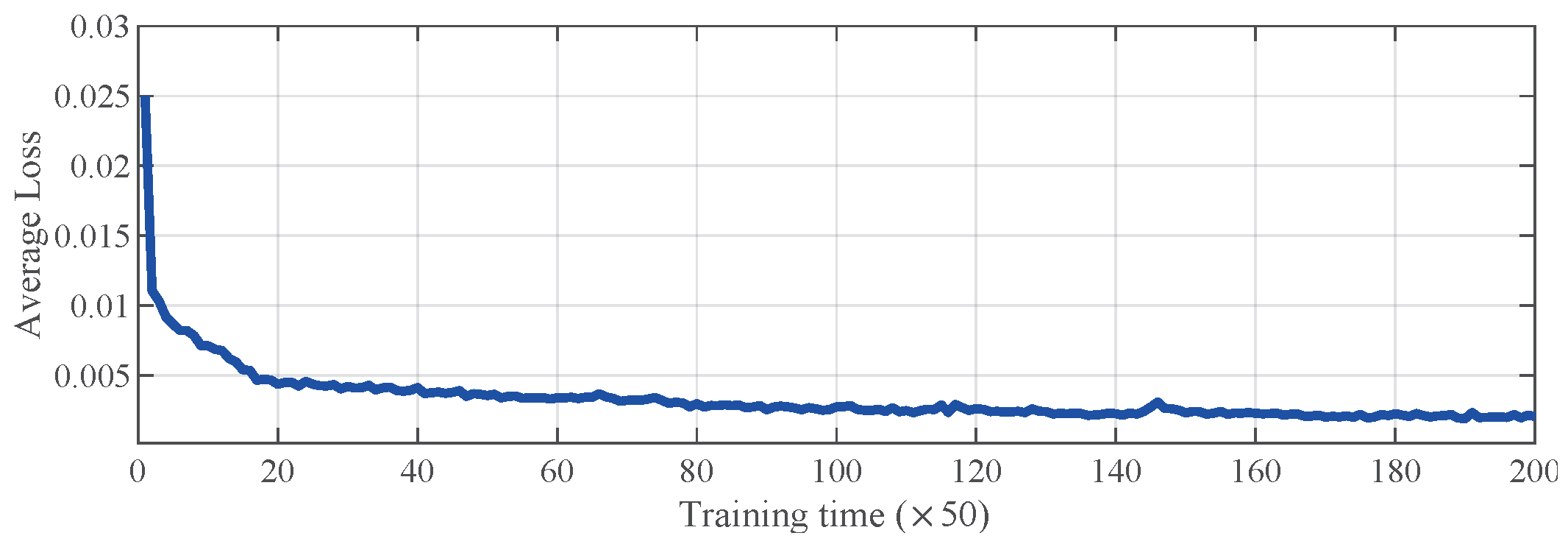
Loss function ia an key index that indicates the accuracy of the proposed method, and the testing set are employed to optimization of the parameters of proposed method (e.g., weights and bias of the CNN and LSTM blocks). The total loss of the proposed method decrease rapidly during 0–20 training periods and then stabilizes in a small range interval, as shown in Figure 4. The trends show that our proposed method can be a ideal method for capturing dynamic behaviors of the ADNs.

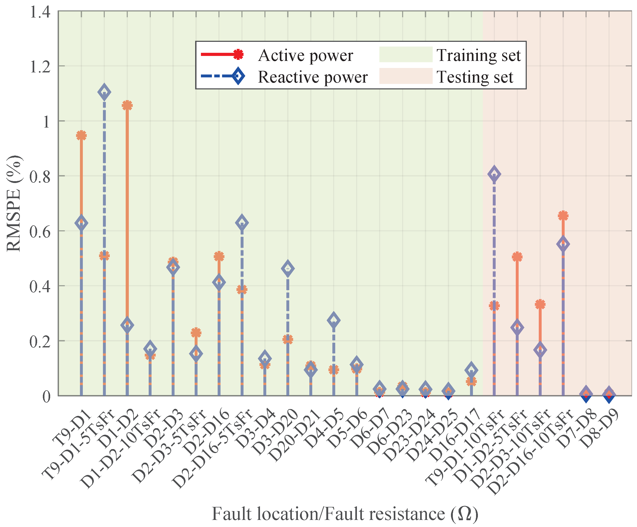
The RMSPEs between the measured values of the active and reactive power and calculated values using the proposed method under different fault locations and faults resistances are shown in Figure 5, and the green background area represents the training set, while the pink background area represents the testing set. In this figure, the x-axis represents different fault points and different fault short-circuit resistances. For example, T9-D1 denotes that the disturbance occurs at the line between node 9 of transmission network and node 1 of distribution network, where T represents transmission network, D indicates distribution network and the number is the node number. Moreover, the suffix ‘5TsFr′ and ‘10TsFr′ indicate that the short-circuit resistance is five and ten times the initial setting, respectively. And the initial setting is 1 ohm. The conclusion can be drawn as follows:

(1) When the disturbance occurs near the connection point, the error of equivalence will increase (i.e., T9-D1, D1-D2 and D2-D16), and vice versa (i.e., D6-D7, D6-D23 and D8-D9). This is because when the disturbance location is close to the connection point, the load removed due to the disturbance is relatively large, significantly impacting the entire system and thereby weakening the model′s tracking capability. The opposite is also true.

(2) In training set, the maximum and minimum RMSPE of the active power are 1.056 and 0.0108, respectively, while for reactive power they are 1.1048 and 0.0169, respectively.

(3) In testing set, the maximum and minimum RMSPE of the active power are 0.6547 and 0.0067, respectively, while for reactive power they are 0.8063 and 0.0038, respectively.

(4) The results of training set reveal that our proposed method can accurately tracking the dynamic behaviors of the ADNs and the testing results indicate our proposed method has great generalization ability for practical applications.

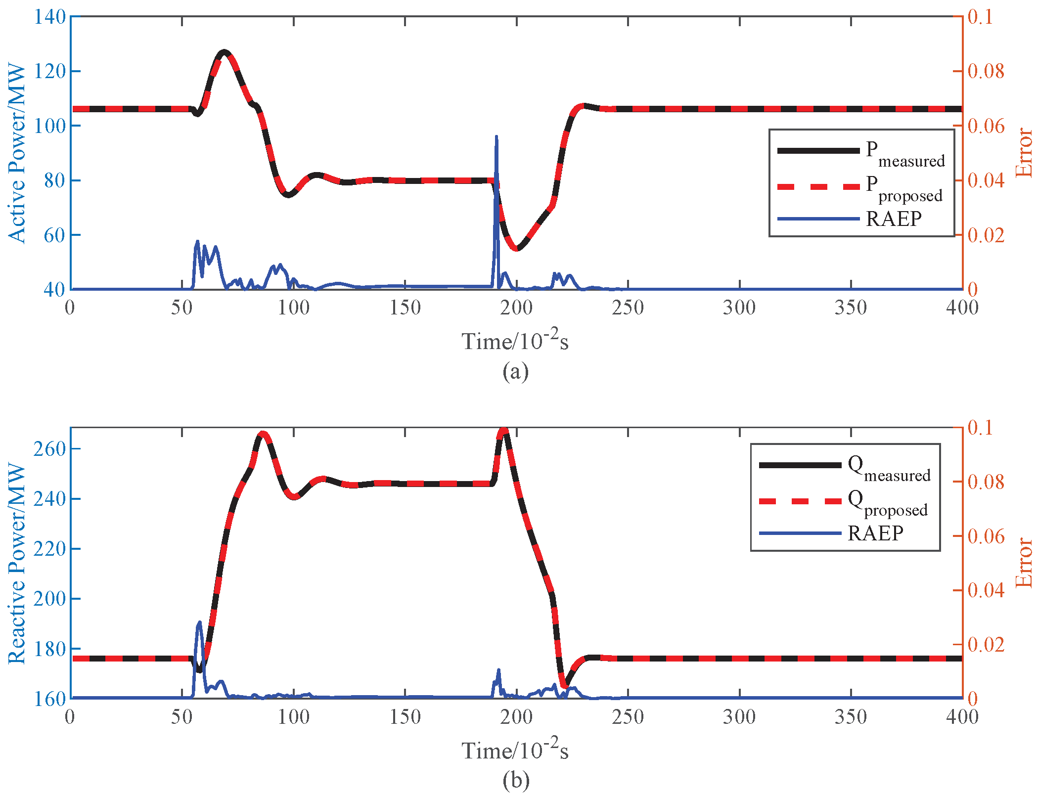
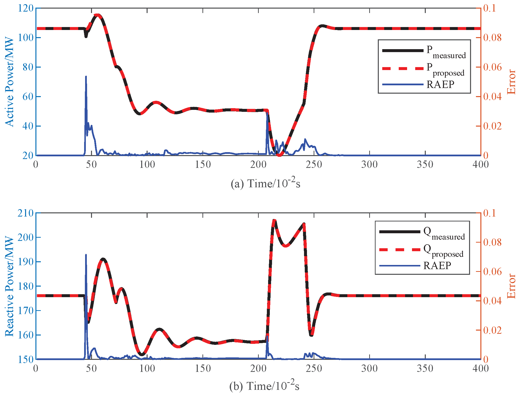
Furthermore, to better show the comparison results between the measurement results (i.e., benchmark) and the outputs of the KOA-MMFDL equivalent model, the two representative examples in training set named D1-D2-10TsFr and D2-D3 are visualized in the form of dynamic response curve, as shown in Figure 6 and Figure 7, respectively. The same visualization example called T9-D1-10TsFr and D2-D16-10TsFr in testing set are shown in Figure 8 and Figure 9, respectively.

In the visualization figures of the training set, the peak RAEP (the magenta curve) of D1-D2-10TsFr and D2-D3 for active power are 1.052% and 10.382%, respectively. For the reactive power, the peak RAPE is 1.794% for D1-D2-10TsFr and 6.1% for D2-D3. These figures present that our proposed method can fit the benchmark results well within the interval of the above proposed three states. Therefore, the results confirm that the KOA-MMFDL can accurately tracking the dynamic active and reactive response of the ADNs under different fault locations or resistances.

For the visualization illustrations in testing set, the peak error of T9-D1-10TsFr is 4.749% for real power and 11.45% for the reactive power. Similarly, the peak error of D2-D16-10TsFr is 7.707% for real power and 5.938% for the reactive power. The results in testing set indicate that our proposed method can also accurately represent the dynamic response of the ADNs, even though the disturbances of the testing set are differ from that in the training set.

Accordingly, it is clearly confirmed that our proposed method has great generalization and robustness abilities for tracking the dynamic behaviors of the ADNs under different faults conditions in power systems.

4.3. Performance Evaluation II: KOA-MMFDL Versus LSTM, RNN, ANN and MFDL

Performance evaluation II is considered to testify the equivalence accuracy of the KOA-MMFDL method by comparing with other Non mechanism method (i.e., LSTM [23], RNN [22], and ANN [19]-based equivalent method). Furthermore, in order to better demonstrate the ability of our proposed MMFDL to capture the relationship between multi-scale voltage input and power output, a model that does not consider multi-scale voltage input (i.e., multimodal fusion deep learning) called MFDL is employed as a comparison model. The MFDL is constructed with the same structure of that MMFDL.

Table 2. Active response Comparisons between KOA-MMFDL method and MFDL, LSTM-, RNN-, ANN-based equivalent method.

Num	Fault Location/ Fault Resistance (Ω)	RMSPE of Active Power
		Proposed	MFDL	LSTM	RNN	ANN
1	D1-D2	1.056	1.0511	1.1315	1.364	2.6493
2	D1-D2-5TsFr	0.5047	0.5207	0.8336	1.1634	1.2283
3	D2-D3	0.4863	0.5122	0.7911	0.8415	0.8215
4	D2-D3-5TsFr	0.2288	0.3958	0.5114	0.8681	0.8188
5	D2-D16	0.5065	0.7495	0.8572	0.9736	0.8572
6	T9-D1-5TsFr	0.5091	0.9038	1.1621	1.1768	1.2687

and

Table 3. Reactive response Comparisons between KOA-MMFDL method and MFDL, LSTM-, RNN-, ANN-based equivalent method.

Num	Fault Location/ Fault Resistance (Ω)	RMSPE of Reactive Power
		Proposed	MFDL	LSTM	RNN	ANN
1	D1-D2	0.2525	0.458	0.748	1.3743
2	D1-D2-5TsFr	0.2481	0.3195	0.9611	0.7551	1.0608
3	D2-D3	0.4673	0.861	0.8786	1.0279	0.9349
4	D2-D3-5TsFr	0.1529	0.6258	0.6274	0.7631	0.7571
5	D2-D16	0.4127	0.8642	0.8685	1.4177	0.8685
6	T9-D1-5TsFr	1.1048	1.3618	1.5696	3.1337	4.1526

shows the RMSPEs of KOA-MMFDL, MFDL, LSTM, RNN and ANN for both active power and reactive power in 6 scenarios of IEEE-14 transmission network and IEEE-33 distribution networks.

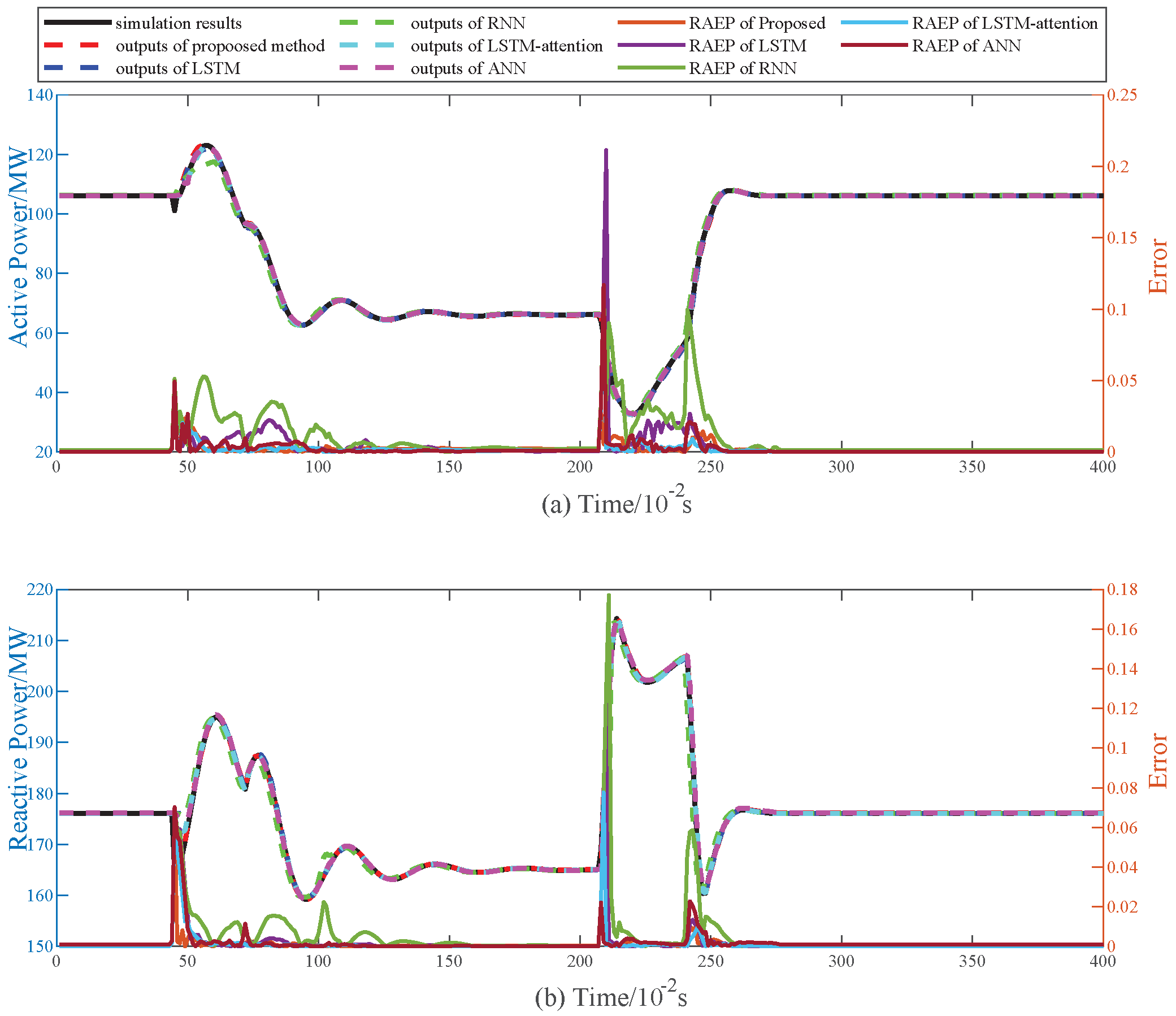
Moreover, to more intuitively demonstrate the differences in performance between our proposed method and other non-mechanism methods, we randomly selected a set of case from Table 3 for visualization. The comparison results are shown in Figure 10. The red, blue, green, cyan and magenta dashed curves are dynamic behaviors of ADNs with the KOA-MMFDL, MFDL, LSTM, RNN and ANN equivalent method, respectively. The following conclusion can be drawn:

(1) In Table 3, the ANN equivalent method performs worst among the other five methods in most cases (i.e., D1-D2 and T9-D1-5TsFr).

(2) The ANN equivalent method and RNN equivalent method mismatch the targets in the beginning of the second stage and the third stage in Figure 10, but the ANN method outperforms the RNN method.

(3) The LSTM equivalent method and MFDL match the targets better than RNN and ANN methods in most of testing sets, but MFDL method outperforms the LSTM method.

(4) The KOA-MMFDL equivalent method reaches the best fit among all five methods.

(5) The performance of our proposed method is better than MFDL, indicating that the multi-scale voltage feature input we considered can better capture the relationship between voltage and power.

(6) Finally, the performance of MFDL and KOA-MMFDL are better than other single modal methods (or non-mechanism methods), denoting that multimodal methods are superior than single modal method.

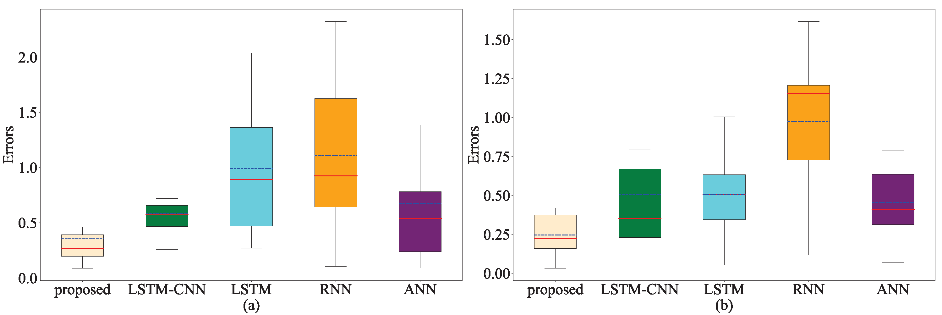
Moreover, we also plot the boxplot of PQ error of each model for all case listed in Table 3 as shown in Figure 11. The box lengths of the RNN-based equivalent model are the longest, indicates that the fitting robustness of the RNN-based is worse than that of other equivalent model. What′s more, compared with other single equivalent model, the box lengths of our proposed equivalent model and LSTM-attention model are shorter than that of other methods, indicates the better fitting effect and robustness, but the performance of LSTM-attention equivalent model is less optimistic than our proposed method.

Therefore, based on the above comparison results, it is confirmed that our proposed method is more suitable for tracking the dynamic behaviors of ADNs than other methods.

4.4. Performance Evaluation III: KOA-MMFDL Versus Manually Set MMFDL1, MMFDL2 and MMFDL3

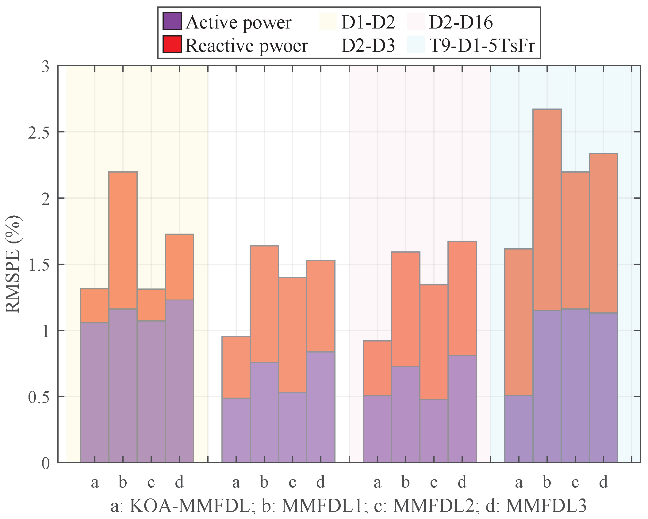
The performance of KOA-MMFDL are also compared with three MMFDLs with different structures to validate the effectiveness of the KOA. The sum of the active power error and reactive power error is shown in Figure 12. The four areas with different background colors represent different fault locations or resistances, and the meanings are same as Figure 5. Figure 12 indicates following:

(1) The KOA-MMFDL method achieved a minimum total RMSPE of 0.9192, comprising an active power error of 0.5065 and a reactive power error of 0.4127, representing the lowest values among all compared models.

(2) The KOA-MMFDL method outperforms best among other manually set MMFDL methods in all cases.

(3) The performance of MMFDL has been greatly improved through automatically tuning the adjustable parameters (especially the depth of LSTM and FC layers) by KOA.

5. Conclusions

In this article, a KOA-based multiscale and multimodal fusion deep learning equivalent method is proposed to represent the dynamic behaviors. The proposed method incorporates two modalities: one is a CNN+attention module, which simulates the voltage equation of the correction nodes in the NRPFC to perceive the dynamic behavior of the ADN; the other is an LSTM+FC module aggregated through a multi-scale fusion approach with different voltage input windows, enabling a better capture of the relationship between voltage and power from the perspective of DAE. Then, KOA was employed for automatically optimizing parameter of MMFDL, especially the depth of LSTM and FC layers, rather other manual setting. To verify the effectiveness of KOA-MMFDL, an IEEE 9-bus transmission network combined with an modified IEEE 30-bus distribution network are chosen as the testing system. The simulation indicates that the proposed KOA-MMFDL equivalent method can accurately tracking the dynamic behaviors of ADNs under various disturbance conditions. Furthermore, compared with MFDL, LSTM, RNN and ANN equivalent methods, the performance of KOA-MMFDL equivalent method outperform the other methods in the study cases. It can also validated that the multiscale fusion method for aggregating load modeling models with different voltage input size can better capture the relationships between voltage inputs and power outputs from the aspect of DAEs. In addition, with the heip of KOA, we can automatically adjust the hyperparameters of model instead of trial and error, which greatly save modeling time. The simulation also shows the effectiveness of KOA in automatic parameter adjustment.

Although the proposed KOA-MMFDL can automatically tune the parameters in MMFDL, the fitness evaluation costs much time in the whole process of MMFDL. To address this limitation, we can employ Bayesian optimization to further accelerate the tuning time in further work. In addition, the potential fault cases include the faults located in other nodes which far from boundary bus, the faults with more larger or small resistance and the faults with other topology reconstructions. These potential cases is also challenge for the dynamic equivalent of ADNs, and is also a problem that we need to solve in our future work.

Finally, the proposed KOA-based multiscale and multimodal fusion deep learning equivalent can also be employed for power stability control and voltage stability evaluation in power system analysis.