Article

Analysis of a Three-Echelon Supply Chain System with Multiple Retailers, Stochastic Demand and Transportation Times

by
Georgios Varlas
1,
Stelios Koukoumialos
2,
Alexandros Diamantidis
3 and
Evangelos Ioannidis
3,*
1
Department of Business Administration, University of the Aegean, 82100 Chios, Greece
2
Department of Business Administration, University of Thessaly, 41500 Larissa, Greece
3
Department of Economics, Aristotle University of Thessaloniki, 54124 Thessaloniki, Greece
*
Author to whom correspondence should be addressed.
Mathematics 2025, 13(19), 3199; https://doi.org/10.3390/math13193199
Submission received: 5 August 2025 / Revised: 13 September 2025 / Accepted: 23 September 2025 / Published: 6 October 2025

Abstract

In this paper we present an exact numerical model for the evaluation of a three-echelon supply chain with multiple retailers. Poisson demand, exponentially distributed transportation times and lost sales at the retailers are assumed. The system is modeled as a continuous time Markov chain, and the analysis is based on matrix analytic methods. We analyze the infinitesimal generator matrix of the process and develop an algorithm for its construction. Performance measures for the system are calculated algorithmically from the stationary probabilities vector. The algorithm is used for an extensive numerical investigation of the system so that conclusions of managerial importance may be drawn.
MSC:
60J27; 60J28; 90B06; 90B05
JEL Classification:
C44; C6; C02

1. Introduction

Multi-echelon inventory systems with multiple retailers have practical importance, but their modeling can become highly complex, sometimes even to the point of mathematical intractability. In general, to tackle complexity either simplifying assumptions must be made (deterministic parameters, no stock-outs, nested policies) or approximate methods have to be employed. Both approaches have their respective drawbacks, and there is an ongoing search for more realistic models that would allow us to assess longer and more complex supply chains.
In this paper we propose an algorithm for the exact numerical evaluation of performance measures for a three-echelon system with multiple retailers. Our modeling approach is based on the analysis of the infinitesimal generator matrix, and it allows us to use more realistic assumptions such as stochastic demand, stochastic transportation times and lost sales in case of stock-out. The resulting model is used for an extensive numerical research so that conclusions of managerial importance can be drawn.

2. Literature Review

A great part of the literature on divergent systems is concerned with two-echelon systems with one wholesaler and multiple retailers (OWMRs). An introduction to the evaluation of such systems is given in [1]. A systematic review of systems with periodic review inventory control policies can be found in [2]. An overview of some of the OWMR-related literature is given in Table 1.
Analyses of divergent systems with more than two echelons are less common. In [3] the authors analyze a multi-echelon system with general arborescent topology. They assume backordering, demand with Poisson characteristics and zero lead times. They define the system as a Markov process and characterize the optimal cost, applying dynamic programming that provides numerical approximations for global optimization.
Table 1. Related Literature.
Paper/Review PolicyDemandTransportation TimeShortages at the RetailerMethod
[4]/Mixed continuous–periodic review policyPoissonDeterministicBackordersApproximation method
[5]/Single cycleConstantInstantaneousNo shortagesClosed form
[6]/Stationary nested policiesDeterministicNegligibleNo shortagesHeuristic
[7]/Stationary nested policiesConstantInstantaneousNo shortagesSearch algorithm based on the characteristics of the optimal cost curve
[8]/PeriodicRandomConstantBackordersClosed form
[9]/Single cycleDeterministicNegligibleNo shortagesOrder interval division and recursive tightening
[10]/Integer-ratio policiesDeterministicNegligibleNo shortagesIterative procedure based on the balance between the
replenishment and the inventory holding costs
[11]/Periodic–finite planning horizonStochastic (Poisson/normal)ZeroLost salesApproximate dynamic programming/stochastic dynamic programming
[12]/PeriodicCorrelated/bivariate PoissonConstant (1 period)Lost salesRestricted observation Markov decision process
[13]/PeriodicCorrelated with inventory and priceConstantNo shortagesGenetic algorithm/fuzzy simulation
[14]/Periodic base stockDeterministicConstantLost salesMathematical programming/genetic algorithms
[15]/Continuous review (R,Q) policiesPoissonConstantBackordersApproximate optimal solutions
[16]/Finite horizon policyDeterministic dynamicNegligibleNo shortagesInteger programming
[17]/Periodic (s,nq) for warehouse/discrete base stock policy for retailersStationary i.i.d.
random
DeterministicBackordersDecomposition
[18]/Periodic, integer ratio, echelon stock, order up to policiesPoissonConstantBackordersExact solution based on the regenerative cycle
[19]/Periodic finite horizon policyDeterministic dynamicDeterministicBackorders/lost salesDecomposition
[20]/Cross-docking warehouse/(1,T) policy for retailersPoissonConstantLost salesHeuristic
[21]/Periodic review base stock, finite horizonDeterministic dynamicConstantBackordersMixed-integer linear programming
[22]/Continuous review (S−1,S) for the retailers, no replenishment policy for the warehouseStochasticStochasticBackordersSimulation
[23]/Continuous reviewDeterministicNormalBackordersNumerical iterative algorithm
[24]/VMI policyDeterministicDeterministicNo shortagesInteger non-linear programming/imperialist competitive algorithm
[25]/Periodic review base stockDeterministicConstantBackordersMixed-integer linear programming/heuristic
[26]/Shipments at regular intervalsDeterministicDeterministicNo shortagesIterative procedure based on the concavity property of total profit
[27]/Periodic, finite horizon, option for delayed distributionStochasticNegligibleLost salesRecursive solution algorithm based on multi-stage stochastic programming
[28]/Continuous reviewCompound PoissonConstantBackordersExact analysis of the system based on the probability mass function (pmf) of each retailer’s inventory level
[29]/Periodic with an integer-ratio ordering schedulePoissonConstantBackordersExact solution based on regenerative cycles
[30]/PeriodicPoisson/GaussianConstantLost sales/partial or complete backorderingDeep reinforcement learning
[31]/PeriodicSeasonal/stochasticNo lead timeBackordersDeep reinforcement learning and multi-stage stochastic programming
In [32] the authors investigate a system with multiple stocking echelons and multiple retailers. They formulate a model for a mixed produce-to-order and produce-in-advance inventory system and seek to determine the optimal inventory at each installation on a single-period basis. They analyze the system for uniform and normal external demand with allowed transshipments between the retailers, and they conclude that in both cases the problem can be solved as a constrained optimization problem.
In [33] a model for a three-tier system with one supplier, one manufacturer and multiple retailers is developed. The retailers’ demands are random variables with generic probability density functions and lost sales are allowed. The model is based on a single cycle basis and a procedure for its solution is proposed. The authors focus on the comparison of traditional policies, where every node acts independently, to consignment policies where the retailers and the supplier are subordinates of the manufacturer.
The author in [34] develops approximation algorithms for optimal solutions for k-echelon divergent systems in a deterministic setting, with or without backorders. His approach is based on the decomposition technique.
In [35,36] an integrated three-level supply chain with a distribution structure, where one production plant serves multiple warehouses and each warehouse may serve many retailers, is examined. Both works assume dynamic and known demand over a discrete and finite planning horizon. In [35] the authors assume un-capacitated shipments, and they expand on the OWMR solutions. The authors compare different mixed-integer programming formulations for the optimal lot sizing, scheduling, transportation and warehousing decisions. In [36] limited production and transportation capacity, retailers that may change supplier over the planning horizon, as well as the possibility that the demand from a specific period may be satisfied by deliveries over multiple periods is assumed. The authors propose two heuristic algorithms for the optimal solution of the problem as well as an exact brunch and cut algorithm.
In [37] the authors employ mixed-integer programming techniques. They investigate three-level systems with multiple retailers, each one of which is supplied by a predefined warehouse, while the warehouses are supplied by a single production plant. The retailers face deterministic dynamic demand over a finite planning horizon, while it is assumed there is no restriction on the amount that can be produced or transported in a given period. The authors propose approaches for more effective and efficient optimal solutions with regard to the total cost incurred.
In [38] a multi-product integrated four-level supply chain consisting of a supplier, a producer, a wholesaler and multiple retailers is considered. Demand and lead times are deterministic, the review policy is periodic, and shortages occur at the retailers. The authors assume that the order quantity of products in each one of the levels has a normal distribution, while all the levels of the supply chain orders have the same number of products during the same period length. They formulate the problem as a non-linear programming model, and they apply two different approximation algorithms (sequential quadratic programming and interior point with super-linear convergence rates) in order to optimize the number and volume of the stockpiles.
The authors in [39] investigate both divergent and general structure systems that are centrally controlled. The authors assume periodic review policies with backorders and take into consideration both lead time and demand uncertainties. They model the problem as a Markov decision process and then they apply deep reinforcement learning and the proximal policy optimization algorithm for an approximate solution that minimizes the holding and backorder costs.
A dynamic supply chain member selection algorithm based on conditional generative adversarial networks (CGANs) is presented in [40]. For the analysis and the prediction of purchase and inventory links in the supply chain, machine learning is also used. They also examine the vehicle scheduling module where the path is reasonably planned to improve the operation efficiency. Finally, they use the SSH framework for the integrated implementation of the SCM system.
Inventory policies for Lindley systems with possibly unbounded costs, using as an objective the minimization of the expected discounted total cost by ordering (production) strategies are examined in [41]. The authors also show the existence of a subsequence of minimizers of the value iteration functions that converge to an optimal inventory system policy.
A systematic review of the existing state-of-the-art literature on machine learning (ML) in logistics and supply chain management (LSCM) is given in [42]. A wide collection of eight databases from 1994 to 2019 are explored. In total, 110 articles are analyzed showing that only nine literature reviews have been published in this area. The most important key findings show that 53.8% of publications were closely clustered on transportation and manufacturing industries and 54.7% were centered on mathematical models and simulations.
In this paper we propose an algorithm for the exact numerical evaluation of a three- echelon system consisting of a distribution center, a wholesaler and multiple retailers. We assume continuous review inventory control policies with each installation following an independent (s,Q) policy. Both demand and transportation times are assumed to be stochastic, while demand that cannot be met from inventory on hand at the retailers is assumed to be lost. The system is modeled as a continuous time discrete state Markov process, and the analysis is based on the infinitesimal generator matrix. In comparison with existing models, we investigate a longer network under more realistic stochastic conditions, and we offer an exact solution. Moreover, whereas most of the existing literature focuses on the optimal solution, our investigation is concerned with the general behavior of the system. In practice, optimal policies are not always easy to find or follow, and we consider it important to understand the effect of small changes in structural and operational parameters on the overall system performance, even when operating in sub-optimal conditions. The proposed algorithm could be used as the evaluative tool in the context of an optimization algorithm.

3. System Description

We investigate a pull system of three tiers with multiple retailers. A distribution center (DC) orders from a plant and supplies a wholesaler. In its turn, the wholesaler supplies n independent retailers (Figure 1). Each member holds an inventory and follows an independent continuous review inventory control policy (s,Q). The external demand has pure Poisson characteristics (exponentially distributed inter-arrival times and unitary demand per customer), while the external demand that cannot be met from the inventory on hand at each retailer is lost. In case of a stock-out at the wholesaler, the highest indexed retailer always has priority (retailer i has priority over retailer i − 1). Transportation times are exponentially distributed and independent of the replenishment order quantity, while both the DC and the wholesaler may send partial orders. The transportation processes are modeled as virtual independent stations. On replenishment order initiation, the respective inventory is subtracted from the upstream node and remains “in transit” until its delivery to the downstream node. The plant is assumed to be saturated, always sending complete orders of Qd units to the DC. It is also assumed that at any given time at most one order can be in transit to any given node (one outstanding order assumption). Such an assumption is common in analytic models, and it is necessary in order to maintain a tractable level of complexity [43].
  • For our analysis we denote as the decision variables the number of retailers and the parameters of the inventory control policies at each node:
  • n: the number of retailers
  • sd: the reorder point at the distribution center
  • Qd: the replenishment order quantity at the distribution center
  • sw: the reorder point at the wholesaler
  • Qw: the replenishment order quantity at the wholesaler
  • si: the reorder point at retailer i
  • Qi: the replenishment order quantity at retailer i
  • The other parameters that are necessary to completely define the system are as follows:
  • μd: the transportation rate for orders from the plant to the distribution center
  • μw: the transportation rate for orders from the distribution center to the wholesaler
  • μi: the transportation rate for orders from the wholesaler to retailer i
  • λi: the arrival rate of external customers at retailer i

4. Modeling Approach

Our modeling approach is based on the analysis of the infinitesimal generator matrix of the process. The system is modeled as a continuous time, discreet state Markov chain with a finite and multi-dimensional state space. We start by defining the state space of the process and by prescribing rules for ordering the permissible states. The resulting infinitesimal generator matrix G is partitioned into recurring blocks of states (sub-matrices), with different kinds of blocks corresponding to different kinds of transitions. In general, matrix G has a three-tier structure. Blocks on the diagonal describe transitions in the retailers for a given state of the upstream part of the system, with each basic level corresponding to a different level of inventory on hand at the distribution center. Blocks above the diagonal describe the arrival of a replenishment order at the distribution center (“birth” transitions), while blocks below the diagonal correspond to changes at the wholesaler. Transitions between non-adjacent basic levels are generally allowed.
Given the generator matrix, it is easy to construct a linear system of balance equations and compute a vector of stationary probabilities. For the results presented here, we have used LU factorization with partial pivoting from the Matlab© toolbox. System performance measures can be computed algorithmically from the stationary probabilities, taking advantage of the predefined ordering of states.
This section may be divided by subheadings. It should provide a concise and precise description of the experimental results, their interpretation, as well as the experimental conclusions that can be drawn.

4.1. States Definition

The system is modeled as a (2n + 3) dimensional continuous time Markov chain. At any given time t ≥ 0, the state of the system can be defined by a 2n + 3 dimensional vector I d t , T w , t I w t , T n t , I n t , T n 1 t , I n 1 t , , T 1 t , I 1 t , where
  • I d t : the inventory on hand at the distribution center at time t with 0 ≤ I d t ≤ sd + Qd
  • T w t : the inventory in transit to the wholesaler at time t with 0 ≤ T w t Qw
  • I w t : the inventory on hand at the wholesaler at time t with 0 ≤ I w t ≤ sw + Qw
  • T i t : the inventory in transit to retailer i at time t with 0 ≤ T i t ≤ Qi
  • I i t : the inventory on hand at retailer i at time t with 0 ≤ I i t ≤ si + Qi
The Markov process has a finite state space and its dimension, which depends on the decision variables, can be calculated algorithmically. In general, for computational reasons, transient states are not taken into consideration, except where it simplifies the algorithmic analysis. The states are ordered using a lexicographical order. The subset of all states corresponding to the fixed inventory at the distribution center (Id) is taken as the basic level, and the basic levels are ordered from lower to higher. Within each basic level, the states are ordered according to the inventory in transit to the wholesaler (Tw), then according to the inventory at the wholesaler (Iw) and finally according to Ti and Ii, with higher priority retailers preceding lower priority ones and lower values preceding higher values.
The four kinds of events that may instantaneously alter the state of the system are as follows:
  • The arrival of an outstanding order from the Plant to the Distribution Centre I d t + d t = I d t + Q d
  • The arrival of an outstanding order from the DC to the wholesaler I w t + d t = I w t + T w t
  • The arrival of an outstanding order at retailer i  I i t + d t = I i t + T i t
  • The occurrence of external demand at retailer i  I i t + d t = I i t 1
For example, for the simple system with two retailers and parameters sd = 0, Qd = 2, sw = 0, Qw = 2, s1 = 2, Q1 = 2, s2 = 0, Q2 = 1, the system is modeled as a seven-dimensional continuous time Markov chain { I d t , T w t , I w t , T 2 t , I 2 t , T 1 t , I 1 t , t 0 } with 163 possible states. Assuming that we start at state (0,0,2,0,1,1,1), the possible transitions and associated events are
-
To state (0,0,0,0,1,2,2) with transition rate μ1—Arrival of a replenishment order at retailer 1 and triggering of a new replenishment order from the wholesaler to retailer 1;
-
To state (0,0,1,1,0,1,1) with transition rate λ2—Occurrence of external demand at retailer 2 and triggering of a replenishment order from the wholesaler to retailer 2.
-
To state (0,0,2,0,1,1,0) with transition rate λ1—occurrence of external demand at retailer 1.
-
To state (2,0,2,0,1,1,1) with transition rate μd—Arrival of a replenishment order at the DC.

4.2. The Infinitesimal Generator Matrix

Diagonal blocks describe transitions where only the state of the retailers may change (inventory at the DC, inventory at the wholesaler and inventory in transit to the wholesaler do not change). The structure of these blocks can be defined recursively. We use as the “seed” the block describing transitions for the lowest priority retailer (retailer 1) and its associated transport station. The block for each successive retailer is constructed using as the “building block” the block for the previous retailer and according to rules that hold for all retailers. The specific structure for each such block depends on whether it corresponds to I w t = 0 , or I w t > 0 .
As an example we analyze the structure of the diagonal blocks when I w t > 0 . We define the following:
  • b s d : the greatest common divisor of ( Q d , Q w )
  • b s w : The greatest common divisor of b s d , Q 1 , Q 2 , , Q n
  • q i : the integer part of Q i b s w
Block C1 for transitions where only the state of retailer 1 is changed ( I 1 t or T 1 t ) is a square matrix of C l 1 = Q 1 + q 1 ( s 1 + 1 ) dimension (Figure 2). C1 can be further reduced into smaller blocks. For example, block C 1 z is a Q 1 × Q 1 matrix for T 1 t = 0 , I 1 t > s 1 :
Block C2 includes transitions where only the state of retailer 1 or 2 is changed (Figure 3). For every state of retailer 2, there are C l 1 possible states of retailer 1. C2 is a square matrix with a dimension of C l 2 = Q 2 C l 1 + q 2 ( s 2 + 1 ) C l 1 . Correspondingly, C 2 z for T 2 t = 0 , I 2 t > s 2 is a Q 2 C l 1 × Q 2 C l 1 matrix. If I1 is the identity matrix of Cl1 dimension
In general, block Ci (i > 2) includes transitions where only the state of retailers 1 to i may be changed (Figure 4). For every state of retailer i, there are C l i 1 possible states of the retailers with lower priority. Ci is a square matrix with dimension:
C l i = Q i C l i 1 + q i ( s i + 1 ) C l i 1 ,   where   C l i 1 = Q i 1 C l i 2 + q i 1 ( s i 1 + 1 ) C l i 2
Accordingly, C i z for T i t = 0 , I i t > s i is a Q i C l i 1 × Q i C l i 1 matrix, where Ii−1 is the identity matrix of the Cli−1 dimension:
Above the diagonal there are diagonal blocks of μd describing the arrival of a replenishment order at the distribution center (DC). An outstanding replenishment order from the plant to the DC occurs as long as I d t s d , and according to our assumptions, Qd units are always delivered. When there is no outstanding demand from the wholesaler, the incoming order increases the available inventory on hand at the DC I d t + d t = I d t + Q d . In the case of DC stock-out ( I d t = 0 , T w t = 0 , I w t s w ), part or all of the incoming replenishment order is immediately forwarded to the wholesaler, and the μd blocks are moved appropriately to the left.
The blocks below the diagonal correspond either to the arrival of a replenishment order at the wholesaler or the triggering of a replenishment order to the retailers. In the first case, there are blocks of μw which occur as long as I w t s w . A full or a partial order may be delivered, and the exact position of each μw element in the infinitesimal generator matrix depends on the values of I d t and I w t . When I w t = 0 and there are pending orders from the retailers, part or all of the incoming replenishment order is forwarded to the retailers, according to the priority of each retailer. When I d t > 0 , a new replenishment order will be triggered if I w t + d t s w .
The triggering of a replenishment order to a retailer can occur when (A) external demand occurs at retailer i, while I i t = s i + 1 and (B) a replenishment order arrives at the retailer i, and the updated I i t + d t is less than or equal to si. In some cases a replenishment order from the DC to the wholesaler can also be triggered by these events. The corresponding blocks consist of λi and μi and are constructed recursively starting from the block for the retailer with the lowest priority (1), in a way similar to that presented for the diagonal blocks. The exact structure and positioning of the blocks depend on whether there is more than enough inventory to meet the retailer’s demand   I w t + d t > 0 , or there is just enough or not enough inventory to meet the retailer’s demand   I w t + d t = 0 . The position of the blocks also depends on whether there is inventory on hand at the DC ( I d t > 0 or I d t = 0 ) and on whether there is already a replenishment order in transit to the wholesaler ( T w t > 0 or T w t = 0 ).
The solution algorithm can be summarized in the following steps:
  • Step 1: Calculate infinitesimal generator matrix parameters from system parameters (number of basic levels, number of possible inventory levels at each stage, maximum inventory levels where outstanding orders occur)
  • Step 2: Create diagonal blocks
    • Step 2.1: Create diagonal block B1 for lowest priority retailer 1 and I w t = 0
    • Step 2.2: Through an iterative process, create diagonal block Bn for highest priority retailer n and I w t = 0 based on block Bn−1
    • Step 2.3: Create diagonal block C1 for lowest priority retailer 1 and I w t > 0
    • Step 2.4: Through an iterative process, create diagonal block Cn for highest priority retailer n and I w t > 0 based on block Cn−1
    • Step 2.5: Create the diagonal tier of the infinitesimal generator matrix using blocks Bn and Cn
  • Step 3: Insert upper diagonal blocks
    • Step 3.1: Insert blocks for the cases when I d t > 0
    • Step 3.2: Insert blocks for the cases when I d t = 0 (DC stockout)
  • Step 4: Insert below the diagonal blocks
    • Step 4.1: Add blocks corresponding to the arrival of a replenishment order at the wholesaler
    • Step 4.2: Add blocks corresponding to triggering of a replenishment order to a retailer
  • Step 5: Calculate numerically the vector of stationary probabilities (steady state solution)
    using the following algorithm (see Calculation of the steady-state probabilities below)
  • Step 6: Calculate performance measures algorithmically from the vector of stationary probabilities
The calculation of the stationary probabilities (Step 5) of the previous algorithm can be achieved using the following algorithm:
  • Calculation of the steady-state probabilities
Let n be the number of states of the system, A be the infinitesimal generator matrix with dimension (n × n), X be the matrix of the unknown steady-state probabilities with dimension (n × 1), and B be the zero matrix with dimension (n × 1)
  • Step 1: Calculate matrix A − I (I is the identity matrix)
  • Step 2: Calculate ( A I ) T (Transposition of A − I)
  • Step 3: Take ( A I ) T and replace the last row with a new row where all the elements of this new row are equal to 1. Call this new matrix P
  • Step 4: Solve the system P · X =   [ 0   0   0 1 ] T
The solution of this system provides the steady-state probabilities.

4.3. Performance Measures

Our analysis is based on the steady-state solution of the system and the numerical calculation of the vector of stationary probabilities p , where the i-th element of the vector p ( i ) corresponds to the i-th state in the hierarchy of states defined according to the lexicographical ordering. Performance measures about the system are computed algorithmically using the stationary probabilities. Some examples are given below.
  • Average inventory at the Distribution Centre—WIPd
W I P d = L e v e l = 1 N L d L e v e l b s d j = 1 L 1 p L 0 + ( L e v e l 1 ) L 1 + j
where
NLd: the integer part of s d + Q d b s d . NLd is the number of the different positive values of the inventory at the distribution centre (basic levels);
L0: the dimension of basic levels for Id = 0 (the number of all states where Id = 0);
L1: the dimension of basic levels for Id > 0 (the number of all states for any different value of Id > 0).
  • Utilization of resource for transportation towards the wholesaler—uw
Utilization of the resource for transportation to the wholesaler is the percentage of time that there is a replenishment order in transit to the wholesaler. To calculate uw we sum the stationary probabilities of states corresponding to T w t > 0
u w = i = i 0 L 0 p ( i ) + i = 1 N L d j = j 0 L 1 p ( L 0 + ( i 1 ) L 1 + j )
i 0 = B l n + N L w C l n + 1
j 0 = ( N L w n s w ) C l n + 1
NLw: the integer part of s w + Q w b s w . NLw is the number of levels of inventory on hand at the Wholesaler for I w t > 0
nsw: the integer part of s w b s w . nsw is the greatest I w t level where the wholesaler asks for a replenishment order from the DC
Bln: the dimension of the block of states comprising all possible states for the retailers for a given state of the rest of the system and I w t = 0 . The block describes transitions where only the state of the retailers is changed and its dimension can be computed algorithmically:
B l i = ( s i + Q i + 1 ) B l i 1 + n Q i ( s i + 1 ) B l i 1 ,   i     1
B l 1 = ( s 1 + Q 1 + 1 ) + n Q 1 ( s 1 + 1 )
nQi: the integer part of Q i b s w . nQi is the number of the permissible values for inventory in transit to retailer i when T i t > 0 .
  • Average inventory at the wholesaler—WIPw
WIPw is the average inventory on hand at the wholesaler. We define a vector W such that the i-th element W(i) is the probability of I w t = i . The value of each probability is computed algorithmically by summing up the appropriate steady-state probabilities. To facilitate the analysis, we break the process into four distinct cases depending on I d t and T w t values. Defining b = Bln + nsw × Cln and assuming L e v e l , L e v e l T , and L e v e l D positive integers,
I d t = 0 , T w t = 0
W ( L e v e l ) = i = 1 C l n p ( B l n + ( L e v e l 1 ) C l n + i )
1 L e v e l N L w
I d t = 0 ,   T w t > 0
W ( L e v e l ) = W ( L e v e l ) + i = 1 C l n p ( B l n + N L w C l n + ( L e v e l T 1 ) b + B l n + ( L e v e l 1 ) C l n + i )
1 L e v e l T n Q w
1 L e v e l n s w
nQw: the integer part of Q w b s d . nQw is the number of levels for inventory in transit towards the wholesaler when T w t > 0 .
I d t > 0 ,   T w t = 0
W ( L e v e l + n s w ) = W ( L e v e l + n s w ) + i = 1 C l n p L 0 + ( L e v e l D 1 ) L 1 + ( L e v e l 1 ) C l n + i
1 L e v e l D N L d
1 L e v e l N L w n s w
I d t > 0 ,   T w t > 0
W ( L e v e l ) = W ( L e v e l )         + i = 1 C l n p ( L 0 + ( L e v e l D 1 ) L 1 + ( N L w n s w ) C l n + ( L e v e l T 1 ) b + B l n + ( L e v e l 1 )           C l n + i )
1 L e v e l D N L d
1 L e v e l T n Q w
1 L e v e l n s w
Having constructed vector W, WIPw can be easily calculated as the sum:
W I P w = i = 1 N L w i b s w W ( i )
In order to calculate the retailers performance measures we define the following:
B-type blocks (Bi) such that each Bi block comprises the possible states for retailers 1 to i for a given state of the rest of the system and I w t = 0 .
C-type blocks (Ci) such that each Ci block comprises the possible states for retailers 1 to i for a given state of the rest of the system and I w t > 0 .
To facilitate the analysis, the performance measures concerning the retailers are computed by evaluating each Bn and Cn block separately. We denote L0: the dimension of basic levels for Id = 0; L1: the dimension of basic levels for Id > 0; and b = Bln + nsw × Cln. If lp + 1 the number of the first state of the Bn or Cn block under consideration and, L e v e l T , L e v e l D , and L e v e l W positive integers:
  • Bn blocks
For I d t = 0 , T w t = 0 :
l p = 0
For I d t = 0 , T w t > 0 :
l p = B l n + N L w C l n + ( L e v e l T 1 ) b
1 L e v e l T n Q w
For I d t > 0 , T w t > 0 :
l p = L 0 + ( L e v e l D 1 ) L 1 + ( N L w n s w ) C l n + ( L e v e l T 1 ) b
1 L e v e l D N L d
1 L e v e l T n Q w
  • Cn blocks
For I d t = 0 , T w t = 0 :
l p = B l n + ( L e v e l W 1 ) C l n
1 L e v e l W N L w
For I d t = 0 , T w t > 0 :
l p = B l n + N L w C l n + ( L e v e l T 1 ) b + B l n + ( L e v e l W 1 ) C l n
1 L e v e l T n Q w
1 L e v e l W n s w
For I d t > 0 , T w t = 0 :
l p = L 0 + ( L e v e l D 1 ) L 1 + ( L e v e l 1 ) C l n
1 L e v e l D N L d
1 L e v e l W N L w n s w
For I d t > 0 , T w t > 0 :
l p = L 0 + ( L e v e l D 1 ) L 1 + ( N L w n s w ) C l n + ( L e v e l T 1 ) b + B l n + ( L e v e l w 1 ) C l n
1 L e v e l T n Q w
1 L e v e l W n s w
  • Average inventory at the retailers—WIPr
WIPr is the average inventory on hand at retailer r, 1 ≤ r ≤ n.
  • B-type blocks ( I w t = 0 )
  • Retailer 1
In B1 blocks, for the states where T 1 t = 0 , positive inventory at retailer 1 corresponds to s1 + Q1 states. For T 1 t > 0 , there are nQ1 different levels of T1, while in each level s1 state, it corresponds to I 1 t > 0 . If b 1 = B l n / B l 1 the number of B1 blocks in Bn and lp + 1, the number of the first state of the Bn block under consideration is as follows:
W I P 1 B , l p = i = 1 b 1 ( j = 1 s 1 + Q 1 j p l p + ( i 1 ) B l 1 + j + 1         + j = 1 n Q 1 z = 1 s 1 z         p ( l p + ( i 1 ) B l 1 + s 1 + Q 1 + 1 + ( j 1 ) ( s 1 + 1 ) + z         + 1 ) )
  • Retailer r, 2 ≤ r ≤ n
With the same iterative approach, we can calculate the average inventory on hand for higher priority retailers. In Br blocks, for each state of retailer r correspond Blr−1 states of the lower priority retailers. In B-type blocks, for the states where T r t = 0 , inventory at retailer r can take sr + Qr values. For T r t > 0 , there are nQr different levels of T r t , while in each level sr values correspond to I r t > 0 . If b r = B l n / B l r and lp + 1, the number of the first state of the Bn block under consideration is as follows:
W I P r B 1 = i = 1 b r j = 1 s r + Q r z = 1 B l r 1 j p l p + ( i 1 ) B l r + B l r 1 + ( j 1 ) B l r 1 + z
W I P r B 2 = i = 1 b r j = 1 n Q r z = 1 s r y = 1 B l r 1 z         p ( l p + ( i 1 ) B l r + ( s r + Q r + 1 ) B l r 1 + ( j 1 ) ( s r         + 1 ) B l r 1 + B l r 1 + ( z 1 ) B l r 1 + y )
W I P r B , l p = W I P r B 1 + W I P r B 2
  • C-type blocks ( I w t > 0 )
  • Retailer 1
When T 1 t = 0 , there are Q1 different states where I 1 t > 0 . For T 1 t > 0 , there are nQ1 different levels of T 1 t , and in each level s1 state, it corresponds to I 1 t > 0 . If c 1 = C l n / C l 1 the number of C1 blocks in Cn and lp + 1, the number of the first state of the Cn block under consideration is as follows:
W I P 1 C 1 = j = 1 c 1 z = 1 Q 1 ( z + s 1 ) p ( l p + ( j 1 ) C l 1 + z
W I P 1 C 2 = j = 1 c 1 z = 1 n Q 1 y = 1 s 1 y p l p + ( j 1 ) C l 1 + Q 1 + ( z 1 ) ( s 1 + 1 ) + y + 1
W I P 1 C , l p = W I P 1 C 1 + W I P 1 C 2
  • Retailer r, 2 ≤ r ≤ n
In Cr blocks each retailer r state corresponds to Clr−1 states of the lower priority retailers. When T r t = 0 , there are Qr different values for I r t > 0 . For T r t > 0 , there are nQr different levels of T r t , while in each level correspond sr different levels of positive I r t . If c r = C l n C l r , the number of Cr blocks in Cn is as follows:
W I P r C 1 = j = 1 c r z = 1 Q r y = 1 C l r 1 ( s r + z ) p l p + ( j 1 ) C l r + ( z 1 ) C l r 1 + y
W I P r C 2 = j = 1 c r z = 1 n Q r y = 1 s r x = 1 C l r 1 y         p ( l p + ( j 1 ) C l r + Q r C l r 1 + ( z 1 ) ( s r + 1 ) C l r 1         + ( y 1 ) C l r 1 + C l r 1 + x )
W I P r C , l p = W I P r C 1 + W I P r C 2
The average inventory at retailer r (1 ≤ r ≤ n) will be the sum W I P r B , l p for Bn blocks and W I P r C , l p for Cn blocks for all possible lp.
W I P r = l p , I w t = 0 W I P r B , l p + l p , I w t > 0 W I P r C , l p
  • Stock-out probability for Retailer r—SOr
SOr is the probability that the external demand at retailer r will become lost sales. Since external demand at the retailers is independent and uniformly distributed in time, SOr will be same as the probability of inventory on hand at retailer r being zero.
  • B-type Blocks ( I w t = 0 )
  • Retailer 1
I 1 t is zero in the first state of each B1 block of states, where also T 1 t = 0 . For T 1 t > 0 , I 1 t is zero in the first state of each (s1 + 1)-dimension sub-block corresponding to a different T 1 t value. If b 1 = B l n / B l 1 ,
S O 1 B , l p = i = 1 b 1 ( p ( l p + ( i 1 ) B l 1 + 1 )       + j = 1 n Q 1 p ( l p + ( i 1 ) B l 1 + s 1 + Q 1 + 1 + ( j 1 ) ( s 1 + 1 )       + 1 ) )
  • Retailer r, 2 ≤ r ≤ n
In Br blocks, each retailer r state (r > 1) corresponds to Blr−1 states of the lower priority retailers. I r t is zero in the first Blr−1 states of each Br block of states, where T r t is also zero. For T r t > 0 , I r t = 0 in the first Blr−1 states of each (sr + 1)∙Blr−1 dimension sub-block corresponding to a particular T r t value. If b r = B l n / B l r ,
S O r B , l p = i = 1 b r ( j = 1 B l r 1 p l p + ( i 1 ) B l r + j       + j = 1 n Q r z = 1 B l r 1 p ( l p + ( i 1 ) B l r + ( s r + Q r + 1 ) B l r 1 + ( j       1 ) ( s r + 1 ) B l r 1 + z ) )
  • C-type blocks ( I w t > 0 )
  • Retailer 1
In C1 blocks I 1 t = 0 in the first state of each of (s1 + 1)-dimension sub-block corresponding to a different T 1 t value and only when T 1 t > 0 . If c 1 = C l n / C l 1 ,
S O 1 C , l p = j = 1 c 1 z = 1 n Q 1 p l p + ( j 1 ) C l 1 + Q 1 + ( z 1 ) ( s 1 + 1 ) + 1
Retailer r, 2 ≤ r ≤ n
In Cr blocks each retailer r state corresponds to Clr−1 states of the lower priority retailers. I r t = 0 in the first state of each (sr + 1)∙Blr−1 dimension sub-block corresponding to a particular T r t value and only when T r t > 0 . If c r = C l n / C l r ,
S O r C , l p = j = 1 c r z = 1 n Q r y = 1 C l r 1 p ( l p + ( j 1 ) C l r + Q r C l r 1 + ( z 1 ) ( s r + 1 ) C l r 1 + y )
Stock-out probability for retailer r (1 ≤ r ≤ n) will be the sum S O r B , l p for Bn blocks and S O r C , l p for Cn blocks for all possible lp.
S O r = l p , I w t = 0 S O r B , l p + l p , I w t > 0 S O r C , l p
  • Fill Rate of retailer r—FRr
Fill rate is the percentage of external customers arriving at retailer r whose demand is met by inventory on hand at the retailer:
F R r = 1 S O r
  • Throughput of retailer r—Thrr
Throughput is the number of product units per time unit that flow through retailer r. Alternatively, Thrr could be defined as the rate of sales at retailer r:
T h r r = λ r F R r

4.4. Validation and Model Performance

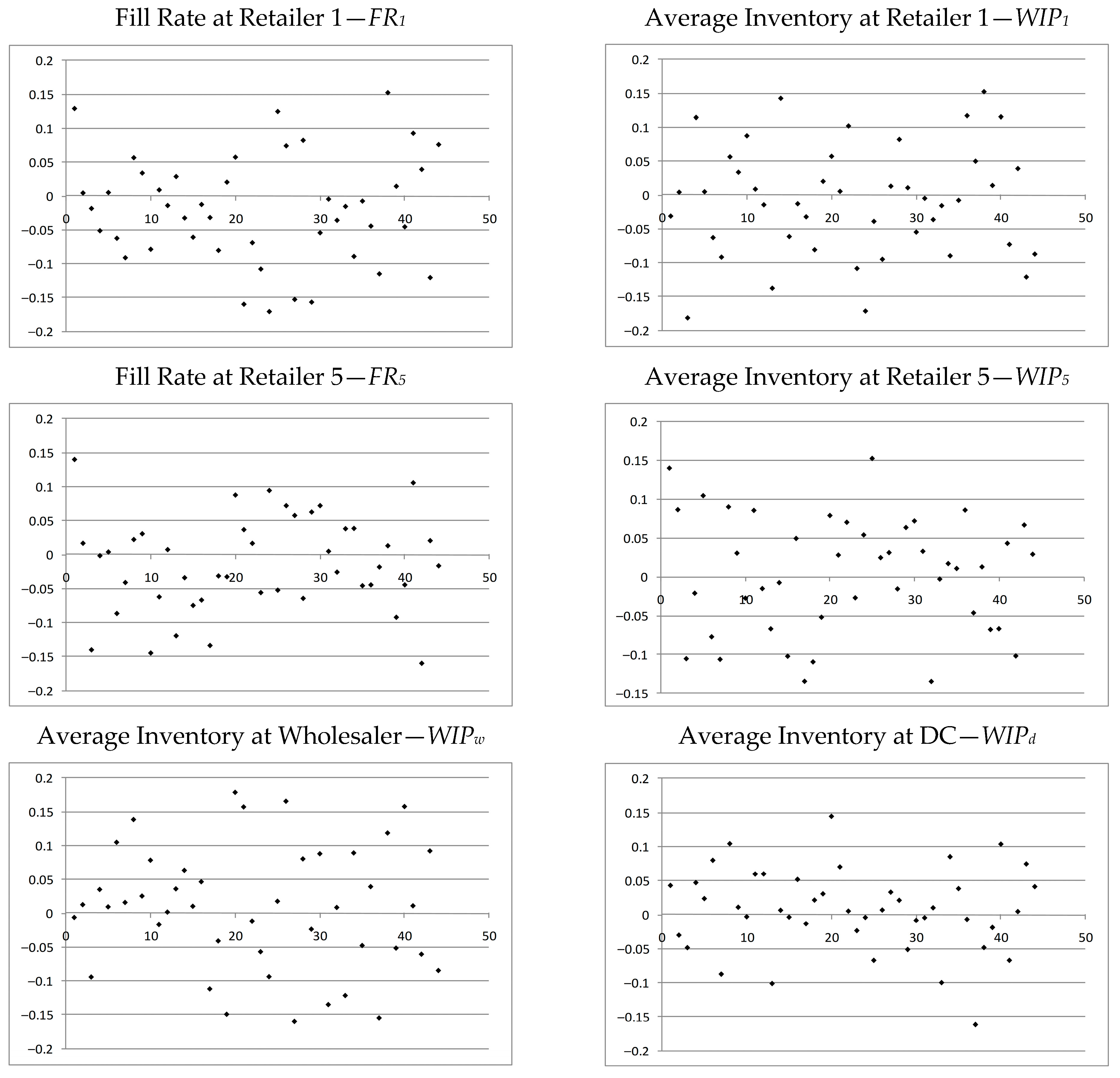
The validity of the developed algorithm was tested with simulation. A total of 900 different scenarios were tested for supply chains with one to five retailers and for various parameter relations. In all cases and for all the tested performance measures, the difference between analytic results and simulation results was within the expected deviation attributed to the experimental nature of the simulation approach. Some examples are given in Figure 5.
With regard to performance, our model shares the common problem of Markovian models, namely the increasing number of states as the system under consideration becomes bigger or more complex. As a general trend, the dimension of the infinitesimal generator matrix increases with an increasing number of retailers and increasing values for the inventory policy parameters. Regarding the computational complexity limitations, theoretically the model has no structural (mathematical) limitations. However, in practical terms, the computational feasibility is constrained by hardware resources like RAM, CPU, etc. Larger systems remain solvable but at the cost of significantly increased runtime and resource demands.
Despite size limitations, the proposed algorithm still offers certain advantages. The exact algorithm is significantly faster than simulation, in some cases the difference in computation time being several orders of magnitude. Moreover, the exact solution poses no limits on precision in contrast to simulation or approximation methods. Practitioners should consider using our model over alternatives when
  • The impact of decision variables (quantity order, reorder point, etc.) on throughput and WIP must be explicitly modeled.
  • The system properties, behavior and its sensitivity can be identified because the model is analysed explicitly. This does not hold when approximation methods are used.
  • Validation against simulation is required for credibility and decision support.
  • System design requires precise performance estimates, validated via both analytical and simulation methods.
  • Decision-makers seek to evaluate various maintenance policies under uncertainty.
A hybrid approach can also be effective: use the exact Markovian solution for small-scale cases to calibrate, validate or benchmark approximate/simulation models for larger networks.
Finally, the proposed algorithm can be easily integrated with other components in the framework of a more generic model as, for example, in the context of an optimization algorithm.

5. Numerical Results

Two different scenarios have been examined in order to check the behavior of the system and the proposed algorithm under different conditions.
The first scenario examines the case where the system is balanced (i.e., the total supply rate is equal to the total demand rate). The second scenario examines the case where the system is supply constrained. In this case the total supply rate is less than the total demand rate (i.e., demand exceeds supply). For all cases examined first the transition matrix is generated, second the steady-state probabilities are calculated, and finally the performance measures are computed according to the procedures described in the previous sections.

5.1. The Effect of Policy Parameters—Balanced Systems

We investigate “balanced” systems where upstream and downstream transportation rates are balanced. The following numerical results refer to a system with two retailers (n = 2), where μ 1 = μ 2 = λ 1 = λ 2 = μ w 2 = μ d 2 .

5.1.1. Distribution Center’s Policy (sd, Qd) for Balanced Systems

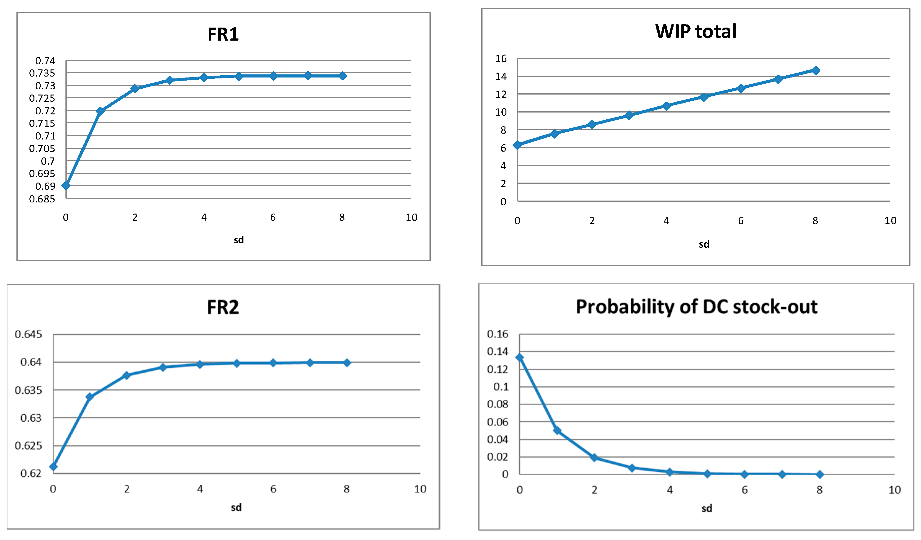
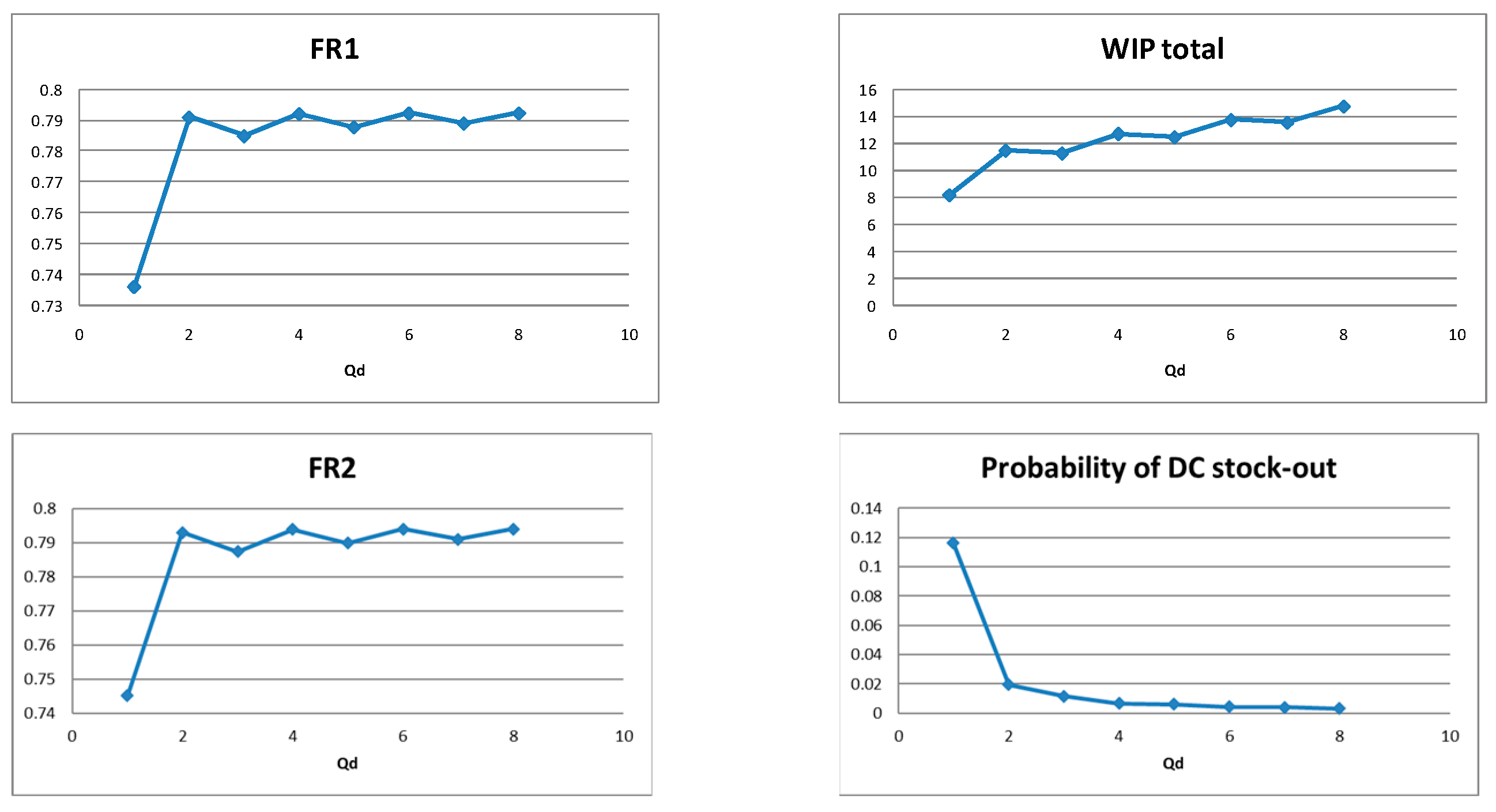
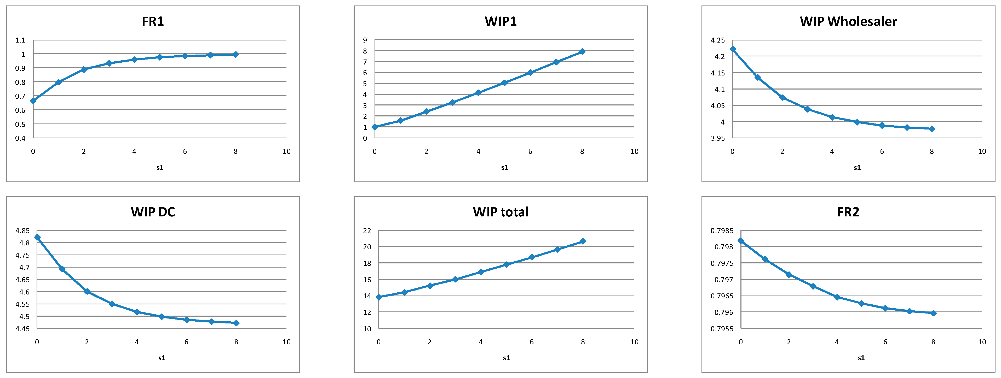
The performance of the retailers increases with increasing sd but at the cost of an increase in the average total inventory in the system (average total inventory—WIPtotal is the average inventory from the DC and downstream). Sometimes this increase is almost linear (Figure 6). The effect of Qd depends on the value of the other variables, but in general both the fill rate at the retailers and total inventory tend to increase with increasing Qd. In some cases jagged patterns are observed (Figure 7). The effects of the parameters on both retailers are similar.
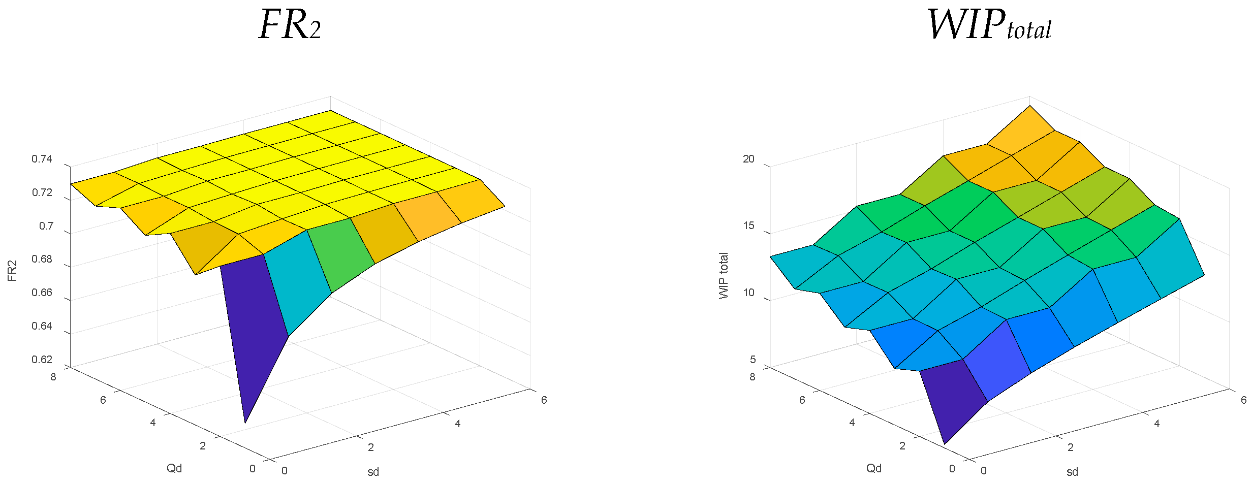
DC policy is important for the retailers’ performance only for low sd and Qd values when the distribution center is the “bottleneck” of the system (Figure 8). The presence of some safety stock at the DC seems preferable, as for sd = 0 the system is less stable and more difficult to predict. In some cases, with minor policy adjustments it is possible to achieve lower total inventory without any serious negative effect on the retailers’ performance.

5.1.2. Wholesaler Policy (sw, Qw) for Balanced Systems

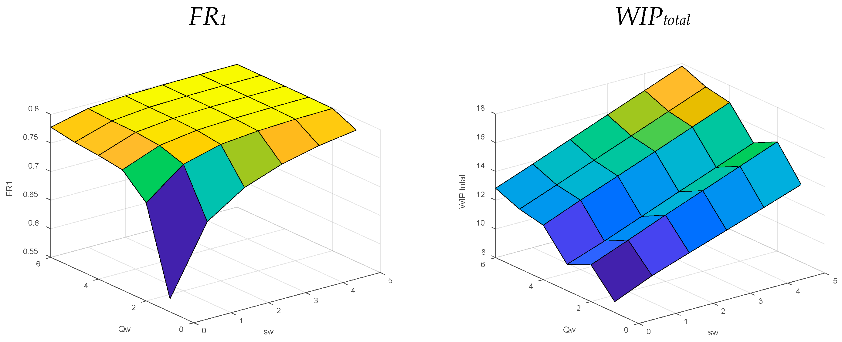
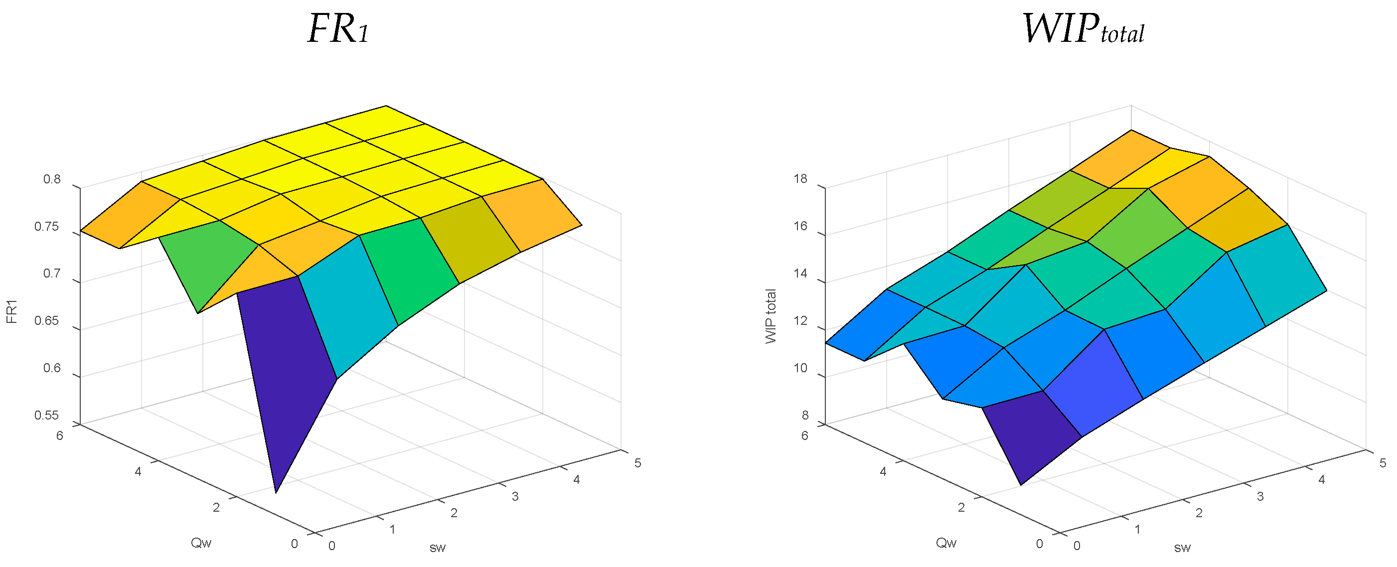
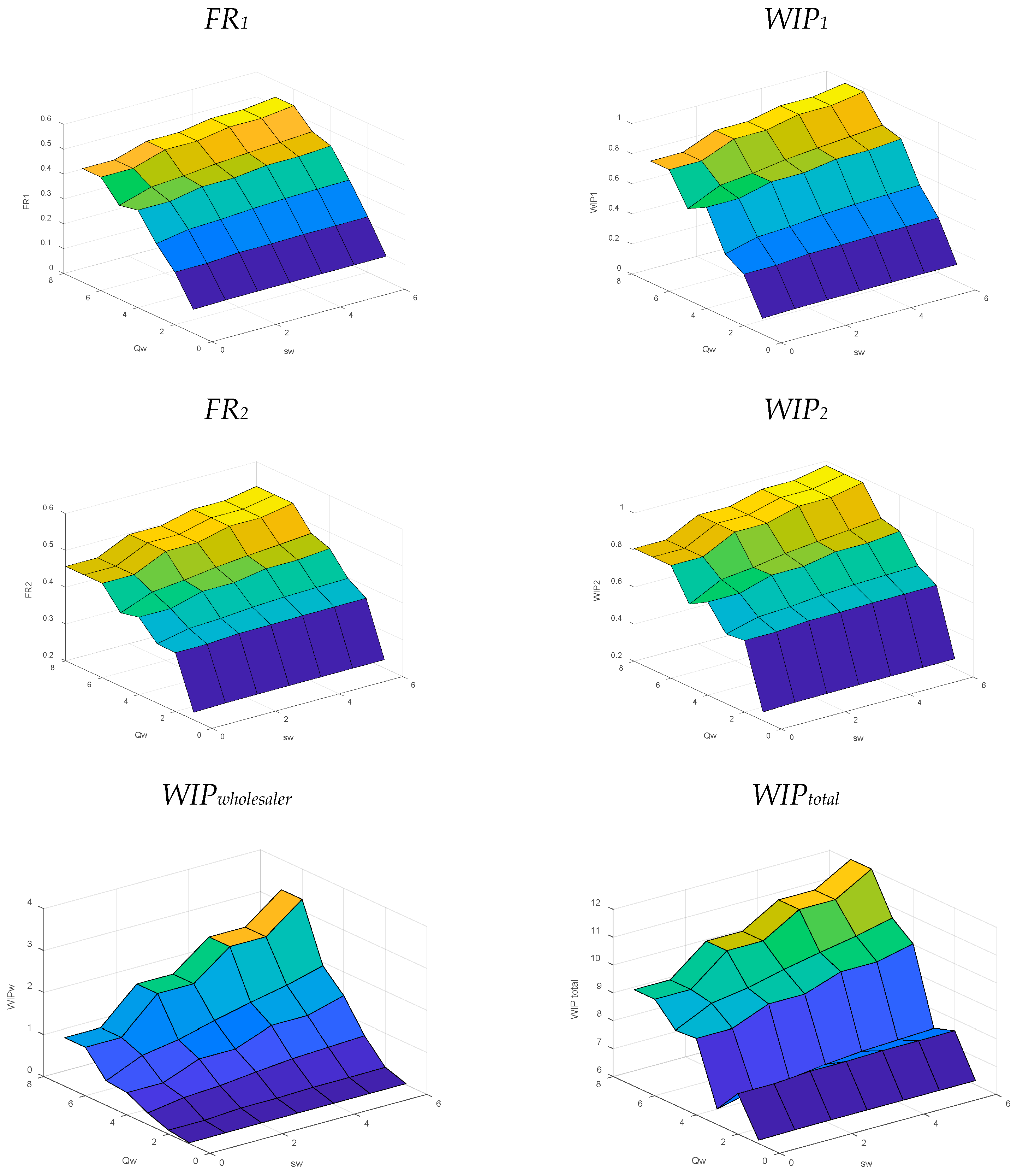
By increasing sw we can achieve better service levels at the retailers but again at the cost of an increase in the average total inventory (Figure 9). The effect of Qw is less straightforward. In general, fill rates at the retailers and the average total inventory tend to increase with increasing Qw, but jagged patterns may be observed (Figure 10). There is strong interplay between the parameters, and for certain scenarios it is actually possible to enhance retailers’ performance, while actually decreasing the average inventory in the system (Figure 11). The presence of some safety stock at the wholesaler (sw > 0) can protect the retailers from significant deviations in fill rates (Figure 12). The effect of the wholesaler’s policy on both retailers is similar.

5.1.3. Retailers’ Policy (si, Qi) for Balanced Systems

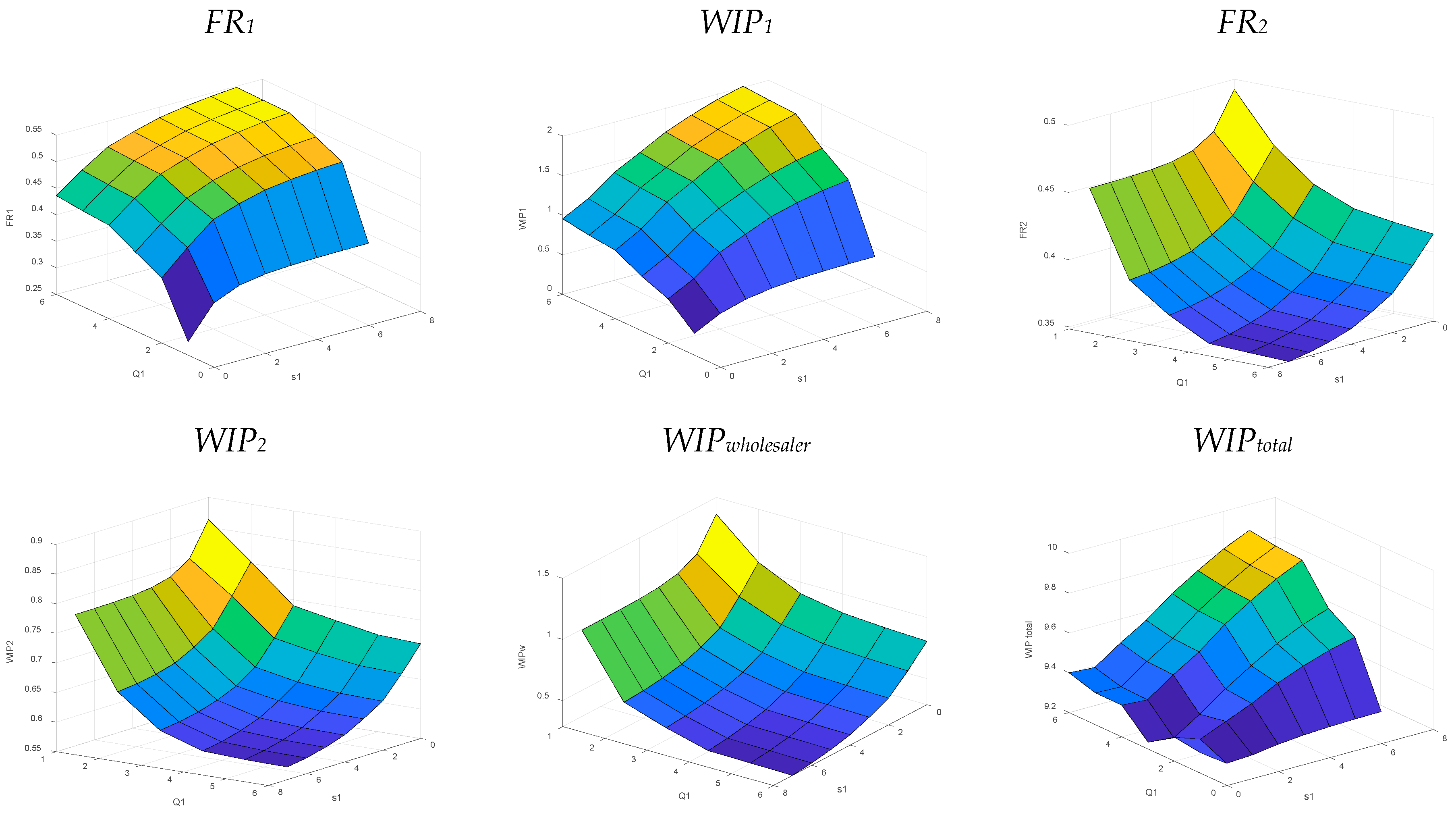
Increasing si causes an increase in the fill rate at retailer i but also an increase in the average inventory at retailer i. Although both average inventory at the DC and average inventory at the wholesaler is negatively correlated with si, the overall effect on WIPtotal is a clear increase. Up to a point, increasing the reorder point at retailer i causes a transfer of available inventory downstream. This has a negative effect on the performance of the other retailers (Figure 13).
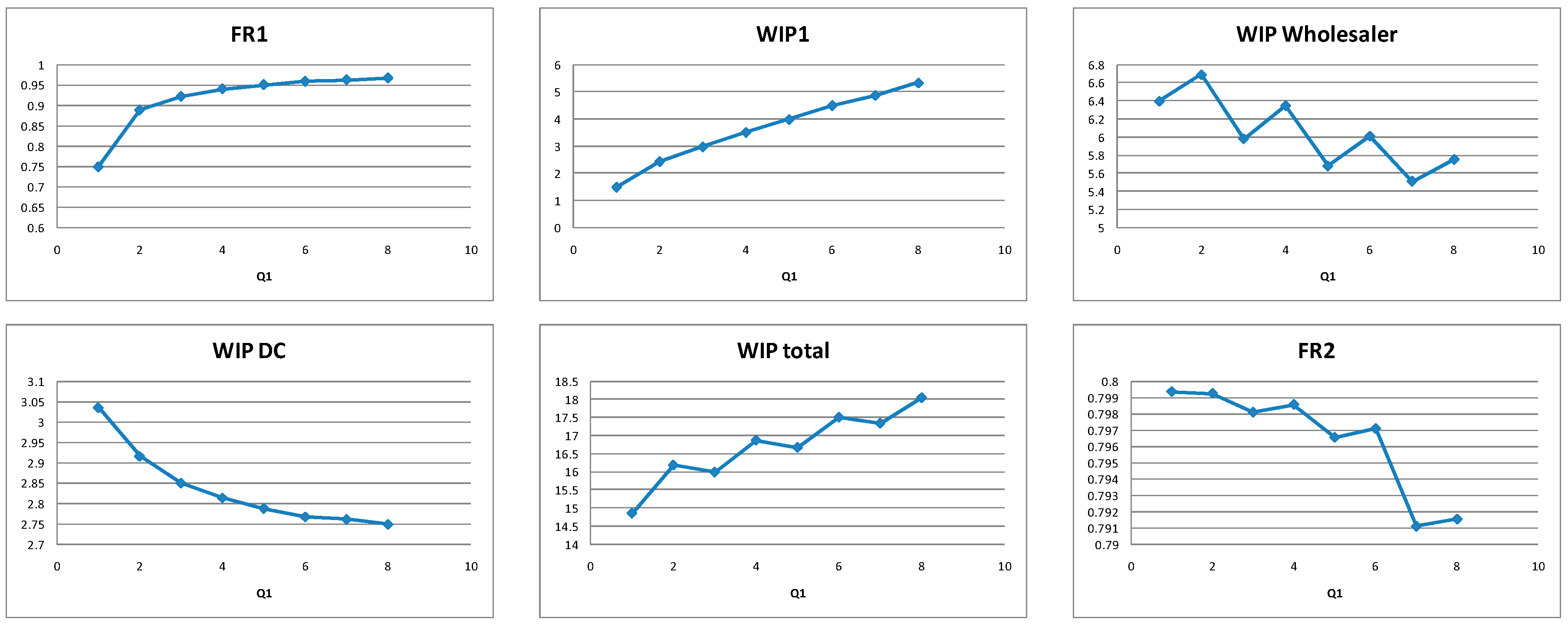
Similarly, an increase in Qi increases both the fill rate and average inventory at retailer i. The effect on the wholesaler’s average inventory is more dynamic. In general, WIP wholesaler tends to decrease with an increasing Qi, but saw-like patterns can also be observed (Figure 14). Average inventory at the distribution center decreases with Qi. The average total inventory in the system is generally positively correlated with Qi, but due to the WIPwholesaler contribution, a jagged pattern may be observed. As was the case with si, the increase in Qi causes a downstream transfer of available inventory, and this has a negative effect on the performance of the other retailers. The managerial implication of the dynamic system behavior is that there are good reasons for the fine-tuning of the system. Small changes in inventory policies may achieve an enhanced performance in terms of both customer satisfaction and total system inventory.

5.2. The Effect of Policy Parameters—Supply-Constrained Systems

We investigate supply-constrained systems where λ 1 = λ 2 > μ 1 = μ 2 > μ w > μ d . For the numerical examples that follow, the parameters were λ1 = λ2 = 3, μ1 = μ2 = 2, μw = 1, and μd = 0.8.

5.2.1. Distribution Center’s Policy (sd, Qd) for Supply Constrained Systems

Compared to balanced systems, in supply-constrained systems the retailers are more sensitive to DC policy changes. In general the reorder quantity Qd has a greater effect on the performance measures than sd (Figure 15). Jagged patterns may also be observed, so attention should be given to fine-tuning the system.

5.2.2. Wholesaler’s Policy (sw, Qw) for Supply Constrained Systems

Again, supply-constrained systems are more sensitive to design variable changes. In general the effect of reorder quantity Qw is more important than that of sw, while jagged patterns in the performance measures may also occur. The wholesaler’s policy can be an effective way to enhance retailers’ performance. Higher sw and Qw values lead to higher availability of products at the wholesaler and a better service for the retailers. This causes an increase in average inventories not only at the wholesaler but also downstream at the retailers (Figure 16).

5.2.3. Retailers’ Policy (si, Qi) for Supply Constrained Systems

As with balanced systems, increasing si or Qi causes a transfer of available inventory downstream, and the fill rate at retailer i increases. In general, total inventory increases, but in some scenarios a small decrease in WIPtotal may be initially observed (Figure 17). Compared to balanced systems, changing the policy of one retailer has a greater impact on the performance of the other retailers.

5.3. The Effect of Number of Retailers

Each retailer acts independently from the others, and no demand correlation is assumed. However, since all retailers are supplied by a finite-capacity wholesaler, some interaction amongst them occurs. We study a system with three retailers, and we focus on how the inventory policy of one retailer affects the performance of the others. We focus on the retailer with the highest (retailer 3) and the lowest (retailer 1) priority. For the following examples we assume for the balanced systems μ1 = μ2 = μ3 = λ1 = λ2 = λ3 = μw/3 = μd/3, and for the supply-constrained systems λ1 = λ2 = λ3 = 3, μ1 = μ2 = μ3 = 2, μw = 1, and μd = 0.8.

5.3.1. Interactions Between the Retailers

Changing the reorder point si causes small (sometimes insignificant) but consistent decreases in the performance of the other retailers (Figure 18 and Figure 19).
Parameter Q directly affects the availability of inventory at the wholesaler, and thus the ability of the wholesaler to respond to demand from the other retailers, so greater effects are observed (Figure 20 and Figure 21). For balanced systems, in some scenarios an increase in Q in one retailer caused small increases in fill rates in two or more retailers (Figure 20). Such cases indicate the coordination between the inventory policies of the various network members and are of interest from a managerial point of view.
The lowest priority retailers were found to be more sensitive to changes in the other retailers’ policies.

5.3.2. The Effect of Retailer Addition

We investigate the behavior of the system with an increasing number of retailers supplied by the same wholesaler. All retailers are assumed to follow the same inventory control policy, while replenishment times are also the same for all retailers.
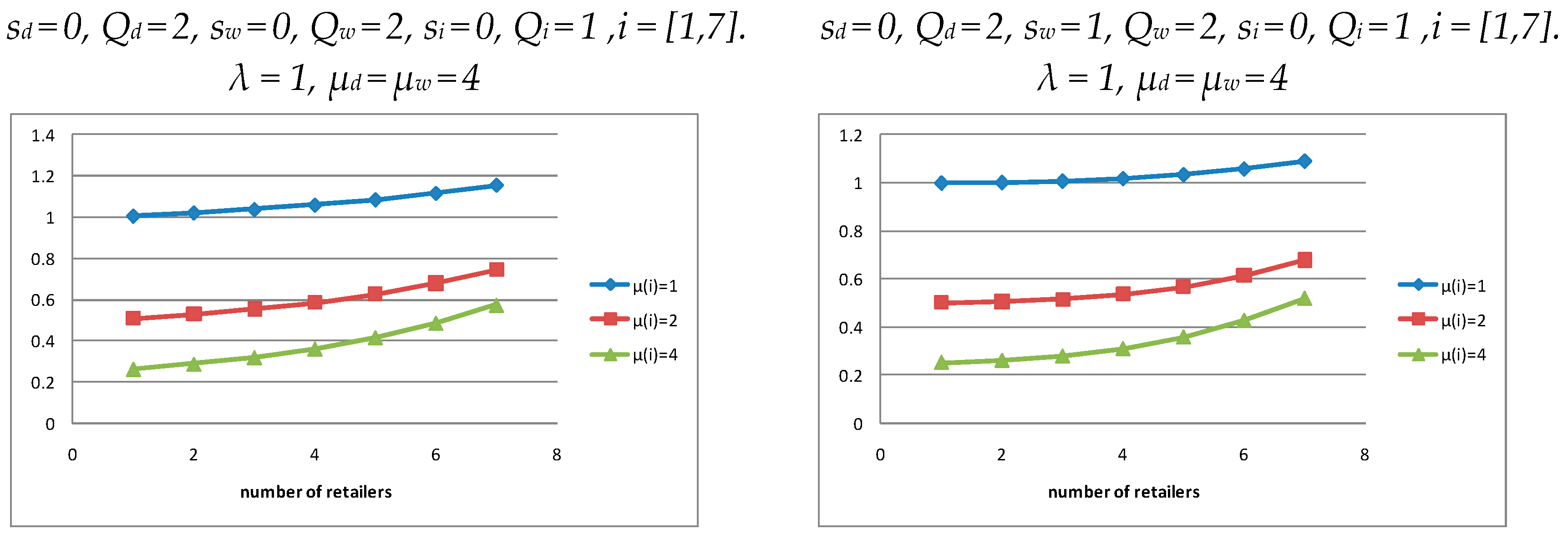
Increasing the number of retailers causes the fill rates to decrease as the available inventory at the wholesaler decreases. Initially, the effect is almost the same for all retailers, irrespective of their designated priority. Beyond a point the antagonism between the retailers becomes more intense as the stock-out probability for the wholesaler becomes important and priorities start to have an effect on retailers’ performance (Figure 22).
Considering total system performance, by increasing the number of retailers we increase the total output, but at the same time total lost sales also increase. The ratio of lost sales to output increases with n. The changes in the ratio depend on the other parameters of the system as well, and they are more important for higher retailer transportation rates (Figure 23). The optimal number of retailers will depend on the specific costs parameters.

6. Conclusions

In this paper we presented a model based on continuous time discrete space Markov processes for the exact numerical analysis of a single-product, three-echelon inventory system with multiple retailers. A solution algorithm based on the properties of the infinitesimal generator matrix was developed, and the model was used to investigate the effect of the decision variables on the performance measures of the system. The algorithm was validated by comparing the results with simulation, and for all cases there was a very good agreement.
Conclusions were drawn based on extensive numerical research on different scenarios for balanced and supply-constrained systems. The results indicate a dynamic behavior. There is interdependence between the different members of the network and interplay between system parameters. More importantly from a managerial point of view, our analysis also indicates that in some cases it is possible to coordinate the system, increasing customer satisfaction (fill rates), while at the same time decreasing average total inventory in the network. For balanced systems some safety stock was found to be desirable at both the DC and the wholesaler, while the possibility of coordination of the supply network members could be explored by fine-tuning either the wholesaler’s or the retailers’ policies. In regard to supply-constrained systems, DC and wholesaler policies were found to be more important for overall system performance, while the effect of each retailer’s policy on the performance of the others was also stronger.
The novelty of our approach in comparison to previous three-echelon models is the following:
  • Our model provides an exact analytical solution for the examined system in contrast with other three-echelon models where approximation methods are used.
  • The exact Markov chain solution in this paper can reveal important properties and the general behavior of the system that cannot be identified when approximation techniques are used.
  • Beyond its theoretical contribution, the model serves as a benchmarking tool for simulation and heuristic methods, thereby providing both methodological rigor and actionable managerial guidance.
As further research, four directions are proposed. Regarding external demand, more general demand distributions can be investigated. Although the Poisson distribution is commonly used to model demand in inventory systems, it may not be appropriate to describe more complex and more realistic cases. A compound Poisson distribution combining Poisson arrivals for customers with an empirical distribution for individual demand would offer more modeling flexibility, and it would be relatively easy to integrate in the presented model. In a second direction, more general distributions can be used for replenishment times. The application of phase-type distributions (Erlang, Coxian) to model times would allow for more realistic modeling, but it must be kept in mind that the total number of states, and so the computing requirements, would increase. In a third direction, such a model may be used as a decomposition block for the analysis of larger systems using approximate methods like decomposition, aggregation techniques, etc. Finally, the development of a cost function would allow the model to be used for optimization purposes. This could be achieved either through an exhaustive enumeration of possible policies or by combining the evaluative algorithm with an optimization heuristic.

Author Contributions

Conceptualization, G.V., S.K., A.D. and E.I.; methodology, G.V., S.K., A.D. and E.I.; software, G.V., S.K., A.D. and E.I.; validation, G.V., S.K., A.D. and E.I.; formal analysis, G.V., S.K., A.D. and E.I.; investigation, G.V., S.K., A.D. and E.I.; resources, G.V., S.K., A.D. and E.I.; data curation, G.V., S.K., A.D. and E.I.; writing—original draft preparation, G.V., S.K., A.D. and E.I. All authors have read and agreed to the published version of the manuscript.

Funding

This research received no external funding.

Data Availability Statement

The original contributions presented in this study are included in the article. Further inquiries can be directed to the corresponding author.

Conflicts of Interest

The authors declare no conflict of interest.

References

  1. Axsäter, S. Inventory Control; International Series in Operations Research & Management Science 225; Springer International Publishing: Cham, Switzerland, 2015; pp. 191–222. [Google Scholar]
  2. Agrawal, N.; Smith, S.A. Multi-location Inventory Models for Retail Supply Chain Management—A Review of Recent Research. In Retail Supply Chain Management; Agrawal, N., Smith, S.A., Eds.; International Series in Operations Research & Management Science 223; Springer: Berlin/Heidelberg, Germany, 2009; pp. 319–347. Available online: https://link.springer.com/book/10.1007/978-0-387-78902-6 (accessed on 22 September 2025).
  3. Rofman, E.; González, R.; Sagastizábal, C. Global Optimization of Arborescent Multilevel Inventory Systems. J. Glob. Optim. 1995, 6, 269–292. [Google Scholar] [CrossRef]
  4. Ahire, S.L.; Schmidt, C.P. A model for a Mixed Continuous-Periodic Review One-Warehouse, N-Retailer inventory system. Eur. J. Oper. Res. 1996, 92, 69–82. [Google Scholar] [CrossRef]
  5. Yang, P.; Wee, H. An arborescent inventory model in a supply chain system. Prod. Plan. Control 2001, 12, 728–735. [Google Scholar] [CrossRef]
  6. Abdul-Jalbar, B.; Gutiérrez, J.M.; Sicilia, J. Single cycle policies for the one-warehouse N-retailer inventory/distribution system. Omega 2006, 34, 196–208. [Google Scholar] [CrossRef]
  7. Yao, M.J.; Wang, Y. A new algorithm for one-warehouse multi-retailer systems under stationary nested policy. Optim. Methods Softw. 2006, 21, 41–56. [Google Scholar]
  8. Lagodimos, A.; Koukoumialos, S. Service performance of two-echelon supply chains under linear rationing. Int. J. Prod. Econ. 2008, 112, 869–884. [Google Scholar] [CrossRef]
  9. Hsiao, Y.-C. Optimal single-cycle policies for the one-warehouse multi-retailer inventory/distribution system. Int. J. Prod. Econ. 2008, 114, 219–229. [Google Scholar] [CrossRef]
  10. Abdul-Jalbar, B.; Segerstedt, A.; Sicilia, J.; Nilsson, A. A new heuristic to solve the one-warehouse N-retailer problem. Comput. Oper. Res. 2010, 37, 265–272. [Google Scholar] [CrossRef]
  11. Geng, W.; Qiu, M.; Zhao, X. An inventory system with single distributor and multiple retailers: Operating scenarios and performance comparison. Int. J. Prod. Econ. 2010, 128, 434–444. [Google Scholar] [CrossRef]
  12. Helper, C.M.; Davis, L.B.; Wei, W. Impact of demand correlation and information sharing in a capacity constrained supply chain with multiple-retailers. Comput. Ind. Eng. 2010, 59, 552–560. [Google Scholar] [CrossRef]
  13. Panda, D.; Maiti, M.K.; Maiti, M. Two warehouse inventory models for single vendor multiple retailers with price and stock dependent demand. Appl. Math. Model. 2010, 34, 3571–3585. [Google Scholar] [CrossRef]
  14. Paul, B.; Rajendran, C. Rationing mechanisms and inventory control-policy parameters for a divergent supply chain operating with lost sales and costs of review. Comput. Oper. Res. 2011, 38, 1117–1130. [Google Scholar] [CrossRef]
  15. Guan, R.; Zhao, X. Pricing and inventory management in a system with multiple competing retailers under (r, Q) policies. Comput. Oper. Res. 2011, 38, 1294–1304. [Google Scholar] [CrossRef]
  16. Solyalı, O.; Süral, H. The one-warehouse multi-retailer problem: Reformulation, classification, and computational results. Ann. Oper. Res. 2012, 196, 517–541. [Google Scholar] [CrossRef]
  17. Tempelmeier, H. A multi-level inventory system with a make-to-order supplier. Int. J. Prod. Res. 2013, 51, 6880–6890. [Google Scholar] [CrossRef]
  18. Wang, Q. A periodic-review inventory control policy for a two-level supply chain with multiple retailers and stochastic demand. Eur. J. Oper. Res. 2013, 230, 53–62. [Google Scholar] [CrossRef]
  19. Gayon, J.-P.; Massonnet, G.; Rapine, C.; Stauffer, G. Constant approximation algorithms for the one warehouse multiple retailers problem with backlog or lost-sales. Eur. J. Oper. Res. 2016, 250, 155–163. [Google Scholar] [CrossRef]
  20. Tayebi, H.; Haji, R.; Jeddi, B.G. Joint order (1, T) policy for a two-echelon, single-item, multi-retailer inventory system with Poisson demand. Comput. Ind. Eng. 2018, 119, 353–359. [Google Scholar] [CrossRef]
  21. John, K.; Rajendran, C.; Ziegler, H. A comparative study on allocation/rationing mechanisms operational with/without backorder clearing in divergent supply chains. Sadhana 2019, 44, 231. [Google Scholar] [CrossRef]
  22. Tsai, S.C.; Ho, I.-Y. Sample average approximation for a two-echelon inventory system with service-level constraints. J. Oper. Res. Soc. 2019, 70, 675–688. [Google Scholar] [CrossRef]
  23. Hoque, M.A. An optimal solution policy to an integrated manufacturer-retailers problem with normal distribution of lead times of delivering equal and unequal-sized batches. OPSEARCH 2021, 58, 483–512. [Google Scholar] [CrossRef]
  24. Najafnejhad, E.; Roodsari, M.T.; Sepahrom, S.; Jenabzadeh, M. A mathematical inventory model for a single-vendor multi-retailer supply chain based on the Vendor Management Inventory Policy. Int. J. Syst. Assur. Eng. Manag. 2021, 12, 579–586. [Google Scholar] [CrossRef]
  25. Kurian, J.; Brijesh, P.; Chandrasekharan, R.; Ziegler, H. Priority fractional rationing (PFR) policy and a hybrid metaheuristic for managing stock in divergent supply chains. Sådhanå 2022, 47, 254. [Google Scholar]
  26. Lu, C.-J.; Gu, M.; Lee, T.-S.; Yang, C.-T. Integrated multistage supply chain inventory model of multiple retailers with imperfect production and inspection systems. Soft Comput. 2022, 26, 12057–12075. [Google Scholar] [CrossRef]
  27. Smirnov, D.; Herer, Y.T.; Avrahami, A. The continuous delayed distribution problem. Comput. Oper. Res. 2022, 148, 105976. [Google Scholar] [CrossRef]
  28. Andersson, J.; Malmberg, F.; Marklund, J. Exact analysis of One-Warehouse-Multiple-Retailer inventory systems with quantity restricted deliveries. Eur. J. Oper. Res. 2023, 309, 1161–1172. [Google Scholar] [CrossRef]
  29. Wang, Q.; Wan, G. Fixed-interval order-up-to policies and myopic optimal warehouse stock allocation for one-warehouse multiple-retailer systems. Eur. J. Oper. Res. 2023, 309, 1112–1124. [Google Scholar] [CrossRef]
  30. Kaynov, I.; van Knippenberg, M.; Menkovski, V.; van Breemen, A.; van Jaarsveld, W. Deep Reinforcement Learning for One-Warehouse Multi-Retailer inventory management. Int. J. Prod. Econ. 2024, 267, 109088. [Google Scholar] [CrossRef]
  31. Stranieri, F.; Fadda, E.; Stella, F. Combining deep reinforcement learning and multi-stage stochastic programming to address the supply chain inventory management problem. Int. J. Prod. Econ. 2024, 268, 109099. [Google Scholar] [CrossRef]
  32. Wu, Y.; Cheng, T.C.E.; Zhang, J. A serial mixed produce-to-order and produce-in-advance inventory model with multiple retailers. Int. J. Prod. Econ. 2012, 136, 378–383. [Google Scholar] [CrossRef]
  33. Islam, S.S.; Hoque, A.; Hamzah, N. Single-supplier single-manufacturer multi-retailer consignment policy for retailers’ generalized demand distributions. Int. J. Prod. Econ. 2017, 184, 157–167. [Google Scholar] [CrossRef]
  34. Stauffer, G. Approximation algorithms for k-echelon extensions of the one warehouse multi-retailer problem. Math. Methods Oper. Res. 2018, 88, 445–473. [Google Scholar] [CrossRef]
  35. Gruson, M.; Bazrafshan, M.; Cordeau, J.-F.; Jans, R. A comparison of formulations for a three-level lot sizing and replenishment problem with a distribution structure. Comput. Oper. Res. 2019, 111, 297–310. [Google Scholar] [CrossRef]
  36. Gruson, M.; Cordeau, J.-F.; Jans, R. Split demand and deliveries in an integrated three-level lot sizing and replenishment problem. Comput. Oper. Res. 2024, 161, 106434. [Google Scholar] [CrossRef]
  37. Cunha, J.O.; Melo, R.A. Valid inequalities, preprocessing, and an effective heuristic for the uncapacitated three-level lot-sizing and replenishment problem with a distribution structure. Eur. J. Oper. Res. 2021, 295, 874–892. [Google Scholar] [CrossRef]
  38. Gharaei, A.; Amjadian, A.; Shavandi, A. An integrated reliable four-level supply chain with multi-stage products under shortage and stochastic constraints. Int. J. Syst. Sci. Oper. Logist. 2023, 10, 1958023. [Google Scholar] [CrossRef]
  39. Geevers, K.; van Hezewijk, L.; Mes, M.R.K. Multi-echelon inventory optimization using deep reinforcement learning. Central Eur. J. Oper. Res. 2023, 32, 653–683. [Google Scholar] [CrossRef]
  40. Lin, H.; Lin, J.; Wang, F. An innovative machine learning model for supply chain management. J. Innov. Knowl. 2022, 7, 100276. [Google Scholar] [CrossRef]
  41. Blancas-Rivera, R.; Cruz-Suárez, H.; Portillo-Ramírez, G.; López-Ríos, R. $(s, S)$ Inventory policies for stochastic controlled system of Lindley-type with lost-sales. AIMS Math. 2023, 8, 19546–19565. [Google Scholar] [CrossRef]
  42. Akbari, M.; Do, T.N.A. A systematic review of machine learning in logistics and supply chain management: Current trends and future directions. Benchmarking Int. J. 2021, 28, 2977–3005. [Google Scholar] [CrossRef]
  43. Bijvank, M.; Vis, I.F. Lost-sales inventory theory: A review. Eur. J. Oper. Res. 2011, 215, 1–13. [Google Scholar] [CrossRef]
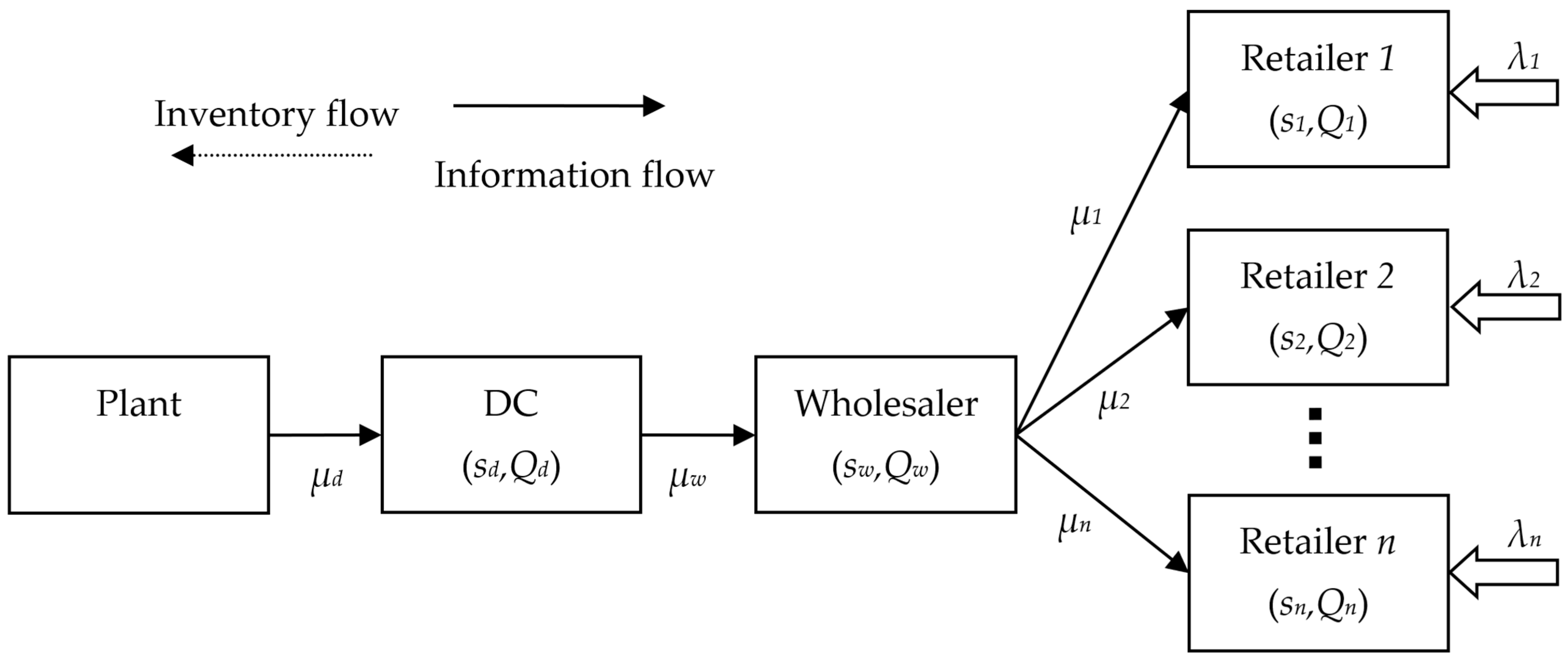
Figure 1. System layout.
Mathematics 13 03199 g001
Figure 2. The submatrices of block C1.
Mathematics 13 03199 g002
Figure 3. The submatrices of block C2.
Mathematics 13 03199 g003
Figure 4. The submatrices of block Ci.
Mathematics 13 03199 g004
Figure 5. % deviation (100 × (analytic-simulation)/analytic) between algorithmic solution and simulation results for a system with five retailers, sd = {2,4}, Qd = 2, sw = 0, Qw = 2, s1 = 0, Q1 = 1, s2 = 1, Q2 = 1, s3 = 0, Q3 = {1,2}, s4 = 0, Q4 = {1,2}, 0 ≤ s5 ≤ 3, 1 ≤ Q5 ≤ 2 and parameters μd = 2.5, μw = 3.6, μ1 = 1, μ2 = 1.2, μ3 = 1.4, μ4 = 1.6, μ5 = 1.8, λ1 = 0.5, λ2 = 0.7, λ3 = 0.9, λ4 = 1.2, λ5 = 1.5. Simulation parameters: one replication of 2,000,000 time units with a warm up period of 10,000 time units.
Mathematics 13 03199 g005
Figure 6. The effect of sd on system performance measures; Qd = 2, sw = 2, Qw = 1, s1 = 1, Q1 = 2, s2 = 1, Q2 = 1.
Mathematics 13 03199 g006
Figure 7. The effect of Qd on system performance measures: sd = 2, sw = 2, Qw = 2, s1 = 1, Q1 = 2, s2 = 1, Q2 = 2.
Mathematics 13 03199 g007
Figure 8. Compound effect of DC policy for Balanced Systems: sw = 2, Qw = 2, s1 = 2, Q1 = 3, s2 = 2, Q2 = 1.
Mathematics 13 03199 g008
Figure 9. The effect of sw on system performance measures: sd = 2, Qd = 2, Qw = 1, s1 = 1, Q1 = 2, s2 = 1, Q2 = 1.
Mathematics 13 03199 g009
Figure 10. The effect of Qw on system performance measures: sd = 4, Qd = 4, sw = 2, s1 = 1, Q1 = 2, s2 = 1, Q2 = 2.
Mathematics 13 03199 g010
Figure 11. Compound effect of wholesaler’s policy: sd = 2, Qd = 6, s1 = 1, Q1 = 2, s2 = 1, Q2 = 1.
Mathematics 13 03199 g011
Figure 12. Compound effect of wholesaler’s policy: sd = 3, Qd = 5, s1 = 1, Q1 = 2, s2 = 1, Q2 = 2.
Mathematics 13 03199 g012
Figure 13. The effect of s1 on system performance measures: sd = 4, Qd = 2, sw = 2, Qw = 4, Q1 = 2, s2 = 1, Q2 = 2.
Mathematics 13 03199 g013
Figure 14. The effect of Q1 on system performance measures: sd = 2, Qd = 2, sw = 6, Qw = 2, s1 = 2, s2 = 1, Q2 = 2.
Mathematics 13 03199 g014
Figure 15. Compound effect of DC policy for Supply Constrained Systems: sw = 2, Qw = 2, s1 = 2, Q1 = 3, s2 = 2, Q2 = 1.
Mathematics 13 03199 g015
Figure 16. Compound effect of wholesaler’s policy: sd = 2, Qd = 6, s1 = 1, Q1 = 2, s2 = 1, Q2 = 2.
Mathematics 13 03199 g016
Figure 17. Compound effect of retailer 1’s policy: sd = 2, Qd = 6, sw = 2, Qw = 4, s2 = 1, Q2 = 2.
Mathematics 13 03199 g017
Figure 18. Balanced system. Effect of s, sd = 0, Qd = 4, sw = 2, Qw = 4, si = 1, Qi = 2, μ1 = μ2 = μ3 = λ1 = λ2 = λ3 = μw/3 = μd/3.
Mathematics 13 03199 g018
Figure 19. Supply-constrained system. Effect of s, sd = 0, Qd = 4, sw = 2, Qw = 4, Q1 = 2, si = 1, Qi = 2λ1 = λ2 = λ3 > μ1 = μ2 = μ3 > μw > μd.
Mathematics 13 03199 g019
Figure 20. Balanced system. Effect of Q, sd = 0, Qd = 4, sw = 2, Qw = 4, si = 1, Qi = 2, μ1 = μ2 = μ3 = λ1 = λ2 = λ3 = μw/3 = μd/3.
Mathematics 13 03199 g020
Figure 21. Supply-constrained system. Effect of lowest priority retailer—Q, sd = 0, Qd = 4, sw = 2, Qw = 4, si = 1, Qi = 2, λ1 = λ2 = λ3 > μ1 = μ2 = μ3 > μw > μd.
Mathematics 13 03199 g021
Figure 22. Order fill rate of the highest and lowest priority retailers as a function of the number of retailers: sd = 0, Qd = 2, sw = 0, Qw = 2, si = 0, Qi = 1, i = [1,7]. λ = 1, μd = μw = 4.
Mathematics 13 03199 g022
Figure 23. Ratio of lost sales to output as a function of the number of retailers.
Mathematics 13 03199 g023
Disclaimer/Publisher’s Note: The statements, opinions and data contained in all publications are solely those of the individual author(s) and contributor(s) and not of MDPI and/or the editor(s). MDPI and/or the editor(s) disclaim responsibility for any injury to people or property resulting from any ideas, methods, instructions or products referred to in the content.