Abstract
The probability density function (PDF) of the product of two normal random variables remains an open discussion. Researchers have proposed many forms of PDFs. Among these, two notable PDFs are an analytical solution with infinite summation and an integral form with transformation. For practical computation, they must be estimated. The form with infinite summation must be truncated to a finite summation, and the form still in integration must be computed numerically. As a result of this estimation, an error occurs in the value of the estimation. This paper derives upper bounds for the estimation error resulting from truncation and numerical approximation in integral calculations. The upper bound error between the exact PDF and the truncated PDF is expressed as a geometric series using Bessel function inequality and Stirling’s approximation. The geometric formula allows the quantification of the total truncation error to be determined. For the PDF, which is still in integration form, the trapezoidal rule is used for numeric calculation. Hence, the error can be determined using the error-bound formula. The two estimated PDFs have their own advantages and disadvantages. The truncated PDF gives a relatively small upper bound value compared to the numerical calculation integral form PDF for a small value domain. However, the truncated PDF fails to perform for a large value domain, and only the integral form PDF can be used. The error for the estimation is applied to the conventional mass measurement. The results demonstrate that the error can be controlled through an analytical approach.
Keywords:
Bessel function; Stirling’s formula; dependent random variables; trapezoidal rule; bisection method MSC:
60E05; 62E17; 62P30
1. Introduction
The product of two random variables holds significant importance across various fields of study. In metrology, many random variable functions consist of the product of two random variables including the flow rate [1,2,3,4,5,6,7,8], electrical engineering [9,10,11], temperature measurement [12], conventional mass [13,14,15,16,17,18], and volume [19] measurement. In signal processing, it is used in radar and communication systems [20,21,22,23,24,25,26,27,28]. In risk management, a company’s cash flows are determined by the product of random variables, such as the output prices and exchange rates [29] and the output prices and volumes of sales [30]. Statistical distributions such as the PDF are essential elements for practical applications [20,21,22,23,24,25,26,27,28,29,30,31]. Among many distributions, the normal distribution is widely used to describe the random variables. Consequently, the PDF of the product of two normal distributions remains a topic of great interest.
The product of correlated normal random variables has been a subject of interest for more than 80 years [32]. In early studies, such as [33], the moment-generating function (MGF) was determined, but the product distribution itself remained unidentified [34]. The work of [33] was used by [35] to show that, when and are large, the product of two normal random variables approaches a normal distribution. It was not until 2016 that an exact PDF for the product of two correlated normal distributions was introduced in [20,36]. Specifically, ref. [36] provided the product of two correlated standard normal distributions, while [20] presented the general form of the PDF for distributions with arbitrary means and variances. In 2019, the product of two standard normal distributions in [36] was identified as the variance–gamma distribution in [37,38,39]. As for the product of two normal random variables with arbitrary means and variances, the distribution has yet to be identified.
Although the result in [20] has yet to be identified, it is a significant finding regarding the product of two normal random variables. The rigorous integral of the PDF is solved using the result in [40] with the modified Bessel function of the second order v within the solution. The result does come with advantages and disadvantages. The result is presented in a general form, encompassing other PDFs with specific parameter values. It is aligned with the results given in [36,41] (eq. 6.2, eq. 6.15, and eq. 6.28). However, the result in [20] is given in terms of an infinite summation because of the Taylor series of exponential expansion. In practical applications, this summation must be truncated at a sufficiently large integer value, resulting in an estimate of the PDF rather than the exact function.
While the product of two standard normal distributions can be clearly defined as a variance–gamma distribution, the product of two normal random variables is still open to discussion. Even with the analytical solution of the PDF given in [20], it must be truncated and can compensate for the resulting accuracy. Other research has used a variety of methods. In [34], the product distribution is estimated with an extended skew-normal (ESN) distribution. It shows that, in some cases, the ESN distribution produces an excellent estimation and performs better than the truncated PDF. Another research used an estimation of the PDF integral instead of a distribution approximation. In [42], the joint PDF is written by the marginal and copula functions. The PDF value is calculated by Monte-Carlo simulation based on the integration given in [43]. Even though the estimated PDFs give excellent results, the upper bound error of the estimation was not discussed.
In this paper, the first main contribution is an analytical derivation of the upper bound error function of the truncated PDF given in [20]. The upper bound error is the maximum difference between the true PDF and the truncated PDF. The difference is transformed into a convergent infinite geometric series summation using Stirling’s formula and the Bessel function inequality given in [44]. Hence, the summation result is a notable formula. The second contribution is the upper bound error for the numerical calculation of the PDF based on [42]. The numerical PDF is computed using the trapezoidal rule. Hence, the error bound formula is well-known for the numerical calculation of integrals. The third contribution is a proposed algorithm to accompany the upper bound error in numerical calculations. The algorithm is a combination of modified Markov Chain Monte Carlo (MCMC) and the bisection method. Finally, we applied the results to a practical computation of conventional mass measurement. The data used in this practical application are actual data taken from the Mass Laboratory, Ministry of Trade. The observed data allow testing the performance of the estimated PDFs and their upper bound errors in real-world applications.
The remainder of this paper is structured as follows. Section 2 defines the estimated PDF. Section 3 presents the main result: an upper bound for the estimation error. Section 4 evaluates the proposed method through numerical simulations in MATLAB R2022a. Section 5 presents the application upper bound in conventional mass measurement. Finally, Section 6 provides concluding remarks.
2. Estimated Probability Density Function
Before the findings of [20] were presented, various PDFs were used based on specified parameters. For instance, the PDF given in [41] (eq. 6.2 and eq. 6.15) can be used for the product of two normal random variables with means equal to zero and arbitrary variance. The result in [36] can be used only for the product of two standard normally distributed random variables. In the case of independent random variables, where one mean equals zero and both have identical variances, the function provided in [41] (eq. 6.28) can be used.
The PDF given in [20] is in a general form such that it can handle all of the specific parameters. It is more convenient to use only one general function instead of many functions that require specific parameters. The parameters of two random variables can be arbitrary, i.e., and with . The random variables can be written in bivariate normal distribution in the following theorem of the exact PDF of the product of two normal random variables , which is given by the following:
Theorem 1
([20]). Let . Then, the exact PDF, , of the product is given by
where is the absolute value operation, is the modified Bessel function of the second kind order v, and is a sign function.
One property of the modified Bessel function that is essential to compute the PDF value is . This property can be shown by the relationship of the modified Bessel function of the second kind with the first kind given in [45]:
The exact PDF given above consists of an infinite summation. In practice, however, infinite summation cannot be used for calculation. To calculate the value, the infinite summation is replaced by an integer. The estimated PDF with finite summation is called the truncated PDF, and it is also introduced for numerical computation in this article. It is also shown in this article that the truncated PDF gives a reasonable estimation, even with a small number of summations. However, to the authors’ knowledge, the upper bound error function of using the truncated PDF has yet to be intensively discussed. Solving the upper bound error analytically is one of the primary purposes of this paper.
The truncated PDF in [20] is similar to the exact PDF given in (1), except that the summation to infinity is replaced by an integer. It is given in notation , where k is an integer that replaces infinity in the calculation. Because of the integer replacement of infinity, the truncated PDF will have an error. In order to increase the accuracy of the truncated PDF value computation, the k-length summation is made as large as possible. Since the k-length summation will determine the error of the truncated PDF, it is important to determine the k-length summation that complies with the permissible error requirement.
While [20] focuses on solving the integration given in [43] for the product of two random variables, the PDF given in [42] transforms the integration using the copula function. Using the copula function, the joint PDF can be written in terms of the marginal PDF. The interval of the integral can be transformed from 0 to 1 for any distribution. The PDF and cumulative distribution function (CDF) given in [42] for the product of two arbitrary distribution random variables is given by
Theorem 2
([42]). Let be a vector of two continuous random variables with marginal distributions and , respectively. Let C be the copula modeling the dependence of the random vector (X,Y) then the PDF and CDF of the random variable are given by
where is the inverse function of , and c denotes the density of copula C.
The CDF and PDF for the product of two normal distribution random variables are given by using (3). The PDF and the CDF of the product of two normal distributions are given by the following corollary:
Corollary 1.
Let . Then, the PDF, , and the CDF, , of the product are given by
where ϕ and Φ are the PDF and CDF of the standard normal distribution, respectively, and denotes the inverse function of .
Proof.
The proof follows [46], where the PDF is determined for the quotient of two normal random variables.
The proof starts with the CDF
and is given in [47] as
by substituting (5) and (7) into (3), we have
By taking the derivative with respect to w, we have
□
The PDF estimation in [42] is the numeric integral of (4). The integral is calculated by the trapezoidal rule, given as
where
and , j = 1, 2, 3, …, n.
The CDF estimation in [42] is the numeric integral of (4). The integral is calculated by the trapezoidal rule, given as
where
and , j = 1, 2, 3, …, n.
While the estimated PDF in [20,42] is based on the integration of [43], an earlier approach is based on the MGF of a random variable W. The PDF is estimated as a normal distribution when , and ; when , the Type III function and the Gram–Charlier Type A series can be used to estimate the PDF of the product of two normal random variables [35]. When the requirement of the seems to qualify, the random variable is estimated by , where and is given by
The mean and variance given above are from [34]. However, the results assume that in [34] the random variable is written as . The MGF of the random variable is given in [33] as
Both estimated PDFs have their advantages and disadvantages. The benchmark can be determined by the upper bound error, calculation methods, and computation time. The comparison between the estimated PDF of and and the exact PDF is given in the next section.
3. The Upper Bound Error of the Estimated Probability Density Function
3.1. The Upper Bound Error of the Truncated Probability Density Function
The upper bound error of the truncated PDF, , at each point is given by the following proposition:
Proposition 1.
Let . Suppose the exact PDF and the truncation k-length PDF of the random variable are denoted by and , respectively. If the remainder of the difference is , then
where
and
where k is an integer sufficiently large, such that .
Proof of Proposition 1.
The proof requires Stirling’s formula and Lemma 1 [44].
Stirling’s formula is used to find the upper bound of the factorial of an integer. Stirling’s formula is given by [48,49] as
Lemma 1 ([44])
Let be the modified Bessel function of second kind order v; then,
for and .
Lemma 1 is used to determine the upper bound of the modified Bessel function. By Lemma 1, the upper bound of the modified Bessel function can be written in . Since , Lemma 1 can be written as
By (19), we have
Proof.
The inequality of (20) can be shown by induction.
- Base case, :The inequality above is true by (19).
- Induction hypothesis:
- Induction Step:By Lemma 1, we haveUsing the induction hypothesis, we have
□
Since , and ; therefore, (23) can be written as
The remainder is the subtraction between the exact and the truncated PDF, which is given by
The core of the proof is to express the upper bound of in terms of an infinite geometric series summation. Hence, by converting the bound to a geometric series, we can find the infinite summation. Lemma 1 allows the modified Bessel function of the second kind to be written in order zero and eliminates the effect of the infinite summation of the order of the Bessel function. For the factorial in , Stirling’s formula is used as an upper bound, allowing the factorial to be written in terms of powers and multiplication. The proof starts with using the result of Lemma 1, substituting (24) into (25) with . Hence, the remainder of the true PDF and truncated PDF is less than or equal to the following:
by rewriting variables with the power of n and m, we have
and by binomial theorem, (27) can be written as
By extracting the power of n in (28), we have
and using Stirling’s formula, we can find a function that is greater than (29) as follows:
By extracting the power of n, we have
The summation in (31) becomes a geometric series summation. Since , when , we have
By substituting (32) into (31), we have
and let k be a positive integer with a sufficiently large value to produce . The summation in (33) becomes a convergent infinite geometric series summation and can be written as
Therefore, equation (33) can be written as
□
The expression in (35) is a function of the upper bound error at each point of the truncated PDF in [20]. Since the result of (35) is based on the geometric sum formula, the proposition can only be used when . The integer k must be chosen so that r meets the requirement. Hence, the parameter values influence the minimum number of k. While the upper bound for the truncated PDF in [20] is determined by an analytical approach, the PDF estimation of [42] is determined by analytic and numeric approaches.
3.2. The Upper Bound of the Trapezoidal Calculation of the Probability Density Function
The upper bound error for the trapezoidal rule is a well-known formula. The challenge when using the formula is finding the second derivative of the integration function. The next step is to find the maximum of the second derivative. The integration function of the PDF of the product of two normal random variables is given by
Hence, the upper bound error of the trapezoidal rule is given by
where for . The second derivative of with respect to u is rigorous if conducted by hand. The derivative can be acquired using Maple 2025 using the substitution for as the input for the derivative. The notation is used as a dummy to replace the inverse CDF of the standard normal distribution. The derivative can be obtain by manually by substituting and in the Maple result. Since it is difficult to solve for t that meets , the value of t that maximizes is computed numerically using the proposed method.
The proposed method for calculating the upper bound error is a modified MCMC approach combined with the bisection. The modified MCMC uses the same concept of a random generator; however, the modified algorithm uses a normal distribution instead of a uniform distribution. The random number is generated from a normal distribution; the point that has the highest value within the function will be the mean of the next random generator. This procedure allows the previous point as a consideration for a more focused area of the random generator and minimizes the chance of a local maximum result. The result of this algorithm is then sent to the bisection search for further refining the result. The algorithm and flowchart for the modified MCMC with a combination of bisection search are given in Algorithm 1 and Figure 1, respectively.
| Algorithm 1 Modified MCMC and Bisection Refinement |
|
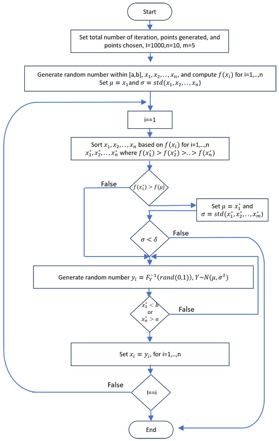
Figure 1.
Flowchart of the proposed algorithm combining modified MCMC and bisection algorithm.
In a practical situation for computing the PDF, the upper bound error may be determined beforehand. The minimum values of k and n are of interest. We can write it in general terms as follows:
where is the predetermined upper bound error. While the analytical solution of finding k and n is challenging to solve, they can be determined using Algorithms 2 and 3.
| Algorithm 2 Find minimal k such that and over a grid of w |
|
| Algorithm 3 Find minimal n such that over a grid of w |
|
In order to observe the performance of the estimated PDF, values must be assigned to the parameters. In the next section, the upper bound error is examined using predetermined parameters.
4. Numerical Results
The upper bound error of and is inspected based on the parameters given in [20,50]. The upper bound error of the truncated function, , is shown by , while the upper bound error for the trapezoidal numeric integration, , is shown by .
Proposition 1 is inspected using zero and nonzero mean parameters. The parameters chosen from [20,50] are intended to analyze the proposition. The parameter separation contributed to the existing PDF of zero means derived from solving analytically. In contrast, for nonzero means, numerical results are the only option to investigate the error of the truncated PDF.
Using parameters of means equal to zero with independent and dependent correlation should comply with the result in [36,41]. The PDF of two dependent normally distributed random variables with means equal to zero in [36,41] is given by
For both cases of dependence with means equal to zero, Proposition 1 gives , and since , the upper bound error is equal to zero, . The result shows that, if the means are equal to zero, then the PDF given in [20] provides an exact function, not the estimation. Hence, the result complies with Proposition 1. The proposition also complies with the undefined value of the exact and the truncated PDF when . The modified Bessel function of the second kind has an undefined value when ; hence, the upper bound error also gives an undefined value. In software computation, point is excluded by adding code.
For a nonzero mean, the parameters chosen in [20] are (Figure 2) and (Figure 3). The value of satisfies the requirement of for the chosen parameters. The upper bound error function is given in dB as
The upper bound error transformation in terms of dB is used to plot different plots with different parameters in one figure.
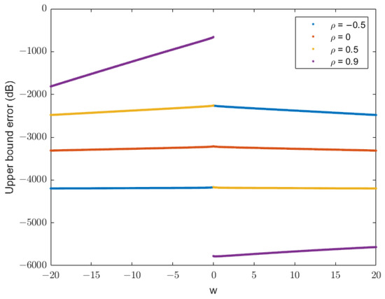
Figure 2.
Plot of the upper bound error function in dB for , , , , and . The plot shows how the upper bound error varies across w for different correlation coefficients (). Higher correlations () tend to increase the upper bound error.
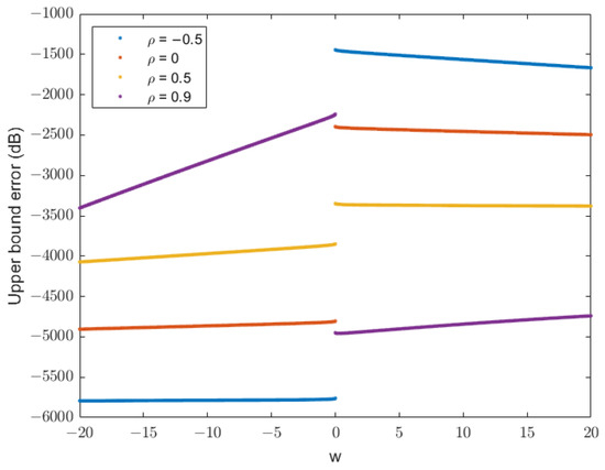
Figure 3.
Plot of the upper bound error function in dB for , , , , and . The plot illustrates the variation of the upper bound error across w for different correlation coefficients (), showing the impact of both correlation and mean values on the truncation error.
Other sets of parameters are chosen from [50] are , (Figure 4) and , (Figure 5).With the increasing number of summation k, the smaller the difference between the Monte-Carlo simulation and truncated PDF in [20] is. The truncated PDF is called the Cui et al. approach in [50]. By Proposition 1, the upper bound errors are shown in Figure 6 and Figure 7. The errors peak for ; this might be the cause of the modified Bessel function of the second kind diverging to infinity at zero. The same condition also occurs for the parameters given in [20]. While the PDF does not give a value at exactly , the PDF shows a reasonable estimation of the exact PDF.
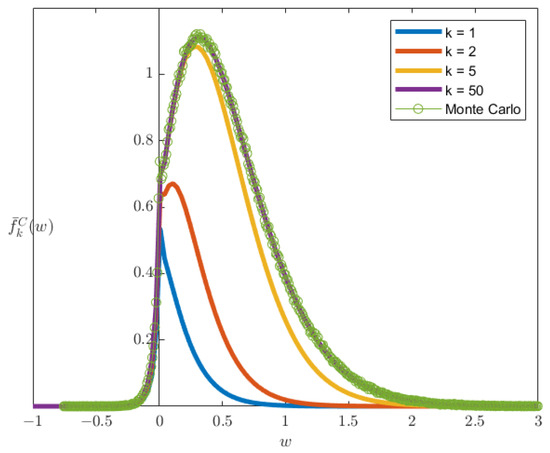
Figure 4.
Comparison of the truncated PDF from the Cui et al. (2016) approach with Monte-Carlo simulation results for , , , , and . Truncation levels () show improved estimation as k increases, with Monte-Carlo results (green circles) serving as the benchmark.
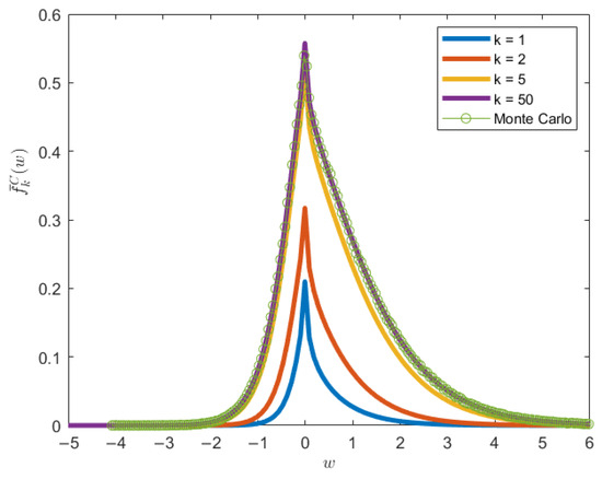
Figure 5.
Plot of the truncated PDF from the Cui et al. (2016) approach for , , , , and . Results are shown for truncation levels , with Monte-Carlo simulation (green circles) as the benchmark. The figure demonstrates improved estimation as k increases.
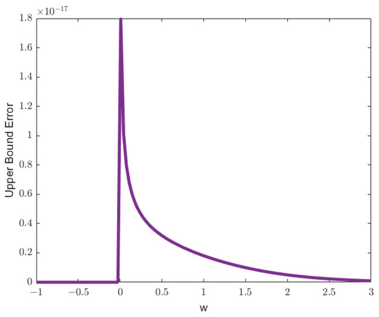
Figure 6.
Plot of the upper bound error function for , , , , , and truncation level . The function illustrates the maximum deviation introduced by the truncation for the specified parameters.
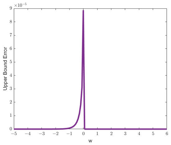
Figure 7.
Plot of the upper bound error function for , , , , , and truncation level . The plot demonstrates the maximum error introduced by the truncation for the given parameters, with the peak indicating regions of higher error magnitude.
The estimated PDF and CDF, as given in (10) and (12), using the trapezoidal rule of integration, show an excellent estimation. Figure 8 and Figure 9 show that the plot of the estimated PDF overlaps with the Monte-Carlo simulation, and Figure 10 and Figure 11 show that the estimated CDF is a reasonable estimation as it approaches 1 when , along with the increase in the number of divisions for the numerical integration. The upper bound error of the estimated PDF is also proportional to the number of divisions since the value of remains constant. Hence, the upper bound error for is the same plot for with the multiplication of to the upper bound value shown in Figure 12 and Figure 13.
Figure 8.
Plot of the PDF for , , , , , and .

Figure 9.
Plot of the PDF for , , , , , and .
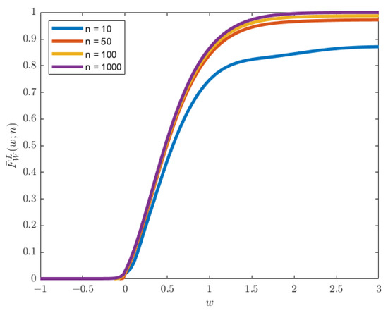
Figure 10.
Plot of the CDF for , , , , , and .
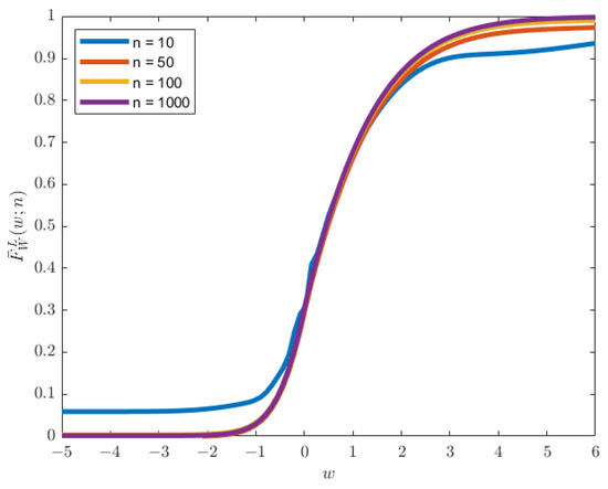
Figure 11.
Plot of the CDF for , , , , , and .
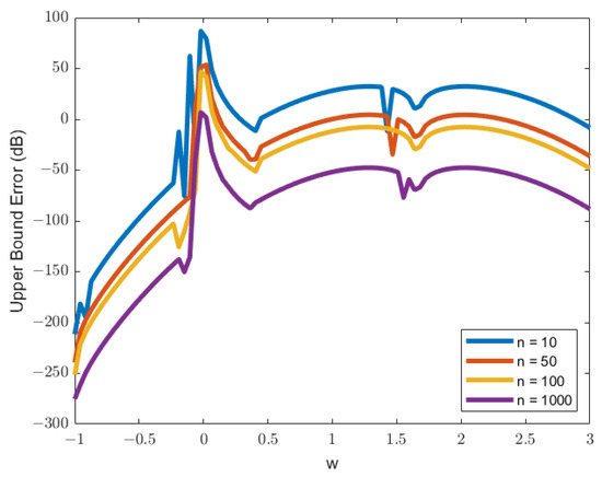
Figure 12.
Plot of the upper bound error function in dB for , , , , , and .
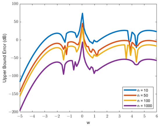
Figure 13.
Plot of the upper bound error function in dB for , , , , , and .
The upper bound errors shown in Figure 12 and Figure 13 have high errors not only near the peak of the PDF value but also at the end of the plot. The high errors can be the result of a change in the sign of the concavity of the plot. The small division value, , shows that the second derivative changes sign from positive to negative at the end of the plots.
In all cases of different correlation values, the proposition and the error-bound formula of the upper bound error function yield a considerably small value, indicating that the estimated PDFs provide a reasonable approximation of the exact distribution, as shown in Table 1. For some parameters, performs better than based on the upper bound error value.

Table 1.
Values of mean, median, and percentile of upper bound error of estimated PDF using the truncated PDF of [20] with and the numerical integral calculation of [42] using trapezoidal rule with .
The truncated PDF, , has many advantages. In Table 2, it is also shown that the truncated PDF in [20] requires less calculation than the numerical calculation of the PDF in [42] with the same upper bound error. The truncated PDF also required less computation time. The numerical calculation of the PDF using the trapezoidal rule requires a longer computation time due to the optimization algorithm. The result of the numerical calculation integral is also exposed because optimization can give a local minimum. The results in Table 2 are computed using Algorithms 2 and 3, respectively.
Table 2.
Values using the truncated PDF of [20] and using the numerical integral calculation of [42] using the trapezoidal rule given the predetermined .
However, has a disadvantage. For a large value of , the modified Bessel function of the second kind has computational limitations and can result in a zero value. In MATLAB, when . Hence, for the specified parameters that the software is able to compute, the truncated PDF in [20] gives a better upper bound error. For data with , the numerical calculation of PDF in [42] is preferred.
The numerical calculation PDF, , has many advantages. The estimated PDF does not require a Bessel function, which can have zero value in software computing when the domain is large. The calculation of the estimated PDF value uses only simple algebraic operations instead of a nested loop. The PDF in [42] is also written in a general form and not restricted to the product of two normal distributions. However, the upper bound error computation for requires an optimization algorithm and thus takes more time to calculate compared to the truncated PDF, .
In the following section, parameters from the application in conventional mass measurement are used. The parameters cause zero values for the estimated PDF of . The zero values are caused by the built-in function of besselk() in MATLAB, which produces zero values because of computational limitations. Therefore, only the estimated PDF of and the normal approximation of [35] can be used.
5. Application in Conventional Mass Measurement
The function of the random variables of the mass measurement in [13] consists of the summation and product. The function of random variables simplifies a more complex function in [51]. The simplification is due to eliminating the buoyancy effect on the weighing. The buoyancy correction function is not included, since the density of reference and the test weight density are rarely measured. However, the random variable function adds a sensitivity coefficient not found in [51]. The conventional mass measurement function is given by [13]
with
where
: conventional mass of reference weight;
S: balance sensitivity;
: conventional mass of sensitivity weight;
: indication balance of sensitivity weight;
: difference indication of test weight and reference weight.
In current practice, the random variable function of measurement is assumed to have a normal distribution based on [52]. This assumption disregards the complexity of the random variable function and treats all functions the same. While the normal approximation is not suited for some random variable functions, the approximation is satisfactory for some functions with specific parameter values. The normal approximation must be validated by Monte-Carlo simulation based on [53]. For complex random variable functions, the guidelines in [52,53] provide a few options. However, for the product of two random variables, more options are available.
The function of random variables in Equation (42) is a summation of two random variables, with one random variable being a product of two random variables. The primary focus is the estimated PDF and its upper bound error of the product of two random variables, S and . The value for the parameters of the random variables is taken from the sample statistics of actual data.
The data were collected at the Mass Laboratory, Ministry of Trade, West Java, Indonesia. The laboratory has a target temperature of 20 °C and humidity of 50%, with a tolerable discrepancy of ±2 °C and , respectively. The temperature is maintained by a ductless mini-split air conditioner with an air reflector to minimize the air current, and a dehumidifier maintains the humidity. The balance used is the model XP26C, with a readability of g and a maximum capacity of 20 g. The balance is equipped with hanging pan technology to eliminate eccentricity. It also has motorized inner draft shield doors to minimize the air current that can affect the weighing results. The weight that is used for sensitivity measurement is a wire type weight with a nominal mass of 500 mg class E2. It has a conventional mass of 500.0204 mg, with an uncertainty measurement of 0.0032 mg.
The sensitivity measurement is conducted using fifty weighings to produce fifty data points. The indication balance of the sensitivity weight is measured by subtracting the indication of the sensitivity weight from the zero reading indication. For the difference in the indication of the test weight and the reference weight, one hundred weighings were conducted to produce fifty data points. The weighing was conducted alternately with the reference weight and the test weight. The alternate weighing between the reference and test weights is known as ABBA weighing, where A and B represent the reference and test weights, respectively.
The empirical data of sensitivity have a mean of 1.00003, a standard deviation of , a kurtosis of 3.50435, and a skewness of . The empirical data on the difference between the indication of reference weight and test weight have a mean of mg, a standard deviation of mg, a kurtosis of 6.53806, and a skewness of 1.34834. The computed correlation between the sensitivity and the difference of indication is . The empirical data of the sensitivity is unitless, since they are the division of the mass and the balance of indication, which have the same unit. The difference between the reference weight and the test weight has a unit of mg. Even though the balance has a readability of 1 μg, the indication is in mg.
The empirical CDF and the CDF of the normal distribution for sensitivity are shown in Figure 14, and the difference in the indication weighing is shown in Figure 15. Each data point is tested with the Kolmogorov–Smirnov test for normality. For sensitivity data, the acceptance of the null hypothesis is , and for the difference of the reference and test weight data, the acceptance of the null hypothesis is .
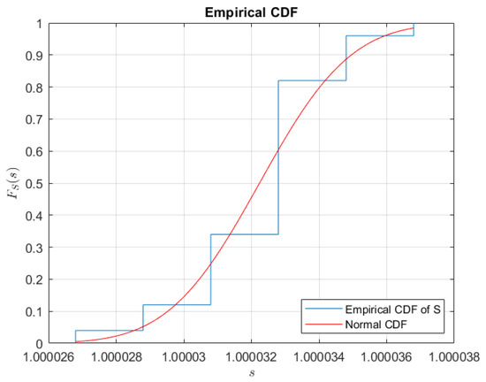
Figure 14.
Plot of the empirical CDF of the sensitivity coefficient, S, of balance.
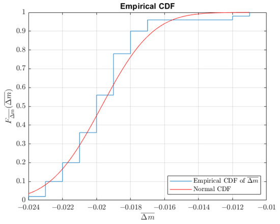
Figure 15.
Plot of the empirical CDF of the results difference between the standard and test weight, .
The empirical data on the product between sensitivity and difference have a mean of , a standard deviation of , a kurtosis of 6.53808, and a skewness of 1.34833. The estimated PDF and empirical CDF are shown in Figure 16 and Figure 17, respectively. The result shows that the random variable can be estimated by a normal distribution. This result follows [35], since ; even with , the result is still considered a normal distribution with based on the Kolmogorov–Smirnov test. The random variable of the product, W, can be considered a normal distribution, and has a normal distribution based on the certificate. Hence, the conventional mass measurement can be characterized by a normal distribution. This result supports the normal approximation of the measurement results based on [51].
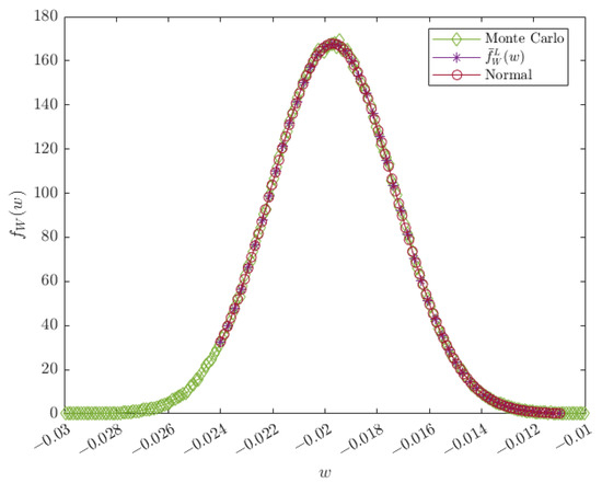
Figure 16.
Plot of the PDF product between the sensitivity and difference between the standard and test weight, .
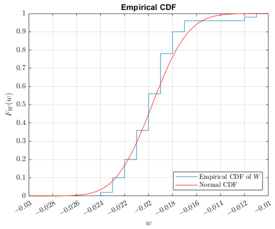
Figure 17.
Plot of the empirical CDF of the product between the sensitivity and difference between the standard and test weight, .
The upper bound error of is shown in Figure 18. The result shows that the error peaks near the mean and reduces as it approaches the mean value. The error shows an almost symmetrical plot; the slight asymmetry might be the cause of the skewness not being equal to zero. Based on Algorithm 3, the error for is less than , which can be considered sufficiently small compared to the PDF value, although for some parameters, the estimated PDF, , has a larger upper bound value compared to the truncated PDF, . For the specific conventional mass value, only the estimated PDF, , can be used. The truncated PDF, , does not give a result, since . In MATLAB, the besselk() function gives a zero value for the specified conventional mass measurement. The Algorithm 2 that uses Proposition 1 also aligns with the truncated PDF. The algorithm does not give k minimum, since is too large a value, giving an undefined value.
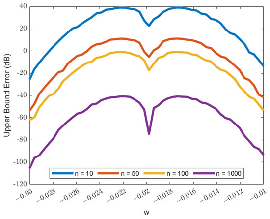
Figure 18.
Plot of the upper bound error in dB of the product of sensitivity, S, and the difference between the standard and test weight, .
6. Discussion
The proposition presented in this paper provides an upper bound for the truncation error in the PDF, which depends on the number of summation terms. This allows the error to be managed according to specified accuracy requirements by selecting an appropriate truncation level. However, the proposition is applicable only when the number of summations is sufficiently large to meet the given criteria. Numerical evaluations using the proposition and predetermined parameters indicate that the truncated PDF in [20] achieves an excellent estimation, with the maximum observed error not exceeding . However, the truncated PDF can not be used for some parameters, including those used in conventional mass measurement.
It is important to note that the proposition provides an upper bound rather than the exact truncation error. In practice, the actual error may be significantly smaller than the estimated bound. Further research could focus on deriving a tighter upper bound that more accurately reflects the truncation error. Additionally, future studies could extend this approach beyond the truncated PDF in [20] to other estimations, such as those proposed in [34], potentially improving the error estimation in broader contexts.
The CDF and the PDF given in [42] are the product of arbitrary distributions. Hence, they are not limited to the product of two normal random variables. They can also be used for the products of two unknown distributions. The unknown distribution is the result of a random variable function, where the CDF or PDF can be determined but not the distribution. One example is the product of two normal random variables. The PDF can be determined analytically, but the distribution is still unknown.
The estimated PDF in [42] is calculated using the numeric integral of the trapezoidal rule, which also gives excellent results, as shown in Table 1. By Table 2, the minimum number of divisions, , is still reasonable when the upper bound error is predetermined as . For future research, the numeric integral can be calculated using different methods with higher accuracy, such as Simpson’s rule. The upper bound error formula is also a well-known formula. The formula, however, requires the maximum value of the fourth derivative, which is more complex than the trapezoidal rule, which requires only the second derivative.
Author Contributions
Conceptualization, K.S. and R.S.; methodology, R.N.; software, R.N. and G.; validation, G., R.S., and K.S.; formal analysis, R.N.; resources, G.; data curation, R.N. and G.; writing—original draft preparation, R.N.; writing—review and editing, K.S.; funding acquisition, R.N. All authors have read and agreed to the published version of the manuscript.
Funding
This research was funded by the Indonesian Ministry of Trade for the financial support of the doctoral work of Rifyan Nasution.
Data Availability Statement
The datasets presented in this article are not readily available, because the data are intended for internal institutional use only. Requests to access the datasets should be directed to the corresponding author.
Acknowledgments
The authors would like to thank the editor and reviewers for their constructive comments, which led to improvements in the presentation of the manuscript. The first author would like to thank Aniq Atiqi Rohmawati for the valuable suggestions.
Conflicts of Interest
The authors declare no conflicts of interest.
References
- Kirkup, L.; Frenkel, R.B. An Introduction to Uncertainty in Measurement: Using the GUM (Guide to the Expression of Uncertainty in Measurement); Cambridge University Press: Cambridge, UK, 2006; ISBN 978-05-2160-579-3. [Google Scholar]
- Zhong, H.; Zhao, W.; Zhang, Z.; Wang, C.; Gao, K.; Wu, J. Investigation of discharge valve in ultra-high-speed rotary compressors: An experimental and FSI simulation-based study. Int. J. Refrig. 2024, 168, 730–741. [Google Scholar] [CrossRef]
- Abdel-Aziz, M.H.; Zoromba, M.S.; Attar, A.; Bassyouni, M.; Almutlaq, N.; Al-Qabandi, O.A.; Elhenawy, Y. Optimizing concentrated photovoltaic module efficiency using nanofluid-based cooling. Energy Convers. Manag. X 2025, 26, 100928. [Google Scholar] [CrossRef]
- Abu-Zeid, M.A.R.; Elhenawy, Y.; Toderaș, M.; Bassyouni, M.; Majozi, T.; Al-Qabandi, O.A.; Kishk, S.S. Performance enhancement of solar still unit using V-Corrugated basin, internal reflecting mirror, flat-plate solar collector and nanofluids. Sustainability 2024, 16, 655. [Google Scholar] [CrossRef]
- Altunay, F.M.; Pazarlıoğlu, H.K.; Guerdal, M.; Tekir, M.; Arslan, K.; Gedik, E. Thermal performance of Fe3O4/water nanofluid flow in a newly designed dimpled tube under the influence of non-uniform magnetic field. Int. J. Therm. Sci. 2022, 179, 107651. [Google Scholar] [CrossRef]
- Sousa, J.A.; Batista, E.; Demeyer, S.; Fischer, N.; Pellegrino, O.; Ribeiro, A.S.; Martins, L.L. Uncertainty calculation methodologies in microflow measurements: Comparison of GUM, GUM-S1 and Bayesian approach. Measurement 2021, 181, 109589. [Google Scholar] [CrossRef]
- Kim, J.H.; Lee, H.Y.; Lee, J.H. A study on metrological cross-validation of hydrogen refueling stations using a hybrid metrology evaluation system. Energy Rep. 2024, 11, 846–858. [Google Scholar] [CrossRef]
- Gürdal, M.; Pazarlıoğlu, H.K.; Tekir, M.; Altunay, F.M.; Arslan, K.; Gedik, E. Implementation of hybrid nanofluid flowing in dimpled tube subjected to magnetic field. Int. Commun. Heat Mass Transf. 2022, 134, 106032. [Google Scholar] [CrossRef]
- Somkun, S.; Sato, T.; Chunkag, V.; Pannawan, A.; Nunocha, P.; Suriwong, T. Performance comparison of ferrite and nanocrystalline cores for medium-frequency transformer of dual active bridge DC-DC converter. Energies 2021, 14, 2407. [Google Scholar] [CrossRef]
- Gaunt, R.E.; Nadarajah, S.; Pogány, T.K. Infinite divisibility of the product of two correlated normal random variables and exact distribution of the sample mean. J. Math. Anal. Appl. 2025, 552, 129800. [Google Scholar] [CrossRef]
- Eltawil, M.A.; Mohammed, M.; Alqahtani, N.M. Developing machine learning-based intelligent control system for performance optimization of solar PV-powered refrigerators. Sustainability 2023, 15, 6911. [Google Scholar] [CrossRef]
- Razumić, A.; Runje, B.; Alar, V.; Štrbac, B.; Trzun, Z. A review of methods for assessing the quality of measurement systems and results. Appl. Sci. 2025, 15, 9393. [Google Scholar] [CrossRef]
- Morris, E.C.; Fen, M.K. The Calibration of Weights and Balances; Monograph 4, NMI Technology Transfer Series; Australian Government, Department of Industry, Innovation and Science: Canberra, Australia, 2010.
- Ališić, Š.; Malengo, A.; Zelenka, Z.; Zůda, J.; Popa, G.; Mangutova-Stoilkovska, B.; Petkov, T. Pilot study comparison of developed and improved mass scale measurement capabilities. Meas. Sensors 2025, 38, 101354. [Google Scholar] [CrossRef]
- Su, Y.; Cheng, L.; Xiong, Z. Research regarding the double-weighing in air volume determination method. Meas. Sensors 2025, 38, 101357. [Google Scholar] [CrossRef]
- Meškuotienė, A.; Kaškonas, P.; Urbonavičius, B.G.; Dobilienė, J.; Raudienė, E. Ensuring measurement integrity in petroleum logistics: Applying standardized methods, protocols, and corrections. Appl. Sci. 2025, 15, 6886. [Google Scholar] [CrossRef]
- Cacais, F.; Delgado, J.U.; Loayza, V.; Rangel, J. In situ validation methodology for weighing methods used in preparing of standardized sources for radionuclide metrology. Metrology 2022, 2, 446–478. [Google Scholar] [CrossRef]
- Zelenka, Z.; Kolozinska, I. Stabilisation time after cleaning sheet and OIML shape weights. Meas. Sens. 2025, 38, 101359. [Google Scholar] [CrossRef]
- EURAMET Calibration Guide No. 19: Guidelines on the Determination of Uncertainty in Gravimetric Volume Calibration; EURAME: Braunschweig, Germany, 2018; Available online: https://www.euramet.org/Media/docs/Publications/calguides/I-CAL-GUI-019_Calibration_Guide_No._19_web.pdf (accessed on 2 April 2025).
- Cui, G.; Yu, X.; Iommelli, S.; Kong, L. Exact distribution for the product of two correlated Gaussian random variables. IEEE Signal Process. Lett. 2016, 23, 1662–1666. [Google Scholar] [CrossRef]
- Tabassum, H.; Hossain, E. On the deployment of energy sources in wireless-powered cellular networks. IEEE Trans. Commun. 2015, 63, 3391–3404. [Google Scholar] [CrossRef]
- Chizhik, D.; Foschini, G.J.; Gans, M.J.; Valenzuela, R.A. Keyholes, correlations, and capacities of multielement transmit and receive antennas. IEEE Trans. Wirel. Commun. 2002, 1, 361–368. [Google Scholar] [CrossRef]
- Gesbert, D.; Bolcskei, H.; Gore, D.A.; Paulraj, A.J. Outdoor MIMO wireless channels: Models and performance prediction. IEEE Trans. Commun. 2002, 50, 1926–1934. [Google Scholar] [CrossRef]
- Moura, J.M.; Jin, Y. Detection by time reversal: Single antenna. IEEE Trans. Signal Process. 2006, 55, 187–201. [Google Scholar] [CrossRef]
- Jin, Y.; Moura, J.M. Time-reversal detection using antenna arrays. IEEE Trans. Signal Process. 2008, 57, 1396–1414. [Google Scholar] [CrossRef]
- Colone, F.; Lombardo, P. Noncoherent adaptive detection in passive radar exploiting polarimetric and frequency diversity. IET Radar Sonar Navig. 2016, 10, 15–23. [Google Scholar] [CrossRef]
- Lopez-Morales, M.J.; Chen-Hu, K.; Garcia-Armada, A. Differential data-Aided channel estimation for up-link massive SIMO-OFDM. IEEE Open J. Commun. Soc. 2020, 1, 976–989. [Google Scholar] [CrossRef]
- Li, Y.; He, Q.; Blum, R.S. On the product of two correlated complex gaussian random variables. IEEE Signal Process. Lett. 2019, 27, 16–20. [Google Scholar] [CrossRef]
- Bielak, Ł.; Grzesiek, A.; Janczura, J.; Wyłomańska, A. Market risk factors analysis for an international mining company: Multidimensional, heavy-tailed-based modelling. Resour. Policy 2021, 74, 102308. [Google Scholar] [CrossRef]
- Adamska, J.; Bielak, Ł.; Janczura, J.; Wyłomańska, A. From multi-to univariate: A product random variable with an application to electricity market transactions—Pareto and Student’s t-Distribution case. Mathematics 2022, 10, 3371. [Google Scholar] [CrossRef]
- Nasrin, S.F.; Rajivganthi, C. Dynamical analysis of a stochastic Ebola model with nonlinear incidence functions. J. Nonlinear Sci. 2025, 35, 33. [Google Scholar] [CrossRef]
- Gaunt, R.E. Stein’s Method and the distribution of the product of zero-mean correlated normal random variables. Commun. Stat. Theory Methods 2021, 50, 280–285. [Google Scholar] [CrossRef]
- Craig, C.C. On the frequency function of xy. Ann. Math. Stat. 1936, 7, 1–15. [Google Scholar] [CrossRef]
- Seijas-Macías, A.; Oliveira, A. An approach to distribution of the product of two normal variables. Discuss. Math. Probab. Stat. 2012, 32, 87–99. [Google Scholar] [CrossRef]
- Aroian, L.A. The probability function of the product of two normally distributed variables. Ann. Math. Stat. 1947, 18, 265–271. [Google Scholar] [CrossRef]
- Nadarajah, S.; Pogány, T.K. On the distribution of the product of correlated normal random variables. C. R. Math. 2016, 354, 201–204. [Google Scholar] [CrossRef]
- Gaunt, R.E. A Note on the distribution of the product of zero-mean correlated normal random variables. Stat. Neerl. 2019, 73, 176–179. [Google Scholar] [CrossRef]
- Gaunt, R.E. Absolute moments of the variance-gamma distribution. J. Math. Anal. Appl. 2025, 543, 128861. [Google Scholar] [CrossRef]
- Gaunt, R.E.; Ye, Z. Asymptotic approximations for the distribution of the product of correlated normal random variables. J. Math. Anal. Appl. 2025, 543, 128987. [Google Scholar] [CrossRef]
- Gradshteyn, I.S.; Ryzhik, I.M. Table of Integrals, Series, and Products, 7th ed.; Academic Press: San Diego, CA, USA, 2007. [Google Scholar]
- Simon, M.K. Probability Distributions Involving Gaussian Random Variables: A Handbook for Engineers and Scientists; Kluwer Academic Publishers: Boston, MA, USA; Dordrecht, The Netherlands; London, UK, 2002; ISBN 978-0387346571. [Google Scholar]
- Ly, S.; Pho, K.H.; Ly, S.; Wong, W.K. Determining distribution for the product of random variables by using copulas. Risks 2019, 7, 23. [Google Scholar] [CrossRef]
- Rohatgi, V.K. An Introduction to Probability Theory Mathematical Studies; Wiley: New York, NY, USA, 1976. [Google Scholar]
- Segura, J. Bounds for ratios of modified Bessel functions and associated Turán-type inequalities. J. Math. Anal. Appl. 2011, 374, 516–528. [Google Scholar] [CrossRef]
- Watson, G.N. A Treatise on the Theory of Bessel Functions; The University Press: Cambridge, UK, 1922; Volume 3. [Google Scholar]
- Ly, S.; Pho, K.H.; Ly, S.; Wong, W.K. Determining distribution for the quotients of dependent and independent random variables by using copulas. J. Risk Financ. Manag. 2019, 12, 42. [Google Scholar] [CrossRef]
- Meyer, C. The Bivariate normal copula. Commun. Stat. Theory Methods 2013, 42, 2402–2422. [Google Scholar] [CrossRef]
- Bhatnagar, G.; Rajkumar, K. Telescoping continued fractions for the error term in Stirling’s formula. J. Approx. Theory 2023, 293, 105943. [Google Scholar] [CrossRef]
- Robbins, H. A Remark on Stirling’s formula. Am. Math. Mon. 1955, 62, 26–29. [Google Scholar] [CrossRef]
- Seijas-Macías, A.; Oliveira, A.; Oliveira, T.A.; Leiva, V. Approximating the distribution of the product of two normally distributed random variables. Symmetry 2020, 8, 1201. [Google Scholar] [CrossRef]
- International Organization of Legal Metrology (OIML). OIML R 111: Weights of Classes E1, E2, F1, F2, M1, M2, M3; OIML: Paris, France, 2004; Available online: https://www.oiml.org/en/files/pdf_r/r111-1-e04.pdf (accessed on 2 May 2025).
- International Organization for Standardization; International Electrotechnical Commission; International Bureau of Weights and Measures; International Organization of Legal Metrology. Evaluation of Measurement Data—Guide to the Expression of Uncertainty in Measurement; JCGM 100:2008; BIPM: Sèvres, France, 2008; Available online: https://www.bipm.org/documents/20126/2071204/JCGM_100_2008_E.pdf (accessed on 2 May 2025).
- International Bureau of Weights and Measures (BIPM); International Organization for Standardization (ISO); International Electrotechnical Commission (IEC); International Organization of Legal Metrology (OIML). Evaluation of Measurement Aata—Supplement 1 to the “Guide to the Expression of Uncertainty in Measurement”—Propagation of Distributions Using a Monte Carlo Method; JCGM 101:2008; BIPM: Sèvres, France, 2008; Available online: https://www.bipm.org/documents/20126/2071204/JCGM_101_2008_E.pdf/325dcaad-c15a-407c-1105-8b7f322d651c (accessed on 2 May 2025).
Disclaimer/Publisher’s Note: The statements, opinions and data contained in all publications are solely those of the individual author(s) and contributor(s) and not of MDPI and/or the editor(s). MDPI and/or the editor(s) disclaim responsibility for any injury to people or property resulting from any ideas, methods, instructions or products referred to in the content. |
© 2025 by the authors. Licensee MDPI, Basel, Switzerland. This article is an open access article distributed under the terms and conditions of the Creative Commons Attribution (CC BY) license (https://creativecommons.org/licenses/by/4.0/).