Sinusoidal Approximation Theorem for Kolmogorov–Arnold Networks

Abstract

The Kolmogorov–Arnold representation theorem states that any continuous multivariable function can be exactly represented as a finite superposition of continuous single-variable functions. Subsequent simplifications of this representation involve expressing these functions as parameterized sums of a smaller number of unique monotonic functions. Kolmogorov–Arnold Networks (KANs) have been recently proposed as an alternative to multilayer perceptrons. KANs feature learnable nonlinear activations applied directly to input values, modeled as weighted sums of basis spline functions. This approach replaces the linear transformations and sigmoidal post-activations used in traditional perceptrons. In this work, we propose a novel KAN variant by replacing both the inner and outer functions in the Kolmogorov–Arnold representation with weighted sinusoidal functions of learnable frequencies. We particularly fix the phases of the sinusoidal activations to linearly spaced constant values and provide a proof of their theoretical validity. We also conduct numerical experiments to evaluate its performance on a range of multivariable functions, comparing it with fixed-frequency Fourier transform methods, basis spline KANs (B-SplineKANs), and multilayer perceptrons (MLPs). We show that it outperforms the fixed-frequency Fourier transform B-SplineKAN and achieves comparable performance to MLP.

1. Introduction

The quest to represent complex mathematical functions in terms of simpler constituent parts is a central theme in analysis and applied mathematics. A pivotal moment in this endeavor arose from the list of 23 problems presented by David Hilbert in 1900, which profoundly shaped the mathematical landscape of the 20th century. Hilbert’s 13th problem, in particular, posed a fundamental question about the limits of function composition. The problem seeks solutions to a general 7th-degree polynomial, which are finite combinations of functions of a single variable each, i.e., if $f(x_1,\dots x_7)=g(f_1\left(x_1\right),\dots f_7\left(x_7\right))$, where g is a simple known function. [1,2].

In the late 1950s, Andreĭ Kolmogorov and his graduate student Vladimir Arnold provided a powerful and affirmative answer to this problem. Their work culminated in the Kolmogorov–Arnold representation theorem (KART) [3,4], which states that any multivariable continuous function f defined on a compact domain, such as the n-dimensional unit cube, can be represented exactly by a finite superposition of single variable functions and the single binary operation of addition. The canonical form of the theorem is expressed as

$$f(x_1,\dots ,x_n)=\sum _{q=0}^{2n}{\varphi }_q\left(\sum _{p=1}^n{\psi }_{p,q}\left(x_p\right)\right),$$

(1)

where ${\psi }_{p,q}:\mathbb{R}\to \mathbb{R}$ are the innerfunctions, and ${\varphi }_q:\mathbb{R}\to \mathbb{R}$ are the outer functions, which are assumed to be continuous. Lorentz [5] and Sprecher [6] showed that the functions ${\varphi }_q$ can be replaced by only one function $\varphi$ and that the functions ${\psi }_{p,q}$ can be replaced by ${\lambda }^{pq}{\psi }_q$, where $\lambda$ is a constant and ${\psi }_q$ are monotonic and Lipschitz-continuous functions.

Perceptrons were introduced around the same time by Frank Rosenblatt [7] for simple classification tasks. However, their limitations were famously highlighted in the 1969 book “Perceptrons” by Marvin Minsky and Seymour Papert [8]. They proved that a single-layer perceptron could not solve problems that were not linearly separable, such as the simple XOR logical function. This critique led to a significant decline in neural network research for over a decade, often termed the first “AI winter.” The revival came in the 1980s with the popularization of the multilayer perceptron (MLP), which was introduced in the late 1960s [9]. By adding one or more “hidden” layers between the input and output layers, MLPs could overcome the limitations of the single-layer perceptron. The key breakthrough that made these deeper networks practical was the backpropagation algorithm. While developed earlier, its popularization by David Rumelhart, Geoffrey Hinton, and Ronald Williams in 1986 [10] provided an efficient method to train the weights in these new, multilayered networks, sparking a renewed wave of interest in the field.

With MLPs and derived neural network architectures demonstrating practical success [11,12,13], the next crucial step was to understand their theoretical capabilities. The Universal Approximation Theorem provides this foundation, showing that a standard MLP with just one hidden layer can, in principle, approximate any continuous function to any desired degree of accuracy. George Cybenko [14] used tools from functional analysis, like the Hahn–Banach theorem and the Riesz representation theorem, and showed that, given any multivariable continuous function in a compact domain, there exist values of the weights and biases of a multilayer perceptron with a sigmoidal model whose loss with respect to the function is bound by any given positive value $ϵ$. Almost concurrently, Kurt Hornik, Maxwell Stinchcombe, and Halbert White [15] provided a different, more general proof for the universal approximation property of a multilayer perceptron with any bounded, non-constant, and continuous activation function.

The applicability of KART to continuous functions in a compact domain was first highlighted by Hecht-Nielsen [16,17]. However, the functions constructed in Kolmogorov’s proofs, as well as in their later simplifications or improvements, are highly complex and non-smooth, which were very different from the much simpler activation functions used in MLPs [18]. Soon, a series of papers by Věra Kůrková [19,20] showed that the one-dimensional inner and outer functions could be approximated using two-layer MLPs and obtained a relationship between the number of hidden units and the loss based on the properties of the function being approximated.

It was not until much later in the 2020s that KART had a direct practical application in the domain of neural networks and machine learning. Kolmogorov–Arnold networks (KANs) were first proposed by Liu et al. [21,22] as an alternative to MLPs, which demonstrated interpretable hidden activations and higher regression accuracy. They used learnable basis splines to model the constituent hidden values, similar to KART, and their stacked representation is simplified compared to the original form used in KART. Subsequent works retained the same representation but replaced splines with other series of functions, such as radial basis functions and Chebyshev polynomials [23,24,25,26], which were computationally faster and demonstrated superior scaling properties with larger numbers of learnable parameters. However, issues of speed and numerical stability on smaller floating-point types remain, especially compared to the well-established MLPs [27,28].

To address these challenges, we propose a variant of the representation theorems by Lorentz [5] and Sprecher [6]. We set the phases of the sinusoidal activations to linearly spaced constant values and establish their mathematical foundation to confirm their validity. Previous work has explored this approximation series compared to MLPs and basis-spline approximations and showed competitive performance on the inherently discontinuous domain task of labeling hand-written numerical characters [29]. We extend this work by providing a constructive proof of the approximation series for single-variable and multivariable functions and evaluating performance on several such functions with features such as rapid and changing oscillation frequencies. We also extend the comparison from [29] to include fixed-frequency Fourier transform methods and MLP with piecewise-linear and periodic activation functions.

Table 1. Simplifications proposed for the Kolmogorov–Arnold representation theorem at different points in time.

Version	Representation
Kolmogorov (1957)	${\displaystyle \sum _{q=0}^{2d}{g}_q\left({\displaystyle \sum _{p=1}^d{\psi }_{pq}\left(x_p\right)}\right)}$
Lorentz–Sprecher (1965)	${\displaystyle \sum _{q=0}^{2d}}g\left({\displaystyle \sum _{p=1}^d{\lambda }_p\psi (x_p+qa)+c_q}\right)$
KAN, B-spline basis (2024)	$\begin{array}{cc}\hfill y_i& ={\displaystyle {\displaystyle {\displaystyle \sum _{j=1}^d}\sum _{k=1}^{G+p}{w}_{ijk}{B}_{k,p}\left(x_j\right)+b_i}}\hfill \\ \hfill \Rightarrow & {\displaystyle \sum _{i=1}^H\sum _{l=1}^{G+p}}{W}_{il}{B}_l\left(y_i\right)+\beta \hfill \end{array}$
KAN, sinusoidal basis (ours)	$\begin{array}{cc}\hfill y_q& =\sum _{p=1}^d\sum _{k=0}^N{A}_{pq,k}sin({\omega }_{1k}{x}_p+{\phi }_{1k})\hfill \\ \hfill \Rightarrow & \sum _{q=1}^{2d+1}\sum _{j=0}^N{B}_{qj}sin\left({\omega }_{2j}{y}_q+{\phi }_{2j}\right)\hfill \end{array}$

summarizes the advancements in this area.

The remainder of this paper is organized as follows. In Section 2, we establish the necessary auxiliary results to prove the approximation theorem for one-dimensional functions. Section 3 extends the results from the previous section to derive a universal approximation theorem for two-layer neural networks. In Section 4, we test several functions and compare the numerical performance of our proposed networks with the classical Fourier transform. Finally, in Section 5, we discuss potential applications and future research directions.

2. Sinusoidal Universal Approximation Theorem

The concept of approximating any function using simple, manageable functions has been widely utilized in deep learning and neural networks. In addition to the multilayer perceptron (MLP) approach, the Kolmogorov–Arnold representation theorem (KART) has gained increasing attention from data scientists, who have developed Kolmogorov–Arnold Networks (KANs) to create more interpretable neural networks. In the classical Fourier transform, any continuous, piecewise continuously differentiable ($C^1$) function on a compact interval can be expressed as a Fourier series of sine and cosine functions. In contrast, Kolmogorov demonstrated that any continuous multivariable function can be represented as form (1).

By extending Kolmogorov’s idea and refining both outer and inner functions using sine terms, we can demonstrate that any continuous function in $[0,1]$ can be approximated by a finite sum of sinusoidal functions with varying frequencies and linearly spaced phases.

Theorem 1.

Let f be a continuous function on $[0,1]$ and $0<\alpha \le {\displaystyle \frac{\pi }{2}}$. For any $ϵ>0$, there exist $N\in \mathbb{N}$, frequencies ${\omega }_k\in [0,2\pi ]$, and coefficients $A_k\in \mathbb{R}$ such that

$$\underset{0\le x\le 1}{sup}|f\left(x\right)-\sum _{k=0}^N{A}_{k}sin\left({\omega }_{k}x+{\displaystyle \frac{k\alpha }{N+1}})\right|<ϵ.$$

(2)

To prove this theorem, we need a series of lemmas to approximate the sine function with its Taylor series and then apply the Weierstrass approximation theorem to bring the sum of sinusoidal functions arbitrarily close to any continuous function.

First, we need to approximate the sinusoidal function using its Taylor polynomial.

Lemma 1.

Let $\omega \in [0,2\pi ]$ and $\alpha \in \mathbb{R}$. For every $N\in \mathbb{N}$,

$$\underset{0\le x\le 1}{sup}\left|sin(\omega x+\alpha )-T_N(\omega ,\alpha ,x)\right|\le {\displaystyle \frac{{\left(2\pi \right)}^{N+1}}{(N+1)!}},$$

where

$$T_N(\omega ,\alpha ,x)=\sum _{l=0}^N{\displaystyle \frac{{\omega }^l}{l!}}sin(\alpha +{\displaystyle \frac{l\pi }{2}})x^l.$$

(3)

Proof. 

Set $g\left(x\right)=sin(\omega x+\alpha )$. We can rewrite

$$g\left(x\right)=sin(\omega x+\alpha )=T_N(\omega ,\alpha ,x)+R_N\left(x\right),$$

where $T_N(\omega ,\alpha ,x)$, determined by (3), is the Taylor polynomial of the function $g\left(x\right)$ centered at $x=0$, and the remainder

$$R_N\left(x\right)={\displaystyle \frac{g^{(N+1)}\left(\xi \right)}{(N+1)!}}{x}^{N+1},$$

for some $\xi \in (0,1)$.

Since $\omega \in [0,2\pi ]$ and $\xi \in (0,1)$,

$$\left|g^{(N+1)}\left(\xi \right)\right|=|{\omega }^{N+1}sin\left(\omega \xi +(N+1)\pi /2\right)|\le {\omega }^{N+1}\le {\left(2\pi \right)}^{N+1}.$$

Therefore,

$$|sin(\omega x+\alpha )-T_N(\omega ,\alpha ,x)|=|R_N\left(x\right)|={\displaystyle \frac{|g^{(N+1)}\left(\xi \right)|}{(N+1)!}}{\left|x\right|}^{N+1}\le {\displaystyle \frac{{\left(2\pi \right)}^{N+1}}{(N+1)!}}$$

for all $x\in [0,1]$. This completes the proof of Lemma 1.    □

Lemma 2.

For every $ϵ>0$, there exists $N_0\in \mathbb{N}$ such that for all $N>N_0$,

$$\underset{0\le x\le 1}{sup}\left|\sum _{k=0}^N{A}_{k}sin({\omega }_{k}x+{\alpha }_k)-\sum _{k=0}^N{A}_k{T}_N({\omega }_k,{\alpha }_k,x)\right|<ϵ,$$

(4)

where ${\omega }_k\in [0,2\pi ]$, ${\alpha }_k,A_k\in \mathbb{R}$, and $T_N({\omega }_k,{\alpha }_k,x)$ is determined by (3).

Proof. 

From Lemma 1, we have

$$\underset{0\le x\le 1}{sup}\left|sin({\omega }_{k}x+{\alpha }_k)-T_N({\omega }_k,{\alpha }_k,x)\right|\le {\displaystyle \frac{{\left(2\pi \right)}^{N+1}}{(N+1)!}}$$

for ${\omega }_k\in [0,2\pi ]$, ${\alpha }_k\in \mathbb{R}$, $0\le k\le N$, and $N\in \mathbb{N}$. Therefore,

$$\begin{array}{cc}\hfill & \underset{0\le x\le 1}{sup}\left|\sum _{k=0}^N{A}_{k}sin({\omega }_{k}x+{\alpha }_k)-\sum _{k=0}^N{A}_k{T}_N({\omega }_k,{\alpha }_k,x)\right|\hfill \\ \hfill \le & \sum _{k=0}^N\left|A_k\right|\underset{0\le x\le 1}{sup}|sin({\omega }_{k}x+{\alpha }_k)-T_N({\omega }_k,{\alpha }_k,x)|\hfill \\ \hfill \le & \sum _{k=0}^N{\displaystyle \frac{{\left(2\pi \right)}^{N+1}\left|A_k\right|}{(N+1)!}}\le {\displaystyle \frac{{\left(2\pi \right)}^{N+1}}{N!}}\underset{k}{max}\left|A_k\right|.\hfill \end{array}$$

Since $\underset{N\to \infty }{lim}{\displaystyle \frac{{\left(2\pi \right)}^{N+1}}{N!}}=0$, for a given $ϵ>0$, we can choose $N_0\in \mathbb{N}$ such that for all $N>N_0$, we obtain (4) to complete the proof of Lemma 3.   □

Lemma 3

(Weierstrass Approximation [30]). Let f be a continuous function on $[0,1]$. Then, for any $ϵ>0$, there exists $N_0$ such that for all $N>N_0$

$$\underset{0\le x\le 1}{sup}\left|f\left(x\right)-B_N(f,x)\right|<ϵ,$$

where $B_N(f,x)$ is the Bernstein polynomial of f determined by

$$B_N(f,x)=\sum _{l=0}^{N}f\left({\displaystyle \frac{l}{N}}\right)\left({\displaystyle \genfrac{}{}{0pt}{}{N}{l}}\right)x^l{(1-x)}^{N-l}.$$

(5)

Lemma 4.

Let $p\left(x\right)={\displaystyle \sum _{l=0}^N}{b}_l{x}^l$ be any polynomial, and let $0<{\alpha }_k<{\displaystyle \frac{\pi }{2}}$ for all $0\le k\le N$. Then, there exists ${\omega }_k\in [0,2\pi ]$ and $A_k\in \mathbb{R}$ such that

$$p\left(x\right)=\sum _{k=0}^N{A}_k{T}_N({\omega }_k,{\alpha }_k,x)$$

(6)

for all $x\in [0,1]$, where $T_N({\omega }_k,{\alpha }_k,x)$ is determined by (3).

Proof. 

Recall the formula determined by (3); then, we have

$$\begin{array}{cc}\hfill \sum _{k=0}^N{A}_k{T}_N({\omega }_k,{\alpha }_k,x)=& \sum _{k=0}^N\sum _{l=0}^N{A}_k{\displaystyle \frac{{\omega }_k^{l}sin({\alpha }_k+\frac{l\pi }{2})x^l}{l!}}\hfill \\ \hfill =& \sum _{l=0}^N\left(\sum _{k=0}^N{\displaystyle \frac{A_k{\omega }_k^{l}sin({\alpha }_k+\frac{l\pi }{2})}{l!}}\right)x^l.\hfill \end{array}$$

To obtain (6), we need to choose ${\omega }_k$ and $A_k$ such that

$$\sum _{k=0}^N{\displaystyle \frac{A_k{\omega }_k^{l}sin({\alpha }_k+\frac{l\pi }{2})}{l!}}=b_l,0\le l\le N.$$

Equivalently, we need to find ${\omega }_k$ and $A_k$ such that

$$\sum _{k=0}^N{A}_k{\omega }_k^{l}sin({\alpha }_k+{\displaystyle \frac{l\pi }{2}})=b_l·l!,0\le l\le N.$$

(7)

Consider the following $(N+1)\times (N+1)$ matrix:

$$M=\left[\begin{array}{cccc}sin\left({\alpha }_0\right)& sin\left({\alpha }_1\right)& \cdots & sin\left({\alpha }_N\right)\\ {\omega }_{0}sin({\alpha }_0+{\displaystyle \frac{\pi }{2}})& {\omega }_{1}sin({\alpha }_1+{\displaystyle \frac{\pi }{2}})& \cdots & {\omega }_{N}sin({\alpha }_N+{\displaystyle \frac{\pi }{2}})\\ ⋮& \ddots & \cdots & ⋮\\ {\omega }_0^{N}sin({\alpha }_0+{\displaystyle \frac{N\pi }{2}})& {\omega }_1^{N}sin({\alpha }_1+{\displaystyle \frac{N\pi }{2}})& \cdots & {\omega }_N^{N}sin({\alpha }_N+{\displaystyle \frac{N\pi }{2}})\end{array}\right].$$

Since $0<{\alpha }_k<{\displaystyle \frac{\pi }{2}}$, $sin({\alpha }_k+{\displaystyle \frac{l\pi }{2}})\ne 0$ for all $0\le l\le N$. By induction in N, we can select ${\omega }_0,{\omega }_1,\dots ,{\omega }_N\in [0;2\pi ]$ such that $det\left(M\right)\ne 0$. Therefore, the system of Equation (7) with the augmented matrix M has a solution for $A_0,A_1,\dots ,A_N$. This completes the proof of Lemma 4.    □

Proof of Theorem 1. 

For a given $ϵ>0$, according to Lemmas 2 and 3, there exists $N_0\in \mathbb{N}$ such that for all $N>N_0$, we have

$$\underset{0\le x\le 1}{sup}\left|f\left(x\right)-p\left(x\right)\right|<ϵ/2,$$

(8)

where $p\left(x\right)=B_N(f,x)$ is the Bernstein polynomial of f, and

$$\underset{0\le x\le 1}{sup}\left|\sum _{k=0}^N{A}_{k}sin({\omega }_{k}x+{\alpha }_k)-\sum _{k=0}^N{A}_k{T}_N({\omega }_k,{\alpha }_k,x)\right|<ϵ/2$$

(9)

for some ${\omega }_k,A_k$ (to be chosen later) and ${\alpha }_k={\displaystyle \frac{k\alpha }{N+1}}\in (0,{\displaystyle \frac{\pi }{2}})$.

By virtue of Lemma 4, we can find ${\omega }_k\in [0,2\pi ]$ and $A_k\in \mathbb{R}$ such that

$$p\left(x\right)=\sum _{k=0}^N{A}_k{T}_N({\omega }_k,{\alpha }_k,x).$$

Now, combining (8) and (9), we obtain the conclusion of Theorem 1.   □

3. Sinusoidal Approximation Theorem for Two-Layer Neural Networks

We next extend the result of Theorem 1 to approximate any continuous function defined on a compact domain in ${\mathbb{R}}^n$. To simplify the treatment of function extension, we restrict our attention to functions supported within the unit cube $I^n={[0,1]}^n$. Under this setting, a two-layer neural network with sinusoidal activation functions can approximate any continuous function on the unit cube. A similar result for sigmoidal activation functions was established by Kůrková in [20]. The main goal of this section is to approximate a continuous function on a compact domain by a finite sum of nested sinusoidal functions of the form

$$\sum _{j=0}^M{B}_{j}sin({\nu }_j\sum _{p=1}^n\sum _{k=0}^N{A}_{pk}^{j}sin({\omega }_k{x}_p+{\phi }_k)+{\gamma }_j),$$

(10)

where $B_j,A_{pk}^j\in \mathbb{R}$ are coefficients, ${\nu }_j,{\omega }_k\in [0,2\pi ]$ are frequencies, and ${\phi }_k,{\gamma }_j\in (0,{\displaystyle \frac{\pi }{2}}]$ are phases.

Theorem 2.

Let $f:I^n\to \mathbb{R}$ be a continuous function. For any $\epsilon >0$, there exists $M,N\in \mathbb{N}$, $A_{pq,k},B_{qj}\in \mathbb{R}$, ${\omega }_{1k},{\omega }_{2j}\in [0,2\pi ]$, and ${\phi }_{1k},{\phi }_{2j}\in (0,{\displaystyle \frac{\pi }{2}}]$ such that

$$|f(x_1,\dots ,x_n)-\sum _{q=1}^{2n+1}\sum _{j=0}^M{B}_{qj}sin({\omega }_{2j}\sum _{p=1}^n\sum _{k=0}^N{A}_{pq,k}sin({\omega }_{1k}{x}_p+{\phi }_{1k})+{\phi }_{2j})|<\epsilon .$$

(11)

Proof. 

According to the Kolmogorov Theorem, any continuous function $f:I^n\to \mathbb{R}$ can be written as

$$f(x_1,\dots ,x_n)=\sum _{q=1}^{2n+1}{\varphi }_q\left(\sum _{p=1}^n{\psi }_{pq}\left(x_p\right)\right),$$

where ${\varphi }_q$ and ${\psi }_{pq}$ are continuous functions on the number line.

Each function ${\psi }_{pq}$ is continuous, and the sum ${\sum }_{p=1}^n{\psi }_{pq}\left(x_p\right)$ is bounded for all $x\in I^n$. This means that

$$a\le \sum _{p=1}^n{\psi }_{pq}\left(x_p\right)\le b$$

for some $a,b\in \mathbb{R}$ and for all $(x_1,\dots ,x_n)\in I^n$.

Now, the function ${\varphi }_q$ is uniformly continuous on $[a,b]$, so for the given $\epsilon$, there exists ${\delta }_1>0$ such that

$$|{\varphi }_q\left(u\right)-{\varphi }_q\left(v\right)|<\epsilon /(4n+2)$$

(12)

whenever $|u-v|<{\delta }_1$.

For each function ${\psi }_{pq}\left(x_p\right)$, according to Theorem 1, there exists $A_{pq,k},w_{1k}$ and ${\phi }_{1k}$ such that

$$|{\psi }_{pq}\left(x_p\right)-\sum _{k=0}^N{A}_{pq,k}sin(w_{1k}{x}_p+{\phi }_{1k})\mid <{\delta }_1/n.$$

Therefore,

$$\begin{array}{cc}& |\sum _{p=1}^n{\psi }_{pq}\left(x_p\right)-\sum _{p=1}^n(\sum _{k=0}^N{A}_{pq,k}sin(w_{1k}{x}_p+{\phi }_{1k})\left)\right|\hfill \\ \hfill \le & \sum _{p=1}^n|{\psi }_{pq}\left(x_p\right)-(\sum _{k=0}^N{A}_{pq,k}sin(w_{1k}{x}_p+{\phi }_{1k})\left)\right|\hfill \\ \hfill <& \sum _{p=1}^n{\delta }_1/n={\delta }_1.\hfill \end{array}$$

Now, we apply (12) to $u={\displaystyle \sum _{p=1}^n}{\psi }_{pq}\left(x_p\right)$ and $v={\displaystyle \sum _{p=1}^n}({\displaystyle \sum _{k=0}^N}{A}_{pq,k}sin(w_{1k}{x}_p+{\phi }_{1k}))$ to obtain

$$|{\varphi }_q(\sum _{p=1}^n{\psi }_{pq}\left(x_p\right))-{\varphi }_q(\sum _{p=1}^n(\sum _{k=0}^N{A}_{pq,k}sin(w_{1k}{x}_p+{\phi }_{1k}))\left)\right|<\epsilon /(4n+2).$$

(13)

By applying Theorem 1 to ${\varphi }_q$, we obtain the coefficients $B_{qj}$, frequencies $w_{2j}$, and phases ${\phi }_{2j}$ such that

$$|{\varphi }_q(\sum _{p=1}^n\sum _{k=0}^N{A}_{pq,k}sin(w_{1k}{x}_p+{\phi }_{1k}))-\sum _{j=0}^M{B}_{qj}sin(w_{2j}(\sum _{p=1}^n(\sum _{k=0}^N{A}_{pq,k}sin(w_{1k}{x}_p+{\phi }_{1k})))+{\phi }_{2j})|<{\delta }_2$$

(14)

where ${\delta }_2=\epsilon /(4n+2)$.

Combining (13) and (14) yields

$$|{\varphi }_q(\sum _{p=1}^n{\psi }_{pq}(x_p))-\sum _{j=0}^M{B}_{qj}sin(w_{2j}\left(\sum _{p=1}^n\right(\sum _{k=0}^N{A}_{pq,k}sin(w_{1k}{x}_p+{\phi }_{1k})\left)\right)+{\phi }_{2j}\left)\right|<\epsilon /(2n+1).$$

The last inequality follows that

$$\begin{array}{cc}& |f(x_1,\dots ,x_n)-\sum _{q=1}^{2n+1}\sum _{j=0}^M{B}_{qj}sin(w_{2j}\left(\sum _{p=1}^n\right(\sum _{k=0}^N{A}_{pq,k}sin(w_{1k}{x}_p+{\phi }_{1k})\left)\right)+{\phi }_{2j})|\hfill \\ \hfill =& |\sum _{q=1}^{2n+1}{\varphi }_q(\sum _{p=1}^n{\psi }_{pq}\left(x_p\right))-\sum _{q=1}^{2n+1}\sum _{j=0}^M{B}_{qj}sin(w_{2j}\left(\sum _{p=1}^n\right(\sum _{k=0}^N{A}_{pq,k}sin(w_{1k}{x}_p+{\phi }_{1k})\left)\right)+{\phi }_{2j})|\hfill \\ \hfill \le & \sum _{q=1}^{2n+1}|{\varphi }_q(\sum _{p=1}^n{\psi }_{pq}\left(x_p\right))-\sum _{j=0}^M{B}_{qj}sin(w_{2j}\left(\sum _{p=1}^n\right(\sum _{k=0}^N{A}_{pq,k}sin(w_{1k}{x}_p+{\phi }_{1k})\left)\right)+{\phi }_{2j})|\hfill \\ \hfill <& \sum _{q=1}^{2n+1}\epsilon /(2n+1)=\epsilon .\hfill \end{array}$$

This completes the proof of Theorem 2.    □

4. Numerical Analysis

To evaluate the performance of our sinusoidal approximation, we compared it to the Fourier series for approximating one-dimensional functions. For higher-dimensional problems with two inputs and one output, we benchmark our approach against two-layer (MLPs) [10], using either ReLU [31] or sine activation functions, basis-spline KANs (B-SplineKANs), and against multi-dimensional truncated Fourier series. In both cases, we consider functions with a single output and compute the relative $L^2$ error as follows:

$$\mathrm{Relative}{L}^2\mathrm{Error}={\displaystyle \frac{{∥{\mathbf{y}}_{\mathrm{values}}-{\mathbf{y}}_{\mathrm{fit}}∥}_2}{{∥{\mathbf{y}}_{\mathrm{values}}∥}_2}}.$$

(15)

Based on Theorem 1, we constructed our SineKAN model and analyzed its performance numerically using the following neural network formulation for one-dimensional functions:

$$y=\sum _k^G{A}_{k}sin({\omega }_{k}x+k/(G+1))+b,$$

(16)

where ${\omega }_k$, $A_k$, and b are the learnable frequency parameters, amplitude functions, and a bias term, respectively. For multi-dimensional functions, Theorem 2 guides the construction of SineKAN layers as follows:

$$\begin{array}{c}{y}_j=\sum _k^G\sum _l^N{A}_{jkl}sin({\omega }_k{x}_l+{\displaystyle \frac{k}{G+1}}+{\displaystyle \frac{l\pi }{N+1}})+b_j,\end{array}$$

(17)

$$\begin{array}{c}{z}_m=\sum _n^G\sum _j^N{B}_{mnj}sin({\nu }_n{y}_j+{\displaystyle \frac{j}{G+1}}+{\displaystyle \frac{n\pi }{N+1}})+c_m,\end{array}$$

(18)

where $A_{jkl}$ and $B_{mnj}$ are learnable amplitude tensors, $b_j$ and $c_m$ are learnable bias vectors, and ${\omega }_k$ and ${\nu }_n$ are learnable frequency vectors. For the one-dimensional case, we consider functions defined on a uniform grid of input values from $0.01$ to 1. These functions pose challenges for convergence in Fourier series due to their singularities or non-periodicity:

The first function,

$$f\left(x\right)=e^{-{\displaystyle \frac{1}{x}}}sin\left({\displaystyle \frac{1}{x}}\right),$$

(19)

is non-periodic, has a small magnitude across the domain, and exhibits a strong singularity at $x=0$.

The second function,

$$f\left(x\right)=\sum _k{e}^{{\displaystyle \frac{kx}{\pi }}}sin\left(kx\right),$$

(20)

shows rapid growth and high-frequency oscillations near $x=0$.

The third function,

$$f\left(x\right)=\sum _k{e}^{-{\displaystyle \frac{1}{x}}}sin\left(kx+{\displaystyle \frac{\pi }{k}}\right),$$

(21)

incorporates phase shifts to evaluate the model’s performance and convergence with respect to linearly spaced phases.

The final two functions are particularly challenging for Fourier series convergence, allowing us to test our model’s convergence behavior:

$$f\left(x\right)=x^{\frac{1}{5}}sin\left({\displaystyle \frac{1}{x}}\right),$$

(22)

$$f\left(x\right)=x^{\frac{4}{5}}sin\left({\displaystyle \frac{1}{x}}\right).$$

(23)

All models are fitted using the Trust Region Reflective algorithm for least-squares regression from the scipy package [32]. Each function is fitted for a default of 100 steps per fitted parameter. The hyperparameters used for model dimensionality on this task are provided in

Table 2. Hyperparameter combinations explored for two-dimensional function fitting. The sets list the values used.

Model	H	Grid In	Grid Out	Degree
SineKAN	{5, 10, 15}	{2, 4, 6}	{1, 2, 3}	N/A
B-SplineKAN	{5, 10, 15}	{2, 4, 6}	{2, 4, 6}	{2, 3}
ReLU MLP	{20, 40, 60, 80, 100}	N/A	N/A	N/A
Sine MLP	{10, 20, 30, 40, 50, 60}	N/A	N/A	N/A

, where H is hidden layer dimensionality, Grid In and Grid Out are KAN expansion grid sizes, and Degree is the polynomial degree for B-Splines. Grid In and Grid Out entries are scaled together as pairs.

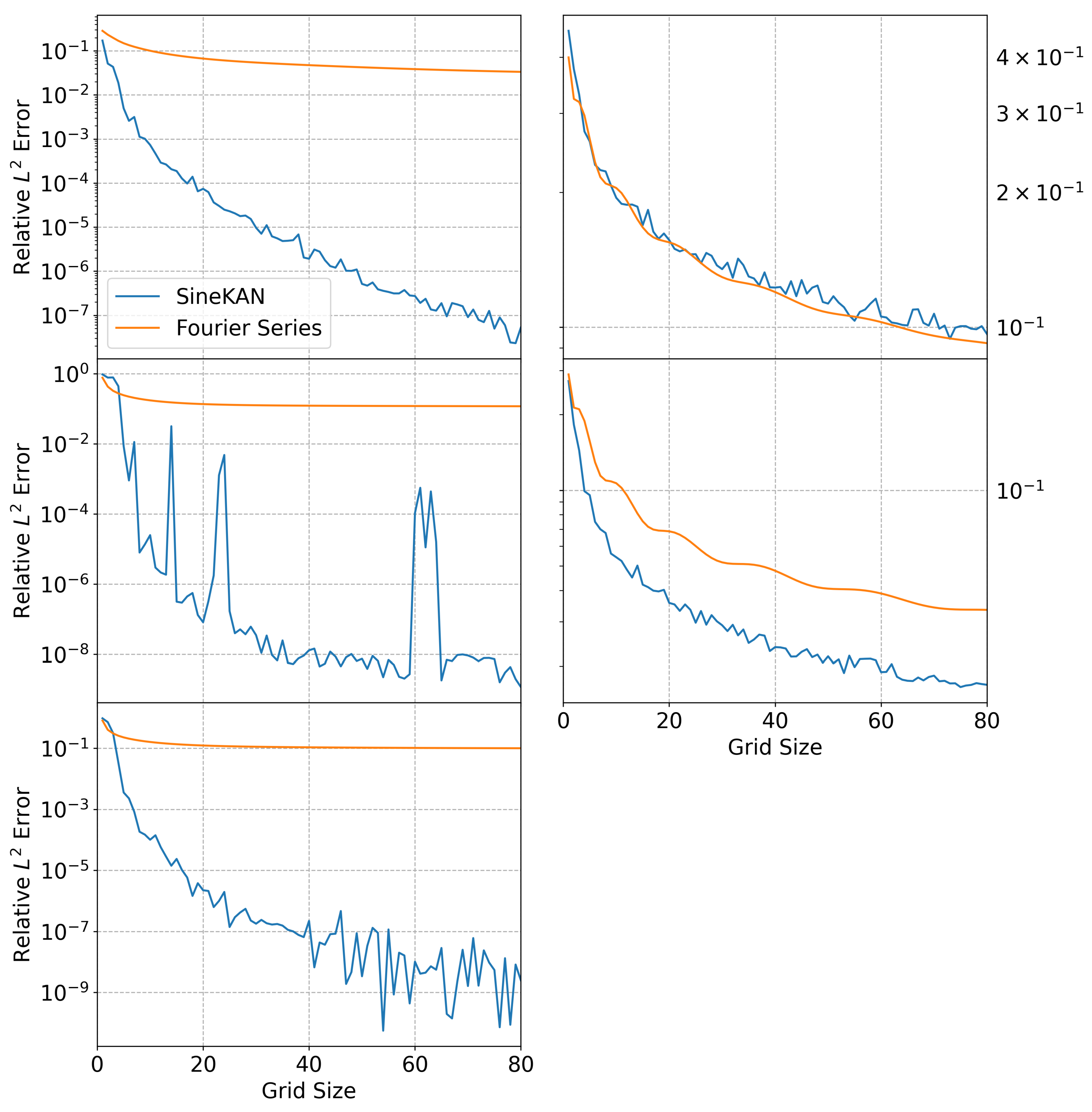
Results for 1D functions are shown in Figure 1. For (19)–(21), the SineKAN approximation significantly outperforms the Fourier series approximation. In (22), performance is roughly comparable between the two. We observe that the function in (22) has less regularity, which causes both the SineKAN and the Fourier series to converge slowly.

For multi-dimensional functions, we benchmarked the following two equations on a 100 by 100 mesh grid of input values ranging from 0.01 to 1:

The first function,

$$f(x,y)=x^2+y^2-a{e}^{-{\displaystyle \frac{{(x-1)}^2+y^2}{c}}}-b{e}^{-{\displaystyle \frac{{(x+1)}^2+y^2}{d}}},$$

(24)

with parameters $a={\displaystyle \frac{3}{2}}$, $b=1$, $c=0.5$, and $d=0.5$, features Gaussian-like terms that create a complex surface, suitable for testing convergence on smooth but non-trivial landscapes.

The second function (Rosenbrock function),

$$f(x,y)={(a-x)}^2+b{(y-x^2)}^2,$$

(25)

with parameters $a=1$ and $b=2$, represents a nonlinear, non-symmetric surface, ideal for evaluating convergence in challenging multi-dimensional optimization problems.

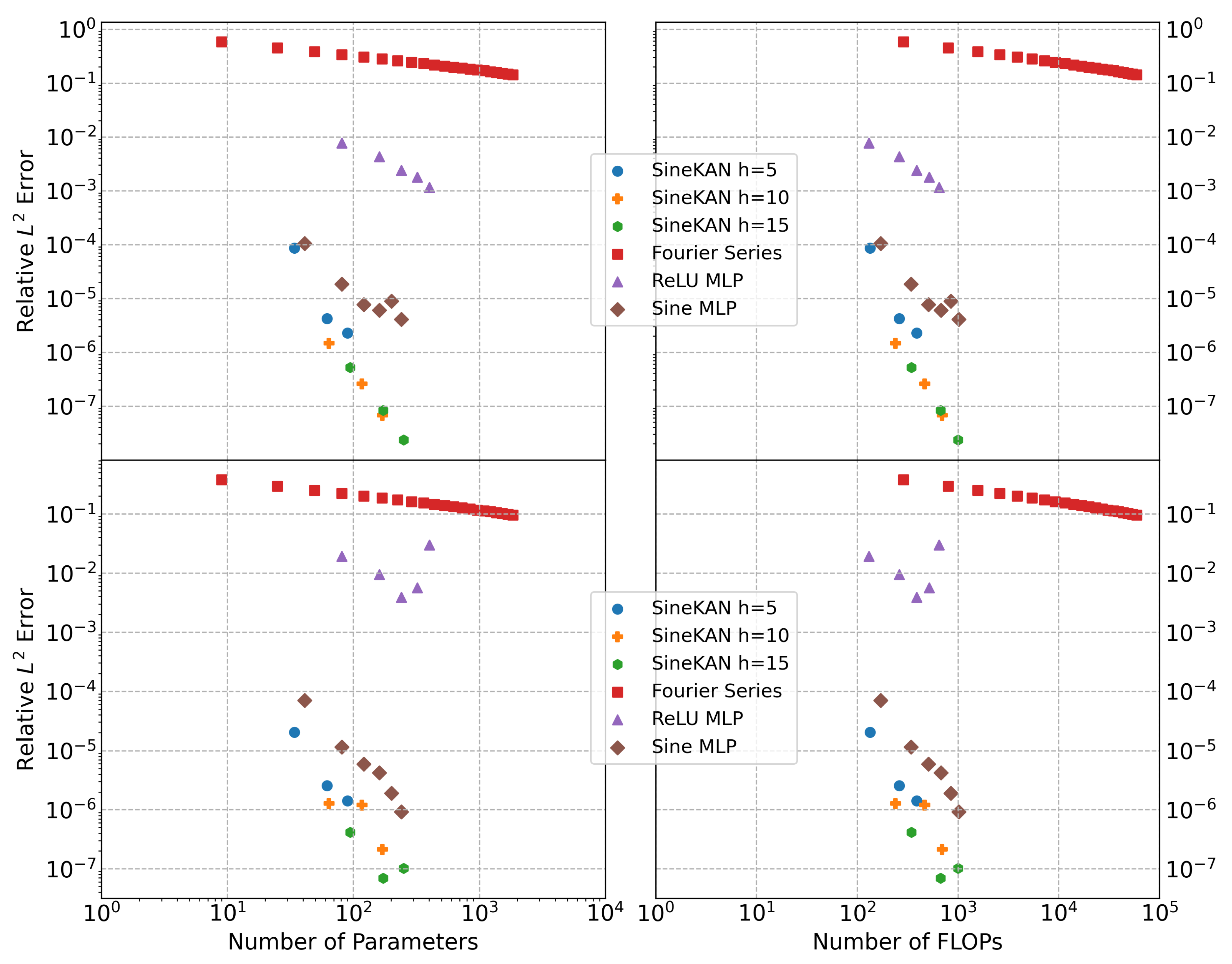
We show in Figure 2 that the two-layer SineKAN outperforms the two-layer MLP with sinusoidal activation functions as a function of the number of parameters. MLP with ReLU activations performs substantially worse, with an error several orders of magnitude higher as a function of the number of parameters and Fourier series, with a characteristic error roughly one to two orders of magnitude greater than the two-layer MLP with ReLU.

We also computed performance as a function of the number of relative FLOPs or compute units. To do this calculation, we ran 10 million iterations using numpy arrays of size 1024 to estimate the relative compute time of addition, multiplication, ReLU, and sine; we found that, when setting addition and multiplication to approximately 1 FLOP, ReLU costs an estimated 1.5 FLOPs, and sine functions cost 12 FLOPs. We carried out similar estimates in PyTorch (https://pytorch.org/, accessed on 15 September 2025) and found that the relative FLOPs for sine would be closer to 3.5 in PyTorch, and the relative FLOPs for ReLU would be around 1 FLOP. Figure 2 is based on numpy estimates.

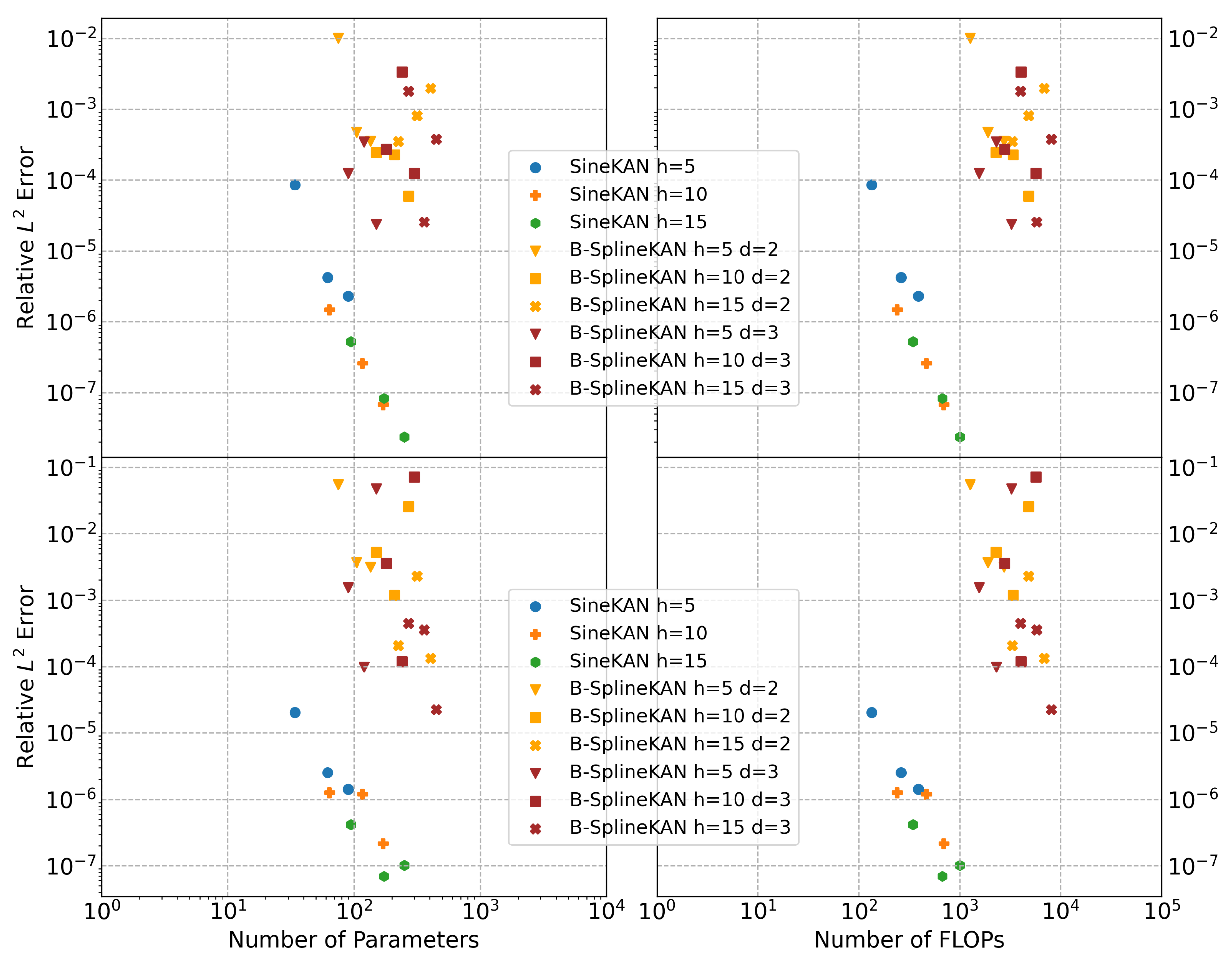
Further, in Figure 3, we show that the SineKAN model scales well compared to B-SplineKAN. The characteristic error with comparable numbers of parameters is typically two full orders of magnitude less for SineKAN, while B-SplineKAN models require substantially more FLOPs for the same number of parameters. Moreover, we find that, when compared to MLP and SineKAN models, B-SplineKAN models have significantly worse consistency in convergence with larger models’ dimensionalities, which may necessitate much more precise tuning of hyperparameters or higher-order optimization algorithms.

In

Table 3. Characteristic parameters, FLOPs, and errors for Equations (24) and (25) for best-performing models explored.

Model	Params	FLOPs	Nodes	Func. 1 Acc.	Func. 2 Acc.
MLP (ReLU)	241	391	61	2.399 × 10−3	3.916 × 10−3
KAN (B-Spline)	450	8090	169	3.786 × 10−4	2.238 × 10−5
MLP (Sine)	241	1021	61	4.083 × 10−6	9.250 × 10−7
KAN (Sine)	250	1000	73	2.343 × 10−8	1.022 × 10−7

, we show the best-performing models explored. Here, we also evaluate (for comparison) the number of nodes in the computational graphs of the models that can result in a significant bottleneck in backpropagation optimization. The characteristic error for SineKAN is substantially lower than for all other models, including the second-best MLP with sine activations, when controlling for similar numbers of parameters and FLOPs. MLP models with sine activations still achieve comparable performance that is within one to two orders of magnitude of error but require a smaller number of nodes, meaning their optimal training times could potentially be lower as a result.

5. Discussion

The original implementation of the KAN model, developed by Liu et al., used basis-spline functions [22]. These were proposed as an alternative to MLP due to their improved explainability, domain segmentation, and strong numerical performance in modeling functions. However, later work showed that, when accounting for increases in time and space complexity, the basis-spline KAN underperformed compared to MLP [27]. Previous work on the Sirens model has shown that, for function modeling, particularly for continuously differentiable functions, sinusoidal activations can improve the performance of MLP architectures [33]. This motivated the development of the SineKAN architecture, which builds on both concepts by combining the learnable on-edge activation functions and on-node weighted summation of KAN with the periodic activations from Sirens [29].

Previous work in [29,34] has established that, on tasks that require large models and with discontinuous space mappings, the SineKAN model can perform comparably to, if not better than, other commonly used fundamental machine learning models, including LSTM [12], MLP [10], and B-SplineKAN [22]. We extend these two previous works by providing a robust constructive proof for the approximation power of the SineKAN model. We show that a single layer is sufficient for the approximation of arbitrary one-dimensional functions and that a two-layer SineKAN is sufficient for the approximation of arbitrary multivariable functions bounded by the same constraints as the original KART [35].

In Figure 1, Figure 2 and Figure 3, we show that these functions can achieve low errors in modeling mathematical functions with features such as rapid- and variable-frequency oscillations. For two-dimensional D functions, we show that SineKAN outperforms MLP, including MLP with sinusoidal activations, with flexible model parameter combinations when accounting for both time and space complexity of the models. This strongly motivates further exploration of this model for numerical approximation tasks.

Given the inherent periodic nature of sinusoidal functions, our approximation framework (2) shows strong potential for modeling periodic and time-series data. Future work will explore the extension of SineKAN to continual learning tasks, particularly in scenarios involving dynamic environments or non-stationary data. Further directions include theoretical analysis of generalization bounds, integration with neural differential equations, and applications in signal processing and real-time prediction systems.

6. Conclusions

In this paper, we build upon Lorentz’s and Sprecher’s foundational work [5,6] to establish two main theorems for approximating single and multivariable functions using the sinusoidal activation function. Our proposed SineKAN models introduce learnable frequencies, amplitudes, and biases, offering a flexible and expressive framework for function approximation. Through numerical experiments, we demonstrate that SineKAN outperforms the classical Fourier series, B-SplineKAN, and MLP models in accuracy across a variety of test cases. In the task of modeling two input and one output functions, the SineKAN model achieves a characteristic relative $L^2$ error that is half an order of magnitude lower than MLP with sine activations when controlling for similar numbers of parameters and FLOPs. Compared to B-SplineKAN, this extends to roughly three orders of magnitude, and compared to MLP with ReLU activations, this extends to roughly four orders of magnitude. The SineKAN model also significantly outperforms one-dimensional and multi-dimensional Fourier transforms with the sole exception of Equation (22), where large-amplitude oscillations are densely packed near the lower bound of the domain. To support reproducibility and ease of experimentation, we provide a link to our code below.

References

1. Hilbert, D. Über die Gleichung neunten Grades. Math. Ann. 1927, 97, 243–250. [Google Scholar] [CrossRef]
2. Sternfeld, Y. Hilbert’s 13th problem and dimension. In Geometric Aspects of Functional Analysis: Israel Seminar (GAFA) 1987–1988; Springer: Berlin/Heidelberg, Germany, 1989; pp. 1–49. [Google Scholar] [CrossRef]
3. Kolmogorov, A.N. On the Representation of Continuous Functions of Several Variables by Superpositions of Continuous Functions of a Smaller Number of Variables; American Mathematical Society: Providence, RI, USA, 1961. [Google Scholar]
4. Somvanshi, S.; Javed, S.A.; Islam, M.M.; Pandit, D.; Das, S. A survey on kolmogorov-arnold network. Acm Comput. Surv. 2024, 58, 1–35. [Google Scholar] [CrossRef]
5. Lorentz, G. Approximation of functions, athena series. Sel. Top. Math. 1966, s1-43, 570–571. [Google Scholar]
6. Sprecher, D.A. On the structure of continuous functions of several variables. Trans. Am. Math. Soc. 1965, 115, 340–355. [Google Scholar] [CrossRef]
7. Rosenblatt, F. The perceptron: A probabilistic model for information storage and organization in the brain. Psychol. Rev. 1958, 65, 386. [Google Scholar] [CrossRef]
8. Minsky, M.; Papert, S.A. Perceptrons, Reissue of the 1988 Expanded Edition with a New Foreword by Léon Bottou: An Introduction to Computational Geometry; MIT Press: Cambridge, MA, USA, 2017. [Google Scholar]
9. Amari, S. A theory of adaptive pattern classifiers. IEEE Trans. Electron. Comput. 2006, EC-16, 299–307. [Google Scholar] [CrossRef]
10. Rumelhart, D.E.; Hinton, G.E.; Williams, R.J. Learning representations by back-propagating errors. Nature 1986, 323, 533–536. [Google Scholar] [CrossRef]
11. Krizhevsky, A.; Sutskever, I.; Hinton, G.E. Imagenet classification with deep convolutional neural networks. Adv. Neural Inf. Process. Syst. 2012, 25, 84–90. [Google Scholar] [CrossRef]
12. Sherstinsky, A. Fundamentals of Recurrent Neural Network (RNN) and Long Short-Term Memory (LSTM) network. Phys. D Nonlinear Phenom. 2020, 404, 132306. [Google Scholar] [CrossRef]
13. Vaswani, A.; Shazeer, N.; Parmar, N.; Uszkoreit, J.; Jones, L.; Gomez, A.N.; Kaiser, L.U.; Polosukhin, I. Attention is All you Need. In Proceedings of the Advances in Neural Information Processing Systems; Guyon, I., Luxburg, U.V., Bengio, S., Wallach, H., Fergus, R., Vishwanathan, S., Garnett, R., Eds.; Curran Associates, Inc.: Red Hook, NY, USA, 2017; Volume 30. [Google Scholar]
14. Cybenko, G. Approximation by superpositions of a sigmoidal function. Math. Control Signals Syst. 1989, 2, 303–314. [Google Scholar] [CrossRef]
15. Hornik, K.; Stinchcombe, M.; White, H. Multilayer feedforward networks are universal approximators. Neural Netw. 1989, 2, 359–366. [Google Scholar] [CrossRef]
16. Hecht-Nielsen, R. Kolmogorov’s mapping neural network existence theorem. In Proceedings of the International Conference on Neural Networks; IEEE Press: New York, NY, USA, 1987; Volume 3, pp. 11–14. [Google Scholar]
17. Hecht-Nielsen, R. Neurocomputing; Addison-Wesley Longman Publishing Co., Inc.: Boston, MA, USA, 1989. [Google Scholar]
18. Girosi, F.; Poggio, T. Representation properties of networks: Kolmogorov’s theorem is irrelevant. Neural Comput. 1989, 1, 465–469. [Google Scholar] [CrossRef]
19. Kůrková, V. Kolmogorov’s Theorem Is Relevant. Neural Comput. 1991, 3, 617–622. [Google Scholar] [CrossRef]
20. Kůrková, V. Kolmogorov’s theorem and multilayer neural networks. Neural Netw. 1992, 5, 501–506. [Google Scholar] [CrossRef]
21. Liu, Z.; Ma, P.; Wang, Y.; Matusik, W.; Tegmark, M. Kan 2.0: Kolmogorov-arnold networks meet science. arXiv 2024, arXiv:2408.10205. [Google Scholar] [CrossRef]
22. Liu, Z.; Wang, Y.; Vaidya, S.; Ruehle, F.; Halverson, J.; Soljačić, M.; Hou, T.Y.; Tegmark, M. Kan: Kolmogorov-arnold networks. arXiv 2024, arXiv:2404.19756. [Google Scholar] [PubMed]
23. Li, Z. Kolmogorov-arnold networks are radial basis function networks. arXiv 2024, arXiv:2405.06721. [Google Scholar] [CrossRef]
24. Qiu, Q.; Zhu, T.; Gong, H.; Chen, L.; Ning, H. Relu-kan: New kolmogorov-arnold networks that only need matrix addition, dot multiplication, and relu. arXiv 2024, arXiv:2406.02075. [Google Scholar]
25. Sidharth, S.S.; Keerthana, A.R.; Gokul, R.; Anas, K.P. Chebyshev polynomial-based kolmogorov-arnold networks: An efficient architecture for nonlinear function approximation. arXiv 2024, arXiv:2405.07200. [Google Scholar]
26. Xu, J.; Chen, Z.; Li, J.; Yang, S.; Wang, W.; Hu, X.; Ngai, E.C.H. FourierKAN-GCF: Fourier Kolmogorov-Arnold Network–An Effective and Efficient Feature Transformation for Graph Collaborative Filtering. arXiv 2024, arXiv:2406.01034. [Google Scholar]
27. Shukla, K.; Toscano, J.D.; Wang, Z.; Zou, Z.; Karniadakis, G.E. A comprehensive and fair comparison between mlp and kan representations for differential equations and operator networks. Comput. Methods Appl. Mech. Eng. 2024, 431, 117290. [Google Scholar] [CrossRef]
28. Yu, R.; Yu, W.; Wang, X. Kan or mlp: A fairer comparison. arXiv 2024, arXiv:2407.16674. [Google Scholar] [CrossRef]
29. Reinhardt, E.; Ramakrishnan, D.; Gleyzer, S. SineKAN: Kolmogorov-Arnold Networks using sinusoidal activation functions. Front. Artif. Intell. 2025, 7, 1462952. [Google Scholar] [CrossRef]
30. Franklin, P. The Weierstrass Approximation Theorem. J. Math. Phys. 1925, 4, 148–152. [Google Scholar] [CrossRef]
31. Householder, A.S. A theory of steady-state activity in nerve-fiber networks: I. Definitions and preliminary lemmas. Bull. Math. Biophys. 1941, 3, 63–69. [Google Scholar] [CrossRef]
32. Coleman, T.F.; Li, Y. An Interior Trust Region Approach for Nonlinear Minimization Subject to Bounds. SIAM J. Optim. 1996, 6, 418–445. [Google Scholar] [CrossRef]
33. Sitzmann, V.; Martel, J.N.P.; Bergman, A.W.; Lindell, D.B.; Wetzstein, G. Implicit Neural Representations with Periodic Activation Functions. arXiv 2020, arXiv:2006.09661. [Google Scholar] [CrossRef]
34. Shamim, M.A.; Reinhardt, E.A.F.; Chowdhury, T.A.; Gleyzer, S.; Araujo, P.T. Probing Quantum Spin Systems with Kolmogorov-Arnold Neural Network Quantum States. arXiv 2025, arXiv:2506.01891. [Google Scholar] [CrossRef]
35. Kolmogorov, A.N. On the representations of continuous functions of many variables by superposition of continuous functions of one variable and addition. Dokl. Akad. Nauk USSR 1957, 114, 953–956. Available online: https://cs.uwaterloo.ca/~y328yu/classics/Kolmogorov56.pdf (accessed on 15 September 2025).
Figure 1. Approximation error as a function of grid size: Top left: Equation (19); middle left: Equation (20); bottom left: Equation (21); top right: Equation (22); middle right: Equation (23).
Mathematics 13 03157 g001
Figure 2. Approximation error of SineKAN, MLP, and Fourier series models as a function of the number of parameters (Left) and FLOPs (Right) for Equation (24) (Top) and Equation (25) (Bottom).
Mathematics 13 03157 g002
Figure 3. Approximation error of SineKAN and B-SplineKAN models as a function of the number of parameters (Left) and FLOPs (Right) for Equation (24) (Top) and Equation (25) (Bottom).
Mathematics 13 03157 g003