The Implicit Phase-Fitted and Amplification-Fitted Four-Point Block Methods for Oscillatory First-Order Problems

Abstract

This study introduces a family of implicit four-point block methods for solving first-order initial value problems (IVPs) with oscillatory solutions. In addition to an eighth-order block method, amplification-fitted and phase-fitted implicit block methods are also derived. The methods are implemented in a predictor–corrector framework, where the predictor is a four-point explicit block method constructed with the corresponding properties. A comprehensive stability analysis is carried out to assess the robustness of the proposed approaches. Comparative evaluations with existing methods demonstrate the superior efficiency of the new algorithms. Numerical experiments further confirm that the proposed techniques provide significant improvements over traditional methods, particularly for oscillatory IVPs.

1. Introduction

The ordinary differential equations (ODEs) are powerful mathematical tools that can be used to describe and analyze various real-world phenomena. Regarding processes that display periodic or cyclic behavior, examples include mechanical vibrations, electrical circuits, and biological rhythms that are often modeled using differential equations with oscillatory solutions. These formulations commonly include sinusoidal or related periodic terms, where capturing the oscillations with high accuracy is critical for reliable analysis of natural phenomena. The repetitive nature of these equations typically necessitates specialized numerical methods for their solution, making this a significant area of study [1]. Among the classical strategies for solving initial value problems (IVPs), Runge–Kutta (RK) schemes stand out as the most extensively adopted. Furthermore, several specialized classes of RK methods have been proposed on the basis of exponential fitting, trigonometrically fitted schemes, and hybrid methods [2,3,4,5,6,7,8,9,10] in the literature to enhance the accuracy of oscillatory problem solving. Implicit methods are more stable for oscillatory IVPs, allowing for larger time steps and better handling of stiffness compared to explicit methods. For a comprehensive overview of various method classes, readers can refer to the works of Butcher [11] and Hairer et al. [12]. These traditional methods compute numerical solutions sequentially, one point at a time. Instead of progressing point by point, efficiency may be enhanced through schemes that determine solutions at multiple locations concurrently through an approach identified as the block method. Several researchers have developed block methods for numerically solving first-order ordinary differential equations (ODEs), including notable contributions from Birta et al. [13], Chu and Hamilton [14], Shampine and Watt [15], and Tam et al. [16]. The following key insights from prior work underpin our study:

• Gragg and Stetter [17] employed hybrid multistep methods to address stiff systems, while Milne [18] introduced block methods that improve computational efficiency through parallelism.
• To enhance stability, hybrid block methods were later developed and optimized [19]. These approaches primarily focus on minimizing local truncation errors but are less effective for highly oscillatory problems.
• In high-frequency oscillatory problems, accurately capturing the amplitude, energy, envelope, and especially phase over long time intervals is crucial yet difficult. Real-time applications often accept phase and amplification errors in exchange for larger time steps and improved efficiency.
• Most existing numerical methods assume near-linearity, which limits their applicability. Block methods, on the other hand, are well suited for nonlinear problems and are thus more adaptable to real-world applications.

Although considerable research has been devoted to block methods, there is still a lack of approaches that efficiently control phase lag and amplification error, particularly in the context of first-order initial value problems (IVPs). In this study, we present a numerical integrator designed to solve IVPs of the form

$${\displaystyle \frac{du}{dt}}=f(t,u),u\left(t_0\right)=u_0,$$

(1)

where $t\in [t_0,t_N],u^{\prime }\left(t\right)$ denotes the system’s rate of change, $f(t,u)$ describes the system’s dynamics, and $u\left(t_0\right)=u_0$ serves as the initial condition. Within this framework, zero-stable implicit and explicit block methods are developed, and the associated theory to evaluate phase lag and amplification error (or amplification factor) [7] is employed. In addition, we introduce systematic approaches for the construction of amplification-fitted and phase-fitted block methods.

The structure of this paper is outlined as follows:

• Section 2 derives an implicit zero-stable four-point block method of order eight and an explicit zero-stable four-point block method of order four. The derivation employs the framework in [7] to evaluate the phase lag and amplification error (or amplification factor) associated with block methods for solving first-order IVPs.
• Section 3 develops strategies to optimize phase lag and amplification factor, leading to the construction of phase-fitted and amplification-fitted block methods. In particular, we present procedures for minimizing phase lag, techniques for deriving amplification-fitted schemes, and an integrated approach for constructing methods that are both phase- and amplification-fitted.
• Section 4 provides a detailed stability analysis of the proposed family of methods, examining their behavior under various conditions.
• Section 5 reports numerical experiments illustrating the accuracy and effectiveness of the proposed approaches when applied in predictor–corrector mode.

2. 4-Points Block Methods

As stated by Fatunla [20], the difference equation in matrix form for the s-point m-step block method in solving an initial value problem (IVP) (1) is given by

$$U_n=\sum _{i=1}^m{A}_i{U}_{n-i}+h\sum _{i=0}^m{B}_i{F}_{n-i},$$

(2)

where

$$U_n=\left[\begin{array}{c}{u}_{ns}\\ u_{ns+1}\\ \dots \\ u_{ns+s-1}\end{array}\right]\mathrm{and}{F}_n=\left[\begin{array}{c}{f}_{ns}\\ f_{ns+1}\\ \dots \\ f_{ns+s-1}\end{array}\right],$$

where $n=0,1,2,\dots ,$ and $f_{ns}=f(t_0+h\left(ns\right),u_{ns}).$

In the classification of block schemes, the method is considered explicit if the coefficient matrix $B_0$ vanishes, $B_0=0$; otherwise, it is an implicit method. According to [21,22,23], assuming u is smooth, the local truncation error for the block method (2) results from the Taylor expansion of the linear difference operator L and is expressed as

$$L[u\left(t\right);h]=h^{0}u\left(t\right)C_0+h^1{u}^{\prime }\left(t\right)C_1+h^2{u}^{″}\left(t\right)C_2+\cdots +h^p{u}^{\left(p\right)}\left(t\right)C_p+\dots .$$

The block method achieves an order p if and only if $C_0=C_1=C_2=\cdots =C_p=0$ and $C_{p+1}\ne 0$, where $C_{p+1}$ represents the error constant.

For the four-point one-step block method ($s=4$), the corresponding matrix finite difference equation is given by

$$U_{n+1}=A{U}_n+h{B}_1{F}_n+h{B}_2{F}_{n+1},$$

(3)

with the coefficient matrices specified as

$$A=\left[\begin{array}{cccc}A\left[11\right]& A\left[12\right]& A\left[13\right]& A\left[14\right]\\ A\left[21\right]& A\left[22\right]& A\left[23\right]& A\left[24\right]\\ A\left[31\right]& A\left[32\right]& A\left[33\right]& A\left[34\right]\\ A\left[41\right]& A\left[42\right]& A\left[43\right]& A\left[44\right]\end{array}\right].$$

The property of zero stability guarantees that numerical errors remain bounded and are not amplified as the solution evolves step by step. Consequently, for a zero-stable one-step block method, all eigenvalues of A must lie within or on the unit circle in the complex plane, and any eigenvalue with a magnitude equal to 1 must have an algebraic multiplicity of 1. Several instances meet this condition for A, and one of them is given as

$$A=\left[\begin{array}{cccc}{\displaystyle \frac{1}{10}}& {\displaystyle \frac{1}{5}}& {\displaystyle \frac{3}{10}}& {\displaystyle \frac{2}{5}}\\ {\displaystyle \frac{1}{10}}& {\displaystyle \frac{1}{5}}& {\displaystyle \frac{3}{10}}& {\displaystyle \frac{2}{5}}\\ {\displaystyle \frac{1}{10}}& {\displaystyle \frac{1}{5}}& {\displaystyle \frac{3}{10}}& {\displaystyle \frac{2}{5}}\\ {\displaystyle \frac{1}{10}}& {\displaystyle \frac{1}{5}}& {\displaystyle \frac{3}{10}}& {\displaystyle \frac{2}{5}}\end{array}\right].$$

(4)

2.1. Implicit Block Method

Considering matrix A given in (4), a zero-stable four-point implicit block method

$$U_{n+1}=A{U}_n+h{W}_2{F}_n+h{W}_3{F}_{n+1},$$

(5)

is derived as follows: By using Taylor series, the difference equation

$$U_{n+1}-A{U}_n-h{W}_2{F}_n-h{W}_3{F}_{n+1}$$

is expanded, and enforcing zero coefficients for $u^{\prime }\left(t\right),u^{″}\left(t\right),\dots ,u^{\left(8\right)}\left(t\right)$ across the rows generates a system of 32 equations with 32 unknowns, wherein solving it using MATHEMATICA (Version number: 11.0.1.0), gives the following matrix

$$W_2=\left[\begin{array}{cccc}{\displaystyle \frac{3287}{120960}}& {\displaystyle \frac{138469}{604800}}& {\displaystyle \frac{8013}{22400}}& {\displaystyle \frac{116213}{120960}}\\ {\displaystyle \frac{1739}{60480}}& {\displaystyle \frac{64937}{302400}}& {\displaystyle \frac{14027}{33600}}& {\displaystyle \frac{47993}{60480}}\\ {\displaystyle \frac{3127}{120960}}& {\displaystyle \frac{144869}{604800}}& {\displaystyle \frac{7213}{22400}}& {\displaystyle \frac{122869}{120960}}\\ {\displaystyle \frac{2251}{60480}}& {\displaystyle \frac{44057}{302400}}& {\displaystyle \frac{7449}{11200}}& {\displaystyle \frac{17161}{60480}}\end{array}\right],W_3=\left[\begin{array}{cccc}{\displaystyle \frac{55397}{120960}}& -{\displaystyle \frac{167}{4480}}& {\displaystyle \frac{3061}{604800}}& -{\displaystyle \frac{221}{604800}}\\ {\displaystyle \frac{13709}{12096}}& {\displaystyle \frac{2951}{6720}}& -{\displaystyle \frac{8927}{302400}}& {\displaystyle \frac{767}{302400}}\\ {\displaystyle \frac{92293}{120960}}& {\displaystyle \frac{5721}{4480}}& {\displaystyle \frac{221141}{604800}}& -{\displaystyle \frac{763}{86400}}\\ {\displaystyle \frac{107713}{60480}}& {\displaystyle \frac{121}{448}}& {\displaystyle \frac{460193}{302400}}& {\displaystyle \frac{12761}{43200}}\end{array}\right].$$

2.2. Explicit Block Method

We follow the above procedure to find the coefficient matrix for the zero-stable four-point explicit block method via

$$U_{n+1}=A{U}_n+h{W}_4{F}_n.$$

(6)

The difference Equation (6), when expanded using Taylor’s expansion and with vanishing coefficients of $u^{\prime }\left(t\right),u^{″}\left(t\right),\dots ,u^{iv}\left(t\right)$, yields 16 equations in 16 unknowns. These equations can then be solved using MATHEMATICA, yielding the following matrix:

$$W_4=\left[\begin{array}{cccc}-{\displaystyle \frac{13}{40}}& {\displaystyle \frac{199}{120}}& -{\displaystyle \frac{221}{120}}& {\displaystyle \frac{301}{120}}\\ -{\displaystyle \frac{157}{60}}& {\displaystyle \frac{209}{20}}& -{\displaystyle \frac{281}{20}}& {\displaystyle \frac{553}{60}}\\ -{\displaystyle \frac{373}{40}}& {\displaystyle \frac{4199}{120}}& -{\displaystyle \frac{5461}{120}}& {\displaystyle \frac{2861}{120}}\\ -{\displaystyle \frac{479}{20}}& {\displaystyle \frac{5207}{60}}& -{\displaystyle \frac{6523}{60}}& {\displaystyle \frac{3053}{60}}\end{array}\right].$$

The implicit block method (5) has the following local truncation error:

$$LTE=\left[\begin{array}{c}-{\displaystyle \frac{649u^{\left(9\right)}\left(t\right)h^9}{3628800}}+O\left(h^{10}\right)\\ -{\displaystyle \frac{647u^{\left(9\right)}\left(t\right)h^9}{604800}}+O\left(h^{10}\right)\\ {\displaystyle \frac{683u^{\left(9\right)}\left(t\right)h^9}{725760}}+O\left(h^{10}\right)\\ -{\displaystyle \frac{15269u^{\left(9\right)}\left(t\right)h^9}{1814400}}+O\left(h^{10}\right)\end{array}\right],$$

and for the explicit block method (6), we have

$$LTE=\left[\begin{array}{c}{\displaystyle \frac{241}{720}}{u}^{\left(5\right)}\left(t\right)h^5+O\left(h^6\right)\\ {\displaystyle \frac{119}{40}}{u}^{\left(5\right)}\left(t\right)h^5+O\left(h^6\right)\\ {\displaystyle \frac{8873}{720}}{u}^{\left(5\right)}\left(t\right)h^5+O\left(h^6\right)\\ {\displaystyle \frac{13067}{360}}{u}^{\left(5\right)}\left(t\right)h^5+O\left(h^6\right)\end{array}\right].$$

The implicit method is of order eight, while the explicit method has an accuracy of order four. To analyze the phase lag and amplification factor of the four-point one-step block method (3), consider the following test equation:

$$u^{\prime }\left(t\right)=i\omega u\left(t\right),$$

(7)

which has an analytical solution given as

$$u\left(t\right)=exp\left(i\omega t\right),$$

(8)

Using the theory presented in [7], we assess it for the block methods (3). After applying the block method to the IVP (7), the following result is obtained:

$$\left[\begin{array}{c}{u}_{n+4}\\ u_{n+5}\\ u_{n+6}\\ u_{n+7}\end{array}\right]=A\left[\begin{array}{c}{u}_n\\ u_{n+1}\\ u_{n+2}\\ u_{n+3}\end{array}\right]+h\left(i\omega \right)B_1\left[\begin{array}{c}{u}_n\\ u_{n+1}\\ u_{n+2}\\ u_{n+3}\end{array}\right]+h\left(i\omega \right)B_2\left[\begin{array}{c}{u}_{n+4}\\ u_{n+5}\\ u_{n+6}\\ u_{n+7}\end{array}\right].$$

(9)

Further, considering $\eta =\omega h$, the system of difference Equation (9) possesses the following characteristic equation:

$$\left[\begin{array}{c}{\zeta }^4\\ {\zeta }^5\\ {\zeta }^6\\ {\zeta }^7\end{array}\right]-A\left[\begin{array}{c}1\\ {\zeta }^1\\ {\zeta }^2\\ {\zeta }^3\end{array}\right]-i\eta B_1\left[\begin{array}{c}1\\ {\zeta }^1\\ {\zeta }^2\\ {\zeta }^3\end{array}\right]-i\eta B_2\left[\begin{array}{c}{\zeta }^4\\ {\zeta }^5\\ {\zeta }^6\\ {\zeta }^7\end{array}\right].$$

(10)

Holding ${\zeta }^n={exp}^{ni\psi \left(\eta \right)}=\cos \left(n\psi \left(\eta \right)\right)+i\sin \left(n\psi \left(\eta \right)\right),n\in \mathbb{N}$, the above equation arrives at

$$(I-i\eta B_2)\left[\begin{array}{c}\cos \left(4\psi \right(\eta \left)\right)+i\sin \left(4\psi \right(\eta \left)\right)\\ \cos \left(5\psi \right(\eta \left)\right)+i\sin \left(5\psi \right(\eta \left)\right)\\ \cos \left(6\psi \right(\eta \left)\right)+i\sin \left(6\psi \right(\eta \left)\right)\\ \cos \left(7\psi \right(\eta \left)\right)+i\sin \left(7\psi \right(\eta \left)\right)\end{array}\right]=(A+i\eta B_1)\left[\begin{array}{c}1\\ \cos \left(\psi \right(\eta \left)\right)+i\sin \left(\psi \right(\eta \left)\right)\\ \cos \left(2\psi \right(\eta \left)\right)+i\sin \left(2\psi \right(\eta \left)\right)\\ \cos \left(3\psi \right(\eta \left)\right)+i\sin \left(3\psi \right(\eta \left)\right)\end{array}\right].$$

(11)

Definition 1 

(Order of Phase Lag). Let the theoretical solution of the scalar test Equation (7) at $t=h$ be expressed as $\exp \left(i\omega h\right)$, or equivalently, $\exp \left(i\eta \right)$. The corresponding numerical solution at $t=h$, obtained from the scalar test Equation (7), is given by $\exp \left(i\psi \right(\eta \left)\right)$. The phase lag is then defined by the following expression:

$$\mathrm{\Phi }=\eta -\psi \left(\eta \right).$$

(12)

If the phase lag Φ asymptotically behaves as $\mathcal{O}\left({\eta }^{q+1}\right)$ as $\eta \to 0$, the phase lag is said to have an order of q.

Lemma 1. 

The relations provided below hold as

$$\begin{array}{cc}\hfill \cos \left(j\psi \right(\eta \left)\right)& =\cos \left(j\eta \right)+c{j}^2{\eta }^{q+2}+\mathcal{O}\left({\eta }^{q+4}\right),\hfill \\ \hfill \sin \left(j\psi \right(\eta \left)\right)& =\sin \left(j\eta \right)-cj{\eta }^{q+1}+\mathcal{O}\left({\eta }^{q+3}\right).\hfill \end{array}$$

(13)

Proof. 

See Ref. [7] for the detailed proof.  □

Theorem 1. 

(Amplification Factor): The amplification factor $AF$ for a four-point one-step block method (3) is given by

$$AF=-{\eta }^{q+1}C=K^{-1}.\left(\left[\begin{array}{c}\sin \left(4\eta \right)\\ \sin \left(5\eta \right)\\ \sin \left(6\eta \right)\\ \sin \left(7\eta \right)\end{array}\right]-A.\left[\begin{array}{c}0\\ \sin \left(\eta \right)\\ \sin \left(2\eta \right)\\ \sin \left(3\eta \right)\end{array}\right]-\eta B_1.\left[\begin{array}{c}1\\ \cos \left(\eta \right)\\ \cos \left(2\eta \right)\\ \cos \left(3\eta \right)\end{array}\right]-\eta B_2.\left[\begin{array}{c}\cos \left(4\eta \right)\\ \cos \left(5\eta \right)\\ \cos \left(6\eta \right)\\ \cos \left(7\eta \right)\end{array}\right]\right),$$

(14)

where q is the order of the amplification factor, which is defined as

$$K=-\left[\begin{array}{cccc}4& 0& 0& 0\\ 0& 5& 0& 0\\ 0& 0& 6& 0\\ 0& 0& 0& 7\end{array}\right]+A\left[\begin{array}{cccc}0& 0& 0& 0\\ 0& 1& 0& 0\\ 0& 0& 2& 0\\ 0& 0& 0& 3\end{array}\right]-{\eta }^2{B}_1\left[\begin{array}{cccc}0& 0& 0& 0\\ 0& 1^2& 0& 0\\ 0& 0& 2^2& 0\\ 0& 0& 0& 3^2\end{array}\right]-{\eta }^2{B}_2\left[\begin{array}{cccc}{4}^2& 0& 0& 0\\ 0& 5^2& 0& 0\\ 0& 0& 6^2& 0\\ 0& 0& 0& 7^2\end{array}\right]$$

and $\eta =\omega h$.

Proof. 

By applying the relation (13) derived from Lemma 1 directly into the characteristic Equation (11), we obtain the following result:

$$\begin{array}{c}\hfill (I-i\eta B_2)\left[\begin{array}{c}\cos \left(4\eta \right)+c_1{\left(4\right)}^2{\eta }^{q+2}+i(\sin \left(4\eta \right)-c_1\left(4\right){\eta }^{q+1})\\ \cos \left(5\eta \right)+c_2{\left(5\right)}^2{\eta }^{q+2}+i(\sin \left(5\eta \right)-c_2\left(5\right){\eta }^{q+1})\\ \cos \left(6\eta \right)+c_3{\left(6\right)}^2{\eta }^{q+2}+i(\sin \left(6\eta \right)-c_3\left(6\right){\eta }^{q+1})\\ \cos \left(7\eta \right)+c_4{\left(7\right)}^2{\eta }^{q+2}+i(\sin \left(7\eta \right)-c_4\left(7\right){\eta }^{q+1})\end{array}\right]\\ \hfill =(A+i\eta B_1)\left[\begin{array}{c}1\\ \cos \left(\eta \right)+c_2{\left(1\right)}^2{\eta }^{q+2}+i(\sin \left(\eta \right)-c_2\left(1\right){\eta }^{q+1})\\ \cos \left(2\eta \right)+c_3{\left(2\right)}^2{\eta }^{q+2}+i(\sin \left(2\eta \right)-c_3\left(2\right){\eta }^{q+1})\\ \cos \left(3\eta \right)+c_4{\left(3\right)}^2{\eta }^{q+2}+i(\sin \left(3\eta \right)-c_4\left(3\right){\eta }^{q+1})\end{array}\right],\end{array}$$

(15)

The imaginary component of the system presented above is expressed as

$$\begin{array}{cc}\hfill & \left[\begin{array}{c}\sin \left(4\eta \right)-c_1\left(4\right){\eta }^{q+1}\\ \sin \left(5\eta \right)-c_2\left(5\right){\eta }^{q+1}\\ \sin \left(6\eta \right)-c_3\left(6\right){\eta }^{q+1}\\ \sin \left(7\eta \right)-c_4\left(7\right){\eta }^{q+1}\end{array}\right]-\eta B_2\left[\begin{array}{c}\cos \left(4\eta \right)+c_1{\left(4\right)}^2{\eta }^{q+2}\\ \cos \left(5\eta \right)+c_2{\left(5\right)}^2{\eta }^{q+2}\\ \cos \left(6\eta \right)+c_3{\left(6\right)}^2{\eta }^{q+2}\\ \cos \left(7\eta \right)+c_4{\left(7\right)}^2{\eta }^{q+2}\end{array}\right]\hfill \\ \hfill & =A\left[\begin{array}{c}0\\ \sin \left(\eta \right)-c_2\left(1\right){\eta }^{q+1}\\ \sin \left(2\eta \right)-c_3\left(2\right){\eta }^{q+1}\\ \sin \left(3\eta \right)-c_4\left(3\right){\eta }^{q+1}\end{array}\right]+\eta B_1\left[\begin{array}{c}1\\ \cos \left(\eta \right)+c_2{\left(1\right)}^2{\eta }^{q+2}\\ \cos \left(2\eta \right)+c_3{\left(2\right)}^2{\eta }^{q+2}\\ \cos \left(3\eta \right)+c_4{\left(3\right)}^2{\eta }^{q+2}\end{array}\right],\hfill \end{array}$$

which can be further simplified as

$$\begin{array}{cc}\hfill & -{\eta }^{q+1}\left(\left[\begin{array}{cccc}4& 0& 0& 0\\ 0& 5& 0& 0\\ 0& 0& 6& 0\\ 0& 0& 0& 7\end{array}\right]-A\left[\begin{array}{cccc}0& 0& 0& 0\\ 0& 1& 0& 0\\ 0& 0& 2& 0\\ 0& 0& 0& 3\end{array}\right]\right)C\hfill \\ \hfill & -{\eta }^{q+1}\left({\eta }^2{B}_1\left[\begin{array}{cccc}0& 0& 0& 0\\ 0& 1^2& 0& 0\\ 0& 0& 2^2& 0\\ 0& 0& 0& 3^2\end{array}\right]+{\eta }^2{B}_2\left[\begin{array}{cccc}{4}^2& 0& 0& 0\\ 0& 5^2& 0& 0\\ 0& 0& 6^2& 0\\ 0& 0& 0& 7^2\end{array}\right]\right)C\hfill \\ \hfill & =-\left[\begin{array}{c}\sin \left(4\eta \right)\\ \sin \left(5\eta \right)\\ \sin \left(6\eta \right)\\ \sin \left(7\eta \right)\end{array}\right]+A\left[\begin{array}{c}0\\ \sin \left(\eta \right)\\ \sin \left(2\eta \right)\\ \sin \left(3\eta \right)\end{array}\right]+\eta B_1\left[\begin{array}{c}1\\ \cos \left(\eta \right)\\ \cos \left(2\eta \right)\\ \cos \left(3\eta \right)\end{array}\right]+\eta B_2\left[\begin{array}{c}\cos \left(4\eta \right)\\ \cos \left(5\eta \right)\\ \cos \left(6\eta \right)\\ \cos \left(7\eta \right)\end{array}\right],\hfill \end{array}$$

(16)

where $C={[c_1,c_2,c_3,c_4]}^T$. The explicit formula for calculating the amplification factor ($AF$) of the block method (3) is

$$-{\eta }^{q+1}C=K^{-1}.\left(\left[\begin{array}{c}\sin \left(4\eta \right)\\ \sin \left(5\eta \right)\\ \sin \left(6\eta \right)\\ \sin \left(7\eta \right)\end{array}\right]-A.\left[\begin{array}{c}0\\ \sin \left(\eta \right)\\ \sin \left(2\eta \right)\\ \sin \left(3\eta \right)\end{array}\right]-\eta B_1.\left[\begin{array}{c}1\\ \cos \left(\eta \right)\\ \cos \left(2\eta \right)\\ \cos \left(3\eta \right)\end{array}\right]-\eta B_2.\left[\begin{array}{c}\cos \left(4\eta \right)\\ \cos \left(5\eta \right)\\ \cos \left(6\eta \right)\\ \cos \left(7\eta \right)\end{array}\right]\right),$$

(17)

where $K=-\left[\begin{array}{cccc}4& 0& 0& 0\\ 0& 5& 0& 0\\ 0& 0& 6& 0\\ 0& 0& 0& 7\end{array}\right]+A\left[\begin{array}{cccc}0& 0& 0& 0\\ 0& 1& 0& 0\\ 0& 0& 2& 0\\ 0& 0& 0& 3\end{array}\right]$

$-{\eta }^2{B}_1\left[\begin{array}{cccc}0& 0& 0& 0\\ 0& 1^2& 0& 0\\ 0& 0& 2^2& 0\\ 0& 0& 0& 3^2\end{array}\right]-{\eta }^2{B}_2\left[\begin{array}{cccc}{4}^2& 0& 0& 0\\ 0& 5^2& 0& 0\\ 0& 0& 6^2& 0\\ 0& 0& 0& 7^2\end{array}\right]$.

• □

Theorem 2. 

(Phase Lag): The phase lag $PhEr$ for a four-point one-step block method (3) is calculated as

$$PhEr=-{\eta }^{q+2}C=L^{-1}.\left(\left[\begin{array}{c}\cos \left(4\eta \right)\\ \cos \left(5\eta \right)\\ \cos \left(6\eta \right)\\ \cos \left(7\eta \right)\end{array}\right]-A.\left[\begin{array}{c}1\\ \cos \left(\eta \right)\\ \cos \left(2\eta \right)\\ \cos \left(3\eta \right)\end{array}\right]+\eta B_1.\left[\begin{array}{c}0\\ \sin \left(\eta \right)\\ \sin \left(2\eta \right)\\ \sin \left(3\eta \right)\end{array}\right]+\eta B_2.\left[\begin{array}{c}\sin \left(4\eta \right)\\ \sin \left(5\eta \right)\\ \sin \left(6\eta \right)\\ \sin \left(7\eta \right)\end{array}\right]\right),$$

(18)

where q is the order of phase lag

$$L=\left[\begin{array}{cccc}{4}^2& 0& 0& 0\\ 0& 5^2& 0& 0\\ 0& 0& 6^2& 0\\ 0& 0& 0& 7^2\end{array}\right]-A\left[\begin{array}{cccc}0& 0& 0& 0\\ 0& 1^2& 0& 0\\ 0& 0& 2^2& 0\\ 0& 0& 0& 3^2\end{array}\right]-B_1\left[\begin{array}{cccc}0& 0& 0& 0\\ 0& 1& 0& 0\\ 0& 0& 2& 0\\ 0& 0& 0& 3\end{array}\right]-B_2\left[\begin{array}{cccc}4& 0& 0& 0\\ 0& 5& 0& 0\\ 0& 0& 6& 0\\ 0& 0& 0& 7\end{array}\right]$$

and $\eta =\omega h$.

Proof. 

In a manner analogous to the proof of Theorem 1, we apply Lemma 1 and substitute the resulting relation (13) into the characteristic Equation (10), thereby deriving (15). Similarly, by examining the real part of (15), one obtains

$$\begin{array}{cc}\hfill \left[\begin{array}{c}\cos \left(4\eta \right)+c_1{\left(4\right)}^2{\eta }^{q+2}\\ \cos \left(5\eta \right)+c_2{\left(5\right)}^2{\eta }^{q+2}\\ \cos \left(6\eta \right)+c_3{\left(6\right)}^2{\eta }^{q+2}\\ \cos \left(7\eta \right)+c_4{\left(7\right)}^2{\eta }^{q+2}\end{array}\right]=& A\left[\begin{array}{c}1\\ \cos \left(\eta \right)+c_2{\left(1\right)}^2{\eta }^{q+2}\\ \cos \left(2\eta \right)+c_3{\left(2\right)}^2{\eta }^{q+2}\\ \cos \left(3\eta \right)+c_4{\left(3\right)}^2{\eta }^{q+2}\end{array}\right]-\eta B_1\left[\begin{array}{c}0\\ \sin \left(\eta \right)-c_2\left(1\right){\eta }^{q+1}\\ \sin \left(2\eta \right)-c_3\left(2\right){\eta }^{q+1}\\ \sin \left(3\eta \right)-c_4\left(3\right){\eta }^{q+1}\end{array}\right]\hfill \\ \hfill & -\eta B_2\left[\begin{array}{c}\sin \left(4\eta \right)-c_1\left(4\right){\eta }^{q+1}\\ \sin \left(5\eta \right)-c_2\left(5\right){\eta }^{q+1}\\ \sin \left(6\eta \right)-c_3\left(6\right){\eta }^{q+1}\\ \sin \left(7\eta \right)-c_4\left(7\right){\eta }^{q+1}\end{array}\right].\hfill \\ \hfill \end{array}$$

(19)

$$\begin{array}{cc}\hfill & -{\eta }^{q+2}\left(\left[\begin{array}{cccc}{4}^2& 0& 0& 0\\ 0& 5^2& 0& 0\\ 0& 0& 6^2& 0\\ 0& 0& 0& 7^2\end{array}\right]-A\left[\begin{array}{cccc}0& 0& 0& 0\\ 0& 1^2& 0& 0\\ 0& 0& 2^2& 0\\ 0& 0& 0& 3^2\end{array}\right]-B_1\left[\begin{array}{cccc}0& 0& 0& 0\\ 0& 1& 0& 0\\ 0& 0& 2& 0\\ 0& 0& 0& 3\end{array}\right]-B_2\left[\begin{array}{cccc}4& 0& 0& 0\\ 0& 5& 0& 0\\ 0& 0& 6& 0\\ 0& 0& 0& 7\end{array}\right]\right)C\hfill \\ \hfill & =\left[\begin{array}{c}\cos \left(4\eta \right)\\ \cos \left(5\eta \right)\\ \cos \left(6\eta \right)\\ \cos \left(7\eta \right)\end{array}\right]-A\left[\begin{array}{c}1\\ \cos \left(\eta \right)\\ \cos \left(2\eta \right)\\ \cos \left(3\eta \right)\end{array}\right]+\eta B_1\left[\begin{array}{c}0\\ \sin \left(\eta \right)\\ \sin \left(2\eta \right)\\ \sin \left(3\eta \right)\end{array}\right]+\eta B_2\left[\begin{array}{c}\sin \left(4\eta \right)\\ \sin \left(5\eta \right)\\ \sin \left(6\eta \right)\\ \sin \left(7\eta \right)\end{array}\right],\hfill \\ \hfill \end{array}$$

(20)

$$\begin{array}{cc}\hfill & -{\eta }^{q+2}C=L^{-1}\left(\left[\begin{array}{c}\cos \left(4\eta \right)\\ \cos \left(5\eta \right)\\ \cos \left(6\eta \right)\\ \cos \left(7\eta \right)\end{array}\right]-A\left[\begin{array}{c}1\\ \cos \left(\eta \right)\\ \cos \left(2\eta \right)\\ \cos \left(3\eta \right)\end{array}\right]+\eta B_1\left[\begin{array}{c}0\\ \sin \left(\eta \right)\\ \sin \left(2\eta \right)\\ \sin \left(3\eta \right)\end{array}\right]+\eta B_2\left[\begin{array}{c}\sin \left(4\eta \right)\\ \sin \left(5\eta \right)\\ \sin \left(6\eta \right)\\ \sin \left(7\eta \right)\end{array}\right]\right),\hfill \\ \hfill \end{array}$$

(21)

where $L=\left[\begin{array}{cccc}{4}^2& 0& 0& 0\\ 0& 5^2& 0& 0\\ 0& 0& 6^2& 0\\ 0& 0& 0& 7^2\end{array}\right]-A\left[\begin{array}{cccc}0& 0& 0& 0\\ 0& 1^2& 0& 0\\ 0& 0& 2^2& 0\\ 0& 0& 0& 3^2\end{array}\right]-B_1\left[\begin{array}{cccc}0& 0& 0& 0\\ 0& 1& 0& 0\\ 0& 0& 2& 0\\ 0& 0& 0& 3\end{array}\right]-B_2\left[\begin{array}{cccc}4& 0& 0& 0\\ 0& 5& 0& 0\\ 0& 0& 6& 0\\ 0& 0& 0& 7\end{array}\right]$.

• □

To calculate the order of the amplification factor of the implicit block method (5), Formula (14) from Theorem 1 for the implicit method (5) is expanded with $B_1=W_2$ and $B_2=W_3$, using the Taylor series expansion, as follows:

$$AF=\left[\begin{array}{c}{\displaystyle \frac{649{\eta }^9}{7257600}}+O\left({\eta }^{10}\right)\\ {\displaystyle \frac{647{\eta }^9}{1814400}}+O\left({\eta }^{10}\right)\\ -{\displaystyle \frac{683{\eta }^9}{2903040}}+O\left({\eta }^{10}\right)\\ {\displaystyle \frac{15269{\eta }^9}{9072000}}+O\left({\eta }^{10}\right)\end{array}\right].$$

Thus, $q=8$, indicating that the implicit block method (5) has an eighth-order amplification factor. Similarly, the phase error for (5) is obtained by applying Taylor’s expansion to the direct Formula (18) from Theorem 2, with $B_1=W_2$ and $B_2=W_3$, resulting in

$$PhEr=\left[\begin{array}{c}{\displaystyle \frac{2767{\eta }^{10}}{39916800}}+O\left({\eta }^{11}\right)\\ {\displaystyle \frac{13067{\eta }^{10}}{36288000}}+O\left({\eta }^{11}\right)\\ -{\displaystyle \frac{4039{\eta }^{10}}{16070400}}+O\left({\eta }^{11}\right)\\ {\displaystyle \frac{116363{\eta }^{10}}{79833600}}+O\left({\eta }^{11}\right)\end{array}\right].$$

Thus, $q=8$, and the block method (5), referred to as $Im1$, exhibits an eighth-order phase lag.

Similarly, for the explicit block method (6), using the Formula (14) with $B_1=W_4$ and setting $B_2$ as the zero matrix, the amplification factor is of fourth order and is given by

$$AF=\left[\begin{array}{c}-{\displaystyle \frac{241{\eta }^5}{1440}}+O\left({\eta }^7\right)\\ -{\displaystyle \frac{119{\eta }^5}{120}}+O\left({\eta }^7\right)\\ -{\displaystyle \frac{8873{\eta }^5}{2880}}+O\left({\eta }^7\right)\\ -{\displaystyle \frac{13067{\eta }^5}{1800}}+O\left({\eta }^7\right)\end{array}\right],$$

and the phase lag error evaluated as

$$PhEr=\left[\begin{array}{c}-{\displaystyle \frac{943{\eta }^6}{7920}}+O\left({\eta }^8\right)\\ -{\displaystyle \frac{4511{\eta }^6}{7200}}+O\left({\eta }^8\right)\\ -{\displaystyle \frac{40223{\eta }^6}{22320}}+O\left({\eta }^8\right)\\ -{\displaystyle \frac{5773{\eta }^6}{1440}}+O\left({\eta }^8\right)\end{array}\right].$$

So, the explicit block method (6), denoted as $E1$, has a phase lag of order four.

2.3. Method 2: Amplification-Fitted Block Method with Minimal Phase Lag

The modified four-point one-step block method is derived by preserving the property of zero stability to ensure the accuracy and stability of the numerical solution. To derive the amplification-fitted block method with minimal phase lag, we begin by considering the matrix A from (4) in conjunction with the direct formula provided in (14). The method follows the steps outlined in the algorithm below.

Algorithm:

• Eliminate the amplification factor: Eliminate the amplification factor and solve the set of equations for unknown coefficients and using the coefficients obtained, calculate the phase lag.
• Perform Taylor series expansion: Expand the calculated phase lag using a Taylor series to obtain a set of relations of unknown coefficients.
• Minimize the phase lag: Solve the system of equations required to adjust the parameters such that the phase lag is minimized. Similarly, minimize the local truncation error, making use of the updated coefficients derived.

2.3.1. Implicit Amplification-Fitted Method

By following the algorithm, eliminating the amplification factor $AF$ from the block method (3), where the matrix A is defined as in (4), and $B_l\left[ij\right]$ denotes the element of $B_l$ at the ith row and jth column, results in a set of equations that are used to adjust the method for minimal phase lag:

$$\begin{array}{cc}\hfill B_2\left[14\right]=& -\left({\displaystyle \frac{\sec \left(7\eta \right)}{10\eta }}\right)(10B_1\left[11\right]\eta +10B_1\left[12\right]\eta \cos \left(\eta \right)+10B_1\left[13\right]\eta \cos \left(2\eta \right)\hfill \\ \hfill & +10B_1\left[14\right]\eta \cos \left(3\eta \right)+10B_2\left[11\right]\eta \cos \left(4\eta \right)+10B_2\left[12\right]\eta \cos \left(5\eta \right)\hfill \\ \hfill & +10B_2\left[13\right]\eta \cos \left(6\eta \right)+2\sin \left(\eta \right)+3\sin \left(2\eta \right)+4\sin \left(3\eta \right)-10\sin \left(4\eta \right)),\hfill \\ \hfill B_2\left[24\right]=& \left(-{\displaystyle \frac{\sec \left(7\eta \right)}{10\eta }}\right)(10B_1\left[21\right]\eta +10B_1\left[22\right]\eta \cos \left(\eta \right)+10B_1\left[23\right]\eta \cos \left(2\eta \right)\hfill \\ \hfill & +10B_1\left[24\right]\eta \cos \left(3\eta \right)+10B_2\left[21\right]\eta \cos \left(4\eta \right)+10B_2\left[22\right]\eta \cos \left(5\eta \right)\hfill \\ \hfill & +10B_2\left[23\right]\eta \cos \left(6\eta \right)+2\sin \left(\eta \right)+3\sin \left(2\eta \right)+4\sin \left(3\eta \right)-10\sin \left(5\eta \right)),\hfill \\ \hfill B_2\left[34\right]=& -{\displaystyle \frac{\sec \left(7\eta \right)}{10\eta }}(10B_1\left[32\right]\eta \cos \left(\eta \right)+10B_1\left[33\right]\eta \cos \left(2\eta \right)+10B_1\left[34\right]\eta \cos \left(3\eta \right)\hfill \\ \hfill & +10B_1\left[31\right]\eta +10B_2\left[32\right]\eta \cos \left(5\eta \right)+10B_2\left[33\right]\eta \cos \left(6\eta \right)+10B_2\left[31\right]\eta \cos \left(4\eta \right)\hfill \\ \hfill & +2\sin \left(\eta \right)+3\sin \left(2\eta \right)+4\sin \left(3\eta \right)-10\sin \left(6\eta \right)),\hfill \\ \hfill \end{array}$$

$$\begin{array}{cc}\hfill B_2\left[44\right]=& -{\displaystyle \frac{\sec \left(7\eta \right)}{10\eta }}(10B_1\left[41\right]\eta +10B_1\left[42\right]\eta \cos \left(\eta \right)+10B_1\left[43\right]\eta \cos \left(2\eta \right)\hfill \\ \hfill & +10B_1\left[44\right]\eta \cos \left(3\eta \right)+10B_2\left[41\right]\eta \cos \left(4\eta \right)+10B_2\left[42\right]\eta \cos \left(5\eta \right)\hfill \\ \hfill & +10B_2\left[43\right]\eta \cos \left(6\eta \right)+2\sin \left(\eta \right)+3\sin \left(2\eta \right)+4\sin \left(3\eta \right)-10\sin \left(7\eta \right)).\hfill \end{array}$$

(22)

Furthermore, the phase lag is assessed using the coefficient values mentioned above and then minimized by eliminating the coefficients of ${\eta }^2$, ${\eta }^4$, ${\eta }^6$,${\eta }^8$,${\eta }^{10}$, and ${\eta }^{12}$. The obtained values are subsequently substituted to compute the local truncation error, aiming to eliminate the coefficient of $h^3$, which gives the following matrix:

$$B_2=\left[\begin{array}{cccc}{\displaystyle \frac{391775819}{1016064000}}& {\displaystyle \frac{163100597}{9144576000}}& -{\displaystyle \frac{55351181}{3048192000}}& B_2\left[14\right]\\ {\displaystyle \frac{492367847}{508032000}}& {\displaystyle \frac{2567326361}{4572288000}}& -{\displaystyle \frac{122195153}{1524096000}}& B_2\left[24\right]\\ {\displaystyle \frac{112504477}{145152000}}& {\displaystyle \frac{237257413}{186624000}}& {\displaystyle \frac{159746357}{435456000}}& B_2\left[34\right]\\ {\displaystyle \frac{557146087}{508032000}}& {\displaystyle \frac{3499920601}{4572288000}}& {\displaystyle \frac{2014586927}{1524096000}}& B_2\left[44\right]\end{array}\right],$$

where

$$\begin{array}{cc}\hfill B_2\left[14\right]=& {\displaystyle \frac{55351181\cos \left(6\eta \right)\sec \left(7\eta \right)}{3048192000}}-{\displaystyle \frac{163100597\cos \left(5\eta \right)\sec \left(7\eta \right)}{9144576000}}-{\displaystyle \frac{2639859331\cos \left(\eta \right)\sec \left(7\eta \right)}{11176704000}}\hfill \\ \hfill & -{\displaystyle \frac{6650747869\cos \left(2\eta \right)\sec \left(7\eta \right)}{20118067200}}-{\displaystyle \frac{25595901389\cos \left(3\eta \right)\sec \left(7\eta \right)}{25147584000}}-{\displaystyle \frac{2649041539\sec \left(7\eta \right)}{100590336000}}\hfill \\ \hfill & -{\displaystyle \frac{\left(\frac{391775819\eta \cos \left(4\eta \right)}{101606400}+2\sin \left(\eta \right)+3\sin \left(2\eta \right)+4\sin \left(3\eta \right)-10\sin \left(4\eta \right)\right)\sec \left(7\eta \right)}{10\eta }},\hfill \\ \hfill B_2\left[24\right]=& {\displaystyle \frac{122195153\cos \left(6\eta \right)\sec \left(7\eta \right)}{1524096000}}-{\displaystyle \frac{118177373\cos \left(\eta \right)\sec \left(7\eta \right)}{508032000}}-{\displaystyle \frac{492367847\cos \left(4\eta \right)\sec \left(7\eta \right)}{508032000}}\hfill \\ \hfill & -{\displaystyle \frac{322380227\cos \left(2\eta \right)\sec \left(7\eta \right)}{914457600}}-{\displaystyle \frac{1058770387\cos \left(3\eta \right)\sec \left(7\eta \right)}{1143072000}}\hfill \\ \hfill & -{\displaystyle \frac{2567326361\cos \left(5\eta \right)\sec \left(7\eta \right)}{4572288000}}-{\displaystyle \frac{121679837\sec \left(7\eta \right)}{4572288000}}\hfill \\ \hfill & -{\displaystyle \frac{\left(2\sin \right(\eta )+3\sin (2\eta )+4\sin (3\eta )-10\sin (5\eta \left)\right)\sec \left(7\eta \right)}{10\eta }},\hfill \\ \hfill B_2\left[34\right]=& -{\displaystyle \frac{112504477\cos \left(4\eta \right)\sec \left(7\eta \right)}{145152000}}-{\displaystyle \frac{237257413\cos \left(5\eta \right)\sec \left(7\eta \right)}{186624000}}\hfill \\ \hfill & -{\displaystyle \frac{135919469\cos \left(2\eta \right)\sec \left(7\eta \right)}{410572800}}\hfill \\ \hfill & -{\displaystyle \frac{159746357\cos \left(6\eta \right)\sec \left(7\eta \right)}{435456000}}-{\displaystyle \frac{377435813\cos \left(\eta \right)\sec \left(7\eta \right)}{1596672000}}\hfill \\ \hfill & -{\displaystyle \frac{3599298187\cos \left(3\eta \right)\sec \left(7\eta \right)}{3592512000}}-{\displaystyle \frac{378040997\sec \left(7\eta \right)}{14370048000}}\hfill \\ \hfill & -{\displaystyle \frac{\left(2\sin \right(\eta )+3\sin (2\eta )+4\sin (3\eta )-10\sin (6\eta \left)\right)\sec \left(7\eta \right)}{10\eta }},\hfill \\ \hfill B_2\left[44\right]=& -{\displaystyle \frac{557146087\cos \left(4\eta \right)\sec \left(7\eta \right)}{508032000}}-{\displaystyle \frac{2014586927\cos \left(6\eta \right)\sec \left(7\eta \right)}{1524096000}}\hfill \\ \hfill & -{\displaystyle \frac{755642029\cos \left(2\eta \right)\sec \left(7\eta \right)}{2011806720}}-{\displaystyle \frac{3499920601\cos \left(5\eta \right)\sec \left(7\eta \right)}{4572288000}}\hfill \\ \hfill & -{\displaystyle \frac{1275777983\cos \left(\eta \right)\sec \left(7\eta \right)}{5588352000}}-{\displaystyle \frac{1356755327\sec \left(7\eta \right)}{50295168000}}\hfill \\ \hfill & -{\displaystyle \frac{\left(\frac{10752538897\eta \cos \left(3\eta \right)}{1257379200}+2\sin \left(\eta \right)+3\sin \left(2\eta \right)+4\sin \left(3\eta \right)-10\sin \left(7\eta \right)\right)\sec \left(7\eta \right)}{10\eta }}.\hfill \\ \hfill \end{array}$$

(23)

and

$$B_1=\left[\begin{array}{cccc}{\displaystyle \frac{2649041539}{100590336000}}& {\displaystyle \frac{2639859331}{11176704000}}& {\displaystyle \frac{6650747869}{20118067200}}& {\displaystyle \frac{25595901389}{25147584000}}\\ {\displaystyle \frac{121679837}{4572288000}}& {\displaystyle \frac{118177373}{508032000}}& {\displaystyle \frac{322380227}{914457600}}& {\displaystyle \frac{1058770387}{1143072000}}\\ {\displaystyle \frac{378040997}{14370048000}}& {\displaystyle \frac{377435813}{1596672000}}& {\displaystyle \frac{135919469}{410572800}}& {\displaystyle \frac{3599298187}{3592512000}}\\ {\displaystyle \frac{1356755327}{50295168000}}& {\displaystyle \frac{1275777983}{5588352000}}& {\displaystyle \frac{755642029}{2011806720}}& {\displaystyle \frac{10752538897}{12573792000}}\end{array}\right]$$

The modified implicit block method is denoted as $Im2$ and produces the following local truncation error:

$$LTE=\left[\begin{array}{c}-{\displaystyle \frac{9380033\left(u^5\left(t\right)-w^4{u}^{\prime }\left(t\right)\right)h^5}{14370048000}}+O\left(h^6\right)\\ -{\displaystyle \frac{854239\left(u^5\left(t\right)-w^4{u}^{\prime }\left(t\right)\right)h^5}{653184000}}+O\left(h^6\right)\\ -{\displaystyle \frac{1735873\left(u^5\left(t\right)-w^4{u}^{\prime }\left(t\right)\right)h^5}{14370048000}}+O\left(h^6\right)\\ -{\displaystyle \frac{4609987\left(u^5\left(t\right)-w^4{u}^{\prime }\left(t\right)\right)h^5}{1026432000}}+O\left(h^6\right)\end{array}\right],$$

and has the following phase error

$$PhEr=\left[\begin{array}{c}-{\displaystyle \frac{116966591{\eta }^{14}}{587119104000}}+O\left({\eta }^{15}\right)\\ -{\displaystyle \frac{495782381{\eta }^{14}}{3736212480000}}+O\left({\eta }^{15}\right)\\ -{\displaystyle \frac{5472819343{\eta }^{14}}{81075810816000}}+O\left({\eta }^{15}\right)\\ -{\displaystyle \frac{341385511{\eta }^{14}}{4425974784000}}+O\left({\eta }^{15}\right)\end{array}\right].$$

2.3.2. Explicit Amplification Fitted Method

Applying the algorithm to eliminate the amplification factor $AF$ to derive the explicit block method, where the matrix A is defined as in (4) and $B_2=0$, generates following set of equations:

$$\begin{array}{cc}\hfill B_1\left[14\right]=& -B_1\left[11\right]\sec \left(3\eta \right)-B_1\left[12\right]\cos \left(\eta \right)\sec \left(3\eta \right)-B_1\left[13\right]\cos \left(2\eta \right)\sec \left(3\eta \right)\hfill \\ \hfill & -{\displaystyle \frac{\left(2\sin \right(\eta )+3\sin (2\eta )+4\sin (3\eta )-10\sin (4\eta \left)\right)\sec \left(3\eta \right)}{10\eta }},\hfill \\ \hfill B_1\left[24\right]=& -B_1\left[21\right]\sec \left(3\eta \right)-B_1\left[22\right]\cos \left(\eta \right)\sec \left(3\eta \right)-B_1\left[23\right]\cos \left(2\eta \right)\sec \left(3\eta \right)\hfill \\ \hfill & -{\displaystyle \frac{\left(2\sin \right(\eta )+3\sin (2\eta )+4\sin (3\eta )-10\sin (5\eta \left)\right)\sec \left(3\eta \right)}{10\eta }},\hfill \\ \hfill B_1\left[34\right]=& -B_1\left[32\right]\cos \left(\eta \right)\sec \left(3\eta \right)-B_1\left[33\right]\cos \left(2\eta \right)\sec \left(3\eta \right)-B_1\left[31\right]\sec \left(3\eta \right)\hfill \\ \hfill & -{\displaystyle \frac{\left(2\sin \right(\eta )+3\sin (2\eta )+4\sin (3\eta )-10\sin (6\eta \left)\right)\sec \left(3\eta \right)}{10\eta }},\hfill \\ \hfill B_1\left[44\right]=& -B_1\left[41\right]\sec \left(3\eta \right)-B_1\left[42\right]\cos \left(\eta \right)\sec \left(3\eta \right)-B_1\left[43\right]\cos \left(2\eta \right)\sec \left(3\eta \right)\hfill \\ \hfill & -{\displaystyle \frac{\left(2\sin \right(\eta )+3\sin (2\eta )+4\sin (3\eta )-10\sin (7\eta \left)\right)\sec \left(3\eta \right)}{10\eta }},\hfill \\ \hfill \end{array}$$

(24)

Subsequently, the coefficients of ${\eta }^2,{\eta }^4,$ and ${\eta }^6$ equate to zero in order to minimize phase error, wherein the following coefficient matrix is obtained:

$$B_1=\left[\begin{array}{cccc}{\displaystyle \frac{7}{288}}& {\displaystyle \frac{47}{180}}& -{\displaystyle \frac{137}{1440}}& B_1\left[14\right]\\ {\displaystyle \frac{31}{720}}& -{\displaystyle \frac{17}{90}}& -{\displaystyle \frac{541}{720}}& B_1\left[24\right]\\ -{\displaystyle \frac{413}{1440}}& -{\displaystyle \frac{209}{180}}& -{\displaystyle \frac{457}{1440}}& B_1\left[34\right]\\ -{\displaystyle \frac{469}{144}}& {\displaystyle \frac{361}{90}}& -{\displaystyle \frac{3781}{720}}& B_1\left[44\right]\end{array}\right],$$

where

$$\begin{array}{cc}\hfill B_1\left[14\right]=& {\displaystyle \frac{1}{288}}(-7)\sec \left(3\eta \right)-{\displaystyle \frac{47}{180}}\cos \left(\eta \right)\sec \left(3\eta \right)+{\displaystyle \frac{137\cos \left(2\eta \right)\sec \left(3\eta \right)}{1440}}\hfill \\ \hfill & -{\displaystyle \frac{\left(2\sin \right(\eta )+3\sin (2\eta )+4\sin (3\eta )-10\sin (4\eta \left)\right)\sec \left(3\eta \right)}{10\eta }},\hfill \\ \hfill B_1\left[24\right]=& {\displaystyle \frac{1}{720}}(-31)\sec \left(3\eta \right)+{\displaystyle \frac{17}{90}}\cos \left(\eta \right)\sec \left(3\eta \right)+{\displaystyle \frac{541}{720}}\cos \left(2\eta \right)\sec \left(3\eta \right),\hfill \\ \hfill & -{\displaystyle \frac{\left(2\sin \right(\eta )+3\sin (2\eta )+4\sin (3\eta )-10\sin (5\eta \left)\right)\sec \left(3\eta \right)}{10\eta }}\hfill \\ \hfill B_1\left[34\right]=& {\displaystyle \frac{209}{180}}\cos \left(\eta \right)\sec \left(3\eta \right)+{\displaystyle \frac{457\cos \left(2\eta \right)\sec \left(3\eta \right)}{1440}}+{\displaystyle \frac{413\sec \left(3\eta \right)}{1440}},\hfill \\ \hfill & -{\displaystyle \frac{\left(2\sin \right(\eta )+3\sin (2\eta )+4\sin (3\eta )-10\sin (6\eta \left)\right)\sec \left(3\eta \right)}{10\eta }}\hfill \\ \hfill B_1\left[44\right]=& {\displaystyle \frac{469}{144}}\sec \left(3\eta \right)-{\displaystyle \frac{361}{90}}\cos \left(\eta \right)\sec \left(3\eta \right)+{\displaystyle \frac{3781}{720}}\cos \left(2\eta \right)\sec \left(3\eta \right),\hfill \\ \hfill & -{\displaystyle \frac{\left(2\sin \right(\eta )+3\sin (2\eta )+4\sin (3\eta )-10\sin (7\eta \left)\right)\sec \left(3\eta \right)}{10\eta }}.\hfill \end{array}$$

This modified explicit method is denoted as $E2$. The method $E2$ has the following properties:

$$LTE=\left[\begin{array}{c}{\displaystyle \frac{503\left(u^{\prime }\left(t\right)w^2+u^3\left(t\right)\right)h^3}{1440}}+O\left(h^4\right)\\ {\displaystyle \frac{383}{144}}\left(u^{\prime }\left(t\right)w^2+u^3\left(t\right)\right)h^3+O\left(h^4\right)\\ {\displaystyle \frac{2603}{288}}\left(u^{\prime }\left(t\right)w^2+u^3\left(t\right)\right)h^3+O\left(h^4\right)\\ {\displaystyle \frac{14899}{720}}\left(u^{\prime }\left(t\right)w^2+u^3\left(t\right)\right)h^3+O\left(h^4\right)\end{array}\right],$$

$$PhEr=\left[\begin{array}{c}-{\displaystyle \frac{221{\eta }^8}{3326400}}+O\left({\eta }^{10}\right)\\ {\displaystyle \frac{767{\eta }^8}{3024000}}+O\left({\eta }^{10}\right)\\ -{\displaystyle \frac{763{\eta }^8}{1339200}}+O\left({\eta }^{10}\right)\\ {\displaystyle \frac{12761{\eta }^8}{950400}}+O\left({\eta }^{10}\right)\end{array}\right].$$

2.4. Method 3: Amplification-Fitted and Phase-Fitted Block Method

The method is derived through the following steps:

• Eliminate $AF$ and $PhEr$, which results in eight equations.
• Compute the local truncation error.
• Determine the remaining unknown coefficients by enhancing the precision of the local truncation error.

2.4.1. Implicit Phase-Fitted and Amplification-Fitted Block Method

Ensuring zero stability by considering A given in (4), the amplification factor $AF$ is evaluated using Formula (14), which is (A1) given in Appendix A. By eliminating the amplification error, the phase error $PhEr$ for the amplification-fitted block method is calculated from Formula (18), as given (A2) in Appendix A.

Eliminating $AF$ leads to (22), while setting $PhEr$ to zero results in the following:

$$B_1=\left[\begin{array}{cccc}{B}_1\left[11\right]& {\displaystyle \frac{138469}{604800}}& {\displaystyle \frac{8013}{22400}}& {\displaystyle \frac{116213}{120960}}\\ B_1\left[21\right]& {\displaystyle \frac{64937}{302400}}& {\displaystyle \frac{14027}{33600}}& {\displaystyle \frac{47993}{60480}}\\ B_1\left[31\right]& {\displaystyle \frac{144869}{604800}}& {\displaystyle \frac{7213}{22400}}& {\displaystyle \frac{122869}{120960}}\\ B_1\left[41\right]& {\displaystyle \frac{44057}{302400}}& {\displaystyle \frac{7449}{11200}}& {\displaystyle \frac{17161}{60480}}\end{array}\right],$$

(25)

$$B_2=\left[\begin{array}{cccc}{\displaystyle \frac{55397}{120960}}& -{\displaystyle \frac{167}{4480}}& {\displaystyle \frac{3061}{604800}}& B_2\left[14\right]\\ {\displaystyle \frac{13709}{12096}}& {\displaystyle \frac{2951}{6720}}& -{\displaystyle \frac{8927}{302400}}& B_2\left[24\right]\\ {\displaystyle \frac{92293}{120960}}& {\displaystyle \frac{5721}{4480}}& {\displaystyle \frac{221141}{604800}}& B_2\left[34\right]\\ {\displaystyle \frac{107713}{60480}}& {\displaystyle \frac{121}{448}}& {\displaystyle \frac{460193}{302400}}& B_2\left[44\right]\end{array}\right],$$

(26)

and Appendix A provides the other elements of the matrices.

The local truncation error of the block method $Im3$ is

$$LTE=\left[\begin{array}{c}{\displaystyle \frac{649\left(w^8{u}^{\prime }\left(t\right)-u^{\left(9\right)}\left(t\right)\right)h^9}{3628800}}+O\left(h^{10}\right)\\ {\displaystyle \frac{647\left(w^8{u}^{\prime }\left(t\right)-u^{\left(9\right)}\left(t\right)\right)h^9}{604800}}+O\left(h^{10}\right)\\ -{\displaystyle \frac{683\left(w^8{u}^{\prime }\left(t\right)-u^{\left(9\right)}\left(t\right)\right)h^9}{725760}}+O\left(h^{10}\right)\\ {\displaystyle \frac{15269\left(w^8{u}^{\prime }\left(t\right)-u^{\left(9\right)}\left(t\right)\right)h^9}{1814400}}+O\left(h^{10}\right)\end{array}\right].$$

Therefore, Method $Im3$ is of eighth order, with $AF=0$ and $PhEr=0$.

2.4.2. Explicit Phase-Fitted and Amplification-Fitted Block Method

To find coefficient matrix for amplification fitted and phase fitted explicit block method, $B_2$ is considered as the zero matrix, and after eliminating the amplification error, it results in the set of Equation (24). The phase error $PhEr$ is then evaluated and given (A3) in Appendix A.

With elimination of the phase error, the following set of equations are obtained:

$$\begin{array}{cc}\hfill B_1\left[13\right]=& -{\displaystyle \frac{B_1\left[11\right]\tan \left(3\eta \right)}{\cos \left(2\eta \right)\tan \left(3\eta \right)-\sin \left(2\eta \right)}}-{\displaystyle \frac{B_1\left[12\right](\cos \left(\eta \right)\tan \left(3\eta \right)-\sin \left(\eta \right))}{\cos \left(2\eta \right)\tan \left(3\eta \right)-\sin \left(2\eta \right)}}\hfill \\ \hfill & -{\displaystyle \frac{1}{10\eta \left(\sin \right(2\eta )-\cos (2\eta \left)\tan \right(3\eta \left)\right)}}[-2\cos \left(\eta \right)-3\cos \left(2\eta \right)-4\cos \left(3\eta \right)\hfill \\ \hfill & +10\cos \left(4\eta \right)-2\sin \left(\eta \right)\tan \left(3\eta \right)-3\sin \left(2\eta \right)\tan \left(3\eta \right)-4\sin \left(3\eta \right)\tan \left(3\eta \right)\hfill \\ \hfill & +10\sin \left(4\eta \right)\tan \left(3\eta \right)-1],\hfill \\ \hfill B_1\left[21\right]=& -B_1\left[22\right]\cot \left(3\eta \right)(\cos \left(\eta \right)\tan \left(3\eta \right)-\sin \left(\eta \right))-B_1\left[23\right]\cot \left(3\eta \right)(\cos \left(2\eta \right)\tan \left(3\eta \right)-\sin \left(2\eta \right))\hfill \\ \hfill & -{\displaystyle \frac{1}{10\eta }}\left[\cot \left(3\eta \right)\right(2\cos \left(\eta \right)+3\cos \left(2\eta \right)+4\cos \left(3\eta \right)-10\cos \left(5\eta \right)\hfill \\ \hfill & +2\sin \left(\eta \right)\tan \left(3\eta \right)+3\sin \left(2\eta \right)\tan \left(3\eta \right)+4\sin \left(3\eta \right)\tan \left(3\eta \right)\hfill \\ \hfill & -10\sin \left(5\eta \right)\tan \left(3\eta \right)+1\left)\right],\hfill \\ \hfill B_1\left[31\right]=& -B_1\left[32\right]\cot \left(3\eta \right)(\cos \left(\eta \right)\tan \left(3\eta \right)-\sin \left(\eta \right))-B_1\left[33\right]\cot \left(3\eta \right)(\cos \left(2\eta \right)\tan \left(3\eta \right)-\sin \left(2\eta \right))\hfill \\ \hfill & -{\displaystyle \frac{1}{10\eta }}\left[\cot \left(3\eta \right)\right(2\cos \left(\eta \right)+3\cos \left(2\eta \right)+4\cos \left(3\eta \right)-10\cos \left(6\eta \right)\hfill \\ \hfill & +2\sin \left(\eta \right)\tan \left(3\eta \right)+3\sin \left(2\eta \right)\tan \left(3\eta \right)+4\sin \left(3\eta \right)\tan \left(3\eta \right)-10\sin \left(6\eta \right)\tan \left(3\eta \right)+1\left)\right],\hfill \\ \hfill B_1\left[41\right]=& -B_1\left[42\right]\cot \left(3\eta \right)(\cos \left(\eta \right)\tan \left(3\eta \right)-\sin \left(\eta \right))\hfill \\ \hfill & -B_1\left[43\right]\cot \left(3\eta \right)(\cos \left(2\eta \right)\tan \left(3\eta \right)-\sin \left(2\eta \right))\hfill \\ \hfill & -{\displaystyle \frac{1}{10\eta }}\left[\cot \left(3\eta \right)\right(2\cos \left(\eta \right)+3\cos \left(2\eta \right)+4\cos \left(3\eta \right)-10\cos \left(7\eta \right)\hfill \\ \hfill & +2\sin \left(\eta \right)\tan \left(3\eta \right)+3\sin \left(2\eta \right)\tan \left(3\eta \right)+4\sin \left(3\eta \right)\tan \left(3\eta \right)\hfill \\ \hfill & -10\sin \left(7\eta \right)\tan \left(3\eta \right)+1\left)\right],\hfill \end{array}$$

(27)

and optimizing the local truncation error, other unknown elements of the coefficient matrix are obtained, and they are given in Appendix A. The method is labeled as $E3$ and holds the following properties:

$$LTE=\left[\begin{array}{c}-{\displaystyle \frac{241}{720}}\left(w^4{u}^{\prime }\left(t\right)-u^{\left(5\right)}\left(t\right)\right)h^5+O\left(h^6\right)\\ -{\displaystyle \frac{119}{40}}\left(w^4{u}^{\prime }\left(t\right)-u^{\left(5\right)}\left(t\right)\right)h^5+O\left(h^6\right)\\ -{\displaystyle \frac{8873}{720}}\left(w^4{u}^{\prime }\left(t\right)-u^{\left(5\right)}\left(t\right)\right)h^5+O\left(h^6\right)\\ -{\displaystyle \frac{13067}{360}}\left(w^4{u}^{\prime }\left(t\right)-u^{\left(5\right)}\left(t\right)\right)h^5+O\left(h^6\right)\end{array}\right],$$

$$PhEr=0,$$

$$AF=0.$$

2.5. Method 4: Amplification-Fitted and Phase-Fitted Block Method with Vanished First Derivative of Phase Error

For this method, the first derivative of phase error is also taken into account. Even if a method has zero phase lag at a specific frequency or step size, a non-zero first derivative implies that small deviations can cause the phase error to grow rapidly. By ensuring that the first derivative of the phase error vanishes, we enhance the robustness and accuracy of the method across a broader frequency range, not just at a single point. This is particularly beneficial in long-term integration of oscillatory problems, where the frequency may vary slightly over time or be imperfectly known. The procedure is executed through the following steps:

• Evaluate the amplification factor (AF) and the phase error (PhEr).
• Compute the first derivative of the phase error.
• Repeat analogous steps to construct the block method, ensuring that the amplification factor, phase error, and its derivative are all nullified.
• Determine the remaining undetermined coefficients by optimizing the local truncation error (LTE).

2.5.1. Implicit Amplification- and Phase-Fitted Block Method with Vanished First Derivative of Phase Error

Starting with the first step outlined in the algorithm above, the system of equations given in (A1) is obtained. Eliminating the amplification factor (AF) from this system yields Equation (22). Using the resulting coefficient values, the phase error (PhEr) is then evaluated, leading to Equation (A2). Differentiating this expression with respect to $\eta$ and proceeding with the subsequent steps—namely, the elimination of the phase error and its derivative while also taking the local truncation error (LTE) into account—results in the following coefficient matrices:

$$B_1=\left[\begin{array}{cccc}{B}_1\left[11\right]& {\displaystyle \frac{138469}{604800}}& {\displaystyle \frac{8013}{22400}}& {\displaystyle \frac{116213}{120960}}\\ B_1\left[21\right]& {\displaystyle \frac{64937}{302400}}& {\displaystyle \frac{14027}{33600}}& {\displaystyle \frac{47993}{60480}}\\ B_1\left[31\right]& {\displaystyle \frac{144869}{604800}}& {\displaystyle \frac{7213}{22400}}& {\displaystyle \frac{122869}{120960}}\\ B_1\left[41\right]& {\displaystyle \frac{44057}{302400}}& {\displaystyle \frac{7449}{11200}}& {\displaystyle \frac{17161}{60480}}\end{array}\right],$$

$$B_2=\left[\begin{array}{cccc}{\displaystyle \frac{55397}{120960}}& -{\displaystyle \frac{167}{4480}}& B_2\left[13\right]& B_2\left[14\right]\\ {\displaystyle \frac{13709}{12096}}& {\displaystyle \frac{2951}{6720}}& B_2\left[23\right]& B_2\left[24\right]\\ {\displaystyle \frac{92293}{120960}}& {\displaystyle \frac{5721}{4480}}& B_2\left[33\right]& B_2\left[34\right]\\ {\displaystyle \frac{107713}{60480}}& {\displaystyle \frac{121}{448}}& B_2\left[43\right]& B_2\left[44\right]\end{array}\right].$$

Appendix A lists the values of the matrix elements, and the method labeled as $Im4$ local truncation error of the method $Im4$ is

$$LTE=\left[\begin{array}{c}{\displaystyle \frac{\left(-8165u^{\prime }\left(t\right)w^8-16602u^{\left(3\right)}\left(t\right)w^6-8437u^{\left(9\right)}\left(t\right)\right)h^9}{47174400}}+O\left(h^{10}\right)\\ {\displaystyle \frac{\left(-17723u^{\prime }\left(t\right)w^8-26134u^{\left(3\right)}\left(t\right)w^6-8411u^{\left(9\right)}\left(t\right)\right)h^9}{7862400}}+O\left(h^{10}\right)\\ {\displaystyle \frac{\left(125243u^{\prime }\left(t\right)w^8+169638u^{\left(3\right)}\left(t\right)w^6+44395u^{\left(9\right)}\left(t\right)\right)h^9}{47174400}}+O\left(h^{10}\right)\\ {\displaystyle \frac{\left(-38437u^{\prime }\left(t\right)w^8-53706u^{\left(3\right)}\left(t\right)w^6-15269u^{\left(9\right)}\left(t\right)\right)h^9}{1814400}}+O\left(h^{10}\right)\end{array}\right],$$

$$AF=0,$$

$$PhEr=0.$$

2.5.2. Explicit Amplification- and Phase-Fitted Block Method with Vanished First Derivative of Phase Error

When $B_2$ is a zero matrix and the above algorithm is applied, the first step leads to Equations (24) and (27). Consequently, the following coefficient matrix is obtained:

$$B_1=\left[\begin{array}{cccc}-{\displaystyle \frac{13}{40}}& B_1\left[12\right]& B_1\left[13\right]& B_1\left[14\right]\\ B_1\left[21\right]& {\displaystyle \frac{209}{20}}& B_1\left[23\right]& B_1\left[24\right]\\ B_1\left[31\right]& {\displaystyle \frac{4199}{120}}& B_1\left[33\right]& B_1\left[34\right]\\ B_1\left[41\right]& {\displaystyle \frac{5207}{60}}& B_1\left[43\right]& B_1\left[44\right]\end{array}\right].$$

The values of the matrix elements are provided in Appendix A, and the method denoted as $E4$ local truncation error of the method $E4$ is

$$LTE=\left[\begin{array}{c}{\displaystyle \frac{\left(461u^{\prime }\left(t\right)w^4+943u^{\left(3\right)}\left(t\right)w^2+482u^{\left(5\right)}\left(t\right)\right)h^5}{1440}}+O\left(h^6\right)\\ {\displaystyle \frac{\left(2726u^{\prime }\left(t\right)w^4+4511u^{\left(3\right)}\left(t\right)w^2+1785u^{\left(5\right)}\left(t\right)\right)h^5}{600}}+O\left(h^6\right)\\ {\displaystyle \frac{19\left(4016u^{\prime }\left(t\right)w^4+6351u^{\left(3\right)}\left(t\right)w^2+2335u^{\left(5\right)}\left(t\right)\right)h^5}{3600}}+O\left(h^6\right)\\ {\displaystyle \frac{\left(125174u^{\prime }\left(t\right)w^4+190509u^{\left(3\right)}\left(t\right)w^2+65335u^{\left(5\right)}\left(t\right)\right)h^5}{1800}}+O\left(h^6\right)\end{array}\right],$$

$$AF=0,$$

$$PhEr=0.$$

2.6. Method 5: Amplification-Fitted and Phase-Fitted Block Method with Vanished First Derivative of Amplification Factor

The procedure is carried out through the following steps:

• The amplification factor (AF) and phase error (PhEr) are first evaluated.
• Next, the first derivative of the amplification factor is computed.
• Formulate the block method, ensuring the elimination of the phase error, amplification factor, and its first-order derivative.
• Finally, the remaining undetermined coefficients are obtained by minimizing the local truncation error (LTE).

2.6.1. Implicit Amplification- and Phase-Fitted Block Method with Vanished First Derivative of Amplification Error

As a result of this algorithmic procedure, the coefficient matrices $B_1\&B_2$ are obtained. The detailed closed-form expression for elements of the matrices can be found in Appendix A. The method is referred as $Im5$.

$$B_1=\left[\begin{array}{cccc}{B}_1\left[11\right]& {\displaystyle \frac{138469}{604800}}& B_1\left[13\right]& {\displaystyle \frac{116213}{120960}}\\ B_1\left[21\right]& {\displaystyle \frac{64937}{302400}}& {\displaystyle \frac{14027}{33600}}& B_1\left[24\right]\\ B_1\left[31\right]& {\displaystyle \frac{144869}{604800}}& {\displaystyle \frac{7213}{22400}}& B_1\left[34\right]\\ B_1\left[41\right]& {\displaystyle \frac{44057}{302400}}& {\displaystyle \frac{7449}{11200}}& B_1\left[44\right]\end{array}\right],$$

$$B_2=\left[\begin{array}{cccc}{\displaystyle \frac{55397}{120960}}& -{\displaystyle \frac{167}{4480}}& {\displaystyle \frac{3061}{604800}}& B_2\left[14\right]\\ {\displaystyle \frac{13709}{12096}}& {\displaystyle \frac{2951}{6720}}& -{\displaystyle \frac{8927}{302400}}& B_2\left[24\right]\\ {\displaystyle \frac{92293}{120960}}& {\displaystyle \frac{5721}{4480}}& {\displaystyle \frac{221141}{604800}}& B_2\left[34\right]\\ {\displaystyle \frac{107713}{60480}}& {\displaystyle \frac{121}{448}}& {\displaystyle \frac{460193}{302400}}& B_2\left[44\right]\end{array}\right].$$

2.6.2. Explicit Amplification- and Phase-Fitted Block Method with Vanished First Derivative of Amplification Error

Considering $B_2=O$, the zero matrix, the algorithmic procedure yields the coefficient matrix $B_1$. The end analytical formulations of this matrix are provided in Appendix A. The method is denoted as $E5$.

$$B_1=\left[\begin{array}{cccc}{B}_1\left[11\right]& {\displaystyle \frac{199}{120}}& B_1\left[13\right]& B_1\left[14\right]\\ B_1\left[21\right]& {\displaystyle \frac{209}{20}}& B_1\left[23\right]& B_1\left[24\right]\\ B_1\left[31\right]& {\displaystyle \frac{4199}{120}}& B_1\left[33\right]& B_1\left[34\right]\\ B_1\left[41\right]& {\displaystyle \frac{5207}{60}}& B_1\left[43\right]& B_1\left[44\right]\end{array}\right],$$

The local truncation error of the method $Im5$ is

$$LTE=\left[\begin{array}{c}-{\displaystyle \frac{649\left(3u^{\prime }\left(t\right)w^8+4u^{\left(3\right)}\left(t\right)w^6+u^{\left(9\right)}\left(t\right)\right)h^9}{3628800}}+O\left(h^{10}\right)\\ -{\displaystyle \frac{647\left(3u^{\prime }\left(t\right)w^8+4u^{\left(3\right)}\left(t\right)w^6+u^{\left(9\right)}\left(t\right)\right)h^9}{604800}}+O\left(h^{10}\right)\\ {\displaystyle \frac{683\left(3u^{\prime }\left(t\right)w^8+4u^{\left(3\right)}\left(t\right)w^6+u^{\left(9\right)}\left(t\right)\right)h^9}{725760}}+O\left(h^{10}\right)\\ -{\displaystyle \frac{15269\left(3u^{\prime }\left(t\right)w^8+4u^{\left(3\right)}\left(t\right)w^6+u^{\left(9\right)}\left(t\right)\right)h^9}{1814400}}+O\left(h^{10}\right)\end{array}\right],$$

The local truncation error of the method $E5$ is

$$LTE=\left[\begin{array}{c}{\displaystyle \frac{241}{720}}\left(u^{\prime }\left(t\right)w^4+2u^{\left(3\right)}\left(t\right)w^2+u^{\left(5\right)}\left(t\right)\right)h^5+O\left(h^6\right)\\ {\displaystyle \frac{119}{40}}\left(u^{\prime }\left(t\right)w^4+2u^{\left(3\right)}\left(t\right)w^2+u^{\left(5\right)}\left(t\right)\right)h^5+O\left(h^6\right)\\ {\displaystyle \frac{8873}{720}}\left(u^{\prime }\left(t\right)w^4+2u^{\left(3\right)}\left(t\right)w^2+u^{\left(5\right)}\left(t\right)\right)h^5+O\left(h^6\right)\\ {\displaystyle \frac{13067}{360}}\left(u^{\prime }\left(t\right)w^4+2u^{\left(3\right)}\left(t\right)w^2+u^{\left(5\right)}\left(t\right)\right)h^5+O\left(h^6\right)\end{array}\right],$$

$$AF=0,$$

$$PhEr=0.$$

Table 1 comprehensively encapsulates the essential properties of the developed methods, highlighting their strengths and distinguishing features.

Table 1. Outline of key properties.

Method	Order	AF	PhEr	Vanished First-Order Derivative of AF	Vanished First-Order Derivative of PhEr
$Im1$	8	8	8	×	×
$Im2$	4	0	12	×	×
$Im3$	8	0	0	×	×
$Im4$	8	0	0	×	✓
$Im5$	8	0	0	✓	×
$E1$	4	4	4	×	×
$E2$	2	0	6	×	×
$E3$	4	0	0	×	×
$E4$	4	0	0	×	✓
$E5$	4	0	0	✓	×

3. Stability

The stability analysis helps us to understand how the method behaves under different step sizes and parameter values, ensuring that the numerical solution remains bounded and converges to the correct solution, even for large or small values of the step size h.

3.1. Explicit Block Methods

For the family of explicit block methods, a general formulation (3) is adopted in which the coefficient matrix A is specified as in (4), the matrix $B_2$ is identically zero, and $B_1$ is non-zero matrix and is applied to the scalar test problem $u^{\prime }=\lambda u$, with $\lambda \in \mathbb{C}$, where it reduces to the following difference equation:

$$U_{n+1}=(A+\widehat{h}{B}_1)U_n,\mathrm{where}\widehat{h}=\lambda h.$$

(28)

The characteristic polynomial of the method, as derived from Equation (28), is given by

$$k^4+T_1\left(\widehat{h}\right)k^3+T_2\left(\widehat{h}\right)k^2+T_3\left(\widehat{h}\right)k+T_4=0.$$

The stability polynomial is solved for $\widehat{h}$, subject to the condition $\left|k\right|\le 1$, using MATHEMATICA, and the resulting regions in the complex plane illustrate the method’s stability characteristics. This analysis reveals the influence of step size and parameter $\eta$ (for methods $E2$–$E5$) on overall stability.

3.2. Implicit Block Methods

Considering a general form (3) for implicit block method that incorporates the non-zero coefficients A, $B_1$, and $B_2$, with the corresponding function evaluations at different time steps, is applied to the scalar test equation $u^{\prime }=\lambda u$, with $\lambda \in \mathbb{C}$, the method results in the following difference equation:

$$(I-\widehat{h}{B}_2)U_{n+1}=(A+\widehat{h}{B}_1)U_n,\mathrm{where}\widehat{h}=\lambda h.$$

(29)

The characteristic polynomial for this method, derived from Equation (29), is

$$k^4+S_1\left(\widehat{h}\right)k^3+S_2\left(\widehat{h}\right)k^2+S_3\left(\widehat{h}\right)k+S_4=0.$$

Stability regions in the complex plane are obtained from the stability polynomial $\left|k\right|\le 1$, utilizing MATHEMATICA, and examined for various step sizes and parameter values, $\eta$ for the $Im2$–$Im5$ methods. Figure 1, Figure 2, Figure 3, Figure 4, Figure 5, Figure 6, Figure 7, Figure 8, Figure 9, Figure 10, Figure 11, Figure 12, Figure 13, Figure 14, Figure 15, Figure 16, Figure 17, Figure 18, Figure 19, Figure 20, Figure 21, Figure 22, Figure 23, Figure 24, Figure 25 and Figure 26 depict these regions for the derived explicit and implicit block methods, showing that the implicit variants consistently exhibit larger stability domains than their explicit counterparts.

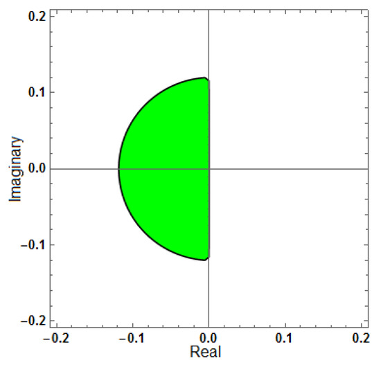
Figure 1. Region of stability for $E1$ (explicit method).

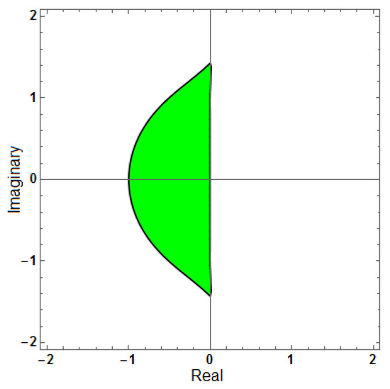
Figure 2. Region of stability for $Im1$ (implicit method).

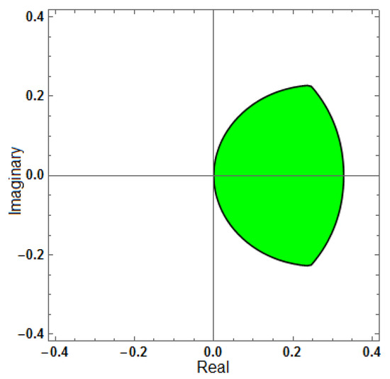
Figure 3. Region of stability for $E2$ (AF = 0), with $\eta =1$.

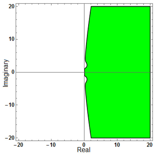
Figure 4. Region of stability for $E2$ (AF = 0), with $\eta =50$.

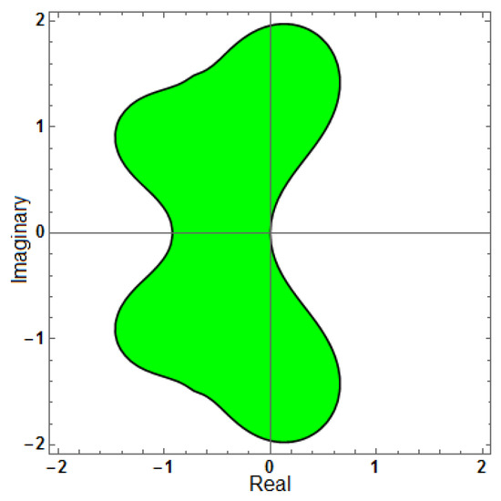
Figure 5. Region of stability for $E2$ (AF = 0), with $\eta =1000$.

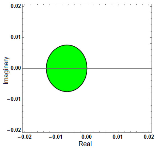
Figure 6. Region of stability for $E3$ (AF = 0, PhEr = 0), with $\eta =1$.

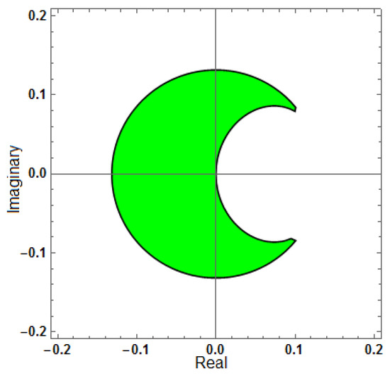
Figure 7. Region of stability for $E3$ (AF = 0, PhEr = 0), with $\eta =50$.

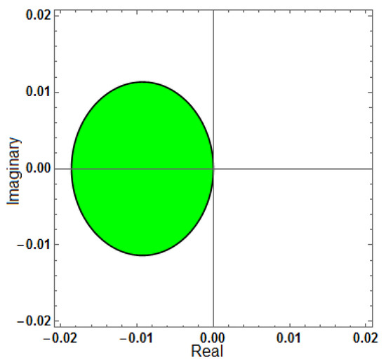
Figure 8. Region of stability for $E3$ (AF = 0, PhEr = 0), with $\eta =1000$.

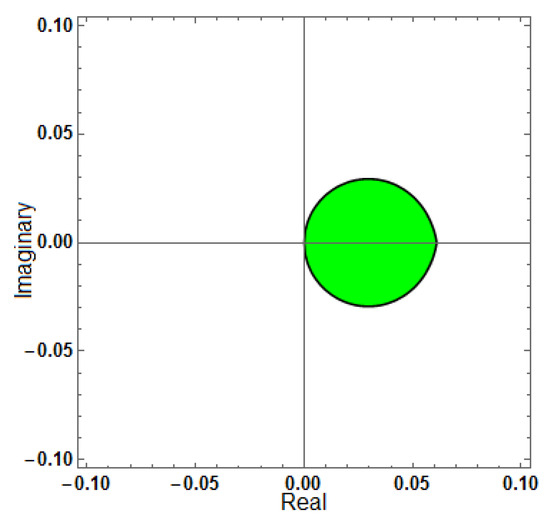
Figure 9. Region of stability for $E4$ (AF = 0, PhEr = 0, D[PhEr] = 0), with $\eta =1$.

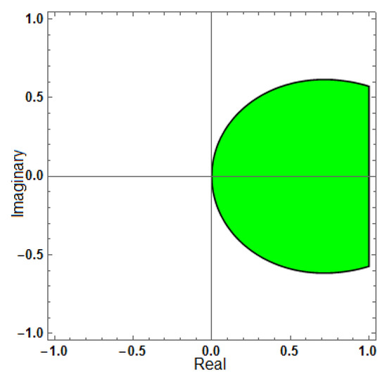
Figure 10. Region of stability for $E4$ (AF = 0, PhEr = 0, D[PhEr] = 0), with $\eta =50$.

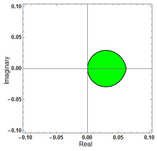
Figure 11. Region of stability for $E4$ (AF = 0, PhEr = 0, D[PhEr] = 0), with $\eta =1000$.

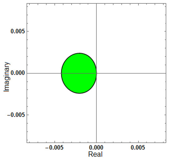
Figure 12. Region of stability for $E5$ (AF = 0, PhEr = 0, D[AF] = 0), with $\eta =1$.

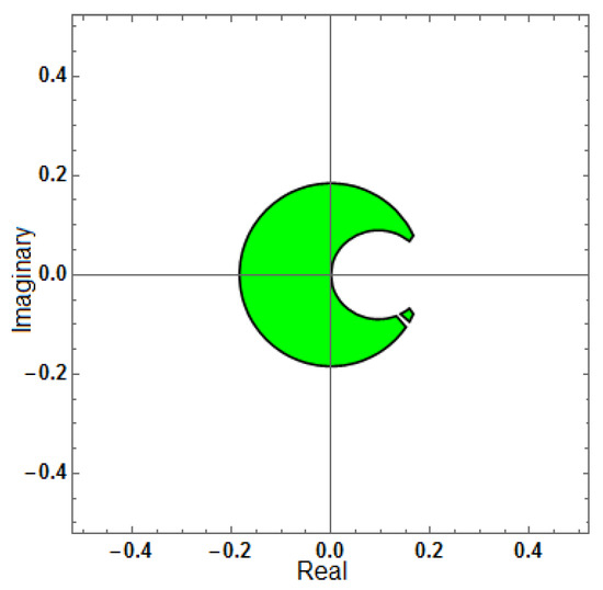
Figure 13. Region of stability for $E5$ (AF = 0, PhEr = 0, D[AF] = 0), with $\eta =50$.

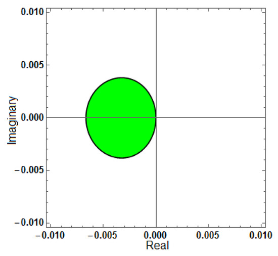
Figure 14. Region of stability for $E5$ (AF = 0, PhEr = 0, D[AF] = 0), with $\eta =1000$.

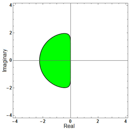
Figure 15. Region of stability for $Im2$ (AF = 0), with $\eta =1$.

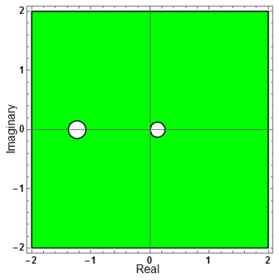
Figure 16. Region of stability for $Im2$ (AF = 0), with $\eta =50$.

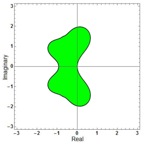
Figure 17. Region of stability for $Im2$ (AF = 0), with $\eta =1000$.

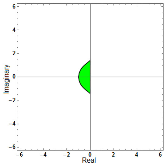
Figure 18. Region of stability for $Im3$ (AF = 0, PhEr = 0), with $\eta =1$.

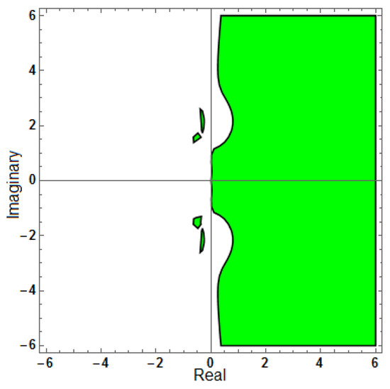
Figure 19. Region of stability for $Im3$ (AF = 0, PhEr = 0), with $\eta =50$.

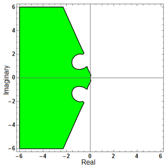
Figure 20. Region of stability for $Im3$ (AF = 0, PhEr = 0), with $\eta =1000$.

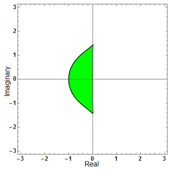
Figure 21. Region of stability for $Im4$ (AF = 0, PhEr = 0, D[PhEr] = 0), with $\eta =1$.

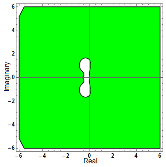
Figure 22. Region of stability for $Im4$ (AF = 0, PhEr = 0, D[PhEr] = 0), with $\eta =50$.

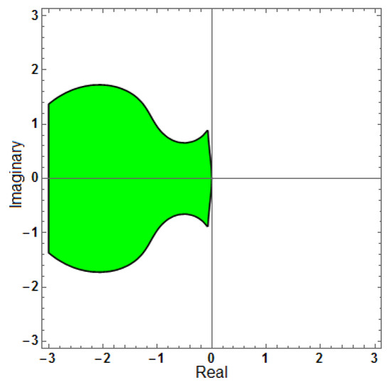
Figure 23. Region of stability for $Im4$ (AF = 0, PhEr = 0, D[PhEr] = 0), with $\eta =1000$.

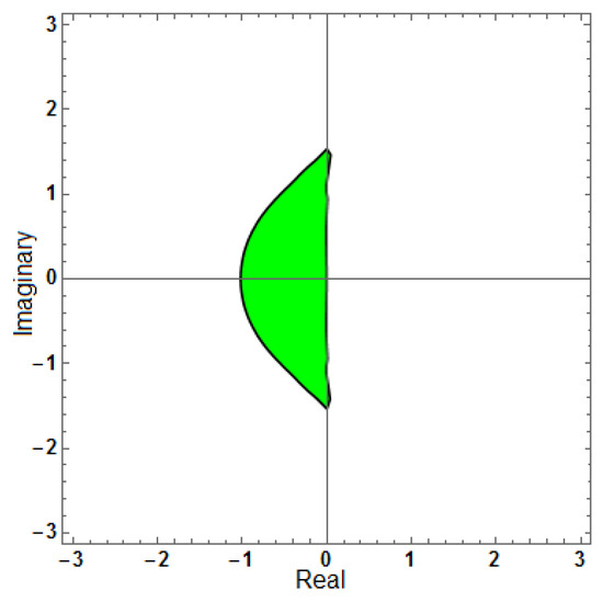
Figure 24. Region of stability for $Im5$ (AF = 0, PhEr = 0, D[AF] = 0), with $\eta =1$.

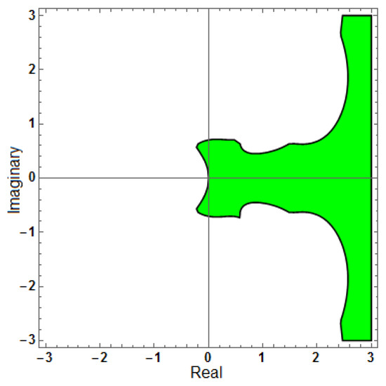
Figure 25. Region of stability for $Im5$ (AF = 0, PhEr = 0, D[AF] = 0), with $\eta =50$.

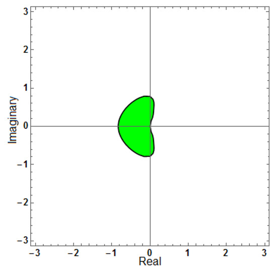
Figure 26. Region of stability for $Im5$ (AF = 0, PhEr = 0, D[AF] = 0), with $\eta =1000$.

4. Numerical Results

We investigated seven oscillatory ODE test problems and one PDE problem, the Telegraph equation. The accuracy associated with each case was determined using the following relation:

$$\mathrm{Errham}=-{\displaystyle \frac{\ln \left(\right|u\left(t_i\right)-u_i\left|\right)}{\ln \left(10\right)}}.$$

MATHEMATICA (Version number: 11.0.1.0) was used to solve the ODEs, while MATLAB R2017a was used to solve the PDE. An implicit optimized hybrid block method of atleast order five [24] and three ODE solvers from the Runge–Kutta family [25,26] have been compared: the fourth-order classical Runge–Kutta method (RK4), the fifth-order Cash–Karp method (RKCash), and the fifth-order Fehlberg method (RKFehl). For each problem, the first three steps were calculated using a high-order Runge–Kutta algorithm. Following this, the explicit block methods, as described earlier, served as the predictors, while the implicit block methods, also outlined above, were employed as the correctors.

The following numerical methods were employed to address the given problems:

• Hybrid: Optimized hybrid block method.
• RK4: Classical fourth-order Runge–Kutta method.
• RKCash: Fifth-order Cash–Karp method.
• RKFehl: Fifth-order Fehlberg method.
• M1: The method incorporates $Im1$ in the predictor–corrector mode, with $E1$ as the predictor.
• M2: The method utilizes $E2$ as the predictor and $Im2$ as the corrector.
• M3: The method applies $E3$ as the predictor and $Im3$ as the corrector.
• M4: This method uses the explicit method $E4$ as the predictor and $Im4$ as the corrector.
• M5: The method incorporates $Im5$ in the predictor–corrector mode, with $E5$ as the predictor.

Example 1. 

Consider the Stiefel and Bettis [27] problem, where the system of equations governing it is as follows:

$$\begin{array}{cc}\hfill u_1^{\prime \prime }\left(t\right)& =-u_1\left(t\right)+0.001\cos \left(t\right),u_1\left(0\right)=1,u_1^{\prime }\left(0\right)=0,\hfill \\ \hfill u_2^{\prime \prime }\left(t\right)& =-u_2\left(t\right)+0.001\sin \left(t\right),u_2\left(0\right)=0,u_2^{\prime }\left(0\right)=0.9995.\hfill \end{array}$$

(30)

The exact solution is

$$\begin{array}{cc}\hfill u_1\left(t\right)& =\cos \left(t\right)+0.0005t\sin \left(t\right),\hfill \\ \hfill u_2\left(t\right)& =\sin \left(t\right)-0.0005t\cos \left(t\right).\hfill \end{array}$$

(31)

The domain is defined to be $[0,10000]$. Numerical experiments were performed using the derived block methods $M1$ through $M5$ with $\omega =1$, and the results are illustrated in Figure 27. The following key insights have been drawn from the graphical comparison of these methods:

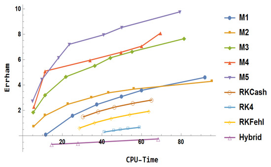
Figure 27. Error comparison for Example 1.

• The hybrid block method [24] (hybrid) underperformed, falling short of the efficiency and accuracy demonstrated by the other methods.
• The classical fourth-order Runge–Kutta method (RK4) exhibited the lowest accuracy among all methods considered.
• The fifth-order Runge–Kutta–Cash–Karp method (RKCash) demonstrated improved accuracy over both the Runge–Kutta–Fehlberg method (RKFehl) and RK4.
• The proposed implicit block methods $M1$–$M5$ consistently outperformed the traditional Runge–Kutta-based schemes (RK4, RKFehl, and RKCash) in terms of numerical accuracy and computational time.
• Method $M2$ showed a notable improvement over $M1$ in the early stages of computation but later $M1$ overtook the position.
• Method $M3$ further enhanced the accuracy compared to $M2$, indicating a clear progression in performance.
• Among all methods tested, $M5$ delivered the most accurate results, establishing its superiority in this comparative analysis.

Example 2. 

The inhomogeneous linear problem, examined by Franco et al. [28], is as follows:

$$\begin{array}{cc}\hfill u_1^{\prime \prime }\left(t\right)& =-{\displaystyle \frac{1}{2}}\left({\mu }^2+1\right)u_1\left(t\right)-{\displaystyle \frac{1}{2}}\left({\mu }^2-1\right)u_2\left(t\right),u_1\left(0\right)=1,u_1^{\prime }\left(0\right)=1,\hfill \\ \hfill u_2^{\prime \prime }\left(t\right)& =-{\displaystyle \frac{1}{2}}\left({\mu }^2-1\right)u_1\left(t\right)-{\displaystyle \frac{1}{2}}\left({\mu }^2+1\right)u_2\left(t\right),u_2\left(0\right)=-1,u_2^{\prime }\left(0\right)=-1.\hfill \end{array}$$

(32)

The exact solution is

$$\begin{array}{cc}\hfill u_1\left(t\right)& =\cos \left(t\right)+\sin \left(t\right),\hfill \\ \hfill u_2\left(t\right)& =-\cos \left(t\right)-\sin \left(t\right).\hfill \end{array}$$

(33)

Choosing $\mu ={10}^4$ and the solution domain as $[0,10,000]$, and the numerical solution of the system of equation was computed with $\omega =1$. The computational performance of the various methods, as illustrated in Figure 28, revealed the following key observations:

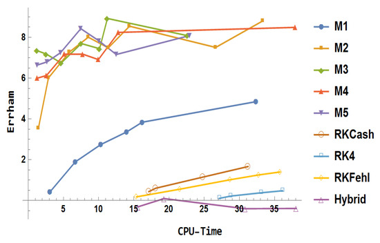
Figure 28. Error comparison for Example 2.

• The hybrid method was least efficient among the considered methods.
• Of the classical Runge–Kutta methods tested, RK4 attained the poorest accuracy, in contrast to RKFehl, which offered a moderate gain in precision.
• RKCash provided enhanced accuracy compared to RKFehl; however, the block method $M1$ significantly surpassed both in performance.
• Method $M2$ offered a marked improvement over $M1$, reflecting increased precision across the tested step sizes.
• For relatively large step sizes, $M3$ initially outperformed all other methods, followed by $M5$, $M4$, and $M2$, respectively.
• While $M5$ initially yielded better results than $M4$, the latter marginally overtook $M5$ as the step size decreased, suggesting improved efficiency in finer resolutions.
• Among all the methods considered, $M3$ consistently yielded the most accurate results on average.

Example 3. 

The problem presented by Franco and Palacios is defined as follows [29]:

$$\begin{array}{cc}\hfill u_1^{\prime \prime }\left(t\right)& =-u_1\left(t\right)+ϵ\cos \left(\vartheta t\right),u_1\left(0\right)=1,u_1^{\prime }\left(0\right)=0,\hfill \\ \hfill u_2^{\prime \prime }\left(t\right)& =-u_2\left(t\right)+ϵ\sin \left(\vartheta t\right),u_2\left(0\right)=0,u_2^{\prime }\left(0\right)=1,0\le t\le 10,000\hfill \end{array}$$

(34)

with the analytical solution given as

$$\begin{array}{cc}\hfill u_1\left(t\right)& ={\displaystyle \frac{1-ϵ-{\vartheta }^2}{1-{\vartheta }^2}}\cos \left(t\right)+{\displaystyle \frac{ϵ}{1-{\vartheta }^2}}\cos \left(\vartheta t\right),\hfill \\ \hfill u_2\left(t\right)& ={\displaystyle \frac{1-ϵ\vartheta -{\vartheta }^2}{1-{\vartheta }^2}}\sin \left(t\right)+{\displaystyle \frac{ϵ}{1-{\vartheta }^2}}\sin \left(\vartheta t\right),\hfill \end{array}$$

(35)

where $ϵ=0.001$ and $\vartheta =0.01$. To apply modified block methods, consider $\omega =max(1,|\vartheta \left|\right)$.

The essential points derived from Figure 29 are presented as follows:

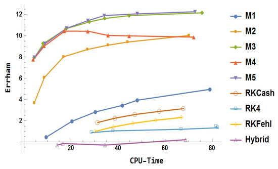
Figure 29. Error comparison for Example 3.

• Within the tested CPU time range, the hybrid block method (Hybrid) consistently fell below the performance benchmark set by the other methods.
• RKCash outperformed both RKFehl and RK4, with RK4 showing the least accuracy.
• The accuracy of the block method $M1$ surpassed that of the traditional Runge–Kutta approaches.
• Method $M2$ significantly outperformed $M1$ in terms of performance.
• A reduction in step size led to a consistent enhancement in the accuracy of $M2$.
• While $M4$ was more accurate than $M2$ for larger step sizes, both methods achieved the same level of accuracy as the step size reduced.
• $M5$ and $M3$ were nearly identical in terms of accuracy.
• Among all the methods, $M5$ and $M3$ were the most accurate.

The hybrid block method was excluded from further comparisons, as initial results demonstrated that it was computationally expensive and consistently less efficient than the Runge–Kutta methods and the proposed methods across the tested examples.

Example 4. 

Simos studied the nonlinear problem in [30] described as follows:

$$\begin{array}{cc}\hfill u_1^{\prime \prime }\left(t\right)& =-{\phi }^2{u}_1\left(t\right)+{\displaystyle \frac{2u_1\left(t\right)u_2\left(t\right)-\sin \left(2\phi t\right)}{{\left(u_1{\left(t\right)}^2+u_2{\left(t\right)}^2\right)}^{\frac{3}{2}}}},u_1\left(0\right)=1,u_1^{\prime }\left(0\right)=0,\hfill \\ \hfill u_2^{\prime \prime }\left(t\right)& =-{\phi }^2{u}_2\left(t\right)+{\displaystyle \frac{\left(u_1{\left(t\right)}^2-u_2{\left(t\right)}^2\right)-\cos \left(2\phi t\right)}{{\left(u_1{\left(t\right)}^2+u_2{\left(t\right)}^2\right)}^{\frac{3}{2}}}},u_2\left(0\right)=0,u_2^{\prime }\left(0\right)=\phi ,\hfill \end{array}$$

(36)

where $\phi =10$, $t\in [0,10000]$, and the exact solution is

$$\begin{array}{cc}\hfill u_1\left(t\right)& =\cos \left(\phi t\right),\hfill \\ \hfill u_2\left(t\right)& =\sin \left(\phi t\right).\hfill \end{array}$$

(37)

For $\omega =10$, the numerical results are presented in Figure 30. The following points summarize the key observations:

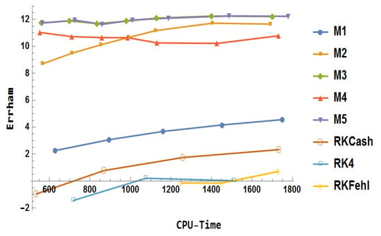
Figure 30. Error comparison for Example 4.

• The Runge–Kutta methods exhibited considerable computational overhead, yielding only marginal to negligible improvements in accuracy.
• Despite increased CPU time, RK4 failed to demonstrate a meaningful enhancement in performance.
• RKCash surpassed both RKFehl and RK4 in terms of overall efficiency and accuracy.
• The block method $M1$ consistently provided more precise results compared to the traditional Runge-Kutta approaches.
• Method $M2$ significantly outperformed $M1$ in terms of both computational efficiency and accuracy.
• Although $M2$ initially under-performed compared to $M4$ in terms of accuracy, it eventually surpassed $M4$ as the step size decreased, demonstrating superior performance.
• Methods $M3$ and $M5$ delivered nearly identical levels of accuracy.
• Among all methods, $M5$ and $M3$ exhibited the highest accuracy.

Example 5. 

The nonlinear first-order differential problem studied by Petzold [31] is defined as follows:

$$\begin{array}{cc}\hfill u_1^{\prime }\left(t\right)& =\lambda u_2\left(t\right),u_1\left(0\right)=1,\hfill \\ \hfill u_2^{\prime }\left(t\right)& =-\lambda u_1\left(t\right)+{\displaystyle \frac{\alpha }{\lambda }}\sin \left(\lambda t\right),u_2\left(0\right)=-{\displaystyle \frac{\alpha }{2{\lambda }^2}},\hfill \end{array}$$

(38)

with the analytical solution defined as

$$\begin{array}{cc}\hfill u_1\left(t\right)& =\left(1-{\displaystyle \frac{\alpha }{2\lambda }}t\right)\cos \left(\lambda t\right),\hfill \\ \hfill u_2\left(t\right)& =-\left(1-{\displaystyle \frac{\alpha }{2\lambda }}t\right)\sin \left(\lambda t\right)-{\displaystyle \frac{\alpha }{2{\lambda }^2}}\cos \left(\lambda t\right).\hfill \end{array}$$

(39)

The parameters are $\alpha =100,\lambda =1000,t\in [0,100]$. To employ modified block methods, $\omega =1000$ was chosen, and the results are plotted in Figure 31; the following lists the observations obtained:

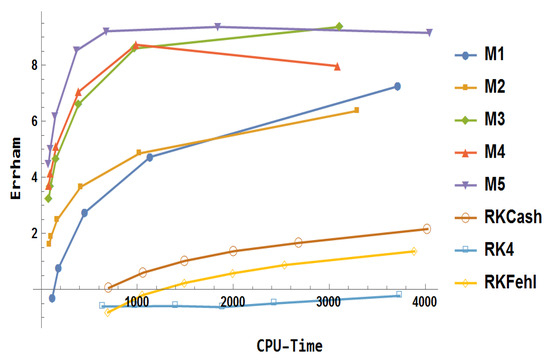
Figure 31. Error comparison for Example 5.

• RK4 failed to achieve an acceptable accuracy within the allocated CPU time.
• RKCash demonstrated superior overall performance compared to RKFehl.
• The block method $M1$ yielded more accurate results than RKCash, with the accuracy steadily improving as the CPU time increased.
• For large step sizes, $M1$ was the least accurate among the block methods, while $M5$ achieved the highest accuracy.
• Method $M2$ initially outperformed $M1$ in both computational efficiency and accuracy, although this trend reversed as the step size decreased.
• Methods $M3$ and $M4$ exhibited comparable performance in terms of both accuracy and efficiency up to a certain threshold, after which $M3$ surpassed $M4$.
• Method $M5$ emerge as the best performer overall.

Example 6. 

The two-body gravitational problem is considered as follows:

$$\begin{array}{cc}\hfill u_1^{\prime \prime }\left(t\right)& =-{\displaystyle \frac{u_1\left(t\right)}{{\left(u_1{\left(t\right)}^2+u_2{\left(t\right)}^2\right)}^{\frac{3}{2}}}},u_1\left(0\right)=1,u_1^{\prime }\left(0\right)=0,\hfill \\ \hfill u_2^{\prime \prime }\left(t\right)& =-{\displaystyle \frac{u_2\left(t\right)}{{\left(u_1{\left(t\right)}^2+u_2{\left(t\right)}^2\right)}^{\frac{3}{2}}}},u_2\left(0\right)=0,u_2^{\prime }\left(0\right)=1,\hfill \end{array}$$

(40)

and the exact solution is

$$\begin{array}{cc}\hfill u_1\left(t\right)& =\cos \left(t\right),\hfill \\ \hfill u_2\left(t\right)& =\sin \left(t\right).\hfill \end{array}$$

(41)

With the choice of $\omega =1$, the numerical results for $0\le t\le 10,000$ were obtained and are displayed in Figure 32. The key findings are summarized as follows:

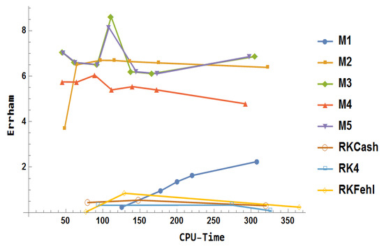
Figure 32. Error comparison for Example 6.

• The Runge–Kutta methods (RK4, RKCash, and RKFehl) exhibited marginal improvements, maintaining a steady level of performance without significant advancement.
• The block method $M1$ demonstrated superior accuracy compared to the traditional Runge–Kutta methods.
• Method $M2$ significantly outperformed $M1$ in terms of both accuracy and efficiency.
• As the step size decreased, $M2$ initially showed an increase in accuracy, which eventually stabilized.
• Initially, $M4$ surpassed $M1$ in performance, although it did not exceed the performance of $M2$.
• Method $M3$ was on par with $M5$ in terms of both accuracy and computational efficiency.
• The block method $M3$ provided more precise results compared to the others on average.

Example 7. 

Consider the perturbed two-body Kepler’s problem:

$$u_1^{\prime \prime }\left(t\right)=-{\displaystyle \frac{u_1\left(t\right)}{{\left(u_1{\left(t\right)}^2+u_2{\left(t\right)}^2\right)}^{3/2}}}-\mu \left(\mu +2\right){\displaystyle \frac{u_1\left(t\right)}{{\left(u_1{\left(t\right)}^2+u_2{\left(t\right)}^2\right)}^{5/2}}},0\le t\le 10000,$$

$$u_1\left(0\right)=1,u_1^{\prime }\left(0\right)=0,$$

$$u_2^{\prime \prime }\left(t\right)=-{\displaystyle \frac{u_2\left(t\right)}{{\left(u_1{\left(t\right)}^2+u_2{\left(t\right)}^2\right)}^{3/2}}}-\mu \left(\mu +2\right){\displaystyle \frac{u_2\left(t\right)}{{\left(u_1{\left(t\right)}^2+u_2{\left(t\right)}^2\right)}^{5/2}}},$$

$$u_2\left(0\right)=0,u_2^{\prime }\left(0\right)=1+\mu ,$$

where its analytical solution is

$$u_1\left(t\right)=\cos (t+\mu t),u_2\left(t\right)=\sin (t+\mu t).$$

The value $\omega =\sqrt{1+\mu \left(\mu +2\right)},\mu =0.1$ was considered. From Figure 33, the following observations can be made:

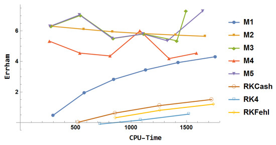
Figure 33. Error comparison for Example 7.

• The Runge–Kutta methods (RK4, RKFehl, and RKCash) showed only marginal improvements in both accuracy and efficiency, with RK4 performing the least effectively.
• The block method $M1$ surpassed all Runge–Kutta methods in terms of accuracy.
• Method $M4$ delivered superior performance compared to $M1$.
• Method $M3$ maintained a consistent level of accuracy, even when using large step sizes, with its performance remaining relatively stable regardless of the chosen step size.
• The performance of $M3$ was equivalent to that of $M5$.
• Method $M3$ outperformed $M4$ in terms of both accuracy and computational efficiency.
• On average, $M3$ and $M5$ outperformed all other methods in terms of both accuracy and efficiency.

Example 8. 

Consider the hyperbolic telegraph equation

$$u_{tt}(z,t)+2a{u}_t(z,t)+b^{2}u(z,t)=u_{zz}(z,t)+f(z,t),0\le z\le 1,t\ge 0.$$

The initial and boundary conditions are given by

$$u(z,0)=\sin \left(z\right),u_t(z,0)=0,0\le z\le 1;$$

$$u(0,t)=0,u(1,t)=\cos \left(t\right)\sin \left(1\right),t\ge 0.$$

The parameters are chosen as $a=6$, $b=2$, and

$$f(z,t)=-2a\sin \left(t\right)\sin \left(z\right)+b^2\cos \left(t\right)\sin \left(z\right).$$

The analytic solution is

$$u(z,t)=\cos \left(t\right)\sin \left(z\right).$$

For the block methods, the parameter $\omega =1$ was selected. These methods were implemented using the algorithm outlined in [19]. Using [19], block methods were combined with the differential quadrature method, utilizing unified splines for the spatial variable. The following key observations can be made:

• The error analysis in Figure 34 for $t=1$ shows that $M3$ provided superior accuracy relative to $M1$.
  

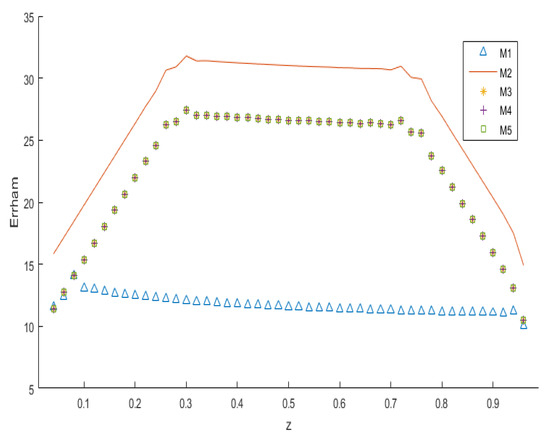  Figure 34. Error comparison for Example 8.
• Methods $M3$, $M4$, and $M5$ exhibited virtually identical accuracy across the spatial grid.
• Method $M3$ significantly outperformed $M1$ in terms of accuracy.
• The CPU times for $t=1$ differed among the methods: $M1$ took 1.810412 s, $M2$ required 0.021124 s, $M3$ completed in 0.020640 s, $M4$ took 0.021212 s, and $M5$ required 0.017187 s.
• In terms of overall performance, $M2$ outperformed the other methods.

The performance of frequency-dependent approaches, including the newly proposed method, largely hinges on the appropriate selection of the parameter $\omega$. Often, this parameter can be directly inferred from the characteristics of the specific problem being addressed. In cases where determining $\omega$ is less straightforward, several strategies for its estimation have been developed and discussed in existing studies [2,4].

5. Conclusions

In summary, the block methods demonstrated a marked advantage over the traditional Runge–Kutta methods and optimized hybrid block method, with $M1$ notably outperforming RK4, RKFehl, and RKCash. As the study advanced to the implementation of the modified block methods $M2$, $M3$, $M4$, and $M5$, the results demonstrated a consistent enhancement in both accuracy and computational efficiency. Among these, $M2$ and $M4$ exhibited a competitive performance, with no clear winner emerging, as the effectiveness of numerical methods is highly contingent upon the specific characteristics of the problem at hand. However, $M5$ consistently proved to be the most robust method, delivering superior results across a range of problem types. For partial differential equations (PDEs), method $M2$ particularly excelled, showcasing its potential for complex applications. This study not only provides a thorough evaluation of the methods’ performance but also underscores the broad applicability and potential of modified implicit block methods in diverse numerical scenarios. These findings expand the scope for their use in more complex and varied computational problems, offering promising avenues for future research and development.

References

- Landau, L.D.; Lifshitz, E.M. Quantum Mechanics: Non-Relativistic Theory; Pergamon Press: Oxford, UK, 1965. [Google Scholar]
- Ixaru, L.G.; Berghe, G.V.; DeMeyer, H. Frequency evaluation in exponential fitting multistep algorithms for ODEs. J. Comput. Appl. Math. 2002, 140, 423–434. [Google Scholar] [CrossRef]
- Lee, K.C.; Senu, N.; Ahmadian, A.; Ibrahim, S.N.I. High-order exponentially fitted and trigonometrically fitted explicit two-derivative Runge–Kutta-type methods for solving third-order oscillatory problems. Math. Sci. 2022, 16, 281–297. [Google Scholar] [CrossRef]
- Ramos, H.; Vigo-Aguiar, J. On the frequency choice in trigonometrically fitted methods. Appl. Math. Lett. 2010, 23, 1378–1381. [Google Scholar] [CrossRef]
- Raptis, A.; Allison, A. Exponential-fitting methods for the numerical solution of the schrodinger equation. Comput. Phys. Commun. 1978, 14, 1–5. [Google Scholar] [CrossRef]
- Senu, N.; Lee, K.; WanIsmail, W.; Ahmadian, A.; Ibrahim, S.; Laham, M. Improved Runge-Kutta method with trigonometrically-fitting technique for solving oscillatory problem. Malays. J. Math. Sci. 2021, 15, 253–266. [Google Scholar]
- Simos, T.E. A new methodology for the development of efficient multistep methods for first-order IVPs with oscillating solutions. Mathematics 2024, 12, 504. [Google Scholar] [CrossRef]
- Thomas, R.; Simos, T. A family of hybrid exponentially fitted predictor-corrector methods for the numerical integration of the radial Schrödinger equation. J. Comput. Appl. Math. 1997, 87, 215–226. [Google Scholar] [CrossRef][Green Version]
- Van de Vyver, H. A symplectic exponentially fitted modified Runge–Kutta–Nyström method for the numerical integration of orbital problems. New Astron. 2005, 10, 261–269. [Google Scholar] [CrossRef]
- Zhai, W.; Fu, S.; Zhou, T.; Xiu, C. Exponentially-fitted and trigonometrically-fitted implicit RKN methods for solving y”= f (t, y). J. Appl. Math. Comput. 2022, 68, 1449–1466. [Google Scholar] [CrossRef]
- Butcher, J.C. The Numerical Analysis of Ordinary Differential Equations: Runge-Kutta and General Linear Methods; Wiley-Interscience: Hoboken, NJ, USA, 1987. [Google Scholar]
- Hairer, E.; Wanner, G. Convergence for nonlinear problems. Solving Ordinary Differential Equations II: Stiff and Differential-Algebraic Problems; Springer: Berlin/Heidelberg, Germany, 1996; pp. 339–355. [Google Scholar]
- Birta, A.-B. Parallel block predictor-corrector methods for ODE’s. IEEE Trans. Comput. 1987, C-36, 299–311. [Google Scholar] [CrossRef]
- Chu, M.T.; Hamilton, H. Parallel solution of ODE’s by multiblock methods. SIAM J. Sci. Stat. Comput. 1987, 8, 342–353. [Google Scholar] [CrossRef]
- Shampine, L.F.; Watts, H. Block implicit one-step methods. Math. Comput. 1969, 23, 731–740. [Google Scholar] [CrossRef]
- Tam, H.W. Parallel Methods for the Numerical Solution of Ordinary Differential Equations; University of Illinois at Urbana-Champaign: Chicago, IL, USA, 1989. [Google Scholar]
- Gragg, W.B.; Stetter, H.J. Generalized multistep Predictor-Corrector methods. J. ACM (JACM) 1964, 11, 188–209. [Google Scholar] [CrossRef]
- Milne, W.E. Numerical solution of differential equations. Bull. Am. Math. Soc. 1953, 59, 577–579. [Google Scholar] [CrossRef][Green Version]
- Kaur, A.; Kanwar, V.; Ramos, H. A coupled scheme based on uniform algebraic trigonometric tension B-spline and a hybrid block method for Camassa-Holm and Degasperis-Procesi equations. Comput. Appl. Math. 2024, 43, 16. [Google Scholar] [CrossRef]
- Fatunla, S.O. Numerical Methods for Initial Value Problems in Ordinary Differential Equations; Academic Press: Cambridge, MA, USA, 1988. [Google Scholar]
- Fatunla, S.O. Block methods for second order ODEs. Int. J. Comput. Math. 1991, 41, 55–63. [Google Scholar] [CrossRef]
- Lambert, J.D. Computational Methods in Ordinary Differential Equations; Wiley: Hoboken, NJ, USA, 1973. [Google Scholar]
- Chollom, J.; Ndam, J.; Kumleng, G. On some properties of the block linear multi-step methods. Sci. World J. 2007, 2, 11–17. [Google Scholar] [CrossRef]
- Singh, G.; Garg, A.; Kanwar, V.; Ramos, H. An efficient optimized adaptive step-size hybrid block method for integrating differential systems. Appl. Math. Comput. 2019, 362, 124567. [Google Scholar] [CrossRef]
- Cash, J.R.; Karp, A.H. A variable order Runge-Kutta method for initial value problems with rapidly varying right-hand sides. ACM Trans. Math. Softw. 1990, 16, 201–222. [Google Scholar] [CrossRef]
- Fehlberg, E. Classical Fifth-, Sixth-, Seventh-, and Eighth-Order Runge-Kutta Formulas with Stepsize Control; National Aeronautics and Space Administration: Washington, DC, USA, 1968.
- Stiefel, E.; Bettis, D. Stabilization of Cowell’s method. Numer. Math. 1969, 13, 154–175. [Google Scholar] [CrossRef]
- Franco, J.; Gómez, I.; Rández, L. Four-stage symplectic and P-stable SDIRKN methods with dispersion of high order. Numer. Algorithms 2001, 26, 347–363. [Google Scholar] [CrossRef]
- Franco, J.; Palacios, M. High-order P-stable multistep methods. J. Comput. Appl. Math. 1990, 30, 1–10. [Google Scholar] [CrossRef]
- Simos, T. New open modified Newton Cotes type formulae as multilayer symplectic integrators. Appl. Math. Model. 2013, 37, 1983–1991. [Google Scholar] [CrossRef]
- Petzold, L.R. An efficient numerical method for highly oscillatory ordinary differential equations. SIAM J. Numer. Anal. 1981, 18, 455–479. [Google Scholar] [CrossRef]
Disclaimer/Publisher’s Note: The statements, opinions and data contained in all publications are solely those of the individual author(s) and contributor(s) and not of MDPI and/or the editor(s). MDPI and/or the editor(s) disclaim responsibility for any injury to people or property resulting from any ideas, methods, instructions or products referred to in the content. |
© 2025 by the authors. Licensee MDPI, Basel, Switzerland. This article is an open access article distributed under the terms and conditions of the Creative Commons Attribution (CC BY) license (https://creativecommons.org/licenses/by/4.0/).