Optimal Control and Tumour Elimination by Maximisation of Patient Life Expectancy

Abstract

We propose a life-expectancy pay-off function (LEP) for determining optimal cancer treatment within a control theory framework. The LEP averages life expectancy over all future outcomes, outcomes that are determined by key events during therapy such as tumour elimination (cure) and patient death (including treatment related mortality). We analyse this optimisation problem for tumours treated with chemotherapy using tumour growth models based on ordinary differential equations. To incorporate tumour elimination we draw on branching processes to compute the probability distribution of tumour population extinction. To demonstrate the approach, we apply the LEP framework to simplified one-compartment models of tumour growth that include three possible outcomes: cure, relapse, or death during treatment. Using Pontryagin’s maximum principle (PMP) we show that the best treatment strategies fall into three categories: (i) continuous treatment at the maximum tolerated dose (MTD), (ii) no treatment, or (iii) treat-and-stop therapy, where the drug is given at the MTD and then halted before the treatment (time) horizon. Optimal treatment strategies are independent of the time horizon unless the time horizon is too short to accommodate the most effective (treat-and-stop) therapy. For sufficiently long horizons, the optimal solution is either no treatment (when treatment yields no benefit) or treat-and-stop. Patients, thus, split into an untreatable class and a treatable class, with patient demographics, tumour size, tumour response, and drug toxicity determining whether a patient benefits from treatment. The LEP is in principle parametrisable from data, requiring estimation of the rates of each event and the associated life expectancy under that event. This makes the approach suitable for personalising cancer therapy based on tumour characteristics and patient-specific risk profiles.

1. Introduction

Optimal therapy strategies for cancer patients can be formulated as a control theory problem, [1,2,3,4,5,6,7,8], to determine the optimal dose and schedule of chemotherapy, or optimal combination and timing of treatments to control tumour size and achieve the best outcome. Available treatments, the controls, include chemotherapy, resection surgery (tumour removal), radiotherapy, and transplant (blood cancers). For chemotherapy, the optimal concentration of the drug(s) at each point in time must be determined. Control theory formulations require specification of a model of cancer growth under therapy (incorporating the mechanism of action and efficacy of a drug), and a mathematical function (the objective) to be optimised, potentially a function of the tumour state, patient health and therapy strength/impact, both throughout the treatment interval and at the end of therapy. This control problem can be formulated in a deterministic framework (ODEs, PDEs), allowing Pontryagin’s Maximum principle (PMP) to be used [9], or as a stochastic control problem. Deterministic control theory frameworks have substantial advantages, being both analytically and numerically more tractable. There is also a far more extensive literature on deterministic models of cancer growth. Tumour growth is complex and notoriously difficult to model and parametrise, although with recent technological innovations there are an increasing number of validated chemotherapy cancer models of varying complexity [10,11,12,13].

The optimisation criterion is a fundamental part of the optimisation problem and has a significant impact on the nature of the optimal solutions [5,14]. Optimisation criteria are needed since there are competing objectives for therapy—the control of the tumour (for instance, minimising tumour size at the end of therapy) and minimising the risk of therapy to the patient. A chemotherapy control problem is typically set up as follows: treatment occurs up to a time T (the time horizon) using a time dependent control $u\left(t\right),t\in [0,T]$ that is assumed bounded, $u\left(t\right)\in [0,u_{max}]$, where $u_{max}$ is, for instance, the maximum tolerated dose (MTD) of a chemotherapy drug. The optimal dosing protocol, $u\left(t\right)$, is then determined by optimising an objective function, for instance,

$$J[N,u]=rN\left(T\right)+{\int }_0^{T}u{\left(t\right)}^{\nu }dt,$$

(1)

comprising a terminal cost proportional to the tumour size $N\left(T\right)$ at the end of the treatment horizon T and a running cost that accounts for factors such as drug toxicity during treatment. Here $N\left(t\right)$ is the tumour size at time t. The positive constant r determines the relative weight of the two competing objectives, specifically balancing the need to minimise the tumour burden at the end of treatment and reducing toxicity to the patient. The $L^2$ norm, with $\nu =2$, is more amenable to mathematical analysis, whilst the $L^1$ norm is more biologically justifiable. A variety of other objectives have been used, but all typically have the same qualitative form and incorporate a weight to balance the competing objectives.

Such objectives do not have any medical justification or foundation, only capturing qualitatively the competing demands of treatment which limits their application to decision making in the clinic. Further, this formulation assumes a continuum of benefits and costs, whilst cancer therapy is punctuated by key events that substantially affect outcome and post-treatment prognosis. In particular, in these deterministic models the cancer regrows in the absence of therapy and, therefore, tumour elimination (cure) is ignored; these optimisation problems in fact restrict focus to the period $[0,T]$ and ignore outcomes beyond T. There are also other events of key importance to patient prognosis, for instance treatment can have severe adverse effects (SAEs) on patient health, [15], drug resistant (mutant) cells can appear [16], and the cancer may undergo metastasis, i.e., spreading and colonising to other tissues and sites in the body [17]. SAEs can result in cessation of treatment or patient death in extreme cases, drug resistance limits possible therapies [18], whilst the prognosis for metastatic cancers is poor [19].

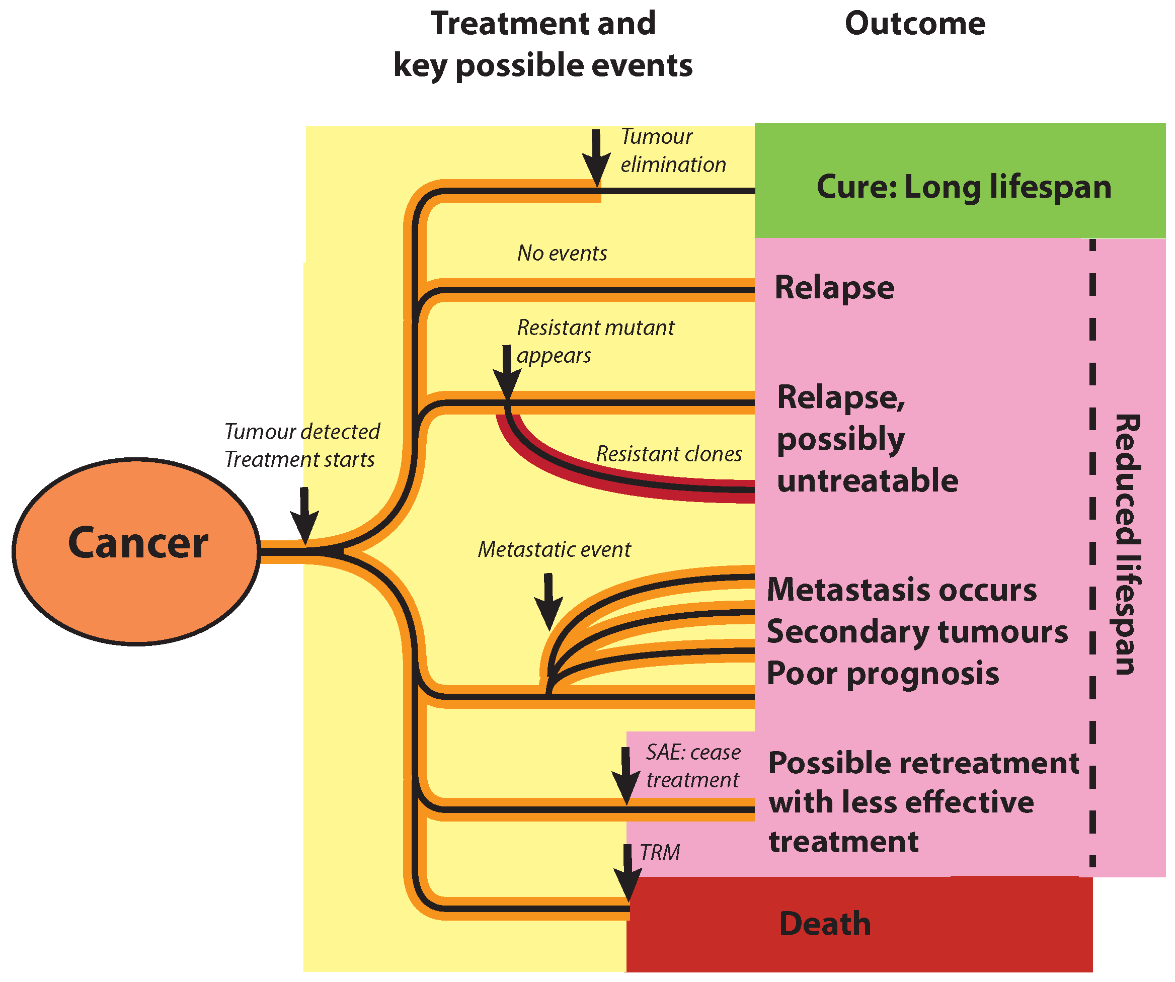
Here we propose a new objective function that incorporates these key events, Figure 1, including complete remission (cure), failure to eliminate the tumour, SAE, metastasis, and generation of mutants (both treatable and untreatable) during treatment. It utilises the rate of these events, so that at the end of therapy we can calculate the probability of each event having occurred, events that impact patient outcome and future prognosis. Thus, our formulation implicitly incorporates considerations post-treatment. To formulate an objective we observe that these events impact patient lifespan, thereby giving a common measure to quantify the impact of these events. We therefore propose to maximise the patient’s expected lifespan, averaged over possible events. This idea was proposed and explored in an earlier work using a simple approximation to the tumour elimination probability [20]. Consider a patient with a tumour of size $N\left(t\right)$, that is treated over a (horizon) time T, treatment administered as a control $u\left(t\right)$, $t\in [0,T]$ that directly affects the tumour’s growth dynamic. For instance, this could model a chemotherapy drug administered at concentration $u\left(t\right)$. The outcome of therapy, and the expected lifespan of the patient, is determined by a set of countable events indexed by $j=1,\dots ,n$. We assume that events occur at time t with rate ${\mu }_j(N,u;t)$, which depends on the tumour size $N\left(t\right)$, the control $u\left(t\right)$, and possibly explicitly on time. Events, thus, follow a Poisson process; the probability of event j occurring by time t is $p_j[N,u;t]=1-exp\left(-{\int }_0^t{\mu }_j(N,u;s)ds\right)$, which is a function of the tumour history and control schedule. The rate of tumour elimination is dependent on fluctuations in the number of tumour cells; thus, we draw on branching processes to determine the probability of tumour elimination. The occurrence of an event may affect the rates of other events, thus, multiple event sequences need to be considered. Let k index all possible (allowable) sequences of events or futures (there are a maximum of $n!$, assuming an event happens only once); event combinations/futures are distributed as a multiple event Poisson process, giving the probability $p_k[N,u;t]$ of event combination k occurring by time t. Under event combination k let the expected lifespan be $L_k$. Therefore, under control schedule u the expected lifetime, or payoff, is,

$$J_0[N,u;T]=\sum _k{p}_k[N,u;T]L_k.$$

(2)

More generally this could also incorporate an integration over futures parametrised by a continuum. The optimal control schedule $u^{\ast }\left(t\right),t\in [0,T]$, is then the schedule that maximises this expected lifetime, i.e., $u^{\ast }$ maximises (2) subject to the growth dynamics. The outcome at the horizon time can then be classified into which events occurred, event k occurring with probability $p_k[N,u;T]$. This objective has to satisfy a consistency constraint; if the optimal control is zero at the horizon time, $u^{\ast }\left(t\right)=0,t\in [T-ϵ,T],ϵ>0$, then the expected lifespan is invariant to a reduction of T as the therapy is unchanged—the expected lifetime only changes by application of the control. In particular, if $u^{\ast }$ is zero at T the probability of tumour elimination must also be invariant to changes in T.

We develop this therapy optimisation framework within a deterministic context, which has substantial advantages over stochastic models in terms of model flexibility (with a range of nonlinear and multi-compartment ODE tumour growth models in the literature [1,2,3,4,5,6,7,8], and powerful optimisation tools such as PMP [1,21]. The competing objectives of therapy, tumour control/elimination, and minimising treatment related harm to the patient, are incorporated as impacts on the expected lifespan. We develop two payoff functionals. Firstly, we formulate a model where the drug impacts patient quality of life, giving the discounted expected lifespan payoff (DLP), Section 2, similar to the objective (1). Secondly, we propose a model where the negative effects of therapy are incorporated as SAEs. Specifically, we model treatment related mortality (TRM) events giving the severe adverse effects payoff (SAP), Section 5. For both of these payoffs, the optimal solutions separate patients into an untreatable class and a treatable class based on patient demographics, tumour size at detection, and the patient’s susceptibility to the drug’s side effects.

Maximising patient lifespan is not a new concept; it has been used as an optimisation criteria in a control theory analysis of patients with lethal/incurable forms of cancer. Originally analysed in [22] for the cases where resistant mutant cells pre-exist, it has been extended with a number of analyses since, including [23] which maximises the time to remain within a safe (or viability) region. Typically, these models incorporate tumour and normal cells, the safe region being defined by thresholds on both cell types. Maximising life expectancy is also similar to maximisation of overall survival (OS) used in sequentially adaptive medical decision-making where treatment is considered in multiple stages (drawn from a set of defined therapies), also known as dynamic treatment regime models, [24]; for instance, induction therapy and salvage therapy if induction fails. These problems are formulated in the Markov decision making framework. Such methods have been used to optimise sequential drug use, for instance, for acute myeloid leukaemia (AML) [25]. These models are based on probabilistic outcomes of events to determine optimal strategies and do not include explicit tumour dynamics, and are, thus, distinct from our approach.

This paper is organised as follows. In Section 2, we formulate the DLP. In Section 3, the functional form of the control probability of tumour lineage elimination is derived. In Section 4, PMP is applied to determine the optimal solutions of the DLP, subject to non-linear tumour evolution models. In Section 4, optimal drug administration strategies of the DLP subject to a logistic tumour evolution model are presented. In Section 5 the SAP is introduced and optimal drug administration strategies are determined. In Section 6, we discuss our framework and its limitations, and provide future directions.

2. The Discounted Life Expectancy Pay-Off (DLP)

The cost of treatment to the patient needs to be incorporated into the objective $J_0$, (2); for instance, the impact of drug toxicity on the patient. The simplest toxicity model is to deduct from the payoff (2) a cost of treatment measured in days, $R[N,u;T]=\gamma {\int }_0^{T}u\left(t\right)dt$, assuming toxicity is linear in the drug concentration. This simple model of toxicity is often used in control theory analysis of tumours [1,9]. In the lifetime context, this can be interpreted as a poor quality of life during treatment, e.g., nausea caused by the drug. Duration of treatment is in fact a significant covariate of a patient’s quality of life [26]. Assuming expected lifetimes are linear in age, the expected lifetime of outcome k at time T in the future is $L_k\left(T\right)=L_k-T$. We then obtain the payoff,

$$J[N,u;T]=\sum _k{p}_k[N,u;T]L_k\left(T\right)+T-R[N,u;T],$$

(3)

where both the payoff and the cost $R[N,u;T]$ are quantified in days. Then, $T-R[N,u;T]$ is a measure of the quality of life during treatment, effectively the days during treatment ‘worth living’, which can possibly be determined from quality-of-life (QoL) aggregate measures derived from patient-reported outcomes [26]. If drug concentration is rescaled to the maximum tolerated dose (MTD), i.e., $u\left(t\right)\in [0,1]$, then this interpretation imposes $\gamma \le 1$, and is expected to be of order 1.

Consider two possible outcomes—cure (tumour elimination), and a failure to eliminate the tumour, so the patient will subsequently relapse. Define $p[N,u;T]$ as the probability that the treatment achieves tumour elimination within time T, a functional of the tumour history. Define the expected lifetimes post-treatment, $L_e\left(T\right),L_n\left(T\right)$ for tumour elimination and no elimination. The expected lifetime $L_n\left(T\right)$ could be parametrised by tumour size, $L_n(T,N\left(T\right))$ if dependence is known. The pay-off function then reads,

$$J[N,u;T]=L_e\left(T\right)p[N,u;T]+L_n\left(T\right)(1-p[N,u;T])+T-{\int }_0^T\gamma u\left(t\right)dt$$

assuming a linear drug toxicity effect. Rearranging, we get

$$\begin{array}{ccc}\hfill J[N,u;T]& =& (L_e\left(T\right)-L_n\left(T\right))p[N,u;T]+L_n\left(T\right)+T-{\int }_0^T\gamma u\left(t\right)dt\hfill \\ & =& (L_e-L_n)p[N,u;T]+L_n-{\int }_0^T\gamma u\left(t\right)dt,\hfill \end{array}$$

(4)

the second line following under the assumption of linearity of expected lifetime estimates over the period T. Here we are assuming that the treatment horizon is shorter than the lifetime $L_n$, otherwise, $L_n\left(T\right)$ is negative and death during treatment would need to be separated out as a possible outcome, see Section 5.

3. Computation of the Tumour Elimination Probability

Here, we draw on branching processes to determine the probability of tumour elimination for exponentially growing tumours, and then generalise to non-linear dynamics. For the case of a tumour capacity, which is typical for non-linear dynamics, the probability of die-out is 1 as $t\to \infty$, i.e., given sufficient time there will be a sufficiently large fluctuation that will eliminate the population of tumour cells. To handle this, and determine the treatment related tumour extinction, we utilise the conditional probability of tumour elimination by therapy.

3.1. Probability of Tumour Elimination: Exponential Growth

To compute the probability of tumour elimination we consider a branching process (BP) with $N\left(t\right)$ independent cells and time dependent birth and death rates, $a\left(t\right),b\left(t\right)$, reflecting the effect of treatment through time; in the absence of a drug, we assume the birth and death rates are constant, $a_0$, $b_0$, respectively, with $a_0>b_0$. The tumour control probability (TCP) is the probability of tumour cell elimination, $P\left(N\right(T)=0|N\left(0\right)=M)$, that can be solved using the method of characteristics, see Appendix A [27]. The TCP is given by

$$\mathrm{TCP}(t)={\left(1-{\left(\mathsf{\Lambda }\left(t\right)+{\int }_0^{t}a\left(t^{\prime }\right)\mathsf{\Lambda }\left(t^{\prime }\right)d{t}^{\prime }\right)}^{-1}\right)}^M$$

(5)

where $\mathsf{\Lambda }\left(t\right)$ satisfies the ODE,

$${\displaystyle \frac{\mathrm{d}\mathsf{\Lambda }}{\mathrm{d}t}}=\left(b\left(t\right)-a\left(t\right)\right)\mathsf{\Lambda },\mathrm{with}\mathrm{solution}\mathsf{\Lambda }\left(t\right)=exp{\int }_0^t\left(b\left(t^{\prime }\right)-a\left(t^{\prime }\right)\right)d{t}^{\prime },$$

(6)

satisfying $\mathsf{\Lambda }\left(0\right)=1$.

The mean tumour size, $N\left(t\right)=\mathbf{E}\left[Z\right(t\left)\right]$, satisfies the ODE,

$${\displaystyle \frac{\mathrm{d}N}{\mathrm{d}t}}=\left(a\left(t\right)-b\left(t\right)\right)N,\mathrm{with}N\left(0\right)=M,$$

(7)

i.e., tumour growth is linear in tumour size, and tumour size is exponential for constant u. We have ${\displaystyle \frac{\mathrm{d}}{\mathrm{d}t}}\left(N\mathsf{\Lambda }\right)=0$, giving $\mathsf{\Lambda }\left(t\right)=N\left(0\right)/N\left(t\right)$. Thus, we have the TCP expression,

$$\mathrm{TCP}(t)={\left(1-{\left(N\left(0\right)G\left(t\right)\right)}^{-1}\right)}^{N\left(0\right)}\mathrm{with}G\left(t\right)={\displaystyle \frac{\mathsf{\Lambda }\left(t\right)}{N\left(0\right)}}+{\int }_0^{t}a\left(t^{\prime }\right){\displaystyle \frac{\mathsf{\Lambda }\left(t^{\prime }\right)}{N\left(0\right)}}d{t}^{\prime }={\displaystyle \frac{1}{N\left(t\right)}}+{\int }_0^t{\displaystyle \frac{a\left(t^{\prime }\right)}{N\left(t^{\prime }\right)}}d{t}^{\prime }.$$

(8)

For large $N\left(0\right)$, and assuming $N\left(t\right)<N\left(0\right)$ throughout the horizon, this is well approximated by

$$\mathrm{TCP}\left(t\right)=exp\left(-G{\left(t\right)}^{-1}\right),$$

(9)

which is valid provided $N\left(0\right)$ is sufficiently large (always expected to be the case). The condition $N\left(t\right)<N\left(0\right)$ can in fact be ignored, since the kernel in $G\left(t\right)$ is negligible when this does not hold. Therefore, we use this approximation for all histories. This approximation simplifies the LEP and, thus, the following optimisation analysis; however, the LEP can be formulated without using this approximation, i.e., using the TCP in Equation (8), giving a more complex expression for the objective. This would allow the LEP framework to be used with a small initial tumour size. Observe that explicit dependence on $N\left(0\right)$ has cancelled, so the initial condition is irrelevant, provided it is large enough. Observe that at $t=0$, this expression is not zero, although its value, $e^{-N_0}$, is exponentially small in $N_0$.

We note that for the BP,

$${\displaystyle \frac{\mathrm{d}G}{\mathrm{d}t}}=b\left(t\right){\displaystyle \frac{\mathsf{\Lambda }\left(t\right)}{N\left(0\right)}}\ge 0$$

(10)

since $b\left(t\right)$, the death rate, is non-negative. Both ${(1-x^{-1})}^M$ and $e^{-x^{-1}}$ are monotonically increasing with x and, thus, the TCP does not decrease in time, as expected, with die-out event probabilities accumulating over time. Thus, even if the deterministic solution for the mean tumour size $N\left(t\right)$ increases, (7), for instance, after cessation of treatment, the die-out probability from any interval where die-out was likely is retained in the TCP. We also note that post-treatment, when $b\left(t\right)=b_0$ (the drug free death rate), $G\left(t\right)$ continues to increase if $b_0>0$. This is because in the branching process lineages may die out by chance. Thus, treatment up to T may not eliminate the tumour by T, but lead to elimination post treatment, e.g., if the tumour burden at $t=T$ is only a few cells, these may die out. This die-out after the treatment horizon needs to be incorporated, as tumour elimination during or after treatment gives the same expected lifetime. Thus, we want to compute the probability of eliminating the tumour at $t=\infty$ by treatment within the interval of time $[0,T]$; specifically, only lineages that survive to $t\to \infty$ contribute to the failure to eliminate the tumour with non-negligible probability. Thus, we compute $G(t\to \infty )$ to give the probability of tumour elimination,

$$p[N,u;T]=exp-G{(t\to \infty )}^{-1}.$$

Of course, $G(t\to \infty )$ depends on the drug concentration during time interval $[0,T]$. After the horizon time T, we have $N(T+s)=N\left(T\right)e^{{\lambda }_{0}s}$ for the mean of the BP, giving

$$p[N,u;T]=\underset{s\to \infty }{lim}exp-\left({\displaystyle \frac{N\left(T\right)e^{{\lambda }_{0}s}}{1+N\left(T\right)e^{{\lambda }_{0}s}\left(W\left(T\right)+{\int }_T^{T+s}\frac{1}{N\left(t\right)}{a}_{0}dt\right)}}\right)\mathrm{with}W\left(T\right)={\int }_0^T{\displaystyle \frac{a\left(t\right)}{N\left(t\right)}}dt,$$

where the birth and death rates are $a_0,b_0$ in the absence of drugs, with a net growth rate ${\lambda }_0=a_0-b_0$. This gives

$$p[N,u;T]=\underset{s\to \infty }{lim}exp-\left({\displaystyle \frac{N\left(T\right)e^{{\lambda }_{0}s}}{1+N\left(T\right)e^{{\lambda }_{0}s}\left(W\left(T\right)+\frac{1}{N\left(T\right)}{a}_0{\int }_0^s{e}^{-{\lambda }_0{s}^{\prime }}d{s}^{\prime }\right)}}\right)$$

This is the tumour lineage elimination probability

by treatment within time T,

$$p[N,u;T]=exp-\left({\displaystyle \frac{N\left(T\right)}{\frac{a_0}{{\lambda }_0}+N\left(T\right)W\left(T\right)}}\right).$$

(11)

This is equivalent to modifying the expression for G, (8), (9),

$$p[N,u;T]=exp-G{[N,u;T]}^{-1},G[N,u;T]={\displaystyle \frac{a_0}{{\lambda }_{0}N\left(T\right)}}+{\int }_0^T{\displaystyle \frac{a\left(s\right)}{N\left(s\right)}}ds.$$

(12)

where we explicitly incorporate dependence of the birth and death rates on the drug concentration. The mechanism of drug action will determine how the drug affects the birth and death rates.

By definition, the tumour lineage elimination probability $p[N,u;T]$ is independent of T if drug infusion has stopped by T, i.e.,

$${\displaystyle \frac{\mathrm{d}G}{\mathrm{d}T}}{|}_{u\left(T\right)=0}=0,$$

(13)

which is also obvious by differentiation, ${\displaystyle \frac{\mathrm{d}G}{\mathrm{d}T}}=-{\displaystyle \frac{a_0}{{\lambda }_0}}{\displaystyle \frac{1}{N{\left(T\right)}^2}}{\displaystyle \frac{\mathrm{d}N}{\mathrm{d}t}}{|}_{t=T}+{\displaystyle \frac{a\left(T\right)}{N\left(T\right)}}$, the result following if $u\left(T\right)=0$ since ${\displaystyle \frac{\mathrm{d}N}{\mathrm{d}t}}={\lambda }_{0}N$ and $a\left(T\right)=a_0$. Thus, the elimination probability is independent of the horizon time T once drug infusion has ended and, therefore, the expected lifetime $J[N,u;T]$ is also independent of T. This is an important consistency condition of the pay-off—if drug infusion stops before the end of the horizon, the expected lifespan should be independent of T.

Therefore, the pay-off function for the exponential growth model with two outcomes is given by

$$J[N,u;T]=(L_e-L_n)e^{-G{[N,u;T]}^{-1}}+L_n-{\int }_0^T\gamma u\left(t\right)dt,$$

and $G[N,u;T]$ from (12), where we emphasise that it is a function of the tumour history $N\left(t\right)$ and drug schedule $u\left(t\right)$.

3.2. Probability of Tumour Elimination: Nonlinear Growth Dynamics

Observe that our derivation of the TCP (8) allows for generic time dependence and, therefore, also applies to the case of non-linear growth dynamics. Consider a tumour with deterministic non-linear growth dynamics,

$${\displaystyle \frac{\mathrm{d}N}{\mathrm{d}t}}=f(N,u)N=\left(f_b(N,u)-f_d(N,u)\right)N,$$

(14)

where the birth and death rates, $f_b(N,u)$, $f_d(N,u)$, respectively, are determined from a mechanistic model, for example, a cell cycle model [1,4]. In general, both rates can be drug and tumour size dependent. The TCP then follows using $a\left(t\right)=f_b(N\left(t\right),u\left(t\right))$ in (8), to obtain

$$\mathrm{TCP}\left(t\right)=exp\left(-G{\left(t\right)}^{-1}\right),G\left(t\right)={\displaystyle \frac{1}{N\left(t\right)}}+{\int }_0^t{\displaystyle \frac{f_b(N\left(t^{\prime }\right),u\left(t^{\prime }\right))}{N\left(t^{\prime }\right)}}d{t}^{\prime }.$$

(15)

The derivation of the tumour lineage elimination probability, however, needs modifying. Non-linear dynamics will typically give rise to a stable capacity K (in the absence of drugs), satisfying $f(K,0)=0$. Then, the probability of tumour elimination as $t\to \infty$ is 1, since, eventually, there will be a sufficiently large fluctuation. We are not interested in elimination over such long time scales. Thus, to remove these events we modify the tumour dynamics such that $N\to \infty$ as $t\to \infty$, but satisfies the non-linear dynamics (14) on the treatment time scale, i.e., for $t<T$. This can be implemented in a number of ways. Here, we change the dynamic model; specifically, we use the dynamics

$${\displaystyle \frac{\mathrm{d}N}{\mathrm{d}t}}=f(N,u)N,N<\zeta K,{\displaystyle \frac{\mathrm{d}N}{\mathrm{d}t}}=(a\left(u\right)-b\left(u\right))N,N>\zeta K$$

(16)

i.e., we use the birth, death rates of the BP, $f_b(N,u)=a\left(u\right),f_d(N,u)=b\left(u\right)$ when $N>\zeta K$. The threshold $\zeta \in (0,1)$ is chosen such that $N\left(t\right)<\zeta K\forall t\in [0,T^{\prime }]$ in the absence of drugs, for arbitrary $T^{\prime }>T$. Thus, the dynamics only switches to a linear regime after any possible treatment has ended. Therefore, $u=0$ for $N>\zeta K$ and $N\left(t\right)\sim e^{{\lambda }_{0}t}\to \infty$ as $t\to \infty$. The tumour lineage elimination probability for non-linear dynamics then follows using a similar calculation as in the case of exponential growth dynamics,

$$p[N,u;T]=\underset{s\to \infty }{lim}exp-\left({\displaystyle \frac{N(T+s)}{1+N(T+s)\left(W\left(T\right)+{\int }_0^s\frac{a(T+s^{\prime })}{N(T+s)}d{s}^{\prime }\right)}}\right)=exp-{\left(W\left(T\right)+{\int }_0^{\infty }{\displaystyle \frac{a(T+s^{\prime })}{N(T+s^{\prime })}}d{s}^{\prime }\right)}^{-1},$$

where $W\left(T\right)={\int }_0^T{\displaystyle \frac{a\left(t\right)}{N\left(t\right)}}dt$, as before. Since $a\left(t\right)=f_b(N,u)$, we have the expression

$$G[N,u;T]=W\left(T\right)+{\int }_T^{\infty }{\displaystyle \frac{f_b(N\left(t\right),0)}{N\left(t\right)}}dt.$$

(17)

Since $u=0$$\forall t>T$, N is monotonically increasing and, therefore, at some time $t_{\ast }>T$ we have $N\left(t_{\ast }\right)=\zeta K$, and for $t>t_{\ast }$ growth is exponential. We split the last integral in (17) at $t^{\ast }$, giving

$$\begin{array}{ccc}\hfill {\int }_T^{\infty }{\displaystyle \frac{f_b(N\left(t\right),0)}{N\left(t\right)}}dt& =& {\int }_T^{t^{\ast }}{\displaystyle \frac{f_b(N\left(t\right),0)}{N\left(t\right)}}dt+{\int }_{t^{\ast }}^{\infty }{\displaystyle \frac{f_b(N\left(t\right),0)}{N\left(t\right)}}dt\hfill \\ & =& {\int }_T^{t^{\ast }}{\displaystyle \frac{f_b(N,0)}{f(N,0)}}{\displaystyle \frac{1}{N^2}}{\displaystyle \frac{\mathrm{d}N}{\mathrm{d}t}}dt+{\displaystyle \frac{a_0}{\zeta K}}{\int }_0^{\infty }{e}^{-{\lambda }_{0}t}dt,\hfill \\ & =& {\int }_{N\left(T\right)}^{\zeta K}{\displaystyle \frac{f_b(N,0)}{f(N,0)}}{\displaystyle \frac{1}{N^2}}dN+{\displaystyle \frac{a_0}{{\lambda }_0}}{\displaystyle \frac{1}{\zeta K}}.\hfill \end{array}$$

(18)

Thus, for non-linear dynamics (14) we have

$$G[N,u;T]=W\left(T\right)+{\int }_{N\left(T\right)}^{\zeta K}{\displaystyle \frac{f_b(N,0)}{f(N,0)}}{\displaystyle \frac{1}{N^2}}dN+{\displaystyle \frac{a_0}{{\lambda }_0}}{\displaystyle \frac{1}{\zeta K}},$$

(19)

with

$${\displaystyle \frac{\mathrm{d}W}{\mathrm{d}t}}={\displaystyle \frac{f_b(N,u)}{N}},W\left(0\right)=0.$$

(20)

The expression (19) is analytically tractable for some growth models such as the logistic model.

Expression (19) gives a finite $G[N,u;T]$ and, thus, the tumour lineage elimination probability $p[N,u;T]=e^{-G{[N,u;T]}^{-1}}<1$. It is independent of T by construction (since T is arbitrary), and, therefore, satisfies (13). This is also followed

by direct differentiation,

$${\displaystyle \frac{\mathrm{d}G}{\mathrm{d}T}}={\displaystyle \frac{f_b(N\left(T\right),u\left(T\right))}{N\left(T\right)}}-{\displaystyle \frac{f_b(N,0)}{f(N,0)}}{\displaystyle \frac{1}{N^2}}{\displaystyle \frac{\mathrm{d}N}{\mathrm{d}t}}{|}_{t=T}$$

which is zero if $u\left(T\right)=0$.

If the non-linear dynamic model does not have a mechanistic basis for the birth and death rates, then there is a choice that simplifies these expressions. We note that only birth and death rates at low numbers of cells is actually important, since the kernel in (8) is negligible otherwise; the probability of lineage tumour die-out is dominated by the periods when the tumour is small, see Appendix B. We can set the birth rate to

$$f_b(N,u)=a\left(u\right){\displaystyle \frac{f(N,0)}{f(0,0)}},$$

(21)

which gives the correct birth rate $a\left(u\right)$ as $N\to 0$. Therefore, this is also a suitable general approximation. Substituting in (19), we obtain

$$G[N,u;T]=W\left(T\right)+{\displaystyle \frac{a_0}{f(0,0)}}{\int }_{N\left(T\right)}^{\zeta K}{\displaystyle \frac{1}{N^2}}dN+{\displaystyle \frac{a_0}{{\lambda }_0}}{\displaystyle \frac{1}{\zeta K}}=W\left(T\right)+{\displaystyle \frac{a_0}{{\lambda }_0}}{\displaystyle \frac{1}{N\left(T\right)}},$$

(22)

since $f(0,0)=a_0-b_0={\lambda }_0$. Dependence on $\zeta$ in fact cancels, giving an identical expression as the exponential growth model. The difference to (19) is in fact negligible because the rate of elimination (extinction) is negligible unless N is small, when the kernels agree. Thus, this expression is generally applicable.

3.3. The Treatment Dependent Elimination Probability (TEP)

Consider the case when no drug is applied over the horizon T then $G[N,u=0;T]>0$ in (12) and (22) and, thus, the probability of tumour elimination is non-zero despite no treatment. This arises because stochastic fluctuations can lead to spontaneous tumour elimination in the model, even if negligibly small. For the untreated branching process, for any T, we have $G[N,u=0;T]=a_0/\left({\lambda }_0{N}_0\right)$ as ${\displaystyle \frac{\mathrm{d}G}{\mathrm{d}T}}=0$, so the lineage elimination probability is $e^{-{\displaystyle \frac{{\lambda }_0{N}_0}{a_0}}}$. This leads to an interpretation issue since under no treatment the expected lifespan is $(L_e-L_n)e^{-{\displaystyle \frac{\lambda N_0}{a_0}}}+L_n$ and not $L_n$ as originally defined. Thus, $L_n$ is the expected lifespan in the absence of treatment conditional on the tumour not naturally dying out. In practice, because $N_0$ is large in absence of treatment, the difference is negligible.

To account for this natural die-out we define the treatment dependent elimination probability (TEP) as the conditional probability of tumour lineage elimination,

$$p[N,u;T]={\displaystyle \frac{e^{-G{[N,u;T]}^{-1}}-e^{-G{[N,u=0;T]}^{-1}}}{1-e^{-G{[N,u=0;T]}^{-1}}}},$$

(23)

with $G[N,u;T]$ given by (12). This is the elimination probability conditioned on the fact that the tumour would not spontaneously resolve if left untreated and, therefore, the elimination probability due to (drug) treatment alone. We, thus, have $p[N,u=0;T]=0$ in the absence of treatment ($u\left(t\right)=0\forall t\in [0,T]$), and by definition the lifetime payoff is $J[N,u=0;T]=L_n$. Then, $L_n,L_e$ are the patient lifetimes under no treatment and the expected lifetime if the tumour was successfully (instantly) removed at $t=0$, equivalent to the expected lifetime for people without a tumour. This is simply a linear reparametrisation of the objective functional.

4. Optimal Therapy Solutions of the Discounted Expected Lifespan Payoff with Cure or Relapse Outcomes

We can now formulate the optimisation problem. We want to determine the optimal chemotherapy protocol by maximising the discounted expected lifespan pay-off (DLP) (using the TEP probability (23) with (22)),

$$J[N,u;T]=\left(L_e-L_n\right){\displaystyle \frac{e^{-{\left(\frac{a_0}{{\lambda }_{0}N\left(T\right)}+W\left(T\right)\right)}^{-1}}-p_0}{1-p_0}}+L_n-\gamma {\int }_0^{T}u\left(t\right)\mathrm{d}t,$$

(24)

which incorporates two outcomes, cure versus a failure, to eliminate the tumour. Here, $p_0=e^{-G{[N,u=0;T]}^{-1}}$, the spontaneous cure probability, with $G[N,u;T]={\displaystyle \frac{a_0}{{\lambda }_{0}N\left(T\right)}}+W\left(T\right)$, (22). We use the approximate general form, (21),

$${\displaystyle \frac{\mathrm{d}W}{\mathrm{d}t}}={\displaystyle \frac{a_0}{{\lambda }_0}}{\displaystyle \frac{f(N,0)}{N}},\mathrm{with}\left(0\right)=0.$$

(25)

We want to determine the optimal drug regimen that maximises this pay-off.

We consider a generic one compartment tumour growth model, (14), with a linear dependence of the death rate on drug concentration u (the control), specifically,

$${\displaystyle \frac{\mathrm{d}N}{\mathrm{d}t}}=f(N,u)N=\left(f_b\left(N\right)-f_{d0}\left(N\right)-f_{d1}\left(N\right)u\right)N,N\left(0\right)=N_0.$$

(26)

Here, the drug is assumed to not affect the birth rate, i.e., $a_0\left(u\right)=a_0$. We define $f_0\left(N\right)=f(N,0)=f_b\left(N\right)-f_{d0}\left(N\right)$ for convenience. The tumour capacity K in the absence of drugs, assuming large (10⁸–10¹⁰ cells), satisfies $f_0(K,0)=0$, i.e., $f_b\left(K\right)=f_{d0}\left(K\right)$. We assume $N{f}_0$ is concave on $[0,K]$. We assume $f_b,f_{d0},f_{d1}\ge 0$, and $f_b^{\prime }<min(0,f_{d0}^{\prime })$, so the net growth rate per cell $f_0$ decreases with N, $f_0^{\prime }\le 0$. Here, prime denotes differentiation with respect to N. The drug efficacy likely falls with population size; we assume $f_{d1}$ is not increasing (so monotonically decreases, but not necessarily strictly), $f_{d1}{\left(N\right)}^{\prime }\le 0$. For tumour control at the MTD ($u=1$) we need $f_{d1}>f_0$, $\forall N\le K$. For small $N\left(t\right)$, $N\left(t\right)$ is the mean of a branching process with birth, death rates $a_0=f_b\left(0\right),b_0=f_{d0}\left(0\right)$, ${\lambda }_0=a_0-b_0$ in the absence of drugs.

Our optimisation problem is to determine the optimal drug concentration at each point in time, $u\left(t\right),t\in [0,T]$, that maximises the LEP. PMP reformulates this infinite-dimensional optimisation problem into a finite-dimensional two-point boundary value problem (TPBVP), thus, offering both analytical and numerical methods of solutions. Typically, there are two types of optimal solutions for bounded controls [28,29]: (i) bang-bang solutions, where the control function can only take values on the boundary of the allowed control range (i.e., $u=0$ and $u=1$), switching abruptly between these extremes; (ii) singular solutions, where the control function takes intermediate values within the allowed range, allowing the administered drug dose to vary continuously over time. Singular and bang-bang solutions can be combined. PMP is a necessary but not sufficient condition for optimality. Therefore, further analysis may be required to confirm that PMP solutions are in fact optimal [30]. By using PMP, the optimal solutions are given as follows:

Theorem 1.

For sufficiently large K, the optimal solutions of (26) that maximise objective (24) are bang-bang with at most 1 switch from $u=1$ to $u=0$, so either no treatment, treat-and-stop, or the MTD. For sufficiently small horizon time T, solutions are no treatment.

Proof. 

We use PMP which gives sufficient conditions for an optimal solution, [1,21]. The Hamiltonian is given by:

$$H=p_{N}f(N,u)N+p_W{\displaystyle \frac{a_0}{N}}{\displaystyle \frac{f_0\left(N\right)}{{\lambda }_0}}-\gamma u,$$

where $p_N,p_W$ are the costates of N and W, respectively, and we have introduced $f_0\left(N\right)=f(N,0)=f_b\left(N\right)-f_{d0}\left(N\right)$. The costate dynamics are given by:

$$\begin{array}{cc}\hfill & {\displaystyle \frac{\mathrm{d}{p}_N}{\mathrm{d}t}}=-p_N{\left(Nf\right)}^{\prime }-p_W{\displaystyle \frac{a_0}{{\lambda }_0}}{\left({\displaystyle \frac{f_0}{N}}\right)}^{\prime }\hfill \end{array}$$

(27)

$$\begin{array}{cc}\hfill & {\displaystyle \frac{\mathrm{d}{p}_W}{\mathrm{d}t}}=0,\hfill \end{array}$$

(28)

suspending explicit dependence of functions on N for simplicity. The transversality conditions are given by:

$$\begin{array}{cc}\hfill & p_N\left(T\right)={\displaystyle \frac{L_e-L_n}{1-p_0}}{\displaystyle \frac{-\frac{a_0}{{\lambda }_{0}N{\left(T\right)}^2}}{{\left(\frac{a_0}{{\lambda }_{0}N\left(T\right)}+W\left(T\right)\right)}^2}}{e}^{-{\left({\displaystyle \frac{a_0}{{\lambda }_{0}N\left(T\right)}}+W\left(T\right)\right)}^{-1}}\hfill \\ \hfill & p_W\left(T\right)={\displaystyle \frac{L_e-L_n}{1-p_0}}{\displaystyle \frac{1}{{\left(\frac{a_0}{{\lambda }_{0}N\left(T\right)}+W\left(T\right)\right)}^2}}{e}^{-{\left({\displaystyle \frac{a_0}{{\lambda }_{0}N\left(T\right)}}+W\left(T\right)\right)}^{-1}}\hfill \end{array}$$

(29)

Thus, $p_W\left(t\right)=p_W\left(T\right)>0$ for all time and $p_N\left(T\right)=-{\displaystyle \frac{a_0}{{\lambda }_{0}N{\left(T\right)}^2}}{p}_W<0$. As a function of $G\left(T\right)$, we have $p_W={\displaystyle \frac{L_e-L_n}{1-p_0}}{\displaystyle \frac{1}{G{\left(T\right)}^2}}{e}^{-G{\left(T\right)}^{-1}}$; thus, $p_W$ has a maximum at $G^{-1}=2$, so $p_W\le 4e^{-2}{\displaystyle \frac{L_e-L_n}{1-p_0}}$.

We have,

$${\displaystyle \frac{\mathrm{d}{p}_N}{\mathrm{d}t}}{|}_{p_N=0}=-p_W{\displaystyle \frac{a_0}{{\lambda }_0}}{\left({\displaystyle \frac{f_0}{N}}\right)}^{\prime }>0$$

since $f_0^{\prime }<0$. Thus, $p_N\left(t\right)<0$ for all $t\in [0,T]$ since it terminates with $p_N\left(T\right)<0$. However, we can improve on this bound. We define

$$s={\displaystyle \frac{p_N}{p_W}}+{\displaystyle \frac{a_0}{{\lambda }_0{N}^2}},$$

then $s\left(T\right)=0$, and

$${\displaystyle \frac{\mathrm{d}s}{\mathrm{d}t}}={\displaystyle \frac{1}{p_W}}{\displaystyle \frac{\mathrm{d}{p}_N}{\mathrm{d}t}}-{\displaystyle \frac{2a_0}{{\lambda }_0}}{\displaystyle \frac{1}{N^3}}{\displaystyle \frac{\mathrm{d}N}{\mathrm{d}t}}=-{\displaystyle \frac{p_N}{p_W}}{\left(Nf\right)}^{\prime }-{\displaystyle \frac{a_0}{{\lambda }_0}}{\left({\displaystyle \frac{f_0}{N}}\right)}^{\prime }-{\displaystyle \frac{2a_0}{{\lambda }_0}}{\displaystyle \frac{f}{N^2}}.$$

Expressing this in terms of s, we obtain

$$\begin{array}{ccc}\hfill {\displaystyle \frac{\mathrm{d}s}{\mathrm{d}t}}& =& -s{\left(Nf\right)}^{\prime }+{\displaystyle \frac{a_0}{{\lambda }_0}}\left({\displaystyle \frac{f^{\prime }}{N}}-{\displaystyle \frac{f}{N^2}}-{\left({\displaystyle \frac{f_0}{N}}\right)}^{\prime }\right)=-s{\left(Nf\right)}^{\prime }+{\displaystyle \frac{a_0}{{\lambda }_0}}\left({\left({\displaystyle \frac{f}{N}}\right)}^{\prime }-{\left({\displaystyle \frac{f_0}{N}}\right)}^{\prime }\right)\hfill \\ & =& -s{\left(Nf\right)}^{\prime }-{\displaystyle \frac{a_{0}u}{{\lambda }_0}}\left({\left({\displaystyle \frac{f_{d1}}{N}}\right)}^{\prime }\right).\hfill \end{array}$$

(30)

Hence,

$${\displaystyle \frac{\mathrm{d}s}{\mathrm{d}t}}{|}_{s=0}=-{\displaystyle \frac{a_{0}u}{{\lambda }_0}}\left({\left({\displaystyle \frac{f_{d1}}{N}}\right)}^{\prime }\right)>0$$

provided $N{f}_{d1}^{\prime }\left(N\right)<f_{d1}\left(N\right)$ and $u>0$. If $u=0$, then $s=0$ is an s-nullcline. Therefore, $s\le 0$ for $t\in [0,T]$ and, thus, $p_N\left(t\right)\le -{\displaystyle \frac{a_0{p}_W}{\lambda N{\left(t\right)}^2}}$, for $t\in [0,T]$.

Since the Hamiltonian is linear with respect to the control u there exists a switching function:

$$\mathsf{\Phi }=-p_N{f}_{d1}N-\gamma \equiv -\left(p_W{f}_{d1}N\right)s+{\displaystyle \frac{a_0}{{\lambda }_0}}{\displaystyle \frac{p_W{f}_{d1}}{N}}-\gamma .$$

(31)

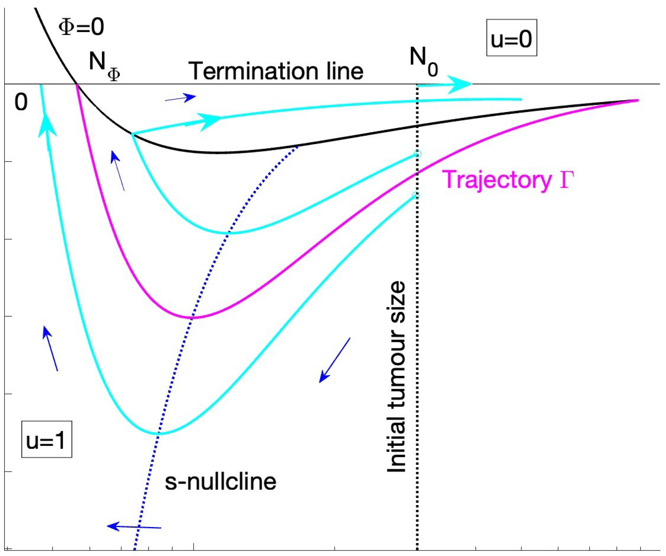
Since the $N,s$ dynamics decouple from those of $W,p_W$, we can consider dynamics in the $(N,s)$ phase plane, with $p_W$ fixed. The switching curve separates the phase plane into two regions, Figure 2, effectively stitching two dynamical systems with $u=0,\mathsf{\Phi }<0$ and $u=1,\mathsf{\Phi }>0$; there may be dynamics on $\mathsf{\Phi }=0$ if there are trajectories on this curve, i.e., singular solutions with ${\displaystyle \frac{\mathrm{d}\mathsf{\Phi }}{\mathrm{d}t}}=0$ and $\mathsf{\Phi }=0$. The flow and optimal trajectories can be determined as follows. We define three curves:

• The switching line $\mathsf{\Phi }=0$ is given by

  $$s_{\mathsf{\Phi }}={\displaystyle \frac{a_0}{{\lambda }_0{N}^2}}-{\displaystyle \frac{\gamma }{p_W{f}_{d1}N}}.$$

  (32)
  Since $f_{d1}\left(0\right)>0$ and finite for $N\in [0,K]$, we have $s_{\mathsf{\Phi }}\to \infty$ as $N\to 0$. There is a unique zero, $N_{\mathsf{\Phi }}$ such that $s_{\mathsf{\Phi }}\left(N_{\mathsf{\Phi }}\right)=0$, i.e., it satisfies $N={\displaystyle \frac{a_0}{{\lambda }_0\gamma }}{p}_W{f}_{d1}\left(N\right)$. Since K is assumed large, and $p_W\le 4e^{-2}{\displaystyle \frac{L_e-L_n}{1-p_0}}$, we have that $N_{\mathsf{\Phi }}\ll K$. It is unique since $f_{d1}$ is monotonically decreasing, $f_{d1}\left(N\right)\le 0$. For $N>N_{\mathsf{\Phi }}$, we have $s_{\mathsf{\Phi }}\left(N\right)<0$. Since $f_{d1}\left(N\right)=f_{d1}\left(0\right)+O\left({\displaystyle \frac{N}{K}}\right)$, we have for $N\ll K$ that

  $$s_{\mathsf{\Phi }}={\displaystyle \frac{a_0}{{\lambda }_0{N}^2}}-{\displaystyle \frac{\gamma }{p_W{f}_{d1}\left(0\right)N}},$$

  (33)

  so there is a local minimum at $N_{minPhi}={\displaystyle \frac{2a_0{p}_W{f}_{d1}\left(0\right)}{{\lambda }_0\gamma }}+O\left(K^{-1}\right)$. We have $f_{d1}\left(N\right)>0$ for $N\in [0,K)$; the drug induced death rate may have a zero, $f_{d1}\left(N\right)=0$ for some $N\ge K$, so $\mathsf{\Phi }$ may also have a local maximum in $[N_{\mathsf{\Phi }},K]$.
• The s-nullcline, $s_{nc}$.

  -

  In the region $u=0$, we have, using (30), that ${\displaystyle \frac{\mathrm{d}s}{\mathrm{d}t}}=-s{\left(N{f}_0\right)}^{\prime }$. Since $N{f}_0$ is concave on $[0,K]$, and zero at $N=0,K$, there exists a unique turning point, $N_{TP}$. The s-nullclines are, thus, $s=0$ and $N=N_{TP}$ where ${\displaystyle \frac{\mathrm{d}\left(N{f}_0\right)}{\mathrm{d}N}}=0$ at $N_{TP}$.

  -

  In the region $u=1$, we have (${\left({\displaystyle \frac{f_{d1}}{N}}\right)}^{\prime }<0$, on interval $[0,K]$),

  $$s_{nc}=-{\displaystyle \frac{a_0}{{\lambda }_0{\left(Nf\right)}^{\prime }}}{\left({\displaystyle \frac{f_{d1}}{N}}\right)}^{\prime }$$

  which has a pole at $N=0$. Thus, this nullcline exists in $u=1$ region where ${\left(Nf\right)}^{\prime }<0$. If ${\left(Nf\right)}^{\prime }=0$ in $[0,K]$, i.e., the population decay under the MTD slows down with N, there may be a second pole.

• The level sets $H(N,s)=h$. We have the following expressions for the Hamiltonian, which is a constant on optimal solutions (PMP).

  $$H=p_{W}sfN+\left(p_W{\displaystyle \frac{a_0}{{\lambda }_0}}{\displaystyle \frac{f_{d1}}{N}}-\gamma \right)u\equiv p_{W}s{f}_{0}N+u\mathsf{\Phi }(N,s)$$

  (34)

  since $\mathsf{\Phi }={\displaystyle \frac{\partial H}{\partial u}}$. Thus, a trajectory on $H=h$ is given by

  $$s_H={\displaystyle \frac{\left(h+\gamma -p_W\frac{a_0}{{\lambda }_0}\frac{f_{d1}}{N}\right)}{p_{W}fN}}.$$

The N-nullclines are $N=0,N=K$ if $u=0$ and $N=0$ if $u=1$. There is, thus, a fixed point $(K,0)$ in the $u=0$ region. Clearly, since ${\displaystyle \frac{\mathrm{d}s}{\mathrm{d}t}}<0$ on $s=0$ if $N>N_{TP}$, the FP is a saddle. There is no fixed point in the $u=1$ region, as ${\displaystyle \frac{\mathrm{d}s}{\mathrm{d}t}}\to \infty$ as $N\to 0$.

Optimal solutions satisfy PMP and, thus, must be a trajectory in our phase space. They start on the line $N=N_0$, and terminate on $s=0$. Since optimal trajectories terminate on $s=0$ in finite time, trajectories can only reach $s=0$ with $u=1$, i.e., they intersect the N-axis with $N\in (0,N_{\mathsf{\Phi }}]$, when $u=0$, $s=0$ is a nullcline and cannot be reached in finite time. In fact the flow suggests trajectories leave the $u=0$ region by crossing the switching curve $\mathsf{\Phi }=0$. Optimal solutions are, thus, trajectories that reach $s=0$ and terminate with $u=1$. We define the trajectory $\mathsf{\Gamma }$ that passes through $(N_{\mathsf{\Phi }},0)$, i.e., reaches the intersection of $s=0$ and $\mathsf{\Phi }=0$. We prove that $\mathsf{\Gamma }$ separates the phase space into trajectories, only trajectories below $\mathsf{\Gamma }$ can terminate.

First, $\mathsf{\Gamma }$ approaches $(N_{\mathsf{\Phi }},0)$ from the $u=1$ region. Consider the trajectories in $u=1$ ($\mathsf{\Phi }>0$) when they cross $s=0$. We have, using (31),

$${\displaystyle \frac{\mathrm{d}\mathsf{\Phi }}{\mathrm{d}t}}={\displaystyle \frac{a_0}{{\lambda }_0}}{p}_W{\left({\displaystyle \frac{f_{d1}}{N}}\right)}^{\prime }{\displaystyle \frac{\mathrm{d}N}{\mathrm{d}t}}-p_W{f}_{d1}N{\displaystyle \frac{\mathrm{d}s}{\mathrm{d}t}}-s{p}_W{\left(f_{d1}N\right)}^{\prime }{\displaystyle \frac{\mathrm{d}N}{\mathrm{d}t}}.$$

Using the dynamics (26), (30), we, thus, have, setting $s=0$,

$${\displaystyle \frac{\mathrm{d}\mathsf{\Phi }}{\mathrm{d}t}}{|}_{s=0}={\displaystyle \frac{a_0}{{\lambda }_0}}{p}_W{\left({\displaystyle \frac{f_{d1}}{N}}\right)}^{\prime }\left(fN+f_{d1}N\right)\equiv {\displaystyle \frac{a_0}{{\lambda }_0}}{p}_W{\left({\displaystyle \frac{f_{d1}}{N}}\right)}^{\prime }{f}_{0}N.$$

This is strictly $<0$ for $N\in (0,N_{\mathsf{\Phi }}]$. Thus, the level set $H=0$ reaches $(N_{\mathsf{\Phi }},0)$ for $u=1$ with $s<0$.

Consider the expression for the Hamiltonian, $H=p_{W}s{f}_{0}N+u\mathsf{\Phi }(N,s)$, then the trajectory $\mathsf{\Gamma }$ that intersects $\mathsf{\Phi }=0$ at $s=0$ lies in the level set $H=0$. We, therefore, have on this trajectory in the $u=1$, $s<0$ region, (using $\mathsf{\Phi }=H-p_{W}s{f}_{0}N$),

$$\mathsf{\Phi }=-p_{W}s{f}_{0}N>0 for N\in (N_{\mathsf{\Phi }},K).$$

At the extremes, $N=N_{\mathsf{\Phi }}$ and $N=K$, we have $\mathsf{\Phi }=0$, i.e., it intersects the switching curve twice, and only twice. Since optimal trajectories must terminate by crossing $s=0$ in the interval $N\in (0,N_{\mathsf{\Phi }}]$, the only optimal trajectories, besides $\mathsf{\Gamma }$, are those that lie below $\mathsf{\Gamma }$, or are already on $s=0$.

The trajectory $\mathsf{\Gamma }$ in fact defines a bang-bang solution with a single switch from $u=1$ to $u=0$. The optimal solution continues in the $u=0$ region on $s=0$ and can have arbitrarily time on $s=0$. These are treat-and-stop solutions, and can be constructed to have arbitrary high horizon times T. The fact that $H=0$ is related to the invariance of the payoff J to extending the horizon time T. Trajectories below $\mathsf{\Gamma }$ terminate in $s=0$, i.e., are MTD solutions; these solutions have a longer horizon time since $N\left(T\right)<N_{\mathsf{\Phi }}$. Finally, there is a branch of no treatment solutions with $u=0$ for all time that start on, and stay on $s=0$. This dynamic on $s=0$ is related to the invariance of the objective to T once drug administration ends.

The case with $b_0=0$ is a special case ($a_0={\lambda }_0$, so no lineage die-out). In this case, $\mathsf{\Phi }=0$ can have a pole at $N=K$, for instance if $f_{d1}=-2d{f}_0$ for a cell cycle drug. The proof still holds by considering only the open region $(0,K)$.

Therefore, we have only three cases for the solutions to PMP:

• No treatment solutions (with $\mathsf{\Phi }\left(t\right)<0$ for all t).
• Treat-and-stop solutions (with $\mathsf{\Phi }\left(t\right)<0$ for $t<x$ and $\mathsf{\Phi }\left(t\right)>0$ for all $t>x$; $x\in \left(0,T\right)$ is the period of drug administration.
• Continuous MTD, $u=1$ throughout the entire therapy (with $\mathsf{\Phi }\left(t\right)>0$ for all t).

Above we considered $p_W$ fixed. For each $p_W$ we have proved that there are three possible branches of solutions: Firstly, the no treatment branch with unrestricted horizon time ($T\ge 0$). Secondly, we have treat-and-stop solutions with $T\ge T_{\mathsf{\Gamma }}$, where

$${\int }_{N_0}^{N_{\mathsf{\Phi }}}{\displaystyle \frac{dN}{f(N,u=1)N}}=T_{\mathsf{\Gamma }}.$$

These solutions exist if $N_{\mathsf{\Phi }}\le N_0$. Finally, we have the MTD solutions with horizon time $T>T_{\mathsf{\Gamma }}$ (if $T_{\mathsf{\Gamma }}$ positive) and $T\ge 0$ when $N_{\mathsf{\Phi }}>N_0$. $p_W$ is determined by the value of G which itself is a function of the dynamics (25) and, thus, on the trajectory $N\left(t\right)$. Thus, for a given horizon time T we need to solve for the initial value $s_0\left(p_W\right)$ that gives the correct horizon time for each value of $p_W$, and then determine $p_W$ by solving the constraint on $p_W$.

We can also prove that for sufficiently small T $\mathsf{\Phi }<0$, and, thus, $u=0$ for $t\in [0,T]$. This follows using the bound $p_N\left(t\right)<-{\displaystyle \frac{a_0{p}_W}{\lambda N{\left(t\right)}^2}}$. We have a sufficiency condition for $\mathsf{\Phi }>0$ ($u=1$) if

$$N<f_{d1}\left(N\right){\displaystyle \frac{a_0{p}_W}{\lambda \gamma }},$$

(35)

where $p_W$ is given by (29). Since $p_W$ is proportional to the TCP, $e^{-{\left({\displaystyle \frac{a_0}{\lambda N\left(T\right)}}+W\left(T\right)\right)}^{-1}}$, it is small for cases where the tumour size cannot be reduced to $O\left(1\right)$ since only then does the TCP increases rapidly. Define $ϵ=e^{-{\left({\displaystyle \frac{a_0}{\lambda N\left(T\right)}}+W\left(T\right)\right)}^{-1}}{|}_{u=1}$ assumed small, (under the MTD $\forall t\in [0,T$]). Then, $p_N=O\left(ϵ\right)$, $p_W=O\left(ϵ\right)$, the former following since ${\displaystyle \frac{\mathrm{d}{p}_N}{\mathrm{d}t}}=O\left(ϵ\right)$, (28). Thus, $\mathsf{\Phi }=-\gamma +O\left(ϵ\right)<0$ for small horizons T, and the optimal solution is no treatment ($u\left(t\right)=0$). When the horizon is sufficiently large, i.e., of order, or larger than ${\int }_{N_0}^1{\displaystyle \frac{dN}{f(N,1)N}}$, then regimens with non-zero $u\left(t\right)$ are possible. The expression (35) then gives a lower bound on the time of the MTD for those solutions with treatment. □

Optimal Controls for Logistic Growth: Numerical Study

We analyse the optimal solutions of the DLP for the specific case of the logistic model and treated with a cell cycle drug,

$${\displaystyle \frac{\mathrm{d}N}{\mathrm{d}t}}=g\left(1-2du\left(t\right)\right)\left(1-{\displaystyle \frac{N}{K}}\right)N,N\left(0\right)=N_0.$$

(36)

Dividing cells are killed by the drug with efficacy $d\in \left(0.5,1\right)$, hereafter referred to as the killing fraction of the drug. The lower bound ensures that the tumour size decays at the MTD. g is the per-capita growth rate of the tumour and K is the tumour’s carrying capacity in the absence of the drug. This has the form (26) with $f_0\left(N\right)=g\left(1-{\displaystyle \frac{N}{K}}\right), f_1\left(N\right)=2dg\left(1-{\displaystyle \frac{N}{K}}\right)$. We set $b_0=0$ for simplicity, i.e., the natural death rate of cancer cells when the tumour size is small is negligible. The birth rate is drug independent by the assumptions above, i.e., $a\left(N\right)=f_0\left(N\right)$, so at low cell density we have $a_0=g,{\lambda }_0=g$. The death rate is solely due to the drug, $b(N,u)=u{f}_1\left(N\right)$, and is density dependent because only cells in cell cycle are killed by the drug, and the cell division rate is density dependent.

The optimal control problem consists of maximising the payoff, (24),

$$J[N,u;T]=\left(L_e-L_n\right){\displaystyle \frac{e^{-{\left(\frac{1}{N\left(T\right)}+W\left(T\right)\right)}^{-1}}-p_0}{1-p_0}}+L_n-\gamma {\int }_0^{T}u\left(t\right)\mathrm{d}t$$

with $p_0=e^{-G{[N,u=0;T]}^{-1}}$, subject to the tumour growth given by Equation (36) and the dynamic of W given by, (20),

$${\displaystyle \frac{\mathrm{d}W}{\mathrm{d}t}}={\displaystyle \frac{g}{N}}\left(1-{\displaystyle \frac{N}{K}}\right),W\left(0\right)=0.$$

(37)

From Theorem 1, we know that all solutions to PMP have $u=1$ (MTD) for an interval $t\in [0,x]$, $x\le T$, the optimal control problem reduces to a one-dimensional optimisation problem of the drug application duration $x\in [0,T]$. By expressing N and W as functions of x, the payoff can be written as:

$$J\left(x\right)=\left(L_e-L_n\right){\displaystyle \frac{e^{-G{\left(\chi \left(x\right)\right)}^{-1}}-p_0}{1-p_0}}+L_n-\gamma x$$

(38)

with $\chi =e^x$, and

$$G\left(\chi \right)={\displaystyle \frac{1}{\left(1-2d\right)}}\left({\displaystyle \frac{1}{N_0}}-{\displaystyle \frac{1}{K}}\right)\left(1-2d{\chi }^{-g(1-2d)}\right)+{\displaystyle \frac{1}{K}}.$$

See Appendix C for derivation. We maximise $J\left(x\right)$ using a sequential quadratic programming method (fmincon solver in matlab). The model parameters were chosen as follows: the growth rate (g) and the carrying capacity (K) of the tumour, were estimated by [31], $g=0.502$ cells/day and $K=1.297\times {10}^9$ cells, respectively. It is assumed that the drug is 100% efficient, so $d=1$. For reference,

Table 1. Parameters used in the tumour evolution models (ODE and BP) and in the DLP formulation.

Parameter	Description
$a_0$	birth rate of cancer cells in the absence of drugs (BP model)
$b_0$	death rate of cancer cells in the absence of drugs (BP model)
${\lambda }_0$	growth rate in the absence of drugs (BP model)
g	tumour growth rate (ODE model)
d	inhibitory effect of the drug on cell division (ODE model)
K	carrying capacity (ODE model)
$L_e$	expected lifetime of a healthy individual
$L_n$	expected lifetime of untreated individual
$\gamma$	influence of drug toxicity on the patient’s expected lifetime.

outlines the key parameters from the tumour evolution model and the DLP.

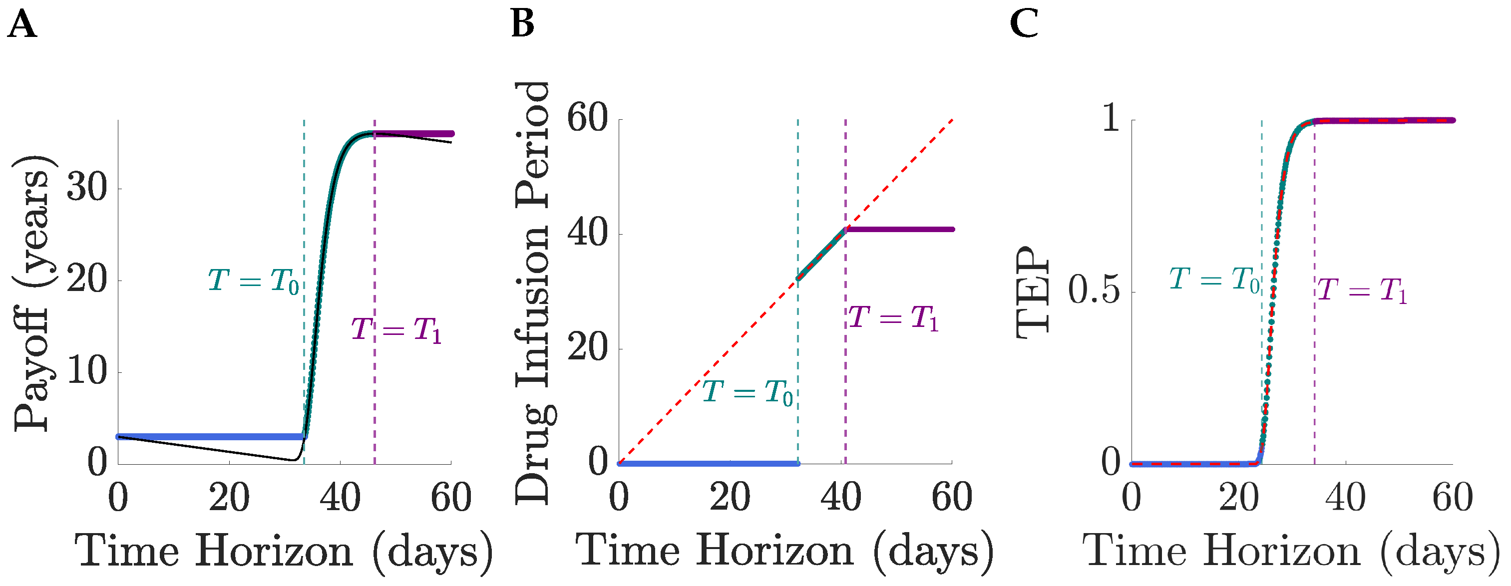
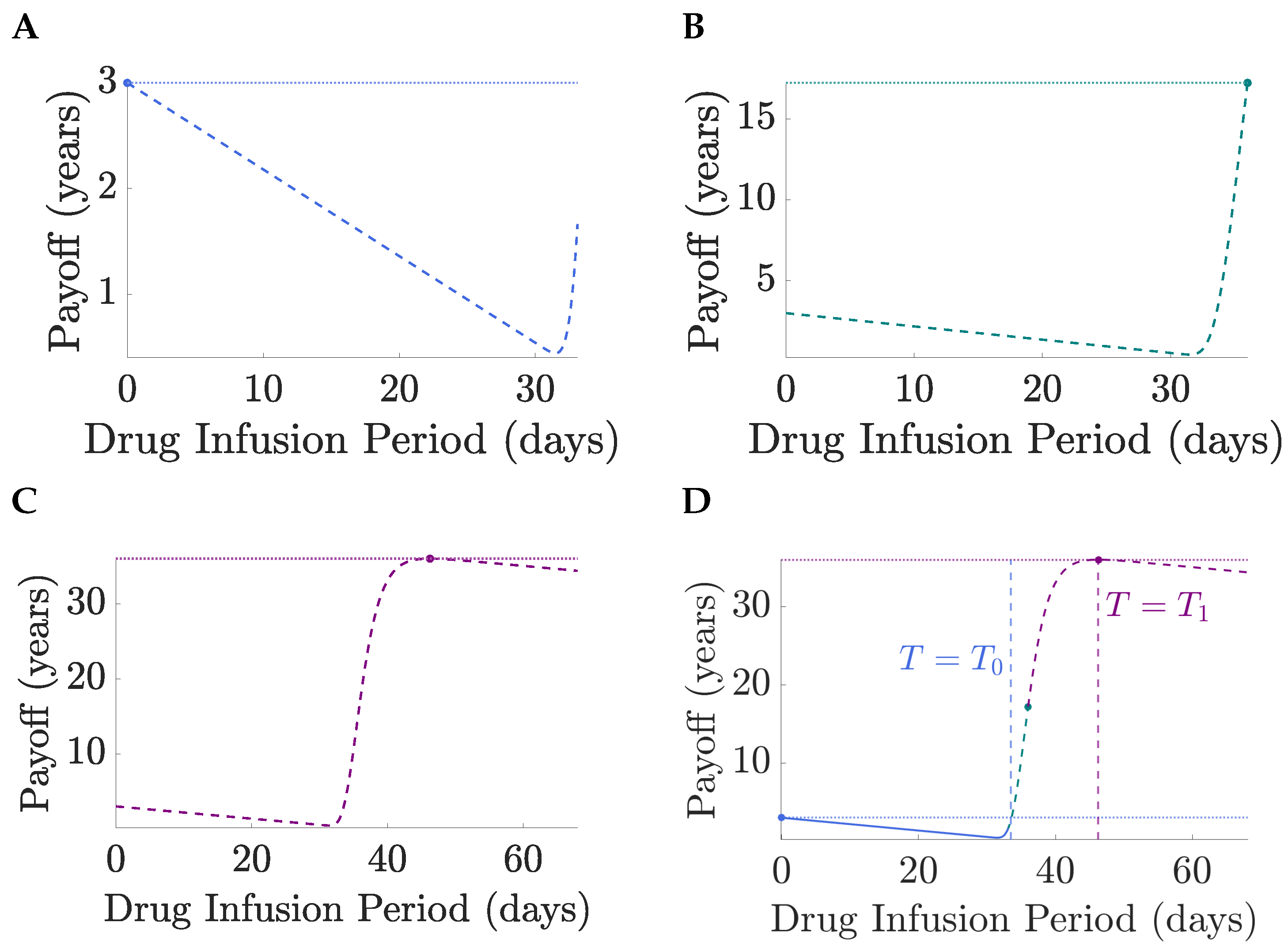
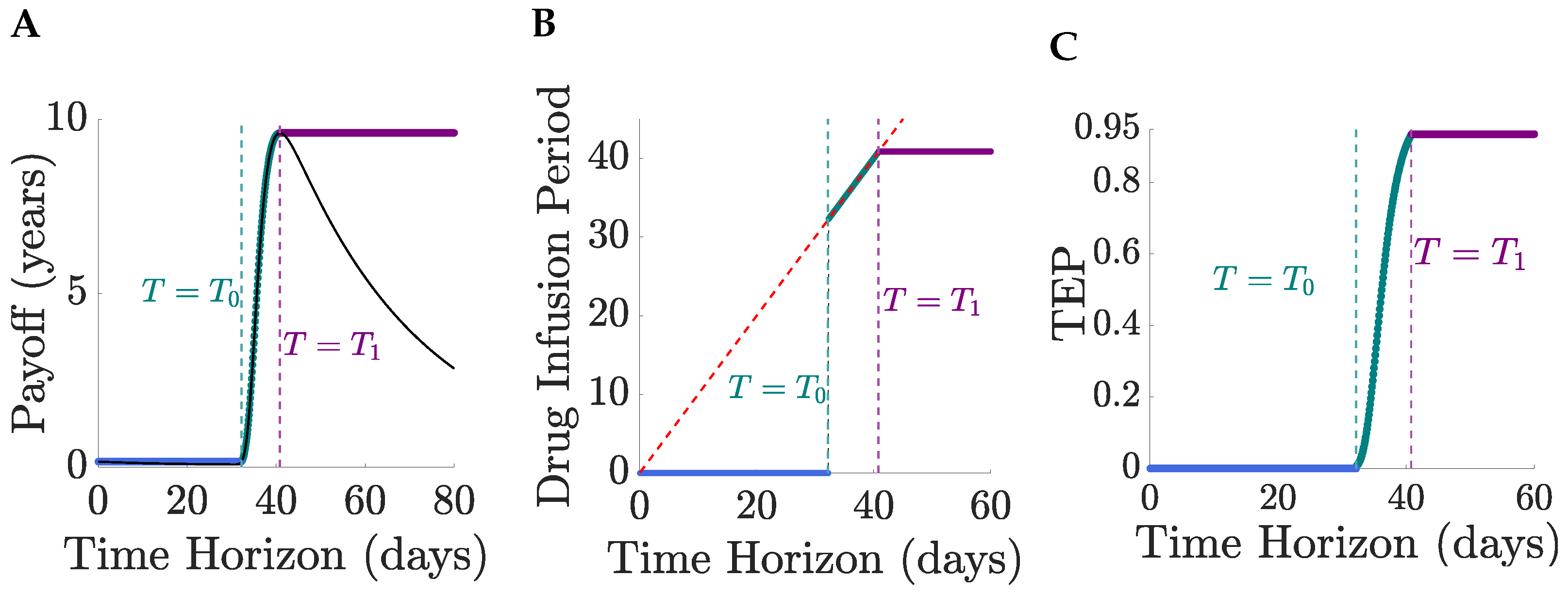
The type of optimal solution (for a fixed initial tumour size $N_0$) is dependent on the degree to which the tumour can be reduced over the horizon time T, Figure 3. Thus, for short horizons, only no treatment solutions exist since the TEP is negligible and toxicity dominates, as proved in the general case, Section 4. At horizon time $T=T_0$, the optimal solution switches to full MTD, the drug infusion period jumping from 0 to T at $T=T_0$, Figure 3B. This is because the pay-off for a continuous MTD regimen is smaller than that for no treatment when $T<T_0$, and crosses it at $T=T_0$, Figure 4, i.e., the TEP is sufficiently high for the expected gain in lifespan to exceed the toxicity costs. At $T=T_1$, continuing at MTD beyond an infusion period $T_1$ is counter productive, toxicity costs again outweigh gains in the TEP which is close to 1 and, thus, cannot be increased much further, Figure 3C. Thus, the optimal solution switches from continuous MTD to treat-and-stop. The optimal infusion period ($x=T_1$) is then independent of the horizon time T as required, Section 3. Thus, for $T>T_1$ the optimal drug regimens are independent of T and the pay-off is constant. Therefore, optimal solutions are limited by a too short-time horizon when $T<T_0$, and for $T_0<T<T_1$ the pay-off (and expected lifespan) can be increased by increasing the time horizon.

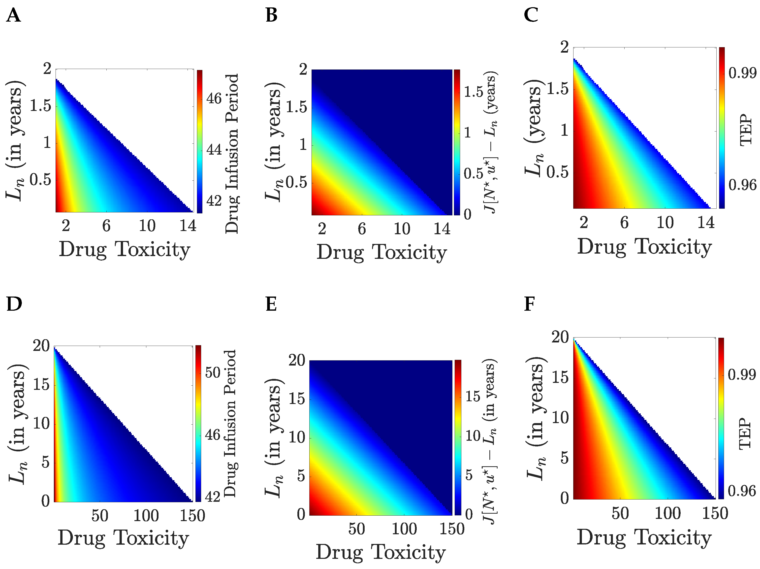
Optimal treatment is explored in Figure 5 against drug toxicity $\gamma$ and the patient lifespan $L_n$ if they are not treated; trends are identical for the cases of a short and long lifespan if the tumour is eliminated, $L_e=2,20$ years. The drug infusion interval decreases as toxicity $\gamma$ increases, and the lifespan gain $L_e-L_n$ decreases, with a critical boundary (in $L_n,\gamma$ space) between untreatable (no treatment is optimal) and treatable patients. The drug infusion period jumps from zero to over 40 days in this case as therapy switches from no treatment to treat-and-stop therapy, Figure 5A,D, with a corresponding jump in the $\mathrm{TEP}$ from 0 to near 1 (in this case over 0.95), Figure 5C,F. Since the drug infusion period is below the time horizon, $T=60$ days, patients in the untreatable category are untreatable for all time horizons. The gain in (discounted) lifespan is approximately linear throughout the treatment range in both $\gamma$ and $L_n$, Figure 5B,E.

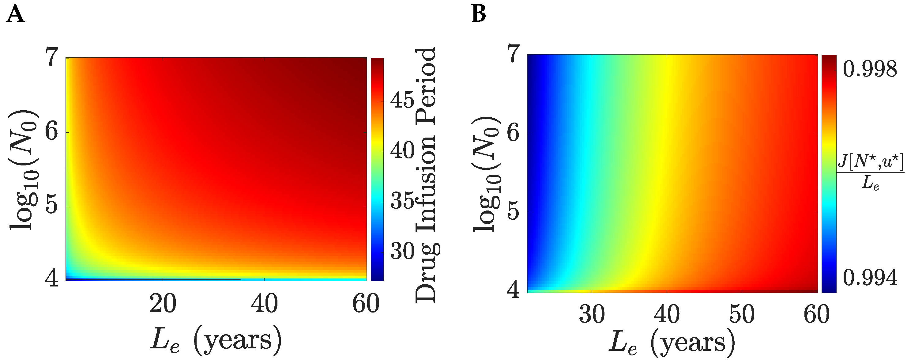
The discounted expected lifespan (DLP) is appropriate for modelling tolerable nausea; severe toxicity costs of therapy are better modelled as SAEs, see Section 5. Under the quality of life interpretation of the DLP we have $\gamma$ order 1. We illustrate optimal solutions for $\gamma =1$. We consider a patient with a short life expectancy under no treatment, $L_n=1$ month, examining therapy for various initial tumour sizes $N_0$ and patient age (assuming an average life expectancy of 85 years, patient age is $85-L_e$ years), Figure 6. For an efficacious drug, the gain in life expectancy is substantial, with life expectancy approximately equal to the life expectancy of a healthy individual (achieving over $99.4\%$ of the life expectancy of a healthy individual), regardless of initial tumour size and $L_e$. The time horizon is $T=60$ days whilst the drug infusion period is 28–49 days, increasing with both the initial tumour size and $L_e$. Thus, all optimal solutions are treat-and-stop and independent of the time horizon. The drug infusion period is only weakly dependent on $L_e$ after a rapid rise, whilst tumour size is the main determinant. All patients are treatable for these parameters ($1\mathrm{year}\le L_e\le 60$ years, $L_n=1$ month, ${10}^4\le N_0\le {10}^7$, $\gamma =1$).

5. Severe Adverse Effects Model: Incorporating Treatment Related Mortality Events

The DLP of Section 4 is only appropriate when toxicity is tolerable. Treatment toxicity can, however, be debilitating, leading to treatment cessation or even death (treatment-related mortality, or TRM) [32]. Adverse effects are graded 1–5 under the common terminology criteria for adverse effects (CTCAE), a classification managed by the Cancer Therapy Evaluation Programme [33]. Grades 1 and 2 are mild, serious adverse effects are 3–5, grade 3 events may require hospitalisation, grade 4 is life threatening and in need of urgent medical care, and grade 5 is death through an adverse event. Thus, the negative effects of treatment can be incorporated as a SAE event, causing cessation of treatment and/or death.

Here we consider the event of patient death through TRM, with other events, such as tumour elimination. TRM is modelled as a Poisson processes with rate $\mu (u,t)$, assumed a function of time and the current drug concentration. The expected patient lifetime is then given by

$$J[N,u;T]=(1-p_d[N,u;T])\sum _{k=1}^n{p}_k[N,u;T]L_k+{\int }_0^{T}t\mu (u\left(t\right),t)\left(exp-{\int }_0^t\mu (u\left(s\right),s)ds\right)dt$$

(39)

comprising two terms corresponding to the events of surviving therapy, with probability $1-p_d[N,u;T]$, and TRM, with probability $p_d[N,u;t]$, respectively. The last term is the expected lifetime conditioned on TRM. Here $p_d[N,u;t]=1-exp\left(-{\int }_0^t\mu (u\left(s\right),s)ds\right)$ is the probability of death caused by treatment over time t. Generally we can have multiple possible futures $k=1,\dots ,n$ with expected lifetimes $L_k$. Only if the patient survives treatment are these events relevant. There is, thus, a dependence hierarchy; survival depends on $u\left(t\right)$ only (and is independent of the other events), and the other events (can) depend on the state history $\left(N\right(t),u(t\left)\right)$.

5.1. Logistic Tumour Growth with TRM Treated with a Cell Cycle Targeting Drug

Here we explore optimal solutions for the logistic tumour evolution model treated with cell cycle targeting drugs, i.e., tumour dynamics (36) supplemented with the BP birth rate a as in Section 4 (i.e., independent of the drug). We assume that the patient death rate due to the drug is proportional to the amount of drug administered and is given by $\mu =\alpha u$, with $\alpha ={\displaystyle \frac{1}{\tau }}$, and $\tau$ the expected period a patient can survive under continuous MTD drug administration, hereafter referred to as the drug tolerance interval. We consider three outcomes at the time horizon: the patient does not survive treatment (TRM), cure (tumour clearance and survival to T), and failure to eliminate the tumour, so the patient will eventually relapse. As before, we assume $L_n>T$. The payoff with these three outcomes is:

$$J[N,u;T]=e^{-\alpha {\int }_0^{T}u\left(t\right)\mathrm{d}t}\left(L_e{p}_e[N,u;T]+L_n\left(1-p_e[N,u;T]\right)\right)+{\int }_0^T\alpha t{e}^{-\alpha {\int }_0^{t}u\left(s\right)\mathrm{d}s}u\left(t\right)\mathrm{d}t,$$

(40)

where $p_e[N,u;T]$ is the treatment dependent elimination probability, TEP, (23). The parameter values for the tumour dynamics (ODE model and BP model) are as in Section 4. The parameters used for the SAP are outlined in

Table 2. Parameters used in the SAP formulation.

Parameter	Description
$L_e$	expected lifetime of a healthy individual
$L_n$	expected lifetime of untreated individual
$\alpha$	Proportionality constant linking drug quantity u to TRM rate $\mu$ ($\mu =\alpha u$).
$\tau$	the drug tolerance interval (the expected period a patient can survive under continuous MTD drug administration, i.e., $\tau ={\displaystyle \frac{1}{\alpha }}$).

, whereas the tumour evolution parameters are outlined in Table 1.

Applying PMP, the optimal solutions are bang-bang, and as with the DLP there can only be three types of solutions: no treatment, the MTD for the full horizon, and treat-and-stop solutions (at the MTD), proof in Appendix D. We numerically determined optimal solutions using a direct method for bang-bang solutions, see Appendix E; specifically, the control is piece-wise constant taking only the values 0 or 1 on a partition of $[0,T]$. A sequential quadratic programming (SQP) method (Matlab fmincon solver) was utilised to determine the optimal switching times.

Similar to Section 4, for small time horizons optimal solutions are no treatment, $T<T_1$, continuous MTD for intermediate horizons, $T_1<T<T_2$, and treat-and-stop solutions for large horizons, $T>T_2$. For large enough time horizons, T, the optimal solutions are independent of T and all optimal treat-and-stop solutions have an identical drug regimen, Figure 7.

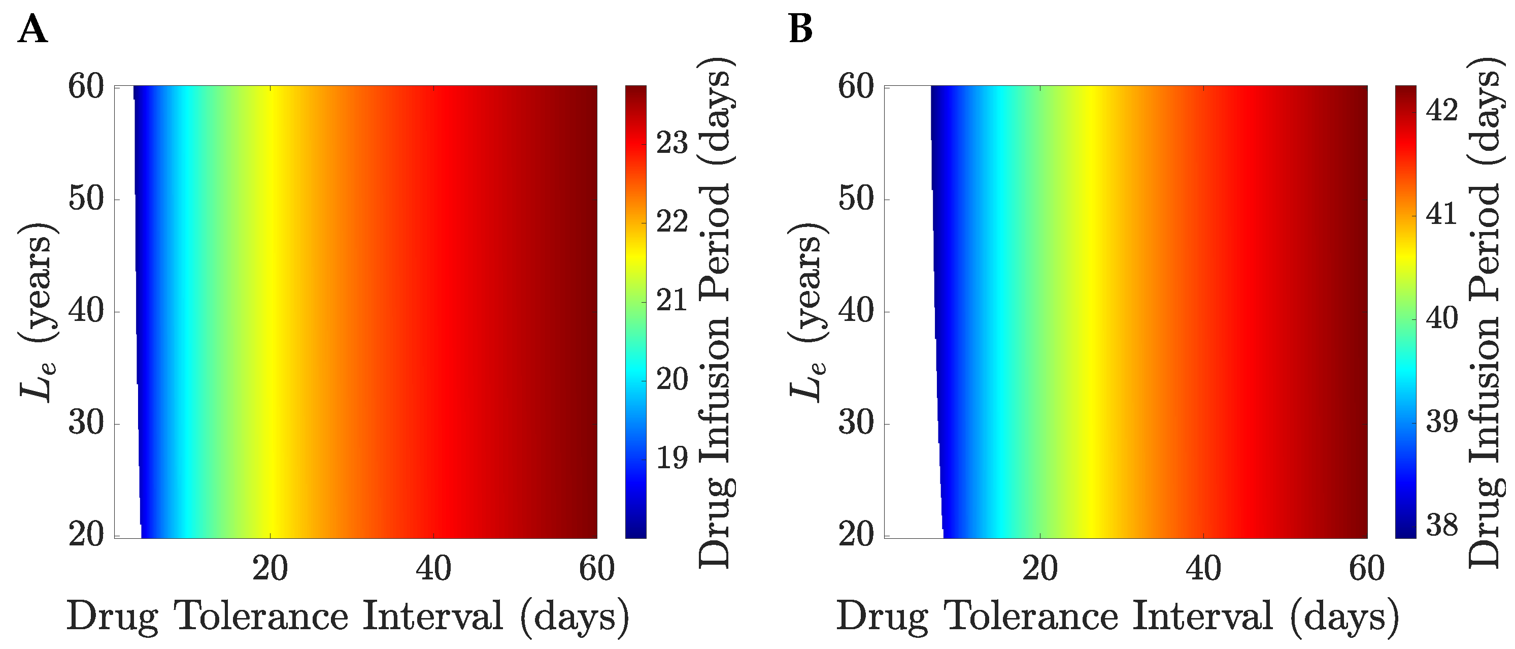
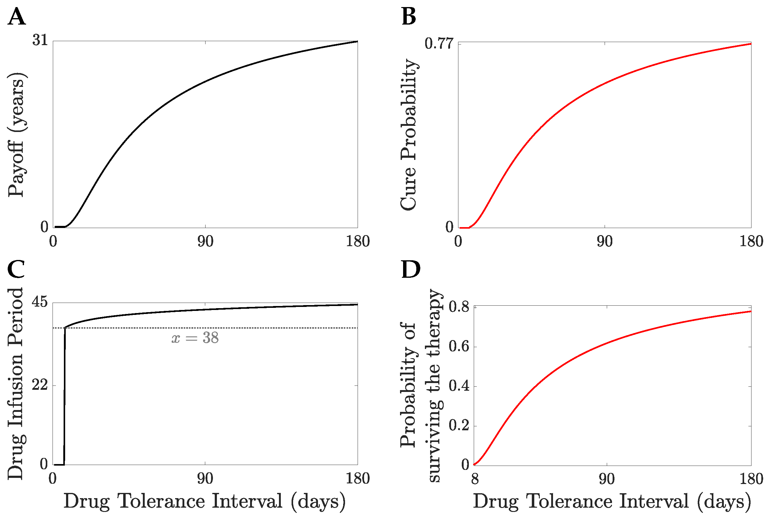
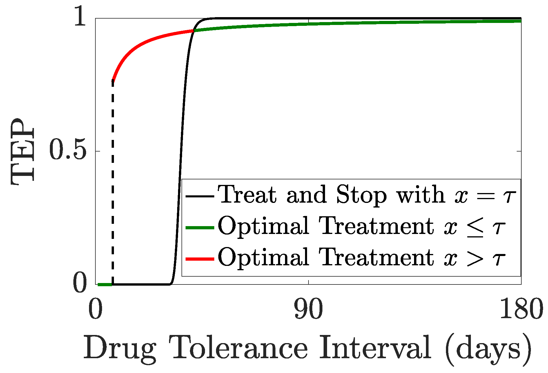
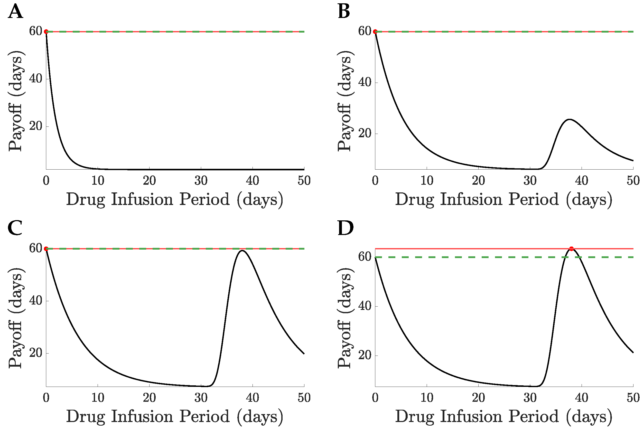
We illustrate the TRM model with $L_e=40$ years and $L_n=2$ months, Figure 8. The patient’s life expectancy, the optimal drug administration period, the patient’s survival probability and the cure probability increase with $\tau$, Figure 8. For $\tau <180$ days, the probability that a patient survives therapy is close to $0.78$, Figure 8B with a TEP post-treatment in excess of $0.72$, Figure 9. Patients can be divided into a treatable and an untreatable category based on the value of the drug tolerance interval, $\tau$; patients are treatable only if they can survive continuous MTD drug administration for 7 days or longer, Figure 8C; these patients are treated with the MTD for a minimum of 38 days, Figure 8C. Thus, there exists a critical value of the drug tolerance interval, $\tau ={\tau }_{\mathrm{crit}}$, where the optimal drug administration period jumps from 0 to a non-zero value. Despite the abrupt change in the optimal drug administration period, the patient’s life expectancy under optimal treatment remains continuous at the critical threshold $\tau ={\tau }_{\mathrm{crit}}$ Figure 8A,C. A comparison of no treatment to the MTD is shown in Figure 10 for $\tau <{\tau }_{crit}$ and $\tau >{\tau }_{crit}$, the switch of solution causing a jump in the drug infusion period whilst retaining continuity in the pay-off. MTD drug administration has a local maximum in the payoff with drug infusion period that becomes the global maximum at $\tau ={\tau }_{crit}$, Figure 10, having a payoff $J[N,u=0;T]=L_n$.

Patients in the treatable category with low drug tolerance intervals $\tau$ receive treatment for a duration exceeding their expected survival time under continuous MTD administration, Figure 9. The optimal drug administration period increases with $\tau$, but becomes eventually shorter than $\tau$. Thus, at low values of $\tau$, optimal drug strategies focus on achieving tumour elimination despite high TRM risks. In contrast, at high values of $\tau$, tumour control is more readily achieved, and drug toxicity becomes the primary factor limiting the infusion period.

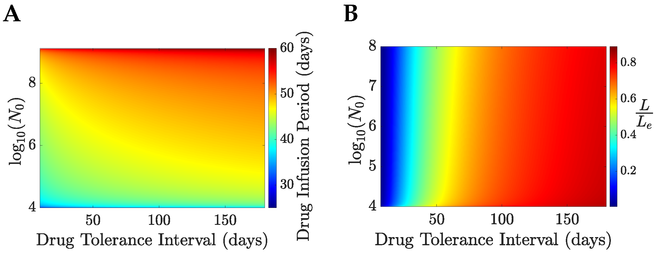
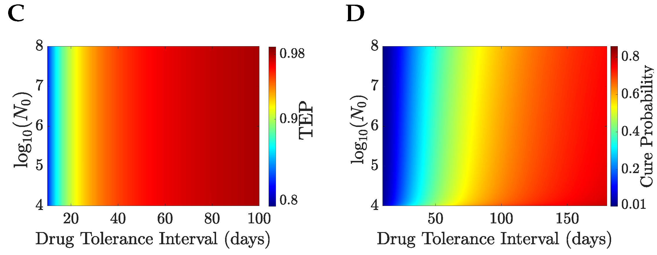
The optimal drug administration period, x, increases with both the initial tumour size ($N_0$) and the drug tolerance interval ($\tau$), Figure 11A; the strong dependence of $N_0$ on x is not surprising as the tumour needs to be reduced to the order of a few cells before elimination is feasible. The TEP is almost independent of $N_0$ for fixed $\tau$ and is strictly increasing with $\tau$, taking values larger than $0.8$, Figure 11C; this is achieved by the total amount of drug increasing with the initial tumour size. The cure probability increases with $\tau$ with a shallow decrease with the initial tumour size, Figure 11D; this is because of the decreasing probability of the patient survival under a longer drug administration period. The cure probability and the relative life expectancy under optimal treatment have similar dependence on $N_0,\tau$, taking similar values Figure 11B,D. Dependence of the optimal solutions on $L_e$, or age, can also be explored, Appendix F. Dependence on age is weak.

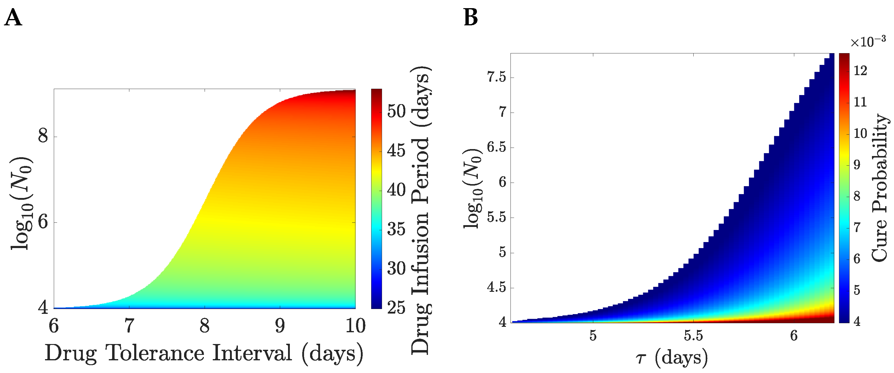
Patients can be subdivided into a treatable and an untreatable class, based on the drug tolerance interval and the size of the tumour prior to therapy, Figure 12. Treatable patients, who are characterised by $(\tau ,N_0)$ values that are close to the boundary of the two classes, are treated with large periods of MTD drug administration (spanning from 25–50 days), Figure 12A, whereas the cure probability is of the order of ${10}^{-2}$, Figure 12B. Optimal drug regimens favour the objective of eliminating the tumour over the objective of retaining low levels of drug toxicity. Because $L_e$ is equal to 40 years and $L_n$ is 2 months, the potential gain in life expectancy under drug administration can be much larger than the life expectancy under no treatment, even when the cure probability is small.

5.2. Intermediate SAE and Iterative Therapy Under LEP Optimisation

SAEs can lead to cessation of treatment for a period of time or a shift to another treatment, for instance the maximum drug dose could be reduced, or a less intensive drug used. Treatment with cessation events, thus, occurs in phases, phase j having $j-1$ previous SAE events. The objective is formulated as follows. We define the expected patient lifespan for each phase of treatment, i.e., $J_s^{\left(j\right)}[N,\overrightarrow{u};T]$ is the expected lifespan after $j-1$ SAEs, with the last occurring at time $s\in [0,T]$; phase j, thus, starts at time s with tumour size $N\left(s\right)$ determined by the treatment before s. Here the drug concentration is a vector, $\overrightarrow{u}\left(t\right)$, with the patient being treated with drug concentration $u_j\left(t\right)$ (component j) in the $j$th treatment phase, which could in fact be the same drug but with a reduced MTD.

Consider the case with a potential SAE event with dose dependent rate $\alpha u_1\left(t\right)$, that causes the current therapy to cease and a switch to an alternative therapy, drug concentration $u_2\left(t\right)$. We assume this alternative treatment is not subject to the possibility of an SAE. Similar to the case of TRM, (40), we have the expected lifespan,

$$\begin{array}{ccc}\hfill J[N,\overrightarrow{u};T]& =& e^{-\alpha {\int }_0^T{u}_1\left(s\right)\mathrm{d}s}\left(L_e{p}_e[N,\overrightarrow{u};T]+L_n\left(1-p_e[N,\overrightarrow{u};T]\right)\right)\hfill \\ & & +{\int }_0^T\alpha u_1\left(s\right)\left(t\right)e^{-\alpha {\int }_0^t{u}_1\left(s\right)\mathrm{d}s}{J}_t^{\left(2\right)}[N,\overrightarrow{u};T]\mathrm{d}t,\hfill \end{array}$$

(41)

where $p_e[N,\overrightarrow{u};T]$ is the treatment dependent elimination probability, TEP, (23), and $J_t^{\left(2\right)}[N,\overrightarrow{u};T]$ is the expected lifespan conditioned on switching to treatment 2 at time t. This is an adaptive therapy, since an SAE is an observation event that changes the therapy if it occurs.

To compute the expected lifetime (41), we, therefore, need to solve for the optimal treatment $u_2\left(s\right),s>t$, for any SAE time t, initial tumour size $N\left(t\right)$, by maximising the conditional LEP,

$$J_t^{\left(2\right)}[N,\overrightarrow{u};T]=t+(L_e-t)p_{eSAE}[N,\overrightarrow{u};t,T]+(L_n-t)\left(1-p_{eSAE}[N,\overrightarrow{u};t,T]\right)$$

where $L_e$ is the expected lifespan on tumour elimination, $L_n$ is the expected lifespan if the tumour is not eliminated, and $p_{eSAE}[N,\overrightarrow{u};t,T]$ is the probability of tumour (lineage) elimination conditioned on an SAE at t. In practice, the SAE may affect these lifetimes. We, thus, have a complex iterative optimisation problem. To accommodate SAE grade, rates for each grade of SAE would need to be defined, whilst allowing for multiple phases of treatment (multiple SAEs) would further extend the iterative depth.

6. Conclusions

We have proposed a new optimal control criterion for determining optimal chemotherapy scheduling and doses within the context of key events affecting outcome, such as tumour elimination (cure, if patient survives treatment) and patient death through TRM. We propose that maximising the patient’s life expectancy by averaging over all possible outcome events is a realistic interpretation of the objective of therapy, i.e., is a quantifiable measure of the best patient outcome. We developed the proposal within a deterministic modelling framework based on the rate of event occurrences, such as tumour elimination. The life expectancy pay-off is very general; here, we illustrated its use on chemotherapy with three possible events (cure, failure to clear tumour cells, and TRM) whilst it can be generalised to include surgery, transplant, combination therapy, adaptive therapy, and multiple stage therapy. Tumour growth dynamics (both with and without therapy), and the event rates need to be parametrised, specifically the life expectancy and SAE rates in terms of therapy parameters. Thus, for chemotherapy we need to incorporate drug mechanism and drug efficacy into the tumour dynamics, and the rate of TRM. Parametrised tumour models have been developed, [11,34,35,36], whilst TRM rates, [32,37,38] and survival data (overall survival and progression free survival) may allow these additional parameters to be estimated. Incorporating other events will need their rates and dependence on tumour characteristics, such as size and replication rate and therapy to be determined. If parametrisation includes patient demographics then this is a natural framework for personalised therapy optimisation.

The optimisation criterion we propose addresses various challenges in the field of applied optimal control for cancer chemotherapeutics, and offers a number of advantages over previous formulations, Table 3. To our knowledge, there has been no previous attempt in the literature to formulate an optimal control problem that considers tumour characteristics after therapy; typically, the performance criteria for evaluating a therapy’s anti-tumour efficacy is based on the tumour’s state at the end of treatment. Our lifetime expectancy pay-off addresses this issue by modelling stochastic events during therapy, including tumour elimination, events that determine patient prognosis. Therefore, our formulation inherently incorporates considerations post-treatment horizon, and in fact quantifies the probability of each outcome (set of events). Being based on the expected lifespan, the lifetime payoff has two additional attractive properties. Firstly, the optimal solutions are independent of the horizon time T once drug application ceases. In effect, provided a sufficiently large horizon time is used, all solutions are then independent of T. To our knowledge no other optimal cancer therapy (finite time horizon) control problem has this property. Secondly, our objective has no subjective free parameters as it is interpretable. This contrasts to traditional approaches of cancer therapy optimisation that frame it as a multiple objective optimisation problem. For instance, the two competing objectives of controlling the tumour size and limiting the impact of toxicity to the patient are often combined as a weighted sum [1,9]. A drawback of this method is that the weights are arbitrary, and it is hard to give a biological justification for a given choice of the weights. Balancing multiple competing objectives can also be analysed using Pareto optimality [39,40] that delays making subjective choices; a solution is Pareto optimal if no objective can be improved without compromising another. Solving the Pareto optimisation problems involves identifying all Pareto-optimal solutions, which defines the Pareto front. A Pareto optimal solution is then subjectively selected, either based on the decision maker’s preferences or utilising additional factors that could include patient input. However, as with traditional objective weighting methods, solutions determined by Pareto optimisation depend on the optimisation parameters, [41], and, therefore, depend on subjective choices. In the LEP formulation, all competing therapy objectives are inherently weighted by the event-probabilities (e.g., tumour elimination) that have direct biological interpretations; there is, thus, a single objective: the patient’s expected lifetime averaged over all therapy outcomes to be maximised. The LEP’s advantages are summarised in Table 3.

Two life expectancy pay-off models were presented and analysed, where DLP can be considered a tolerable toxicity model and SAP a model of severe toxicity. Both models incorporate the event of tumour elimination, i.e., patient cure, and are illustrated on a one-compartment tumour model with a cell cycle targetting drug. In DLP, chemotherapy can reduce significantly the patient’s quality of life, and, thus, we proposed a discounted pay-off to model that poor quality of life during therapy, [26]. In SAP, drug-induced death is modelled as a Poisson process with rates proportional to the amount of drug administered at any time point of the treatment. For both optimisation problems we proved that (1) optimal solutions are bang-bang, and (2) every solution that satisfies PMP has at most one switch and can only switch from continuous MTD to no drug at some time point x. Since PMP is a necessary condition for optimality, finding the optimal solution reduces to determining the optimal switching time x, where the control transitions from the MTD to no drug. This reduces the original optimal control problem to a one-dimensional NLP problem.

In both of these models, patients are either treatable or untreatable. In our analysis, treatability was dependent on tumour characteristics, such as size, and patient characteristics, such as their expected lifetime without treatment ($L_n$) and tolerability to drug toxicity, Figure 5 and Figure 12. More generally, we would expect that treatability would be dependent on tumour type and stage. A personalised LEP approach would, thus, allow this information to be incorporated and patient specific therapy designed. Provided the time horizon is large enough treatability is independent of the time horizon and treatment switches from no treatment to treat-and-stop.

Optimal solutions of both payoffs prioritise tumour elimination over low total drug toxicity. At the untreatable boundary the optimal drug administration period jumps from 0 days to a period large enough to achieve a large TEP (for the parameters used in this study, treatable patients have a $\mathrm{TEP}>0.8$); this is because the potential gain in life expectancy, when the tumour is eliminated, is much greater than the life expectancy when treatment does not eliminate the tumour. In particular, in SAP treatable patients close to the untreatable boundary can have a cure probability smaller than $0.02$, with drug administration exceeding 20 days (Figure 12). For the parameters used here, treatable patients under optimal treatment have an expected lifetime that spans from 10–83% of the life expectancy of a healthy individual Figure 11B. This high variability depends primarily on the initial tumour size and the drug tolerance interval $\tau$, since patients that are more susceptible to the drug are more likely to die during therapy. In the DLP, the life expectancy of a treatable patient is nearly identical to that of a healthy individual—exceeding 99.4% of a healthy individual, Figure 6B.

In general, SAEs significantly disrupt the course of treatment, potentially leading to an interruption of treatment, [42], a permanent cessation of treatment with a shift to palliative care [43] or TRM [44]. We presented a SAP model based on TRM, but it can be modified to account for SAE that causes treatment to be ceased or modified. Since treatment is modified based on an observation (SAE event), this comprises an adaptive therapy. This SAE interuption of therapy then gives an iterative optimisation problem involving conditional subproblems with a SAE at time $t\in [0,T]$, see Section 5.2.

We illustrated the lifetime expectancy pay-off for chemotherapy optimisation of simple tumour growth models with only two events (cure, TRM). This has the advantage of avoiding the need to describe and justify detailed cancer models, thus, allowing the pay-off formulation to take centre stage. Further, the models are sufficiently simple to allow formal analysis, in particular we proved that optimal solutions are treat-and-stop. Other types of solutions, such as delayed treatment [1,20,45] or administrating the highest drug dose at the end of the treatment period [46,47], have been found to be optimal in a number of theoretical studies, solutions that are clinically ill advised. So it is reassuring that our pay-off gives clinically suitable solutions; how robust this is for more realistic tumour growth models and additional events is unclear and needs to be examined.

The LEP framework is very flexible, and can be generalised in multiple ways, including incorporating other treatments, such as radiotherapy and surgery, more complex cancer growth models [8,48], including multi-compartment models, additional events such as mutation and metastasis, and more realistic drug mechanism models with more realistic application schedules (discrete injections) and pharmacokinetics/dynamics. To incorporate additional events, the event rates ${\mu }_k(N,u)$ need to be parametrised (with dependence on the tumour size and drug). However, because we classify outcomes by tumour elimination, we need to also allow for the time of elimination during therapy, since if eliminated the event rate changes to ${\mu }_k(0,u)$. Thus, we need to have the joint event of tumour elimination and the event; this will be pursued elsewhere. These generalisations will likely pose optimisation problems where the PMP equations (the TPBVP) cannot be solved analytically, and, thus, bang-bang solutions are not assured. Numerical methods are then needed [49,50] that either produce solutions to PMP (so called indirect methods), or direct methods that approximate the control function using a linear combination of basis functions (e.g., Lagrange polynomials or piece-wise constant functions), giving a finite-dimensional non-linear programming (NLP) problem. There are efficient NLP-solver algorithms in the literature, many of which are open source [51,52].

The LEP framework has the potential for application in real-world cancer therapy, for instance, in personalised therapy, supporting clinical decision making by identifying how different patient groups might benefit most effectively from therapy, and determining the most effective treatment in fragile patients, thereby reducing overtreatment. AML for example is typically treated with intensive therapy, but older patients may be treated with less intense, less effective therapy [53,54,55,56]. Having a clinical diagnostic tool to ascertain best therapy based on patient health and other factors would potential transform geriatric AML treatment. However, although the LEP has a key advantage over standard cancer treatment cost functions in that it is objective and the parameters have direct interpretations, there remains the difficulty of determining those parameters from real world data. Three types of data are required. Most accessible is life expectancy data, such as from life tables that typically allow for multiple covariates, including race, socio-economic status [57], and comorbidities [58]. Survival (Kaplain–Meyer) curves can potentially be used to structure expected lifespan by cancer subtype, grade, and stage, although data to determine average lifespan in the absence of treatment is likely rare. Data on causes of deaths across different cancers is also available [59]. Secondly, the rates of the possible events is needed, with dependency on tumour size and drug concentration; tumour size is known to be a prognostic factor in many cancers, playing a key role in cancer stage, although likely a prognostic factor alone in many cancers (hepatocellular carcinoma [60], breast cancer [61,62], and NSCLC [63,64]). Finally, tumour growth and death rates are needed both in the presence and absence of the drug(s). Growth dynamics and drug efficacy is extremely complex for solid tumours, given the genetic and environmental heterogeneity of the tumour [65], whilst the growth dynamics of leukaemias is better characterised [10,11,66,67,68]. Developing predictive models for key events in cancer is a growing field; thus, as these improve, the LEP framework will be far more tractable.

The primary objective of this work was to develop a novel deterministic payoff functional that quantifies a patient’s expected lifetime under different therapy outcomes, incorporating the negative impact of excessive drug toxicity on life expectancy. As an initial step toward studying this objective, simple one-compartment tumour growth models were considered. Future extensions may incorporate detailed tumour models, drugs, and detailed pharmacokinetics/pharmacodynamics. In the case of blood cancers, multi-compartment models are usually employed to describe different levels of hierarchies in the blood maturation process in both cancer and healthy cell lineages. In the case of solid tumours spatial heterogeneity should be addressed, since cells that are in a hypoxic environment tend to be more resistant to the drug compared to non-hypoxic cells. Spatial heterogeneity is usually addressed by PDE models since spatio-temporal characteristics of the tumour should be considered. Our formulation should apply to all these extensions.

Table 3. Therapy optimisation formulations.

Context	Formulation	Optimisation Approach	Parameters	Post-Horizon Outcomes	Dependence on Horizon
Optimise drug therapy over dose, timings, and combinations.	Multiple competing objectives, defined by objective functions $J_i,i=1\dots n$.	Minimise weighted sum ${\sum }_{i=1}^n{w}_i{J}_i$, arbitrary weights $w_i$ [1,5,9].	$w_i$ and $J_i$ subjectively chosen.	Not normally considered [5].	Yes.
		Pareto optimisation [40].	Subjective choice of $J_i$, and subjective selection of best solution on Pareto front.
Optimise drug therapy over dose, timings, and combinations.	Maximise patient lifespan.	Life expectancy pay-off (LEP).	Event rates and lifespan conditioned on events need to be determined from data.	Classified by events, for instance including cure, relapse, death.	Invariant provided therapy ended.
Optimise over choice of defined treatments.	Maximise patient lifespan	Dynamic treatment regime models [24,69].	Treatment outcome statistics required from data.	Various, including cure, relapse, death.	Not relevant

Table 3. Therapy optimisation formulations.

Context	Formulation	Optimisation Approach	Parameters	Post-Horizon Outcomes	Dependence on Horizon
Optimise drug therapy over dose, timings, and combinations.	Multiple competing objectives, defined by objective functions $J_i,i=1\dots n$.	Minimise weighted sum ${\sum }_{i=1}^n{w}_i{J}_i$, arbitrary weights $w_i$ [1,5,9].	$w_i$ and $J_i$ subjectively chosen.	Not normally considered [5].	Yes.
		Pareto optimisation [40].	Subjective choice of $J_i$, and subjective selection of best solution on Pareto front.
Optimise drug therapy over dose, timings, and combinations.	Maximise patient lifespan.	Life expectancy pay-off (LEP).	Event rates and lifespan conditioned on events need to be determined from data.	Classified by events, for instance including cure, relapse, death.	Invariant provided therapy ended.
Optimise over choice of defined treatments.	Maximise patient lifespan	Dynamic treatment regime models [24,69].	Treatment outcome statistics required from data.	Various, including cure, relapse, death.	Not relevant

References

1. Schattler, H.; Ledzewicz, U. Optimal Control for Mathematical Models of Cancer Therapies An Application of Geometric Methods; Lecture Notes in Biomathematics; Springer: Berlin/Heidelberg, Germany, 2015; Volume 42. [Google Scholar]
2. Swan, G.W. Optimization of Human Cancer Radiotherapy; Interdisciplinary Applied Mathematics; Springer: Berlin/Heidelberg, Germany, 2015. [Google Scholar]
3. Martin, R.; Te, K.L. Optimal Control of Drug Administration in Cancer Chemotherapy; World Scientific Publishing Company Pte. Ltd.: Singapore, 1994. [Google Scholar] [CrossRef]
4. Kimmel, M.; Swierniak, A. Control Theory Approach to Cancer Chemotherapy: Benefiting from Phase Dependence. Tutorials in Mathematical Biosciences III: Cell Cycle, Proliferation, and Cancer; Springer: Berlin/Heidelberg, Germany, 2005; pp. 185–221. [Google Scholar]
5. Engelhart, M.; Lebiedz, D.; Sager, S. Optimal control for selected cancer chemotherapy ODE models: A view on the potential of optimal schedules and choice of objective function. Math. Biosci. 2011, 229, 123–134. [Google Scholar] [CrossRef] [PubMed]
6. Shi, J.; Alagoz, O.; Erenay, F.S.; Su, Q. A survey of optimization models on cancer chemotherapy treatment planning. Ann. Oper. Res. 2014, 221, 331–356. [Google Scholar] [CrossRef]
7. Rojas, C.; Belmonte-Beitia, J. Optimal control problems for differential equations applied to tumor growth: State of the art. Appl. Math. Nonlinear Sci. 2018, 3, 375–402. [Google Scholar] [CrossRef]
8. Kuznetsov, M.; Clairambault, J.; Volpert, V. Improving cancer treatments via dynamical biophysical models. Phys. Life Rev. 2021, 39, 1–48. [Google Scholar] [CrossRef] [PubMed]
9. Jarrett, A.M.; Faghihi, D.; Hormuth, D.A.; Lima, E.A.; Virostko, J.; Biros, G.; Patt, D.; Yankeelov, T.E. Optimal control theory for personalized therapeutic regimens in oncology: Background, history, challenges, and opportunities. J. Clin. Med. 2020, 9, 1314. [Google Scholar] [CrossRef]
10. Guzev, E.; Jadhav, S.S.; Hezkiy, E.E.; Sherman, M.Y.; Firer, M.A.; Bunimovich-Mendrazitsky, S. Validation of a Mathematical Model Describing the Dynamics of Chemotherapy for Chronic Lymphocytic Leukemia In Vivo. Cells 2022, 11, 2325. [Google Scholar] [CrossRef]
11. Hoffmann, H.; Thiede, C.; Glauche, I.; Bornhaeuser, M.; Roeder, I. Differential response to cytotoxic therapy explains treatment dynamics of acute myeloid leukaemia patients: Insights from a mathematical modelling approach. J. R. Soc. Interface 2020, 17, 20200091. [Google Scholar] [CrossRef]
12. Zhu, C.; Stiehl, T. Modelling post-chemotherapy stem cell dynamics in the bone marrow niche of AML patients. Sci. Rep. 2024, 14, 25060. [Google Scholar] [CrossRef]
13. Yin, A.; Moes, D.J.A.; van Hasselt, J.G.; Swen, J.J.; Guchelaar, H.J. A review of mathematical models for tumor dynamics and treatment resistance evolution of solid tumors. CPT Pharmacomet. Syst. Pharmacol. 2019, 8, 720–737. [Google Scholar] [CrossRef]
14. Ledzewicz, U.; Schättler, H. On the Role of the Objective in the Optimization of Compartmental Models for Biomedical Therapies. J. Optim. Theory Appl. 2020, 187, 305–335. [Google Scholar] [CrossRef]
15. Katta, B.; Vijayakumar, C.; Dutta, S.; Dubashi, B.; Ramakrishnaiah, V.P.N. The incidence and severity of patient-reported side effects of chemotherapy in routine clinical care: A prospective observational study. Cureus 2023, 15, e38301. [Google Scholar] [CrossRef] [PubMed]
16. Emran, T.B.; Shahriar, A.; Mahmud, A.R.; Rahman, T.; Abir, M.H.; Siddiquee, M.F.R.; Ahmed, H.; Rahman, N.; Nainu, F.; Wahyudin, E.; et al. Multidrug resistance in cancer: Understanding molecular mechanisms, immunoprevention and therapeutic approaches. Front. Oncol. 2022, 12, 891652. [Google Scholar] [CrossRef] [PubMed]
17. Shi, X.; Wang, X.; Yao, W.; Shi, D.; Shao, X.; Lu, Z.; Chai, Y.; Song, J.; Tang, W.; Wang, X. Mechanism insights and therapeutic intervention of tumor metastasis: Latest developments and perspectives. Signal Transduct. Target. Ther. 2024, 9, 192. [Google Scholar] [CrossRef]
18. Vasan, N.; Baselga, J.; Hyman, D.M. A view on drug resistance in cancer. Nature 2019, 575, 299–309. [Google Scholar] [CrossRef]
19. Mani, K.; Deng, D.; Lin, C.; Wang, M.; Hsu, M.L.; Zaorsky, N.G. Causes of death among people living with metastatic cancer. Nat. Commun. 2024, 15, 1519. [Google Scholar] [CrossRef]
20. Burroughs, N.J.; Leuridan, M.L.C. Optimising the tumour elimination payoff in cancer therapy. IET Control Theory Appl. 2024, 18, 1621–1637. [Google Scholar] [CrossRef]
21. Pontryagin, L. Mathematical Theory of Optimal Processes; Routledge: Abingdon, UK, 1987. [Google Scholar]
22. Martin, R.B.; Fisher, M.E.; Minchin, R.F.; Teo, K.L. Optimal control of tumor size used to maximize survival time when cells are resistant to chemotherapy. Math. Biosci. 1992, 110, 201–219. [Google Scholar] [CrossRef]
23. Bratus, A.; Samokhin, I.; Yegorov, I.; Yurchenko, D. Maximization of viability time in a mathematical model of cancer therapy. Math. Biosci. 2017, 294, 110–119. [Google Scholar] [CrossRef]
24. Murphy, S.A. Optimal dynamic treatment regimes. J. R. Stat. Soc. Ser. Stat. Methodol. 2003, 65, 331–355. [Google Scholar] [CrossRef]
25. Huang, X.; Ning, J.; Wahed, A.S. Optimization of individualized dynamic treatment regimes for recurrent diseases. Stat. Med. 2014, 33, 2363–2378. [Google Scholar] [CrossRef] [PubMed]
26. Lewandowska, A.; Rudzki, G.; Lewandowski, T.; Próchnicki, M.; Rudzki, S.; Laskowska, B.; Brudniak, J. Quality of Life of Cancer Patients Treated with Chemotherapy. Int. J. Environ. Res. Public Health 2020, 17, 6938. [Google Scholar] [CrossRef]
27. Zaider, M.; Minerbo, G.N. Tumour control probability: A formulation applicable to any temporal protocol of dose delivery. Phys. Med. Biol. 2000, 45, 279–293. [Google Scholar] [CrossRef] [PubMed]
28. Moylan, P.J.; Moore, J.B. Generalizations of Singular Optimal Control Theory. Automatica 1971, 7, 591–598. [Google Scholar] [CrossRef]
29. Chachuat, B. Nonlinear and Dynamic Optimization: From Theory to Practice; EPFL Scientific Publications: Lausanne, Switzerland, 2007. [Google Scholar]
30. Petersen, D.W.; Zalkind, J.H. A review of direct sufficient conditions in optimal control theory. Int. J. Control 1978, 28, 589–610. [Google Scholar] [CrossRef]
31. Benzekry, S.; Lamont, C.; Beheshti, A.; Tracz, A.; Ebos, J.M.; Hlatky, L.; Hahnfeldt, P. Classical mathematical models for description and prediction of experimental tumor growth. PLoS Comput. Biol. 2014, 10, e1003800. [Google Scholar] [CrossRef] [PubMed]
32. Loeffen, E.A.; Knops, R.R.; Boerhof, J.; Feijen, E.L.; Merks, J.H.; Reedijk, A.M.; Lieverst, J.A.; Pieters, R.; Boezen, H.M.; Kremer, L.C.; et al. Treatment-related mortality in children with cancer: Prevalence and risk factors. Eur. J. Cancer 2019, 121, 113–122. [Google Scholar] [CrossRef]
33. CTE Program. Common Terminology Criteria for Adverse Events (CTCAE) v5.0. 2017. Available online: https://ctep.cancer.gov/ (accessed on 1 June 2024).
34. Delobel, T.; Ayala-Hernández, L.E.; Bosque, J.J.; Pérez-Beteta, J.; Chulián, S.; García-Ferrer, M.; Piñero, P.; Schucht, P.; Murek, M.; Pérez-García, V.M. Overcoming chemotherapy resistance in low-grade gliomas: A computational approach. PLoS Comput. Biol. 2023, 19, e1011208. [Google Scholar] [CrossRef]
35. Howard, G.R.; Jost, T.A.; Yankeelov, T.E.; Brock, A. Quantification of long-term doxorubicin response dynamics in breast cancer cell lines to direct treatment schedules. PLoS Comput. Biol. 2022, 18, e1009104. [Google Scholar] [CrossRef]
36. Kim, E.; Brown, J.S.; Eroglu, Z.; Anderson, A.R. Adaptive therapy for metastatic melanoma: Predictions from patient calibrated mathematical models. Cancers 2021, 13, 823. [Google Scholar] [CrossRef]
37. Walter, R.B.; Othus, M.; Borthakur, G.; Ravandi, F.; Cortes, J.E.; Pierce, S.A.; Appelbaum, F.R.; Kantarjian, H.A.; Estey, E.H. Prediction of early death after induction therapy for newly diagnosed acute myeloid leukemia with pretreatment risk scores: A novel paradigm for treatment assignment. J. Clin. Oncol. 2011, 29, 4417–4424. [Google Scholar] [CrossRef]
38. Ray-Coquard, I.; Ghesquiere, H.; Bachelot, T.; Borg, C.; Biron, P.; Sebban, C.; LeCesne, A.; Chauvin, F.; Blay, J. Identification of patients at risk for early death after conventional chemotherapy in solid tumours and lymphomas. Br. J. Cancer 2001, 85, 816–822. [Google Scholar] [CrossRef]
39. Peitz, S.; Dellnitz, M. A survey of recent trends in multiobjective optimal control—Surrogate models, feedback control and objective reduction. Math. Comput. Appl. 2018, 23, 30. [Google Scholar] [CrossRef]
40. Abdulrashid, I.; Delen, D.; Usman, B.; Uzochukwu, M.I.; Ahmed, I. A multi-objective optimization framework for determining optimal chemotherapy dosing and treatment duration. Healthc. Anal. 2024, 5, 100335. [Google Scholar] [CrossRef]
41. Wüthrich, D.; Zeverino, M.; Bourhis, J.; Bochud, F.; Moeckli, R. Influence of optimisation parameters on directly deliverable Pareto fronts explored for prostate cancer. Phys. Medica 2023, 114, 103139. [Google Scholar] [CrossRef] [PubMed]
42. Wyatt, G.; Sikorskii, A.; Tesnjak, I.; Victorson, D.; Srkalovic, G. Chemotherapy interruptions in relation to symptom severity in advanced breast cancer. Support. Care Cancer 2015, 23, 3183–3191. [Google Scholar] [CrossRef] [PubMed]
43. Palmieri, L.J.; Dubreuil, O.; Bachet, J.B.; Trouilloud, I.; Locher, C.; Coriat, R.; Moryoussef, F.; Landi, B.; Perkins, G.; Hautefeuille, V.; et al. Reasons for chemotherapy discontinuation and end-of-life in patients with gastrointestinal cancer: A multicenter prospective AGEO study. Clin. Res. Hepatol. Gastroenterol. 2021, 45, 101431. [Google Scholar] [CrossRef] [PubMed]
44. Shen, X.; Yang, J.; Qian, G.; Sheng, M.; Wang, Y.; Li, G.; Yan, J. Treatment-related adverse events of immune checkpoint inhibitors in clinical trials: A systematic review and meta-analysis. Front. Oncol. 2024, 14, 1391724. [Google Scholar] [CrossRef]
45. Ledzewicz, U.; Schättler, H. Optimal bang-bang controls for a two-compartment model in cancer chemotherapy. J. Optim. Theory Appl. 2002, 114, 609–637. [Google Scholar] [CrossRef]
46. Almeida, L.; Bagnerini, P.; Fabrini, G.; Hughes, B.D.; Lorenzi, T. Evolution of cancer cell populations under cytotoxic therapy and treatment optimisation: Insight from a phenotype-structured model. ESAIM Math. Model. Numer. Anal. 2019, 53, 1157–1190. [Google Scholar] [CrossRef]
47. Martin, R.B. Optimal control drug scheduling of cancer chemotherapy. Automatica 1992, 28, 1113–1123. [Google Scholar] [CrossRef]
48. McDonald, T.O.; Cheng, Y.C.; Graser, C.; Nicol, P.B.; Temko, D.; Michor, F. Computational approaches to modelling and optimizing cancer treatment. Nat. Rev. Bioeng. 2023, 1, 695–711. [Google Scholar] [CrossRef]
49. Rao, A.V. A Survey of Numerical Methods for Optimal Control. Adv. Astronaut. Sci. 2009, 135, 497–528. [Google Scholar]
50. Caillau, J.-B.; Ferretti, R.; Trélat, E.; Zidani, H. An Algorithmic Guide for Finite-Dimensional Optimal Control Problems. In Handbook of Numerical Analysis; Elsevier: Amsterdam, The Netherlands, 2023; Volume 24, pp. 559–626. [Google Scholar]
51. Andersson, J.A.E.; Gillis, J.; Horn, G.; Rawlings, J.B.; Diehl, M. CasADi: A Software Framework for Nonlinear Optimization and Optimal Control. Math. Program. Comput. 2019, 11, 1–36. [Google Scholar] [CrossRef]
52. Wächter, A.; Biegler, L.T. On the Implementation of an Interior-Point Filter Line-Search Algorithm for Large-Scale Nonlinear Programming. Math. Program. 2006, 106, 25–57. [Google Scholar] [CrossRef]
53. Hall, P.S.; Swinson, D.; Cairns, D.A.; Waters, J.S.; Petty, R.; Allmark, C.; Ruddock, S.; Falk, S.; Wadsley, J.; Roy, R.; et al. Efficacy of Reduced-Intensity Chemotherapy with Oxaliplatin and Capecitabine on Quality of Life and Cancer Control among Older and Frail Patients with Advanced Gastroesophageal Cancer: The GO2 Phase 3 Randomized Clinical Trial. JAMA Oncol. 2021, 7, 869–877. [Google Scholar] [CrossRef] [PubMed]
54. Mohamed, M.R.; Rich, D.Q.; Seplaki, C.; Lund, J.L.; Flannery, M.; Culakova, E.; Magnuson, A.; Wells, M.; Tylock, R.; Mohile, S.G. Primary Treatment Modification and Treatment Tolerability among Older Chemotherapy Recipients with Advanced Cancer. JAMA Netw. Open 2024, 7, e2356106. [Google Scholar] [CrossRef]
55. Lazarevic, V.L. Acute Myeloid Leukaemia in Patients We Judge as Being Older and/or Unfit. J. Intern. Med. 2021, 290, 279–293. [Google Scholar] [CrossRef]
56. Diekmann, B.; Timmerman, M.; Hempenius, L.; van Roon, E.; Franken, B.; Hoogendoorn, M. New Treatment Opportunities for Older Patients with Acute Myeloid Leukemia and the Increasing Importance of Frailty Assessment; An Oncogeriatric Perspective. J. Geriatr. Oncol. 2024, 15, 101631. [Google Scholar] [CrossRef]
57. Mariotto, A.B.; Zou, Z.; Johnson, C.J.; Scoppa, S.; Weir, H.K.; Huang, B. Geographical, Racial and Socio-Economic Variation in Life Expectancy in the US and Their Impact on Cancer Relative Survival. PLoS ONE 2018, 13, e0201034. [Google Scholar] [CrossRef]
58. Van Hemelrijck, M.; Ventimiglia, E.; Robinson, D.; Gedeborg, R.; Holmberg, L.; Stattin, P.; Garmo, H. Population-Based Estimates of Age- and Comorbidity-Specific Life Expectancy: A First Application in Swedish Males. BMC Med. Inform. Decis. Mak. 2022, 22, 35. [Google Scholar] [CrossRef]
59. Zaorsky, N.G.; Churilla, T.M.; Egleston, B.L.; Fisher, S.G.; Ridge, J.A.; Horwitz, E.M.; Meyer, J.E. Causes of Death among Cancer Patients. Ann. Oncol. 2017, 28, 400–407. [Google Scholar] [CrossRef]
60. Wu, G.; Wu, J.; Wang, B.; Zhu, X.; Shi, X.; Ding, Y. Importance of Tumor Size at Diagnosis as a Prognostic Factor for Hepatocellular Carcinoma Survival: A Population-Based Study. Cancer Manag. Res. 2018, 10, 4401–4410. [Google Scholar] [CrossRef] [PubMed]
61. Wangchinda, P.; Ithimakin, S. Factors That Predict Recurrence Later Than 5 Years After Initial Treatment in Operable Breast Cancer. World J. Surg. Oncol. 2016, 14, 223. [Google Scholar] [CrossRef] [PubMed]
62. Giacchetti, S.; Hamy, A.-S.; Delaloge, S.; Brain, E.; Berger, F.; Sigal-Zafrani, B.; Mathieu, M.-C.; Bertheau, P.; Guinebretière, J.M.; Saghatchian, M.; et al. Long-Term Outcome of the REMAGUS 02 Trial, a Multicenter Randomised Phase II Trial in Locally Advanced Breast Cancer Patients Treated with Neoadjuvant Chemotherapy with or without Celecoxib or Trastuzumab According to HER2 Status. Eur. J. Cancer 2017, 75, 323–332. [Google Scholar] [CrossRef] [PubMed]
63. Morgensztern, D.; Waqar, S.; Subramanian, J.; Gao, F.; Trinkaus, K.; Govindan, R. Prognostic Significance of Tumor Size in Patients with Stage III Non-Small-Cell Lung Cancer: A Surveillance, Epidemiology, and End Results (SEER) Survey from 1998 to 2003. J. Thorac. Oncol. 2012, 7, 1479–1484. [Google Scholar] [CrossRef]
64. Zhang, J.; Gold, K.A.; Lin, H.Y.; Swisher, S.G.; Xing, Y.; Lee, J.J.; Kim, E.S.; William, W.N., Jr. Relationship between Tumor Size and Survival in Non-Small-Cell Lung Cancer (NSCLC): An Analysis of the Surveillance, Epidemiology, and End Results (SEER) Registry. J. Thorac. Oncol. 2015, 10, 682–690. [Google Scholar] [CrossRef]
65. Vitale, I.; Shema, E.; Loi, S.; Galluzzi, L. Intratumoral Heterogeneity in Cancer Progression and Response to Immunotherapy. Nat. Med. 2021, 27, 212–224. [Google Scholar] [CrossRef]
66. Colijn, C.; Mackey, M.C. A Mathematical Model of Hematopoiesis—I. Periodic Chronic Myelogenous Leukemia. J. Theor. Biol. 2005, 237, 117–132. [Google Scholar] [CrossRef]
67. Michor, F.; Hughes, T.P.; Iwasa, Y.; Branford, S.; Shah, N.P.; Sawyers, C.L.; Nowak, M.A. Dynamics of Chronic Myeloid Leukaemia. Nature 2005, 435, 1267–1270. [Google Scholar] [CrossRef] [PubMed]
68. Roeder, I.; Herberg, M.; Horn, M. An “age” structured model of hematopoietic stem cell organization with application to chronic myeloid leukemia. Bull. Math. Biol. 2009, 71, 602–626. [Google Scholar] [CrossRef]
69. Maass, K.; Kim, M. A Markov Decision Process Approach to Optimizing Cancer Therapy Using Multiple Modalities. Math. Med. Biol. 2020, 37, 22–39. [Google Scholar] [CrossRef] [PubMed]
70. Robbins, H.M. A generalized Legendre-Clebsch condition for the singular cases of optimal control. IBM J. Res. Dev. 1967, 11, 361–372. [Google Scholar] [CrossRef]
71. Loxton, R.C.; Teo, K.L.; Rehbock, V. Optimal control problems with multiple characteristic time points in the objective and constraints. Automatica 2008, 44, 2923–2929. [Google Scholar] [CrossRef]
Figure 1. Schematic showing key events during treatment and associated patient future and outcome. A patient with a treatable tumour starts treatment at detection over a treatment horizon (yellow), resulting in shown outcome. If relapse occurs, treatment may resume. Severe adverse effects (SAE) can range from cessation of treatment to death (treatment related mortality, TRM).
Mathematics 13 03080 g001
Figure 2. Optimal trajectories in ( N , s ) phase space. Sketch of phase plane showing the switching curve Φ = 0 (black) where u switches from u = 1 below, to u = 0 above. Optimal trajectories start on N = N 0 and terminate on s = 0 . The s-nullcline is shown in region u = 1 and the flow (blue). The critical level curve Γ , with H = 0 , is shown (magenta) which passes through ( N Φ , 0 ) . Trajectories are shown in cyan: no treatment optimal trajectory (on s = 0 ), the MTD below Γ , and a trajectory that fails to terminate in finite time (between Γ and s = 0 ). Sketch based on logistic growth model with a cytotoxic drug.
Mathematics 13 03080 g002
Figure 3. Optimal solutions for different values of the time horizon T. No treatment, continuous MTD, and treat-and-stop optimal solutions are shown in blue, green and purple, respectively. (A) The payoff as a function of T; the black line represents continuous MTD for t [ 0 , T ] . (B) Optimal drug infusion period as a function of the time horizon; the red dashed line shows a drug infusion period of T. (C) TEP as a function of the time horizon; the red dashed line represents TEP when administrating the MTD for t [ 0 , T ] . T 0 is the shortest time horizon where drug administration becomes optimal, whereas T 1 is the longest time horizon where the optimal solution prescribes the MTD for all t 0 , T . The expected lifetime of a healthy and untreated individual are L e = 40 and L n = 3 years, respectively. Drug toxicity is γ = 30 and the drug has maximum efficacy ( d = 1 ). The per-capita growth rate of tumour cells is g = 0.502 , the carrying capacity is K = 1297 · 10 6 . The initial tumour size is N 0 = 10 8 cells. In the absence of drugs, the birth rate of the branching process is a 0 = g and the death rate is 0.
Mathematics 13 03080 g003
Figure 4. The payoff for the MTD regimen with varying drug infusion period. (A) T = 33.5 < T 0 , (B) T 0 < T = 46.2 < T 1 , (C) T 2 < T = 68 and (D) Composite of examples presented in (A) (blue), in (B) (green), and in (C) (purple). The horizontal blue, green, and purple lines indicate the payoff of no treatment, continuous MTD, and treat-and-stop solutions, respectively.Vertical lines show times T 0 (the shortest time horizon where drug administration is optimal) and T 1 (longest time horizon where the optimal solution prescribes the MTD for all t 0 , T ). Blue, green, and purple dots show the optimal drug administration periods for T = 33.5 days, T = 46.2 days, and T = 68 days, respectively. Parameter values are as in Figure 3.
Mathematics 13 03080 g004
Figure 5. Optimal infusion period and treatment efficacy as a function of drug toxicity γ and expected patient lifespan under no treatment L n . Two cases are shown, L e = 2 years, top row, for instance, a patient in their 80s, and L e = 20 years, bottom row, for instance, a patient in their 60s. (A,D) The optimal drug infusion period. White region in top right of panels correspond to where no treatment is optimal. (B,E) The (discounted) gain in life expectancy after optimal treatment. (C,F) The TEP after optimal treatment. The time horizon is T = 60 days, exceeding the drug infusion period in these simulations. Parameters as in Figure 3.
Mathematics 13 03080 g005
Figure 6. Optimal infusion period x and payoff as a function of cancer-free individual lifespan L e and the initial tumour size N 0 . (A) The optimal drug infusion period x, and (B) the relative (discounted) life expectancy under optimal treatment (pay-off relative to the life expectancy of a cancer-free individual). Parameters as in Figure 3. γ = 1 , L n = 1 / 12 years. The time horizon is T = 60 days, exceeding the drug infusion period.
Mathematics 13 03080 g006
Figure 7. Optimal solutions for different values of the time horizon T for the TRM logistic model. No treatment, continuous MTD, and treat-and-stop optimal solutions are shown in blue, green, and purple, respectively. (A) The payoff as a function of T; the black line represents continuous MTD for t [ 0 , T ] . (B) Optimal drug infusion period as a function of the time horizon; the red dashed line shows a drug infusion period of T. (C) TEP as a function of the time horizon; the red dashed line represents TEP when administrating the MTD for t [ 0 , T ] . T 0 is the shortest time horizon where drug administration becomes optimal, whereas T 1 is the longest time horizon where the optimal solution prescribes the MTD for all t 0 , T . The expected lifetime of a healthy and untreated individual are L e = 40 years and L n = 2 months, respectively. The patient drug tolerance interval is τ = 30 days and the drug has maximum efficacy ( d = 1 ). The per-capita growth rate of tumour cells is g = 0.502 , the carrying capacity is K = 1297 · 10 6 . The initial tumour size is N 0 = 10 8 cells. In the absence of drugs, the birth rate of the branching process is a 0 = g and the death rate is 0.
Mathematics 13 03080 g007
Figure 8. Cure and survival for TRM logistic model. (A) Payoff as a function of patient drug tolerance interval τ , (B) cure probability (the product of the TEP and the probability of surviving therapy) as a function of τ , (C) MTD optimal drug administration interval, x, as a function of τ . Grey dashed line is the minimum drug administration period found for optimal solutions. (D) probability of surviving the therapy as a function of τ . The initial tumour size is N 0 = 10 8 cells, L e = 40 years and L n = 2 months. Parameter values are: g = 0.502 cells/days, d = 1 , K = 1297 · 10 6 cells. The time horizon is T = 360 days.
Mathematics 13 03080 g008
Figure 9. TEP of optimal drug administration regiments as a function of the drug tolerance interval τ . The TEP under optimal therapy distinguished by a drug administration period x > τ , red, and x τ . The solid black line shows the TEP for MTD administrated continuously for t 0 , τ , i.e., drug administration stops after τ days (so this protocol is not generically optimal). The vertical dashed line shows τ c r i t . The initial tumour size is N 0 = 10 8 cells, L e = 40 years and L n = 2 months. Parameter values are as Figure 8.
Mathematics 13 03080 g009
Figure 10. Payoff as a function of the drug infusion period x. Cases (A) τ = 1.88 days, (B) τ = 6 days, (C) τ = 7.1 days and (D) τ = 7.2 days. Continuous black lines show the MTD drug regiment for administration period x, red dots correspond to optimal solutions, the red continuous line indicates the maximum payoff whereas the green dashed line indicates the value of the payoff when no drug is administered. The initial tumour size is N 0 = 10 8 cells, L e = 40 years and L n = 2 months (60 days) and the parameter values are as in Figure 8.
Mathematics 13 03080 g010
Figure 11. Optimal solutions for the TRM logistic model against initial tumour size and drug tolerance interval τ . (A) The optimal drug administration period (x). (B) The relative life expectancy after optimal treatment ( L / L e ), relative to the life expectancy of a healthy individual. (C) The TEP. (D) The cure probability (tumour elimination and survival). The lifespan of healthy patients is L e = 40 years, the lifespan of an untreated patient is L n = 2 months and parameter values are as in Figure 8.
Mathematics 13 03080 g011aMathematics 13 03080 g011b
Figure 12. Treatment duration and cure probability (TRM logistic model) against drug tolerability interval τ and initial tumour size N 0 . (A) The optimal drug administration period (x). (B) The cure probability. The white area are regions where patients are untreatable (where no drug is administered). The lifespan of healthy individuals is L e = 40 years, the lifespan of an untreated patient is L n = 2 months and parameter values are as Figure 8. The time horizon T is 60 days.
Mathematics 13 03080 g012