Application of Multivariate Exponential Random Graph Models in Small Multilayer Networks: Latin America, Tariffs, and Importation

Abstract

This work is framed as an application of static and small exponential random graph models for complex networks in multiple layers. This document revisits the small network and exhibits its potential. Examining the bibliography reveals considerable interest in large and dynamic complex networks. This research examines the application of small networks (50,000 population) for analyzing global commerce, conducting a comparative graph structure of the tariffs, and importing multilayer networks. The authors created and described the scenario where the readers can compare the graph models visually, at a glance. The proposed methodology represents a significant contribution, providing detailed descriptions and instructions, thereby ensuring the operational effectiveness of the application. The method is organized into five distinct blocks (Bn) and an accompanying appendix containing reproduction notes. Each block encompasses a primary task and associated sub-tasks, articulated through a hierarchical series of steps. The most challenging mathematical aspects of a small network analysis pertain to modeling and sample selection (sel_p). This document describes several modeling tasks that confirm that sel_p = 10 is the best option, including modeling the edges and the convergence and covariance model parameters, modeling the node factor by vertex names, Pearson residual distributions, goodness of fit, and more. This method establishes a foundation for addressing the intricate questions derived from the established hypotheses. It provides eight model specifications and a detailed description. Given the scope of this investigation, a historical examination of the relationships between different network actors is deemed essential, providing context for the study of actors engaged in global trade. Various analytical perspectives (six), encompassing degree analyses, diameter and edges, hubs and authority, co-citation and cliques in mutual and collapse approaches, k-core, and clustering, facilitate the identification of the specific roles played by actors within the importation network in comparison to the tariff network. This study focuses on the Latin American and Caribbean region.

1. Introduction

This subsection summarizes the relevant research on the history of commerce in the Latin American and Caribbean region (LA&CR). It is undoubtedly true that this region has fallen behind more developed countries, but there is little documentation that studies and describes how this situation occurred. In 2011, Luis Bértola [1] explored theories on neo-institutional approaches and considered that the institutions created during colonial times were responsible for this backwardness. In his book, he describes the LA&CR’s development at length and tries to capture the most recent research, including research influenced by structuralist and Marxist theories.

Celso Furtado [2], 1976, wrote the book “Economic development of Latin America: historical background and contemporary problems”. This book focuses its interest on the LA&CR and develops the term “Third World”. One of the intentions of Furtado’s analysis was to stimulate interest in the LA&CR’s realities and perspectives and to identify the developments in the region.

The authors Stanley Lewis Engerman and Kenneth Lee Sokoloff (2005) wrote an article about colonialism [3]. One significant reality examined in this context encompassed the LA&CR and the far-reaching impacts of colonialism; the identification of specific recurring patterns could potentially offer valuable insights into explaining why numerous societies, burdened by colonial legacies and grappling with extreme levels of inequality, have consistently faced unfavorable development outcomes [4].

This study is structured as follows: From Section 1.1, Section 1.2, Section 1.3 and Section 1.4, it presents the historical commerce between the XVIII and XXI centuries and the relation of the LA&CR to the world, taking into account the historical backdrop of this research. Section 2 provides the concepts, notes, and basis of Multi-ERGMs (exponential-family random graph models in multiple layers), static and small networks, as well as the background and previous works that frame this research. Section 3 presents the hypotheses that guide this research. Section 4 describes the path and provides instructions for readers to reproduce this method and to define the backdrop for comparative Multi-ERGM RPT (region partners analysis by tariffs) and Multi-ERGM RPI (region partners analysis by importations). To define the backdrop and the necessary setting for the sel_p value (refer to the section titled Setting the sel_p Value), Multi-ERGM Sensitive-Model Specifications for various sel_p (selection of leading partners) are created, and to compare the models, this section is divided into five blocks (Bn). Section 5 provides graph analyses in comparison to the network structure between the importations (Multi-ERGM RPI) and tariffs (Multi-ERGM RPT). Section 6 concludes the research and outlines future work.

1.1. Commerce in the XVIII Century: The LA&CR and the World

Commerce of the XVIII century in the LA&CR is thoroughly described in [5]; the study involves historical and colonial events and the exchange of goods and people. The narrative events of this trade have been adjusted to the historical discoveries of the past three decades. It emphasizes the activity of trade as a relational activity, where the geographical boundary of the Atlantic is considered a maritime highway that established the beginnings of dominant regions.

Several authors have contributed detailed studies on 18th-century transatlantic commerce, such as David Armitage, who in 2002 said, “We are all Atlanticists now” [6]. Bernard Bailyn [7] described the history of the transatlantic world and was awarded the Pulitzer Prize for History twice. He explored the Americas as multicultural and cosmopolitan regions of the colonial era, changing the isolated sense in which America was viewed from the European perspective of that time. His work drew attention to the significance of the year 1492. Still, the commercial relationship between the LA&CR and Africa has been neglected by authors like Paul Gilroy (Holberg Prize), who has studied African-Americans in [8], and he analyzes slavery and the trade of people in the Atlantic.

In 1776, Adam Smith [9] suggested the idea of “free trade”, which contradicted the trade theories of the colonial empire. In a 2019 study by Martina Kaller and Frank Jacob [10], the authors discussed how transatlantic trade facilitated a rich cultural exchange between America and Europe. Sugar and tobacco were considered luxury items that were part of the consumption habits of the 18th century. In 2021, Victoria Barnett-Woods [11] analyzes hierarchical networks and piracy in maritime trade. In a poem written by Helen M. Williams in 1784, she described the European colonization and exploitation of the resources in the Potosi silver mine and the Peruvian Indigenous people [12,13,14].

In 2021, Corey Goergen [15] discussed the concept of “transculturation” within the tobacco trade. He highlighted the role and cultural impact of Robinson Crusoe’s pipe [16] and also theorized how tobacco exploitation and England’s power changed the lives of Native Americans [17].

In 2021, Elizabeth Libero presented research concerning the British conquest of Cape Colony during the Napoleonic Wars, which revealed accounting records that facilitated long-distance trade and the use of currency in the early stages of global commerce [18].

In 2006, an interesting document [19] discussed the differences and similarities between Spanish and British colonial territories, emphasizing their characteristics.

In his book, “The British Industrial Revolution in Global Perspective”, Robert Allen analyzed the events of 18th-century Britain and the transformative impact of inventions on the global landscape. The industrial revolution, a period of considerable change, emerged in Britain, propelled by a series of groundbreaking inventions. These innovations were instrumental in establishing factory-based textile production, marking a significant departure from previous methodologies. This period witnessed the refinement and optimization of the steam engine, a technological innovation that would fuel much of the era’s industrial expansion and subsequent advancements across various sectors [20].

Following the independence of the LA&CR territory, the relative growth may obscure the true extent of the disparity between the LA&CR and the rest of the world. Historically, since 1500, the LA&CR’s GDP has fluctuated within ±20% of the average global per capita income. However, compared to both the world’s and Asia’s per capita GDP, this gap has consistently widened over time. Between 1500 and 1820, global GDP growth outpaced population growth. During this period, the rest of the world also experienced significant expansion [21].

1.2. Commerce in the XIX Century: The LA&CR and the World

In 1980, Héctor Pérez Brignoli described the commerce of the 19th century in the LA&CR. His article presented hypotheses and investigations concerning agricultural exports and the economic cycle, focusing on the period from 1880 to 1930, in the LA&CR’s agriculture. The analysis utilized two case studies: Argentinian grain exports and Costa Rican coffee [22].

In their document, Bates, Coatsworth, and Williamson delineated details pertaining to the post-independence era of the LA&CR and Africa today. The parallels between the post-independence LA&CR and Africa warrant comparative analysis. They argued that failure to achieve stability and growth stemmed from similarities in the conditions that produced those unfavorable outcomes. The post-imperial experiences of LA&CR history suggest that Africa is entering a period of relative political stability and economic growth. To explore this comparison, they proceed sequentially, first addressing the epoch of imperial rule and collapse, and then the post-imperial lost decades [23].

While Japan exerted dominance in global trade throughout the 19th century, it did not function as a leader in global trade.

Jeffrey Frankel initiates a debate in his book [24], analyzing the Japanese case and the movement of the global economic system into three blocs. Subsequently, Takashi Inoguchi described Japanese commerce and strategies in 1990, along with Japan’s influence on world trade [25].

In 1995, John Zysman’s analysis emphasized that economic geography is regional, not global [26]. He also asserted that globalism drives convergence and that the interaction between nations will be reexamined through the economic and political models of nations, particularly with the incorporation of Asia and Japan, giving rise to new concepts such as “internalization” and “multilateralization” [27]. The atmosphere in commercialization was one of competition, which differed significantly from traditional markets [28]; Stopford and Henley emphasized concepts such as speed, automation, and downsizing in the new commodification [29]. In 1989, Takashi Inoguchi, in his book “Shaping and Sharing Pacific Dynamis”, described the necessity to differentiate between regional economic groups and political blocs [30].

Zysman and Borrus posited that the expansion of trade may give rise to cohesive networks; consequently, their analysis encompasses three scenarios: a partnership within a multilateral system framework, competition among nations, or the formation of a rival bloc. Sustained dependence on exports is likely to induce protectionist measures in Europe and North America, potentially fostering defensive regionalism in Asia, initially in Japan, subsequently in Korea, and ultimately in Taiwan [31].

In his 1994 article, Steven K. Vogel examined Japan’s economic system reform, with a focus on the banking sector [32].

1.3. Commerce in the XX Century: The LA&CR and the World

In their 2009 article, Escosura and Rosés analyzed 20th-century commerce, emphasizing a significant trend: a 4% growth in labor productivity, fluctuating between 2.5% and 2.1%, observed across Spain’s colonized territories from 1850 to 2000. Their research further demonstrated a strong correlation between advancements in total factor productivity and capital accumulation with key historical events, including the expansion of the railway systems during the 1850s and 1880s, the subsequent introduction of electrification technologies in the 1920s and 1950s, and the adoption of innovative, vintage technologies that characterized the Golden Age [33].

Daniel Speich in [34] discusses two forms of identification and characterizes them as a noteworthy transformation in Anglo-American production during French and British imperial decadence. It reconstructs indicators from 1930 to 1950.

In 2006, Bértola and Porcile published an article offering a comparative perspective of Argentina, Brazil, and Uruguay, utilizing four developed countries—France, Germany, the United Kingdom, and the United States—as benchmarks during the period from 1900 to 1980. The article posited that Argentina and Uruguay occupied a privileged position within the global market at the beginning of the 20th century. However, world war I and the great depression resulted in a persistent decline in their export markets. Conversely, Brazil, having experienced limited success until 1930, subsequently demonstrated higher growth rates fueled by rapid structural trajectories of Brazil, Argentina, and Uruguay; it is plausible that Brazil’s adoption of a more dynamic and assertive policy, concentrating on industrial development and export market diversification, played a pivotal role in its attainment of a successful, evolving specialization pattern [35].

In the year 2000, Douglass North, William Summerhill, and Barry Weingast analyzed aspects of the LA&CR in comparison to North America, emphasizing that the economic prosperity of the southern United States was predicated on agriculture, slavery, and mining. This period was characterized by the ascendancy of the United States to the position of the wealthiest nation globally and the non-inevitability of internal conflicts following the independence of the LA&CR from Spanish America, wherein a substantial disparity between the wealthy emerged alongside significant racial diversity. Conversely, Argentina may have achieved a prosperity comparable to that of the United States, Hong Kong, and Japan. At the same time, South Africa may not have attained a similar degree of economic prosperity [36].

In 2000, Kenneth Sokoloff and Stanley Engerman, in their article [37], observed that, when compared to the United States and Canada, the rest of the world exhibited a significant deficit in terms of schooling. Despite their substantial wealth, the British colonies, with the exception of Barbados, demonstrated a lack of responsiveness in establishing educational institutions that catered to extensive demographic groups.

In fact, substantial advancements in this field were not realized until the British Colonial Office initiated educational support during the late 1800s. Comparatively, even the most advanced LA&CR nations—Argentina, Uruguay, and Costa Rica—exhibited a lag of over seven decades in comparison to the United States and Canada.

Within the latter segment of the 20th-century global trade environment, a substantial number of post-colonial discussions concerning political ideologies, such as Marxism or liberalism, transpired, frequently attempting to establish a synthesis between universalism and relativism. In the year 2000, Dipesh Chakrabarty wrote an essay entitled “Universalism and Belonging in the Logic of Capital”. This work examined inquiries pertaining to the identification of a middle ground and the delineation of the parameters of universalism/relativism [38]. In 2007, Gareth Austin presented an alternative viewpoint in his article [39] on African economic history, which analyzed both the present and the historical African economy, conceptualized outside of a European or North American framework.

1.4. Commerce in the XXI Century: The LA&CR and the World

In the initial period of the 21st century, Marcel Van der Linden [40] addresses, within his essay, historical research concerning labor movements and their evolution towards “A Truly Global Labor History”.

Experts specializing in working-class history are concentrating on nations characterized by capitalist economies, with a particular emphasis on their most developed regions, encompassing Eastern Europe and Russia. Worker activism extended considerable influence up to the 1950s; subsequently, a multitude of investigations have substantially enhanced our comprehension of labor history within colonized and post-colonial territories.

In a 2008 journal article, Wang and Kulhawy presented an economic design optimization for 21st-century foundations. The study’s objective was to minimize construction cost, utilizing design parameters and requirements as the optimization variables and constraints. Construction costs were contingent upon localization, and economically optimized designs exhibit regional variations [41].

In his 2009 study, Jan Luiten Van Zanden demonstrated that the skill premium decreased to a comparable low level exclusively in southern China and potentially in 19th-century Japan. Explanations for these global trends emphasize factor ratios, institutional quality, and demand-related factors. This study analyzed wage data for skilled and unskilled construction workers in over a dozen European countries and regions, as well as in various non-European nations, Indonesia, Korea, Japan, China, Russia, and India [42]. In 2015, in his book [43], Vincent Barnett delineated a crucial distinction between the diffusion of commerce, technology, and trends in popular culture and the globalization of economic theories, business practices, and core beliefs. He emphasized that China’s engagement in the global capitalist system contributed to a seminal development in contemporary history, highlighting its significance as a notably influential event of recent times. While it was observed that this increased involvement has not resulted in a complete adoption of a purely free market, liberal economic doctrine, it has facilitated the effective dissemination and transfer of concepts, all while maintaining the distinctive mark of the modern Chinese perspective and cultural ethos.

2. Conceptual Background

Within the context of a review, static ERGMs (exponential-family random graph models) represent a versatile model grounded in exponential-family theory, which is used to analyze the probability distribution of random theory graphs within a network. This theoretical framework enables the calculation of maximum likelihood for a given dataset within a specified model (see Note 1). Furthermore, it allows for the simulation of additional networks based on the probability distribution implied by the model, as well as the fitting of models and the execution of various model comparison techniques.

The fundamental equation of the ERGMs can be expressed as shown in Equation (1) [44]:

$$P\left(Y=y\right)={\displaystyle \frac{exp\left({\theta }^{T}g\left(y\right)\right)}{k\left(\theta \right)}}$$

(1)

where

Y is the random variable for the state of the network (with realization y);

g(y) is a p-dimensional vector of model statistics for network y;

θ is the p-dimensional vector of coefficients for those statistics (see Note 2);

k(θ) represents the quantity in the numerator summed over all possible networks, typically set up with the same node as y.

The model statistics g(y) from Equation (1) can be defined as a vector of network statistics or features that act as covariates in the model [45]. In the context of network modeling, the parameters that define the network are density, homophily, triads, modularity, and others [46]; one important model key is terms like “dyad independent” or “dyad dependent”, which mean the presence or absence of a tie on nodal attributes [47]. Given the unrestricted model parameters θ belonging to the real space (Rp) [48], a random graph (Y) follows the ERGM(θ) distribution [49].

Note 1:

By definition, network ERGMs are static networks. Static networks do not work with time-series data storage; to do this, they require new data storage mechanisms, new methods for descriptive statistics, etc. They are a special case of ERGMs called Dynamic Networks or Temporal Network Data (tERGM packages). For more information and applications, see [50,51,52,53,54,55].

Note 2:

In Equation (1), T (or the prime symbol) denotes the transpose of the vector. θ^Tg(y) represents the dot product between the vector of coefficients θ and g(y).

Multivariate Linear Models for ERGM for Multiple or Multilayer Network Parameters: A simple network indexed s = 1, …, Ѕ is incorporated for the network-level effects [56]. Consider zs, the elements of which are of the real space (Rp), represented as a row vector of network-level covariates. Let β be the parameter matrix, belonging to Rq × p. We define the network-level parameters θs Є (zs β)T [57], resulting in Equation (2) [58]:

Then jointly,

$$\left(Y_1,Y_2,...,Y_{Ѕ}\right)\sim {ERGM}_{z,\overrightarrow{y},\overrightarrow{x},\overrightarrow{g}}\left(\beta \right)$$

(2)

Thus, the components of the network model specification (sample space, sufficient statistic, and any covariates collected into Ѕ-vectors) may vary arbitrarily between networks. However, their parameter vectors, denoted as θs, are themselves parameterized [59], and the β elements determine how network-level covariates influence the ERGM parameters [60].

2.1. Multi-ERGM Network

A multivariate layer network emerges when multiple relationship types are identified within a defined group of actors. The exponential-family random graph (ERG), used for modeling these networks, has historically been constrained to analyzing only two layers. Extensions to ERGMs are introduced to address these limitations to model the marginal dependence among multiple layers [59].

In 1999, the theoretical history of ERGMs for multilayer networks (Multi-ERGMs) began with the authors Pattison and Wasserman, as well as Lazega and Pattison, in their research [44].

The tradition of concurrently analyzing independent network datasets, initially examined in 2006 by Zijlstra and colleagues, and subsequently in 2016 by Slaughter and Koehly, has gained prominence through a 2019 publication by Stewart et al. and, more recently, a 2021 study by Vega Yon and his team Using Multi-ERGMs to define network models across several layers enables fixed-effect models for network samples, potentially diverse in size and structure. This involves applying a multivariate linear model to each network’s ERGM parameters, incorporating multilevel attributes, as proposed by Slaughter and Koehly in their 2016 study [59].

Multi-ERGM features include seamless integration, which means that multilayer specifications are contained entirely in an ERGM once the layers are joined. The network model can have an unrestricted number of layers, constrained only by the available processing resources. To ensure both adaptability and ease of use, any legitimate binary ERGM can be defined for individual layers or groups of layers using basic logical functions.

A network can have heterogeneous layers, which can be directed or undirected, and can be modeled jointly. Multimode/multilevel support (experimental phase), where the world is represented as a set of actors (layers), allows the specification of models for unipartite and bipartite layers, with some care, which can be used to specify multimode models [61].

The logistical and computational challenges in specifying models are heightened in multilayered scenarios, especially when the goal is to move past correlations between layers. Building upon this, extensions that go beyond a limited number of layers, such as the work in 2016 by Frank and Shafie, explore the application of entropy to determine connections among a group of network variables extracted from multigraphs. They explored the application of entropy to detect correlations between a collection of network variables obtained from multigraphs. In 2017, Salter-Townshend and McCormick introduced latent space analysis as a method for understanding connections between layers, given the structure within each layer. Other researchers have utilized data reduction techniques, including cluster analysis, to lower the complexity of layers; thus, in 2017, Voros and Snijders streamlined the multigraph problem. In the year 2013, De Domenico and his team illustrated the application of tensor algebra in analyzing the structural elements of multilayered networks, capable of addressing both multiplex connections and time-based changes [59].

Notation

Suppose Y represents a random, layered network existing a group of actors, denoted as N = {1, …, n}, comprising L binary relationship. In that context, Y_i,j,l signifies the presence (coded as 1) or non-existence (coded as 0) of the l-th relationship between actors i and j (i ≠ j ∀ l). Suppose y represents a specific instance of Y (refer to Equation (1)). This layered network structure can be viewed as either a combination of L individual binary networks, denoted as y₁, …, y_L, or as a multivariate network, in which every pair of nodes (dyad) $\overrightarrow{y_{i,j}}$ is characterized by the binary L-vector ${\left[y_{i,j}\right]}_{l=1}^L$ [59].

2.2. Multilayer Network and Properties

Static Networks: Network ERGMs, which are the core of Multi-ERGMs by definition, are static networks. Static networks are modeled using four fundamental tools implemented by the following packages: data storage (“network” packages), descriptive statistics (“sna” packages), visualization (“plot.network” function), and statistical modeling (“ergm.multi” packages).

Small Networks: A key advantage of using joint models with several layers, compared to using separate ERGMs for each, lies in the capacity to analyze within-model comparisons of the variations across the individual layers. These methodological advances bring with them some challenges to implementation; Voros and Snijders addressed this issue in their 2017 publication: the number of structural parameters that can characterize a structural model increases exponentially as the number of layers defining the system increases [59]. To calculate the scale or estimate which network to use, it is essential to know the population size in the network. For up to 50,000, it is necessary to move to large networks (“bigergm” packages) and use statistics (“hergm” packages). The problem was examined by Martínez Dahbura and his team in their 2021 work, with Fritz and colleagues reaching similar conclusions in their 2024 research.

2.3. Previous Works

Random network analysis originated in 1959 with the Erdős and Rényi model from graph theory. This model, published in 1959, provides a means of generating random graphs or analyzing network growth. Concurrently, Erdős, Rényi, and Gilbert proposed a model where each connection has an independent, pre-determined probability of existing.

In 1996, Wasserman and Pattison expanded upon Frank and Strauss’s 1986 random graph models. They modified these models to analyze networks with many participants and complex dependency relationships. These new models were the ERGMs. Since that moment, ERGMs have started to be applied in multivariate network datasets; the most notable document was by Lazega and Pattison in 1999. In 2013, Peng Wang and colleagues in their work “Exponential Random Graph Models for Multilevel Networks”, extended the ERGMs to multilevel networks and proposed models using simulations which show that even straightforward meso effects can create structure at one or both levels.

Late improvements were published in 2020 by Pavel N. Krivitsky and others in their study, “Exponential-Family Random Graph Models for Multi-Layer Networks” [59], which discusses the limitations of two-layer modeling, the necessity of incorporating more layers, and the limitations of these features. Even with these advancements, a substantial knowledge deficiency persists in the theoretical foundations and practical application of ERGMs for multilayer systems, according to their statement. The most recent contribution to small networks in multi-network ERGMs was developed by George G. Vega Yon et al. [62] in their work: “Power and Multicollinearity in Small Networks: A Discussion of “Tale of Two Datasets: Representativeness and Generalisability of Inference for Samples of Networks” by Kribitsky, Coletti, and Hens”.

Framing our work on applications with small static multilayer ERGM networks could be the work of George G. Vega Yon et al. [63] (2021), in their work exponential random graph models for small networks; in their study, they mentioned the considerable interest in medium and large ERGMs networks instead of small networks. While small network data is prevalent in teams, families, and personal connections across various fields, research studies have rarely utilized it. They revisit the understated small network methods for exponential random graph models, explicitly focusing on their context and network structures, and provide an application.

3. Hypotheses

Hypothesis 1:

Examining the bibliography reveals that several documents discuss time analysis in the trade, particularly in large networks, but not in small and static networks. Is it possible to analyze global trade using small networks, such as in a snapshot, and then analyze it from different angles (like history and analytical perspectives) to complete the descriptive relationship between the actors and their interactions?

Hypothesis 2:

Are the same actors involved in the Multi-ERGMs RPI and Multi-ERGMs RPT? In which angles are they the same actors? Which are not the same actors?

Hypothesis 3:

Building on the previous hypotheses, could these differences be attributed to a historical context? As an alternative, could this relationship have arisen through trade, resulting in a trademark without necessarily implying historical trade between the parties?

Hypothesis 4:

Given that each country has a strong dependence on global trade, is it possible to analyze a country (the LA&CR) as an actor and its relationship with the rest of the world (global trade) using static, small Multi-ERGMs networks?

4. Data and Method

The implementation was developed using R version 4.3.3 (last updated: 29 February 2024) with “RStudio” 2024.12.0-467-amd64, and the “ergm.multi” package in version 0.2.1 (20 February 2024) [57]. The documentation of “Network Analysis Using R” (29 April 2019) [64] was fundamental for developing this modeling and visualizing the results in documents such as “Network Visualization with R” [64], tutorials as “Applied Network Science with R” [65], and books like “Learning analytics methods and tutorials: A practical guide using R” [66], and others that we mention during the document were key to fitting the modeling presented in this research. The Supplementary Materials and code files are available on https://github.com/OraliaNJ/Small_Multi_ERGM_Network_Analyses (last updated: 29 June 2025). The originality of this document is confirmed in the coding; it was developed as bare metal, and the names of the variables were artisanal, see Figure 1.

4.1. Methodology

This method is divided into five Blocks (Bn), where n = 1, …, 5. All the blocks involved have a dependence on one another, similar to a blockchain. Each block represents the steps that are necessary to develop this method, and Figure 1 shows the five blocks with the following colors:

B1: Upload the datasets (block in blue);

B2: Fit the data or pre-process (block in green);

B3: Convert the data frame into a network (block in yellow);

B4: Join and model the Multi-ERGMs (block in purple);

B5: Analyses of the Multi-ERGMs (block in pink).

4.1.1. B1: Upload the Datasets (Block in Blue)

This method has the characteristic of automatically uploading data (see the Section Data by Region-Partners) from a specific folder (path1) and downloading analysis files to several folders addressed by path2 (row_regions_diff_Imp or row_regions_diff_Imp, Function_raw.R). B1 has the following tasks in hierarchical order (extract_regions_diff_Imp or extract_regions_diff_Tar, Functions_2.R): (1) upload path1 (test_upload_data1, Functions_1.R); (2) read the files .csv; (3) convert them into data tables (see the Section Tables), for which it is necessary to install or upload the package (library “data.table”); (4) extract the field of name (Partner.Name) to use it as a reference for new tables, create new files (path2), and plot the graph’s analyses; (5) return the results to their corresponding functions (extract_reg_t or extract_reg_n, see Functions_1.R) to extract the region of importations (n_reg) and tariffs (t_reg). For more details, see Supplementary File S1 (pseudo code).

Data by Region-Partners

The latest World Integrated Trade Solution (WITS) metadata was downloaded from 2022, which has a dataset from 160 countries and regions as follows: “East Asia and Pacific, Europe and Central Asia, Sub-Latin America and Caribbean, Middle East and North Africa, North America, Saharan Africa, South Asia”. The relation of trade of “all products” is as follows: “animal, vegetable, food products, minerals fuels, chemicals, plastic or rubber, hides and skins, wood, textiles and clothing, footwear, stone and glass, metals, machinery and electronics, transportation, miscellaneous, agricultural raw materials, fuel, manufactures, textile, raw materials, machinery and transport equipment, consumer goods and intermediate goods” [67].

Tables

Each table has 245 rows (160 countries and regions) (country.name) by 31 columns, like Reporter.Name (this is the name of the region), parter.name, the year (2022), trade.flow, product.group, import.US.Thousand or tariff.US.Thousand, Import.Product.Share, and others.

4.1.2. B2: To Fit the Data or Pre-Process (Block in Green)

Block B2 receives the data tables results from B1 in a temporal variable t_temp, and the output of this block is tariff (extract_reg_t) or t_e (extract_reg_n), depending on the analysis routine that is running (see Functions_2.R). Figure 1 shows the Importation routine, which is homologous to the tariff’s routine; the blocks are the same (Bn), only the variable names are changed. Block B2 consists of the following five tasks in hierarchical order. Tasks 1 to 3 deal with the fit-in data steps. Task 4 and task 5 are in charge of the pre-process routines: (1) Order the data tables in “decreasing” order (functions max_imp_regions or max_tar_regions) based on the parameter $Import.US.Thousand (quantity of importations per year in USD). (2) Extract a window from the data tables (order_tariffs or t_e) with the number of rows defined by sel_p (functions window_regions_tariff or window_regions_Imp). (3) In the functions window_regions_tariff and window_regions_Imp, from the window already extracted, output a new data frame (tt_window) from three arrays; for example, for the importation’s case, the matrices have the following structure: ID = t_e$Partner.Name, Country = t_e$Reporter.Name, Import = t_e$Import.US.Thousand. (4) tt_window is the input of the function window_extract_Unspecified; its role is to remove all the rows whose ID is equal to “Unspecified”. This task has an output of a new data frame (t_window). (5) t_window is the input of the function miss_regions_Imp; its role is to pre-process the data frame in case of missing data (more details, see the Section Missing Data), and this task needs the packages “missMDA” [68] for the functions estim_ncpPCA and imputePCA.

Missing Data

The function miss_regions_Imp described in block B2 is not activated for this application, due the most recent advances in the ERGM published by Pavel N. Krivitsky et al., in October 2023 [58], where they added new features like the treatment of NA data (Not Available) into the complex networks; the function miss_regions_Imp is available at Functions_2.R (see n_Albania <- extract_country_diff_Imp (file_name, path1, path2, sel_p), Supplementary File S1.1).

Setting the sel_p Value

This task defines the number of leading partners to select (sel_p), which determines the width of the window (see task 1 from B2). Ordering the data tables in “descending” order, it is possible to distinguish the countries with the highest tariffs or importations (see tasks 2–5 from the previous Section B2: To Fit the Data or Pre-Process (Block in Green)). This process is described in the following sub-tasks (1–3):

(1) Density Distribution: This sub-task analyzes Figures S1–S3 (Supplementary File S2. Density distributions and leading partners selection), which show comparative analyses based on the frequency of degrees by setting different sel_p values. In this sub-task, the goal is to obtain a shorter sample that has the same curve shape distribution as the most significant sample, as shown in Figure S3. Additionally, this sample must be coordinated with the following sub-task 2. Examining the density distribution of Figure S3 (Tariffs and importations), it has an asymmetric shape with two local maximums, the first one is on values less than 10 degrees, followed by the second one settled on degree = 56. This analysis is with 50 leading partners by layer. Examining the density distribution of Figure S2 (Tariffs and importations), it has an asymmetric shape with two local maximums, as well as Figure S1; the first one is settled on degree = 1, followed by the second one on degree = 26. This analysis is with 20 leading partners by layer. Examining the density distribution of Figure S1 (Tariffs and importations), it has an asymmetric shape with two local maximums, as well as Figures S2 and S3; the first one is settled on degree = 1, followed by the second one on degree = 16. This analysis is with 10 leading partners by layer. For this sub-task, 10 leading partners cover the original goal, but it is necessary to compare the results of sub-task 2 and the modeling described on B4 as well as Supplementary File S2.1 (Convergence of models and Pearson residual distributions) and Table S1 (Multi-ERGMs: Sensitive-model specifications). Also, it is essential to know the size of the network (see Section 2.2, Multilayer Network and Properties in Small Networks paragraph) and the characteristics of your hardware (see sub-task 3).

(2) Neat Visualization: This sub-task analyzes Figures S9–S11 (Supplementary File S3. Saturated figures), which show comparative visual analyses of the networks. In this sub-task, the goal is to select the graph that appears neat and polished and is easy to decode at a glance. Examining Figure S9, which compares the network’s distances with 20 leading partners by layer or sel_p = 20, this graph appears saturated, making it impossible to follow the arrow connections. Node shapes are overlapping, and their labels are as well. Examining Figure S10, which shows the comparison of the network’s distances with 50 leading partners by layer or sel_p = 50, this graph looks more saturated than Figure S11 with 10 leading partners by layer, the node’s shapes are overlapping, and their labels as well. Figure S11 looks neat and polished. It is easy to decode it.

(3) Computer Resources: The execution from B1 to B6 takes 20 s, using a hardware Intel Core i5-8300H processor with eight cores, 16 GiB of memory, and an NV137 Graphics board.

Selection of the Region-Partners Dataset

This task is defined for the countries’ analyses. The datasets at [67] are available by regions/countries (see the Section Data by Region-Partners) or split into countries. This task has homologous blocks (Bn) and functions such as row_countries_diff_Imp or row_countries_diff_Tar, Functions_1.R (see Supplementary File S1. Pseudo code). In its output (n_c_Imp or n_c_Tar), here all the networks are received to be joined into a multilayer network with the method Networks from the package “ergm.multi”. In the function graph_analysis_c_Imp (or graph_analysis_c_Tar) that has a Multi-ERGM input (n_c_Imp or n_c_Tar) from block B4, the output is a network type “net-igraph” object (net_c_Imp or net_c_Tar); this task develops the countries’ density and edge analyses.

The goal of this task is to determine if the regions/countries are the best option for this application. This task is described in the following sub-task:

(1) Neat Visualization: This sub-task analyzes Figure S12 (Supplementary File S3 Saturated Figures), which shows comparative visual analyses of the multilayer networks. The motivation for this sub-task is the clear visualization and network graph presentation, from which information can be obtained at a glance. Examining Figure S12, which shows the comparison of the density edges by countries and the visual analyses of the Multi-ERGM RPI and Multi-ERGM RPT, both have 10 leading partners; the graphs appear saturated, with node shapes overlapping and their labels as well. It is impossible to follow the connections of the arrows, and it is hard to decode them at a glance. For this sub-task and application, the dataset regions/countries is the best option.

(2) Size, Resources, Network List: This sub-task analyzes the previous sub-task (1) in characteristics like population into the country network. Here the multi-networks have 141 layers × (10 leading partners − 1) = 1269 edges, 1410 vertices; the time execution of B1 was 400 s, the distribution shape is very similar to that of Figure S3, and the maximum local is settled on values less than 2 degrees. As a summary, as well as in the previous sub-task, the dataset regions/countries are the best option.

4.1.3. B3: To Convert the Data Frame into a Network (Block in Yellow)

Block B3 has the task of converting the data frame (t_window) received as input from B2 into the network structure or network classes. This block has an output n_reg or t_reg from the function “network(t_window, loop = T)”, which needs the package “network”.

4.1.4. B4: To Join and to Model the Multi-ERGMs (Block in Purple)

Block B4 has two tasks in hierarchical order: (1) to receive as inputs the networks from all the region-partners (see the Section Multi-ERGMs Sensitive-Model Specifications) and to join them as layers into a Multi-ERGMs network; (2) to model the multilayer networks Multi-ERGM RPI and Multi-ERGM RPT for their analysis and comparison.

(1) This task returns its output (n_r_Imp or n_r_Tar) to the functions row_regions_diff_Imp or row_regions_diff_Imp (Function_raw.R). Here, all the networks are received to be joined into a multilayer network with the method “Networks” from the package “ergm.multi”. The size for small networks (which is the case) in a multilayer has a limitation on dimension (see Section 2.2, Multilayer Network and Properties in Small Networks paragraph).

Block B5 is divided into two main tasks in hierarchical order: (1) modeling Multi-ERGM RPI or Multi-ERGM RPT, depending on the analysis routine; (2) comparing the models (Multi-ERGM RPI vs. Multi-ERGM RPT).

(2) This task has several sub-tasks: (2.1) Modeling edges (see the Section Multi-ERGMs Sensitive-Model Specifications and Supplementary File S2.1), this function (modeling_edges) has an input from block B4 which is a multilayer network (n_r_Imp or n_r_Tar) and the output is a fitted output from the modeling called fit_n1. (2.2) Modeling the covariances (see Table S2. Multi-ERGMs covariance model parameters), this function has an input (n_r_Imp or n_r_Tar) and the fitted output is n_mod_Imp_r_cov or n_mod_Tar_r_cov. (2.3) Modeling the node factor by vertex.names (see Supplementary File S2.2. Relation of the models by vertex.names), this function (modeling_names) has an input (n_r_Imp or n_r_Tar) and the fitted output is n_mod_Imp_r_names or n_mod_Imp_r_names. (2.4) Modeling Pearson residuals for the multivariate linear model for ERGM parameters (see Figures S4–S6), this function (modeling_residuals) receives the fitted input (fit_n1) and the fitted “gofN” output is n_mod_Imp_r_e or n_mod_Tar_r_e. (2.5) Modeling goodness-of-fit (Supplementary File S2.3. Relation of the goodness-of-fit models), this function (mod_goodness) receives the fitted input (fit_n1) and the fitted “gof” output is n_mod_Imp_r_g or n_mod_Imp_r_g (see Figures S7 and S8). (2.6) This task has a function called comparative_mod and takes two fitted inputs n_mod_Imp_r_e and n_mod_Tar_r_e from the modeling (sub-task 2.4) to plot them and compare the edge analysis from the models.

Multi-ERGMs Sensitive-Model Specifications

This task analyzes the function modeling_edges and Table S1 (Supplementary File S2). The motivation of this task is to complement the section Setting the sel_p value. Table S1 shows the comparison of the edge’s modeling with the formula = n~edges. This task has four sub-tasks that correspond to the leading partners and their comparative values:

(1) This sub-task corresponds to the comparison of sel_p = 10 or 10 leading partners by layer. The maximum likelihood results for the importation network were estimated at −2.0900 edges with a standard error of 0.1403; a Monte Carlo Markov Chain Percentage (MCMC %) of 0; a z-value (Wald statistic) of −14.67; a p-value (Pr(>|z|)) of <1 × 10⁻⁴; Null Deviance: 723.6 on 522 degrees of freedom; Residual Deviance: 360.0 on 521 degrees of freedom; AIC: 362; and BIC: 366.3.

Interpretability of log-odds and homogeneous probability in imports: The set of coefficients (θ) which represent the change in the log-odds of a tie associated with the corresponding network statistic and edges could be interpreted with the homogeneous probability (of sel_p = 10) as −2.0900 × 1, for every tie, since the addition of any tie to the network always increases the total number of ties by 1 (refer to Table S1). The corresponding probability is obtained by exp(−2.0900)/(1 + exp(−2.0900)) = 0.1100726; this probability corresponds to 11.00726% and is the probability of observing a tie.

For the tariff network, the maximum likelihood was estimated at −2.0794 edges with a standard error of 0.1417; a Monte Carlo Markov Chain Percentage (MCMC %) of 0; a z-value (Wald statistic) of −14.67; a p-value (Pr(>|z|)) of <1 × 10⁻⁴; Null Deviance: 698.7 on 504 degrees of freedom; Residual Deviance: 351.6 on 503 degrees of freedom; AIC: 353.6; and BIC: 357.8 (smaller is better; MC Std. Err. = 0).

Interpretability of log-odds and homogeneous probability in tariffs: The set of coefficients (θ) which represent the change in the log-odds of a tie associated with the corresponding network statistic and edges could be interpreted with the homogeneous probability (of sel_p = 10) as −2.0794 × 1, for every tie, since the addition of any tie to the network always increases the total number of ties by 1 (refer to Table S1). The corresponding probability is obtained by exp(−2.0794)/(1 + exp(−2.0794)) = 0.1111152; this probability corresponds to 11.11% and is the probability of observing a tie.

(2) This sub-task correspond to the comparative of sel_p = 20 or 20 leading partners by layer. The maximum likelihood results for the importation network was estimated at −2.89037 edges with a standard error of 0.09153; an MCMC % of 0; a z-value of −31.58; a p-value (Pr(>|z|)) of <1 × 10⁻⁴; Null Deviance: 3318.8 on 2394 degrees of freedom; Residual Deviance: 987.2 on 2393 degrees of freedom; AIC: 989.2; and BIC: 995.

For the tariff network, the maximum likelihood was estimated at −2.89037 edges with a standard error of 0.1417; a Monte Carlo Markov Chain Percentage (MCMC %) of 0; a z-value of −31.58; a p-value (Pr(>|z|)) of <1 × 10⁻⁴; Null Deviance: 3318.8 on 2394 degrees of freedom; Residual Deviance: 987.2 on 2393 degrees of freedom; AIC: 989.2; and BIC: 995.

Interpretability of log-odds and homogeneous probability: The set of coefficients (θ) which represent the change in the log-odds of a tie associated with the corresponding network statistic and edges could be interpreted with the homogeneous probability (of sel_p = 20) as −2.89037 × 1, for every tie, since the addition of any tie to the network always increases the total number of ties by 1 (refer to Table S1). The corresponding probability is obtained by exp(−2.89037)/(1 + exp(−2.89037)) = 0.05263167; this probability corresponds to the probability of observing a tie: 5.263167%. The probability for sel_p = 20 analysis is the same for tariffs, 5.263167%.

(3) This sub-task correspond to the comparative of sel_p = 50 or 50 leading partners by layer. The maximum likelihood results for the importation network was estimated at −3.87120 edges with a standard error of 0.05512; an MCMC % of 0; a z-value of −70.23; a p-value (Pr(>|z|)) of <1 × 10⁻⁴; Null Deviance: 22,824 on 16,464 degrees of freedom; Residual Deviance: 3280 on 16463 degrees of freedom; AIC: 3282; and BIC: 995.

For the tariff network, the maximum likelihood was estimated at −3.87120 edges with a standard error of 0.05512; a Monte Carlo Markov Chain Percentage (MCMC %) of 0; a z-value of −70.23; a p-value (Pr(>|z|)) of <1 × 10⁻⁴; Null Deviance: 22,824 on 16,464 degrees of freedom; Residual Deviance: 3280 on 16463 degrees of freedom; AIC: 3282; and BIC: 3290.

Interpretability of log-odds and homogeneous probability: The set of coefficients (θ) which represent the change in the log-odds of a tie associated with the corresponding network statistic and edges could be interpreted with the homogeneous probability (of sel_p = 50) as −3.87120 × 1, for every tie, since the addition of any tie to the network always increases the total number of ties by 1 (refer to Table S1). The corresponding probability is obtained by exp(−3.87120)/(1 + exp(−3.87120)) = 0.02040818; this corresponds to the probability of observing a tie: 2.040818%. The probability for sel_p = 50 analysis is the same for tariffs, 2.040818%.

(4) This sub-task analyzing the previous sub-tasks: the three modeling runs have an MCMC% of 0 and a p-value (Pr(>|z|)) of <1 × 10⁻⁴, which indicates the models converged successfully. The most minor edge is for sub-task (1) with sel_p = 10; the smallest standard error is for sub-task (3) with sel_p = 50; and the z-value is more negative than for sub-task (3), which implies that reciprocity is less prevalent in the observed network than would be expected by chance. The lower values of AIC (Akaike Information Criterion) and BIC (Bayesian Information Criterion) correspond to sub-task (1) with sel_p = 10; this implies that the observed network structure, while employing the fewest possible parameters, provides a balanced approach and indicates a better model fit, suggesting that the model is more parsimonious relative to the other models being compared. For the set of coefficients (θ) and the interpretability of log-odds, the major probability of seeing a tie due to the density of the network in sel_p = 10 is 11.00726% (importations) and 11.11% for tariffs. This probability decreases when sel_p increases; for sel_p = 20, the probability is (importations and tariffs) 5.263167% and for sel_p = 50, it is (importations and tariffs) 2.040818%. In this context, the degeneracy of the model will occur at values sel_p >> 10.

4.1.5. B5: Analyses of the Multi-ERGMs (Block in Pink)

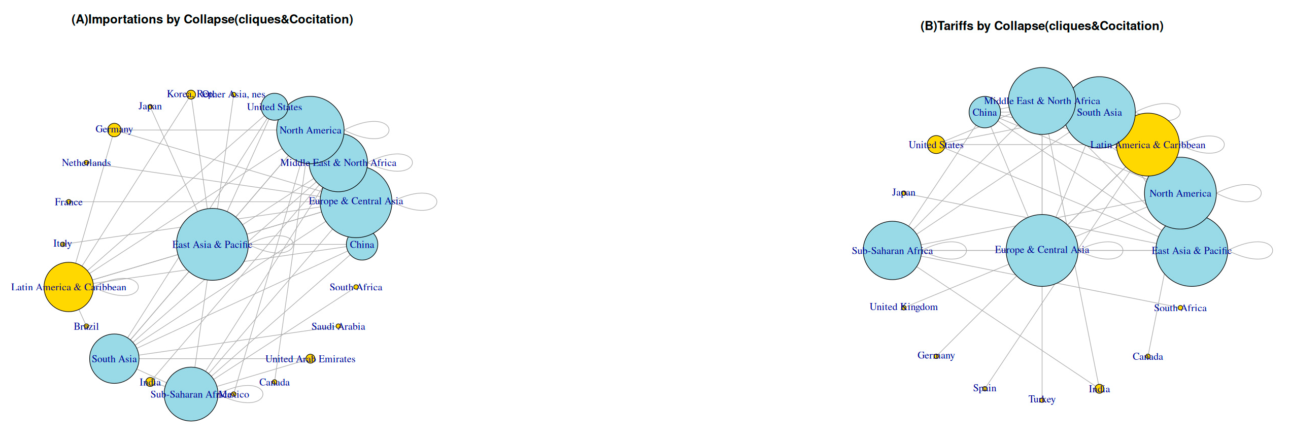
Block B5 has the goal of developing the graph network analysis. Here, the particular characteristic is the creation of the net-igraph object (net_r_Imp or net_r_Tar), which is necessary to communicate the Multi-ERGM network with the “igraph” package for network analysis [69]. This block has several tasks in hierarchical order: (1) Analysis of results from tools like “as_adj_edge_list(net_r)” and “vsize” which are calculated from the degree function; it is possible to calculate the degree density shown in Figure 2 (Section 5, Results). This task is described in the function graph_analysis_n_Imp (or graph_analysis_n_Tar) that has a Multi-ERGM input (n_r_Imp or n_r_Tar) from block B4 and the output is a network type net-igraph object (net_r_Imp or net_r_Tar). (2) Density edge analyses (see Section 5.2) and diameter calculations (see Section 5.3) of the network (net_r_Imp or net_r_Tar), which are shown in Figure 2 and Figure 3; this task is described in the function graph_analysis_2 (more details in Supplementary File S1.1). This function also calculates the frequency of the degrees in histograms as shown in Figures S1–S3 (see Supplementary File S2); from this, task (2) to task (7) do not have outputs. (3) “Hub” analyses (see Section 5.4) of the network (net_r_Imp or net_r_Tar) as shown in Figure 4; this task is described in the function graph_analysis_3. This function also has the “Authority” analyses (see Section 5.5) of the network (net_r_Imp or net_r_Tar) as shown in Figure 5. (4) Distance analysis from the Latin America and Caribbean region to the rest of the vertices involved in the network (net_r_Imp or net_r_Tar) is shown in Figure 6; this task is described in the graph_analysis_4 function. (5) Coupling in co-citation and cliques by mutuality analyses (see Section 5.7) of the network (net_r_Imp or net_r_Tar) are shown in Figure 7, with the coupling in co-citation and cliques by collapse analyses (see Section 5.8) of the network (net_r_Imp or net_r_Tar); these tasks are described in the function graph_analysis_6_1 (for more detail, see Supplementary File S1.1. Pseudo Code by Functions, Function_2.R).

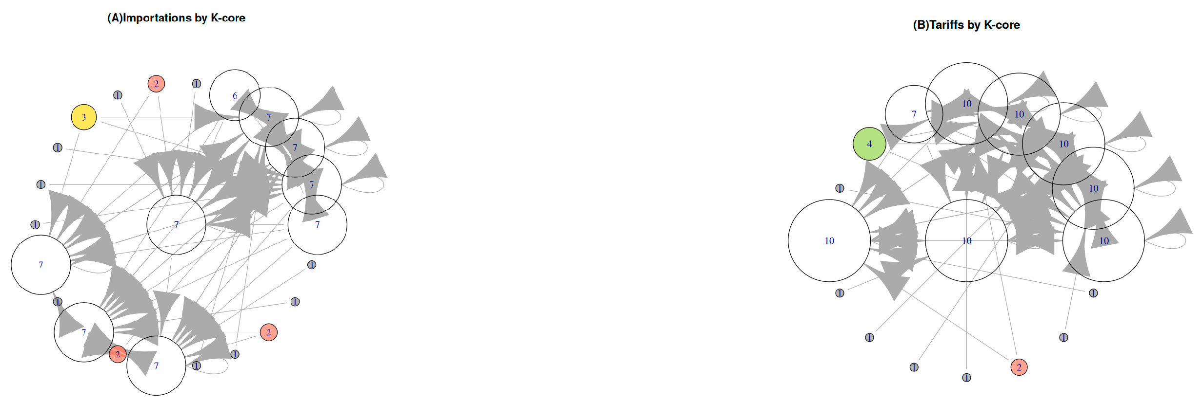
(6) The k-model analyses (see Section 5.9) of the network (net_r_Imp or net_r_Tar) are shown in Figure 8; this task is described in the function graph_analysis_6_0.

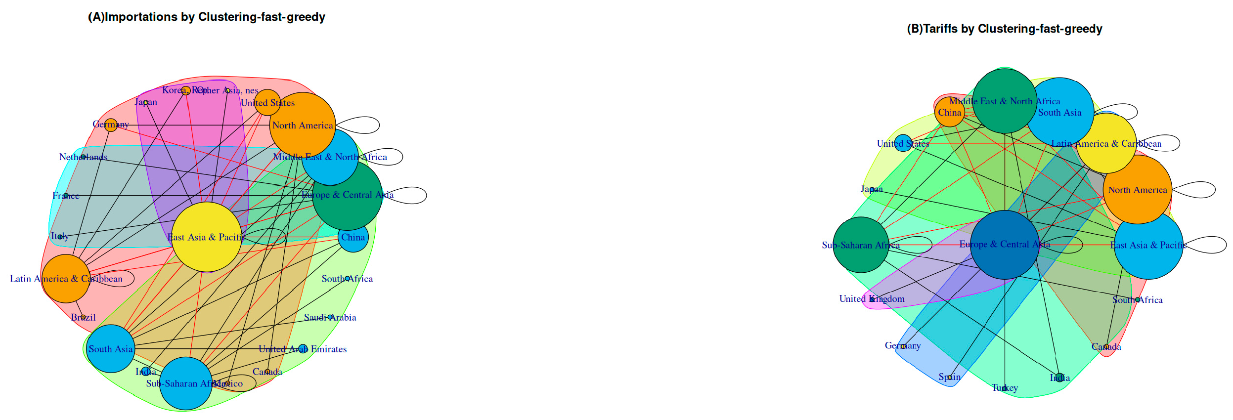
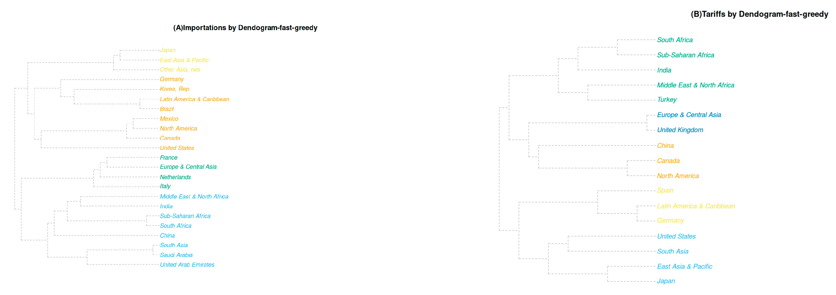
(7) Also, this task is part of the function graph_analysis_6_1 as well, and it is in charge of the community detection by clustering-fast-greedy (see Section 5.10) analysis of the network (net_r_Imp or net_r_Tar), as shown in Figure 9 and Figure 10.

5. Results

5.1. Fundamental Parameter Multi-ERGM Network Analyses

Multi-ERGM RPI Network Analysis: To understand the complex relationship between the actors of this multilayer small network, which corresponds to Multi-ERGM RPI, it is essential to know the total edge density, which is 0.1245059. For more details on how to calculate this parameter, refer to [70]. The reciprocity [45] is calculated with dyad values and the mutuality between the edges, which is 0.2807018. The global transitivity is 0.5030488 and those in specific vertices are as follows: the East Asia and Pacific region with 0.4181818, Europe and Central Asia with 0.3636364, North America with 0.4444444, the Middle East and North Africa with 0.6785714, the LA&CR with 0.4285714, South Asia with 0.5277778, China with 0.8095238, the United States with 0.8666667, and the Republic of Korea, the United Arab Emirates, and India with 1.0000000. The maximum transitivity of Multi-ERGM RPI is 1.0000000 for two elements, and the lowest value is observed in the Europe and Central Asia region.

The betweenness parameters in Multi-ERGM RPI are in the Europe and Central Asia region with 22.0, the East Asia and Pacific region with 39.0, the LA&CR with 6.5, the Middle East and North Africa with 26.0, North America with 23.5, Sub-Saharan Africa with 9.0, South Asia with 10.0, and China, the United States, Japan, Germany, the Netherlands, France, Italy, Brazil, India, Mexico, Canada, the United Arab Emirates, Saudi Arabia, and South Africa with 0.000000. The maximum betweenness is in the East Asia and Pacific region, and the minimum is 10 elements with a value of 0.000000.

Multi-ERGM RPT Network Analysis: A detailed description of the complex Multi-ERGM RPT network requires a meticulous examination to know the total edge density, which is 0.2316176. The reciprocity is calculated with dyad values and the mutuality between the edges, which is 0.6071429. The global transitivity is 0.6375, and those in specific vertices are as follows: East Asia and Pacific, 0.6111111; Europe and Central Asia, 0.6785714; North America, 0.6785714; the Middle East and North Africa, 0.5000000; the LA&CR, 0.4285714; South Asia, 0.7857143; China, 0.9047619; the United States, 0.8333333; Sub-Saharan Africa, 0.5714286; and India, 1.0000000. The maximum transitivity of Multi-ERGM RPT applies to China, and the lowest is that of the LA&CR.

The betweenness parameters in Multi-ERGM RPT are Europe and Central Asia with 10.285714, East Asia and Pacific with 8.976190, North America with 10.285714, the LA&CR with 12.500000, South Asia with 5.119048, the Middle East and North Africa with 9.904762, Sub-Saharan Africa with 7.928571, and China, the United States, Japan, the United Kingdom, Germany, Spain, Turkey, India, Canada, and South Africa with 0.000000. The maximum betweenness is in the LA&CR (LA&CR), and the lowest and the minimum values are 10 elements with a value of 0.000000.

Multi-ERGM RPI vs. Multi-ERGM RPT Analysis: For this comparison, it is fundamental to compare the graph network parameters, like edge density which is 0.1245059 for Multi-ERGM RPI and 0.2316176 for Multi-ERGM RPT with 0.107117 of difference. The reciprocity is 0.2807018 for the first complex network (Multi-ERGM RPI) and 0.6071429 for the second complex network (Multi-ERGM RPT) with 0.3264411 of variation. The global transitivity is 0.5030488 for the first one and 0.6375 for the second one with 0.1344512 of difference. The maximum transitivity of Multi-ERGM RPI is seen for the United Arab Emirates and India and the lowest for the Europe and Central Asian region; alternatively, the maximum transitivity of Multi-ERGM RPT is seen for China and the lowest for the LA&CR. The maximum closeness value (see Note 3) for the first complex network is seen for the Europe and Central Asia region and the lowest for Brazil; in contrast, the maximum closeness value for the second complex network is seen for the East Asia and Pacific region and the lowest value is for Germany. The maximum betweenness for Multi-ERGM RPI is seen for the East Asia and Pacific region, while the maximum betweenness for Multi-ERGM RPT is seen the LA&CR.

Note 3:

In the context of ERGMs multilayer analysis, the weight parameters, such as closeness (centrality based on distance to others in the graph), were configured as follows (see Supplementary File S1.1 and block B5 in pink): closeness(net, mode = “all”, weights = NA).

Partial Conclusions: One of two methods of how to calculate the edge density is as follows (see Supplementary File S1 and methodology block B5 in pink): ecount (net)/(vcount (net) ×vcount (net) −1). That means, the total number of region-partners (see Supplementary File S4. Network list) is involved in the tariff network. The prevalence of ties (cumulative frequency, see Figures S13 and S14 in Supplementary File S4) has 20.8% of the total connectivity over all possible connections in the network, which is higher than the partners from the importation network (12.4%); their connectivity is stronger by 10.7%. The reciprocity parameter helps us to understand the relationship between ties and whether they are reciprocal or mutual. In both multilayer networks, the probability is positive (although it could be negative); the network of tariffs accounts for around a 60% chance of finding a shared partner in reciprocal occurrence compared to the importation partners network. Transitivity is a measure of the presence of triads or triangles (three shared partner groups). Global transitivity indicates that if you randomly select a group of three shared partners in the tariff network, there is a 50.3% chance that they are connected, and in the importation network, a 63.75% chance. Additionally, the maximum transitivity can help us to identify the presence of a specific partner country in the connections of triads.

Possible Diagnosis: One possible reason why the United Arab Emirates and India exhibit the highest transitivity (1.0) in the network of imports (Multi-ERGM RPI) is that these actors have distinct consumer preferences. In an economic context, the transitive preference means they prefer good A over good B. But, in the network analysis, a highly transitive network means the actor A is connected with B, and B with C, and thus A and C are also likely to be connected (due to logistic hubs, strategic geographic location, etc.); a high transitivity also occurs when a country imports goods not for its own use, but to re-export them to other markets, leveraging its position in global market networks. Taking this into account, the United Arab Emirates and India have strong connectivity within the global trade network. In contrast, the Europe and Central Asian region has the lowest transitivity within the global treatment network, as of the last report in 2022.

In the tariff context, the one possible reason why China has the maximum transitivity is due to low average applied tariffs on imported goods and its processing and re-exportation to other countries without paying tariffs or very low tariffs; also, its transitivity is very high (80% of probability) which means their connectivity is very significant in the global treatment. Another possible situation is that the product supply chain, from the raw materials to final product construction, could involve several countries in the process of importations, and concepts like transitivity and edge density (see Section 5) show up referring to how many times (edge density) China is involved on the tariff lists of others countries due to the product supply chain. Instead, the LA&CR has low transitivity (40% of probability) in the tariff network. Actually, historically, the LA&CR has been an exporter of raw materials (see Section 1); as a result, the region lacks the same edge density as China in global treatment and the possibility of government agreements.

5.2. Degree Multi-ERGM Network Analyses

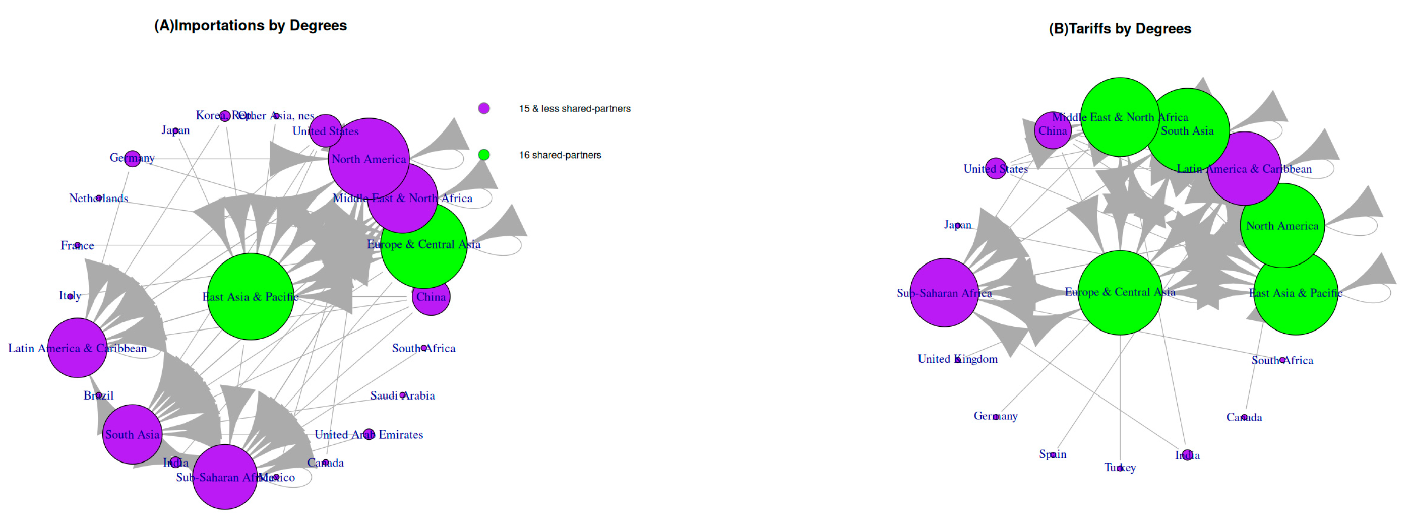
Multi-ERGM RPI Network Analysis: Figure 2A on the left side displays a Multi-ERGM RPI multilayer network, which accounts for a total of 63 edges (see Supplementary File S4. Network lists and Supplementary File S2.2. Edges by vertex.names).

The color classification indicates the vertices and size, with higher numbers of partners represented in green and lower numbers in bright purple. The Multi-ERGM RPI in Figure 2A shows 23 of 63 edges with the highest degree (number of shared partners), which is 16, to the lowest degree, which is 1. In descendant order appear the East Asia and Pacific region and the Europe and Central Asia region with 16 partners (in green); North America with 15; the Middle East and North Africa with 13; Sub-Saharan Africa with 12; the LA&CR and South Asia with 11; China with 7; the United States with 6; Germany with 3; the Republic of Korea, the United Arab Emirates, and India with 2; and Mexico, Italy, Japan, South Africa, Canada, Brazil, the Netherlands, France, and Saudi Arabia with 1 shared partner (see Supplementary File S4.1. Degrees by vertex.names).

Multi-ERGM RPT Network Analysis: Figure 2B illustrates the Multi-ERGM RPT multilayer network, which comprises a total of 63 edges. The color classification displayed, with the number of partners in green and in bright purple, corresponds to the lower vertices/size. The Multi-ERGM RPT (Figure 2B) shows 17 of 63 edges with the highest degree, which is 16, to the lowest degree, which is 1. Europe and Central Asia, East Asia and the Pacific, North America, and South Asia have 16 shared partners (in green); the Middle East and North Africa have 15; the LA&CR has 14; Sub-Saharan Africa has 13; China has 7; the United States has 4; and Japan, the United Kingdom, Germany, Spain, Turkey, Canada, and South Africa have 1 shared partner.

Multi-ERGM RPI vs. Multi-ERGM RPT Analysis: There are considerable differences in degree values, as the Multi-ERGM RPI (Figure 2A) consisted of 23 of 63 edges instead of 17 of the 63 edges from Multi-ERGM RPT (Figure 2B); both complex networks have similarities, with 16 elements having the highest degree values in the Europe and Central Asia region and the East Asia and Pacific region, which are present in both networks, but the Multi-ERGM RPT had differences: North America and South Asia had a degree of 16 as well.

Partial Conclusions: For these analyses, it is essential to note the primary goal of the graph models, namely, the structural analysis of the network. To decode Figure 2, concepts as centrality, betweenness, closeness, etc., are essential because there are nodes that have a bridging function (betweenness) and facilitate communication or connectivity with distant parts of the network. Analyzing the betweenness centrality, for example, we can notice the influence and control (degree values) for a specific node in the network. The maximum betweenness centrality in the importation network corresponds to the East Asia and Pacific region. The closeness parameters provide insight into the importation diameter structure of the network, where the maximum closeness value (0.03125) corresponds to the Europe and Central Asia region, and the lowest is seen for Brazil at 0.01639344. This means Brazil is the most distant node in the structure of the network. The maximum betweenness centrality in the tariff network is seen for Europe and Central Asia, and the closeness parameters give us an idea of the tariff diameter structure of the network because the maximum closeness value (0.04347826) corresponds to the East Asia and Pacific region, and the lowest is seen for Germany (0.02380952).

Possible Diagnosis: One possible reason why the structure of the importation network has a maximum value of betweenness centrality is that the East Asia and Pacific region is involved in 23 of 63 edges in the importations of contemporary global commerce. Their presence in the worldwide commerce has been emerging since the XIX century (see Section 1.2, Section 1.3 and Section 1.4).

In the tariffs context, Europe and Central Asia do not have the maximum betweenness in global commerce importations, but their role is as a land bridge. Historically (see Section 1.1), this region is considered the land with the region’s traditional land routes, such as the Middle Corridor, connecting the major economic centers (maximum closeness corresponds to the East Asia and Pacific region) and providing an alternative to existing treatment flows.

5.3. Diameters and Edges Analyses

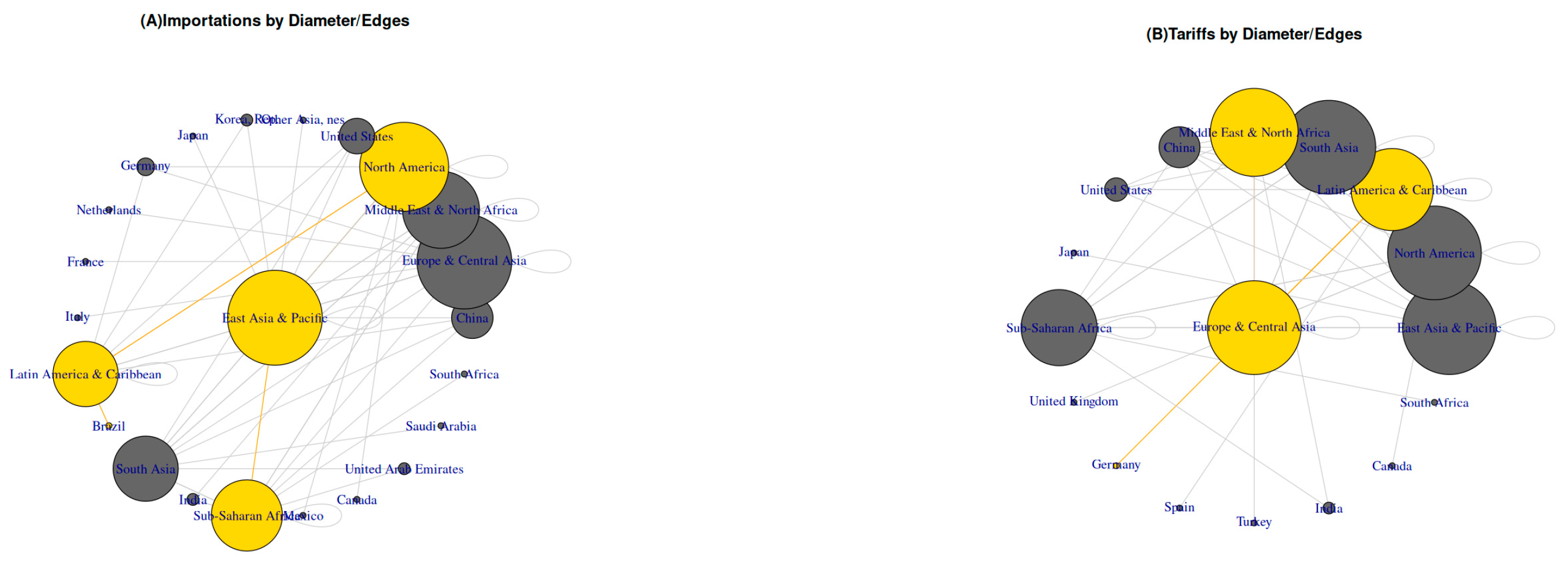
Figure 3 describes the Multi-ERGM diameter and edge analysis, which involves selecting the edges with the highest weight to the lowest weight in the network and choosing the path with the largest connection within the network. This route is described in yellow, and it is known as the vector diameter because it is filled with the names of the edges.

Note 4:

In the context of network structure, weight is the inverse of the node’s average geodesic distance to others in the network, and the ratio of the network is calculated as follows (see Supplementary File S1.1: dyad_census(net)$mut/ecount(net)).

Multi-ERGM RPI vs. Multi-ERGM RPT Analysis: For this comparison, Figure 3 describes the Multi-ERGM RPI (Figure 3A), which shows the largest connection (the largest path in yellow) is between Brazil and the LA&CR to North America, and the shortest path is between the East Asia and Pacific region and Sub-Saharan Africa. Instead, on the left side of Figure 3 (Figure 3B), it describes the Multi-ERGM RPT, the largest path connection is from Germany to Europe and Central Asia to the LA&CR to the Middle East and North Africa. The previous note (see Note 4) makes reference to the transitivity and edge density (dyad_census(net)) in the network by mutuality ($mut) or reciprocal connection divided by the total number of edges in the network.

Partial Conclusions: It is possible to say that the sum of the groups of reciprocity and mutuality sized (weights) is the diameter of the network: (2 × dyad_census(net)$mut/ecount(net)) (see Supplementary File S1.1 and methodology in block B5 in pink). Notably, only the network of importations has the shortest geodesic path (in yellow). However, it is peculiar that in the tariff network the longest path (in yellow) needs to traverse more edges (four-sized nodes in yellow) to create a connection: one node more than the importation’s network.

Possible Diagnosis: One possible reason why the paths (see Figure 3) differ in the importations and tariff networks is due to the mutuality relationship (for more details, see Section 5.7), and the key could be global treatment and government agreements. In that context, it is not surprising that in the tariff network, the longest path and its transitivity are heavier (carry more weight, see Note 4) than in the importation network to reach the last node (diameter of the network): the Middle East and North Africa.

5.4. Hub Multi-ERGM Network Analyses

The hubs and authorities algorithms were developed by Jon Kleinberg [71]. Initially, the application was utilized for studying the structural and morphological aspects of web pages [72]. In this document, we applied hubs and authorities algorithms in the original analysis for Multi-ERGM RPI and Multi-ERGM RPT.

Multi-ERGM RPI Network Analysis: On the left side of Figure 4 (Figure 4A), it describes the Multi-ERGM RPI and shows the hub analysis. This complex multilayer network accounts for the following hub parameters: Europe and Central Asia, East Asia and the Pacific, and China, 1.0000000; the Middle East and North Africa, 0.5754047; North America, 0.8779822; the United States, 0.8779822; the Republic of Korea, 0.2909038; Japan, 0.1455716; Germany, 0.4245953; the Netherlands, 0.1377001; France, 0.1377001; Italy, 0.1377001; the LA&CR, 0.2868952; Brazil, 0.1453322; South Asia, 0.2775051; India, 0.2775051; Sub-Saharan Africa, 0.4298331; Mexico, 0.1415631; Canada, 0.1415631; the United Arab Emirates, 0.2743458; Saudi Arabia, 0.1523280; South Africa, 0.1220178. The maximum Multi-ERGM RPI hub value corresponds to the East Asia and Pacific region and the lowest to South Asia.

Multi-ERGM RPT Network Analysis: On the right side of Figure 4 (Figure 4B), it describes the Multi-ERGM RPT and shows hub analysis. This complex network accounts for the following hub parameters: the Europe and Central Asia region, East Asia and the Pacific, North America, South Asia, and China, 1.0000000; the LA&CR, 0.7256063; the Middle East and North Africa, 0.8688137; the United States, 0.5694961; Japan, 0.1462442; Sub-Saharan Africa, 0.5855364; the United Kingdom, 0.1465716; Germany, 0.1311863; Spain, 0.1311863; Turkey, 0.1370331; India, 0.2743937; Canada, 0.1465716; South Africa, 0.1373606. The maximum Multi-ERGM RPT hub value corresponds to five elements with 1.0000000, and the minimum is Germany.

Multi-ERGM RPI vs. Multi-ERGM RPT Analysis: A designation as a hub in the ERGMs network is a node with a high number of connections as inputs or outputs. This role is fundamental for the flow of interactions in the network. In our analysis, we decided to select the outgoing links. There are several parameters that contribute to the high coefficient of the hub (in green), such as the degree value and the location of the hub within the network, like centrality, betweenness, closeness, etc. The highest value of the coefficient of the hub means the importance of the presence of this node to the network. The multilayer network of importations (Figure 4A) shows South Asia with the minimum hub coefficient value. On the right side of Figure 4, the multilayer network of tariffs (Figure 4B) shows Germany with the minimum hub coefficient value. The maximum coefficients for hubs in Multi-ERGM RPI are for three nodes instead of five hubs, with the highest values in the tariff network.

Possible Diagnosis: Europe and Central Asia, East Asia and the Pacific, and China are the hubs with the maximum flow in importation networks, a well-established fact. The case of South Asia, which appears as the highest hub parameter in the importation network and the lowest in the tariff network, is of particular interest. It is crucial to note that this hub analysis was conducted using the outputs, not the inputs. One possible reason for this is that South Asia is an important center for global sourcing and manufacturing. This region is seen as an alternative to China for manufacturing, making it a strategic geographical player in the worldwide supply chain. However, in the context of the tariff, South Asia is not a major global treatment hub; instead, this region is focused on building trading and global agreements (see Section 1.4, [42]).

Another interesting case is Germany, which appeared as the lowest hub parameter and the lowest closeness in diameter analysis of the tariff network (see Section 5.3).

5.5. Authority Multi-ERGM Network Analyses

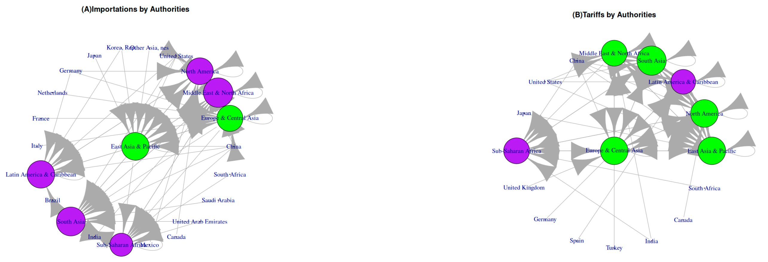
Multi-ERGM RPI Network Analysis: The left side of Figure 5 (Figure 5A) describes the Multi-ERGM RPI, and it shows the authority analysis. This complex network accounts for the following authority parameters: Europe and Central Asia, 0.8856036; East Asia and the Pacific, 0.9362282; North America, 0.9104477; the LA&CR, 0.9346885; the Middle East and North Africa, 1.0000000; South Asia, 0.9796814; and Sub-Saharan Africa, 0.7847443. China, the United States, the Republic of Korea, Japan, Germany, the Netherlands, France, Italy, Brazil, India, Mexico, Canada, the United Arab Emirates, Saudi Arabia, and South Africa have 0.0000000. The maximum Multi-ERGM RPI authority value corresponds to the Middle East and North Africa region, and the minimum is 0.0000000 for 15 network elements.

Multi-ERGM RPT Network Analysis: The right side of Figure 5 (Figure 5B) describes the Multi-ERGM RPT, and it shows the authorities analysis. This complex network accounts for the following authority parameters: Europe and Central Asia, 0.9454252; East Asia and the Pacific, 0.9433131; North America, 0.9454252; the LA&CR, 0.8461856; South Asia, 1.0000000; the Middle East and North Africa, 0.8838994; and Sub-Saharan Africa, 0.8860116. China, the United States, Japan, the United Kingdom, Germany, Spain, Turkey, India, Canada, and South Africa have 0.0000000. The maximum Multi-ERGM RPT authority value corresponds to South Asia, and the minimum is 0.0000000 for 10 network elements.

Multi-ERGM RPI vs. Multi-ERGM RPT Analysis: The maximum coefficient of authorities in the Multi-ERGM RPI multilayer network corresponds to the Middle East and North Africa region instead of South Asia, which has the coefficient of authorities in Multi-ERGM RPT; in comparison with the minimum value of authorities in Multi-ERGM RPI (Figure 5A), there are 15 network elements instead of 10 network elements with the minimum values of authorities in Multi-ERGM RPT (Figure 5B).

Partial Conclusions: In contrast to the hubs, the authorities in the complex multilayer networks have the peculiar characteristic of being an authority in the hierarchical structure of the network. Usually, these nodes have a large number of incoming connections. This is another difference from the hubs because the hubs have inputs or outputs, having the flow or control of the connectivity, like a bridging configuration. In the comparison between the networks, the authority in the importation network corresponds to the Middle East and North Africa region, with the maximum number of inputs, instead of South Asia, with the authority in the tariff network.

Possible Diagnosis: One possible reason why South Asia appears with the highest number in the authority parameter in the tariff network and in the hub’s context (see Section 5.5) is that South Asia is not a major global treatment hub; this is the mutuality concept. In Multi-ERGMs RPT, South Asia had a value of 0.7857143, very similar to China with 0.9047619 and the United States with 0.8333333. In the network structure context, an authority score measures the value of a node’s own content which is pointed to by many good hub nodes.

5.6. Distances Multi-ERGM Network Analyses

The previous comparative analyses (Section 5.1, Section 5.2, Section 5.3, Section 5.4 and Section 5.5) and the next ones (Section 5.7, Section 5.8, Section 5.9 and Section 5.10) were developed from a global perspective, and this analysis section describes the particular case of the LA&CR, detecting the vertex v_LA<-V(net)$name == “Latin America and Caribbean” (see function graph_analysis_4 at block B5 in pink) and starting a series of analysis.

Multi-ERGM RPI Network Analysis: The Multi-ERGM RPI distances from the LA&CR to the rest of the elements are shown in Figure 6 on the left side (Figure 6A); to itself it is zero, and it is in blue. South Africa, the United Arab Emirates, Saudi Arabia, and India are the largest distances of three in bright yellow; the distances to the Middle East and North Africa, Japan, the Netherlands, France, Italy, South Asia, Sub-Saharan Africa, Mexico, and Canada are two and are in dark yellow; East Asia and the Pacific, China, Europe and Central Asia, North America, the United States, the Republic of Korea, Germany, and Brazil are the minimum distance of one in dark purple.

Multi-ERGM RPT Network Analysis: The Multi-ERGM RPT distances from the LA&CR to the rest of the elements are shown in Figure 6 on the right side (Figure 6B); to itself it is zero, and it is in blue. Turkey, South Africa, and India are the most extensive distances of three in bright yellow; the Middle East and North Africa, Japan, Sub-Saharan Africa, and the United Kingdom are two in dark yellow; Europe and Central Asia, East Asia and the Pacific, North America, South Asia, China, the United States, Germany, and Spain are the minimum distance of one in dark purple.

Multi-ERGM RPI vs. Multi-ERGM RPT Analysis: The distance models can be configured with the following options: Johnson, Bellman–Ford, Dijkstra, Floyd–Warshall, unweighted, and automatic [73]; in this case, the unweighted and automatic options are used (Figure 6). The minimum distances from the LA&CR to the rest of the elements are shared in both complex networks (6): Europe and Central Asia, East Asia and the Pacific, North America, China, the United States, and Germany. On the other hand, the Republic of Korea and Brazil also appear as having minimum distances from the LA&CR in Multi-ERGM RPI instead of East Asia and the Pacific, South Asia, and Spain in Multi-ERGM RPT (Figure 6B).

Partial Conclusions: In the context of network structure and graph theory, the statistical distance is defined as the shortest path and can be calculated using different algorithms. In this case, the selection of the vertex is based on the node match, and from this node, the distance is calculated using the unweighted Hamming distance and considering neighboring edges, triangles, population size, etc. It is essential to note the differences from the Bellman–Ford method, which considers negative edge weights, and the Johnson algorithm, which is based on Euclidean spaces, among others.

Possible Diagnosis: In the importation network with the biggest actors of global commerce, such as East Asia and the Pacific, China, and Europe and Central Asia, it is not a surprise to have the nearest distance with them. And comparing these results with the clustering-fast-greedy (see Section 5.10 for more details), it results that the LA&CR is part of Community 2 (which has eight actors), as well as North America, the United States, the Republic of Korea, and Germany.

In the tariffs context, the biggest actors of global trade commerce are Europe and Central Asia, East Asia and the Pacific, North America, South Asia, China, and the United States. And comparing these results with the clustering-fast-greedy (see Section 5.10 for more details), Community 4 has three actors: the LA&CR, Germany, and Spain.

5.7. Co-Citation and Cliques by Mutual Analysis

Figure 7 and Figure 11 were generated using the co-citation and cliques algorithm. The coupling in co-citation is an algorithm that identifies two vertices as co-cited if there is another vertex that co-cites both of them, and they are selected [69]. The result is a count of how many types of two vertices are co-cited. Before proceeding with this analysis, it is essential to verify that the network contains elements with undirected relationships between them. There are three configurations of undirected networks: mutual, collapse, and by each one. We worked with the mutual and collapse options (see graph_analysis_6_1 at block B5 in pink). This section starts with the mutual dyad or reciprocity subsets.

This function is part of the “igraph” packages [69], and its theoretical basis is derived from the Bron–Kerbosch algorithm and is described in detail in the document “Listing All Maximal Cliques in Sparse Graphs in Near-Optimal Time” by David Eppstein et al. [74]. This algorithm identifies all complete subgraphs within the given graph. The input graph, despite being directed, will be processed as undirected; any duplicate edges or loops will be disregarded. If the graph is missing a weight vertex attribute and the argument is set to NULL, every vertex will be assigned a weight of 1. It is important to note that the current implementation of the weighted clique finder only supports a positive whole number weight, which, in this instance, is 1.

Multi-ERGM RPI Network Analysis: On the left side of Figure 7 (Figure 7A), in Multi-ERGM RPI, the co-citation and cliques are shown in mutual analysis. The most extensive cliques with the maximum number of nodes are in blue, and the remaining cliques are yellow. Figure 7A describes the Multi-ERGM RPI matrix result of co-citation, which accounts for a total of 529 elements co-cited by 2 vertices with 23 vertices in total. The list of n clique elements in the mutual analysis is 33, where the maximum size of cliques is 3/23 vertices and the minimum is 1/23 vertices. The most extensive cliques are the two with the maximum number of nodes: (1) Element 27 with 3/23 vertices is the Middle East and North Africa → South Asia → Sub-Saharan Africa (in light blue); (2) Element 31 with 3/23 vertices is East Asia and the Pacific → Europe and Central Asia → North America (in light blue).

Multi-ERGM RPT Network Analysis: On the right side of Figure 7 (Figure 7B), in Multi-ERGM RPT, the co-citation and cliques are shown in mutual analysis. Figure 7B describes the Multi-ERGM RPT (Figure 7B) matrix result of co-citation, which accounts for a total of 289 elements co-cited by 2 vertices with 17 vertices in total. The list of n clique elements in the mutual analysis is 65, where the maximum size of cliques is 5/17 vertices and the minimum is 1/17 vertices. The most extensive cliques are the two with the maximum number of nodes: (1) Element 54 with 5/17 vertices are Europe and Central Asia → East Asia and the Pacific → North America →the LA&CR → South Asia (in light blue); (2) Element 38 with 5/17 vertices is Europe and Central Asia → East Asia and the Pacific → North America → South Asia → the Middle East and North Africa (in light blue).

Multi-ERGM RPI vs. Multi-ERGM RPT Analysis: We are looking for the most extensive clique by degeneracy (a frequently used measure of the sparseness of a graph) which is closely related to other standard sparsity measures such as arbocity and thickness [74]. The co-citation Multi-ERGM RPI matrix in mutual analysis consisted of 529 elements by 23 vertices in total. Additionally, it identified 33 cliques, and their most extensive cliques have 3/23 elements. Instead of 289 elements by 17 vertices from the co-citation algorithm of the Multi-ERGM RPT multilayer network, there are 65 cliques, of which the most extensive cliques have 5/17 elements.

Partial Conclusions: The network of importations has more elements co-cited in mutual relationships or in sparsity. This network has around twice as many dyads in comparison with the tariff network. If the co-citation algorithm identifies similarities between nodes and, in this case, a mutual relationship, it could indicate that the network of importations is more cohesive.

Possible Diagnosis: The Middle East and North Africa, South Asia, and Sub-Saharan Africa clique, one of the largest in the importation network, is significant due to its shared historical mutual commerce activity (see Section 1.1). This historical activity could play a crucial role in shaping this clique. The second-largest cliques in the importation network are East Asia and the Pacific, Europe and Central Asia, and North America. They also share mutually dense edges in global commerce, as well as in the context of tariffs. However, the LA&CR, part of one of the largest cliques in the tariff network, is a unique case. Their position could be due to their distinct historical trade and agreements (see Section 1.2).

5.8. Co-Citation and Cliques by Collapse Analysis

Multi-ERGM RPI Network Analysis: The co-cited matrix is the same for Figure 7 and Figure 11. That means, Figure 11A describes the Multi-ERGM RPI matrix result of co-citation, which accounts for a total of 529 elements co-cited by 2 vertices with 23 vertices in total. The Multi-ERGM RPI’s list of cliques in collapse has 191 elements, where the maximum size of cliques is 6/23 vertices and the minimum is 1/23 vertices. The most extensive cliques are three: (1) Element 101 with 6/23 vertices is East Asia and the Pacific → Europe and Central Asia → the Middle East and North Africa → North America → the United States → South Asia (in light blue); (2) Element 141 with 6/23 vertices is East Asia and the Pacific → China → the Middle East and North Africa → South Asia → Sub-Saharan Africa (in light blue); (3) Element 143 with 6/23 vertices is East Asia and the Pacific → China → Europe and Central Asia → the Middle East and North Africa → North America → South Asia (in light blue).

Multi-ERGM RPT Network Analysis: On the right side of Figure 11 (Figure 11B), in the Multi-ERGM RPT, the co-citation and cliques are displayed in the collapse analysis. The co-cited matrix is the same for mutual and collapse analysis (Figure 7 and Figure 11). Figure 11B describes the Multi-ERGM RPT matrix result of co-citation, which accounts for a total of 289 elements co-cited by 2 vertices with 17 vertices in total. The Multi-ERGM RPT’s list of cliques in collapse has 189 elements, where the maximum size of cliques is 7/17 vertices and the minimum is 1/17 vertices. The most extensive clique is one with 7 vertices: Element 115 with 7/17 vertices are Sub-Saharan Africa→ Europe and Central Asia →China → the Middle East and North Africa→ South Asia→ North America→ East Asia and the Pacific (in light blue).

Multi-ERGM RPI vs. Multi-ERGM RPT Analysis: In a previous analysis by mutuality (reciprocity), from the Multi-ERGM RPI multilayer network, 33 cliques with 3/23 elements were found. Here, the Multi-ERGM RPI network by the collapse configuration consisted of 191 cliques with a maximum number of elements of 6/23. In the previous analysis by mutuality, the Multi-ERGM RPT multilayer network consisted of 65 cliques, of which the most extensive clique had 5 out of 17 (5/17) elements. Here, the Multi-ERGM RPT network using the collapse configuration consisted of 189 elements, where the maximum size of cliques is 7/17.

Partial Conclusions: Analyzing the multilayer network of importations, both methods (mutual and collapse) provide clues on how the cliques share country partners. In the collapse technique, 191 subsets are approximately five-times larger than the cliques using mutual relationships. In the collapse technique, the subsets are in co-citation under any attribute. Additionally, in the multilayer network of tariffs, the cliques using collapse are more numerous than those using mutual relationships, which is comprehensible, as they are around three-times more numerous than cliques using mutual relationships.

Possible Diagnosis: One reason why the cliques in the collapse technique co-cited more than in mutuality is due to any commerce activity detected in the tariff context or without tariffs, by any good importation in a group. This method creates a print of this relationship. It is not necessary for a historical commercial relation to exist if a co-citation occurs; it establishes a clique, with or without mutuality.

5.9. K-Model

In 2003, Vladimir Batageli and Matjaz Zaversnik, in their work “An O (m) Algorithm for Cores Decomposition of Networks”, talked about the structure of dense networks and how to partition them into smaller parts, into cohesive subgroups of actors among whom there are strong, direct, intense, frequent, or positive ties. Several publications work on formal descriptions of cohesive groups: n-cliques, n-clans, n-clubs, k-plexes, k-cores, lambda sets, etc. This section describes the implementation of the k-core decomposition (see graph_analysis_6_0 at block B5 in pink).

Figure 8 illustrates, on the left side (Figure 8A), the coreness analysis of the Multi-ERGM RPI, and on the right side (Figure 8B), the Multi-ERGM RPT. This figure shows the application of K-core decomposition, where every vertex represents its degree K value and its interaction within this network, as indicated by imports in 2022. In bright purple appears the lowest K value of 1 degree, in pink the K of 2, in yellow the K of 3, in light green the K of 4, and in white the K ≥ 6.

Multi-ERGM RPI Network Analysis: On the left side of Figure 8 (Figure 8A), it describes Multi-ERGM RPI, with the highest K values (eight) for the East Asia and Pacific region, China, Europe and Central Asia, the Middle East and North Africa, North America, the LA&CR, South Asia, and Sub-Saharan Africa with K values of seven; the United States has a K value of six, Germany has a K value of three, the Republic of Korea, India, and the United Arab Emirates have K values of two; Other Asia, NES (Note 5), Japan, the Netherlands, France, Italy, Brazil, Mexico, Canada, Saudi Arabia, and South Africa (ten) have K values of one.

Note 5:

In Other Asia, NES (Not Elsewhere Specified) is designed using the United Nations Comtrade and often serves as a proxy for Taiwan in trade statistics.

Multi-ERGM RPT Network Analysis: On the right side of Figure 8 (Figure 8B), in Multi-ERGM RPT, the highest K values (seven) are seen for Europe and Central Asia, the East Asia and Pacific region, North America, the LA&CR, South Asia, the Middle East and North Africa region, and Sub-Saharan Africa with K values of 10; China has a K value of 7; the United States, 4; India, 2; and Japan, the United Kingdom, Germany, Spain, Turkey, Canada, and South Africa (seven) have K values of 1.

Multi-ERGM RPI vs. Multi-ERGM RPT Analysis: As a result, in the base with the highest K values of Multi-ERGM RPI were eight elements with value 7, in contrast to the highest K values of Multi-ERGM RPT which were seven elements with value 10. The elements shared were the East Asia and Pacific region, Europe and Central Asia, the Middle East and North Africa region, North America, the LA&CR, South Asia, and Sub-Saharan Africa, except China, which appears only in the Multi-ERGM RPI (Figure 8).

Partial Conclusions: The advantage of this graph analysis lies in the hierarchical identification of nodes based on degrees and density in dense networks. It is essential to imagine and embed cores, where its maximum core, called the main core, has embedded (or nested) n number of vertices. This improvement was analyzed in 2003 by the authors Batageli and Zaversnik in their publication. The higher K value indicates a higher density of connections to subsets of subgroups within the core of the network, as determined by coreness analysis. The density can be sized using the sorting of the neighboring vertices in increasing order of their degrees using bin-sort. The degrees can be in-degree, out-degree, or all. In this case, we worked with “all” options (in-degree and out-degree). Due to the neat work of k-core identification, it is very clear that the graph differences between importations and tariffs are in the multilayer networks. The tariff networks have more dense subsets and a higher hierarchical value than the importation networks.

Possible Diagnosis: Comparing the highest K values (with the highest value 7) and density edges (the highest values from 7 to 16), both in importation networks, they display the same actors: the East Asia and Pacific region, Europe and Central Asia, the Middle East and North Africa region, North America, Sub-Saharan Africa, the LA&CR, South Asia, and China.

Comparing the highest K values (with the highest value 10) and density edges (the highest values from 7 to 16), both in tariff networks, they display similar actors: Europe and Central Asia, the East Asia and Pacific region, North America, South Asia, the Middle East and North Africa, the LA&CR, and Sub-Saharan Africa.

It is interesting that China appears in the highest classification of K in importations but not in the tariff network. In the context of tariffs, in both methods (K-model and density degree), China’s is the highest K value, at 10, but it is very close to 7. These results are similar to those from Section 5.4 and Section 5.5.

5.10. Clustering

In 2004, Mark Newman proposed the fast-greedy algorithm, which has a time complexity of O (n2) for sparse networks. In the same year, Clauset, Newman, and More improved the algorithm, achieving identical results with lower computational resources consumed. The fast-greedy algorithm executes CNM (Clauset–Newman–More) to identify groups of nodes that are more densely connected within themselves. The fast-greedy algorithm iteratively merges communities to maximize a modularity measure, which quantifies the quality of the community structure in terms of centrality, edge betweenness, membership, bridges, likelihood classification, and other factors. It employs the randomized greedy approach to determine core groups, utilizing these core groups as an initial partition for the randomized greedy method to identify community structure and maximize modularity. This method was described in 2009 by Biao Xiang, En-Hong Chen, and Tao Zhou in their research.

Figure 9 illustrates community detection using the CNM (Clauset–Newman–More) algorithm, which clusters partners that share the same particularities, such as merges and edge weights. These attributes are incorporated into the community detection model, which was implemented using fast-greedy modularity optimization to find community structure based on the modularity score. Figure 9 was grouped into clusters using graph polygons in different colors.

Multi-ERGM RPI Network Analysis: As a result of this analysis, in Figure 9 on the left side (Figure 9A), it describes the CNM. It shows four clusters into Multi-ERGM RPI: Community 1 (eight vertices)—North America, the United States, the Republic of Korea, Germany, the LA&CR, Brazil, Mexico, and Canada (cluster in red); Community 2 (eight vertices)—China, the Middle East and North Africa, South Asia, India, Sub-Saharan Africa, the United Arab Emirates, Saudi Arabia, and South Africa (cluster in light green); Community 3 (four vertices)—the Europe and Central Asia region, the Netherlands, France, and Italy (cluster in light blue); Community 4 (two vertices)—the East Asia and Pacific region and Japan (cluster in light purple). Additionally, Figure 9A displays the Multi-ERGM RPI network, which shows the five communities detected: in orange, Community 1 (eight vertices); in blue, Community 2 (eight vertices); in yellow, Community 3 (four vertices); and in green, Community 4 (two vertices).

Multi-ERGM RPT Network Analysis: In Figure 9 on the right side (Figure 9B), the CNM found five clusters into Multi-ERGM RPT: Community 1 (three vertices)—Canada, China, and North America (cluster in red); Community 2 (four vertices)—East Asia and the Pacific, South Asia, the United States, and Japan (cluster in yellow); Community 3 (five vertices)—the Middle East and North Africa, Sub-Saharan Africa, Turkey, India, and South Africa (cluster in light green); Community 4 (three vertices)—the LA&CR, Germany, and Spain (cluster in light blue); Community 5 (two vertices)—Europe and Central Asia and the United Kingdom (cluster in light purple). Likewise, Figure 9B complements this analysis by splitting the cluster elements using a dendrogram with the five communities detected; this dendrogram of Multi-ERGM RPT shows the five communities detected: in orange, Community 1 (three vertices); in light blue, Community 2 (four vertices); in green, Community 3 (five vertices); in yellow, Community 4 (three vertices); and in blue, Community 5 (two vertices).

Multi-ERGM RPI vs. Multi-ERGM RPT Analysis: The Clauset–Newman–More algorithm, using fast-greedy, identified four communities that share characteristics, clustering into graphical polygons in Multi-ERGM RPI, as opposed to the five clusters identified in Multi-ERGM RPT. In both clusters, red shared partners include Canada and the North America region. However, in Multi-ERGM RPI, the United States, the Republic of Korea, Germany, the LA&CR, Brazil, and Mexico are listed, whereas China is absent in Multi-ERGM RPT. Clusters in light green in both cases shared partners, including the Middle East and North Africa, Sub-Saharan Africa, India, and South Africa. In contrast, Multi-ERGM RPI includes China, South Asia, the United Arab Emirates, and Saudi Arabia, whereas Multi-ERGM RPT includes Turkey. Clusters in light blue and light purple do not appear as having any shared partners. Multi-ERGM RPT has an additional cluster in yellow, which includes East Asia and the Pacific, South Asia, the United States, and Japan (Figure 9).

Partial Conclusions: The complementary information to the clustering (Figure 9) of the dendrograms (Figure 10) is interesting, because it is possible to see deeply the hierarchical structure of each clustering, as in the importation network where Community 1 (in orange) actors like the LA&CR have the same hierarchical level as Brazil, Mexico and the North America region; but the United States has the higher hierarchical level in the same cluster. Comparing the tariff network, the actors are in other clusters; however, the case of the LA&CR has the lowest level of hierarchy, as does Germany, from Community 4 (in yellow). In contrast, Spain has the highest level within this cluster.

Possible Diagnosis: Analyzing importation community detection, it is interesting that for the biggest clusters (Community 2, Community 3, and Community 4), it appears that geographical location is the key factor. For Community 2, the group consists of eight actors: China, the Middle East and North Africa, South Asia, India, Sub-Saharan Africa, the United Arab Emirates, Saudi Arabia, and South Africa. Community 3 (four actors) consists of the Europe and Central Asia region, the Netherlands, France, and Italy. In addition, Community 4 (two actors) comprises the East Asia and Pacific region and Japan (this actor has a lot of influence in the commerce of the 19th century, see Section 1.2).

The results are interesting for the other biggest cluster (Community 1), with it appearing that the geographical factor is what joins this group of eight actors as well: North America, the United States, the LA&CR, Brazil, Mexico, and Canada. However, seeing the Republic of Korea and Germany in this group, one possible reason is the manufacturing sector, particularly the automotive industry, where the most significant German partners in the LA&CR are Brazil, Mexico, Chile, and Argentina, as well the Republic of Korea (see Commerce in the XXI Century, Section 1).

In the tariff context, the clustering change is due to historical trade patterns, government agreements, business-friendly trade policies, and tariff-free zones, among other factors. In this case, it is interesting to see the LA&CR in Community 4 (three actors) joining the group with Germany and Spain (due to the historical relationship with this actor, see Section 1).

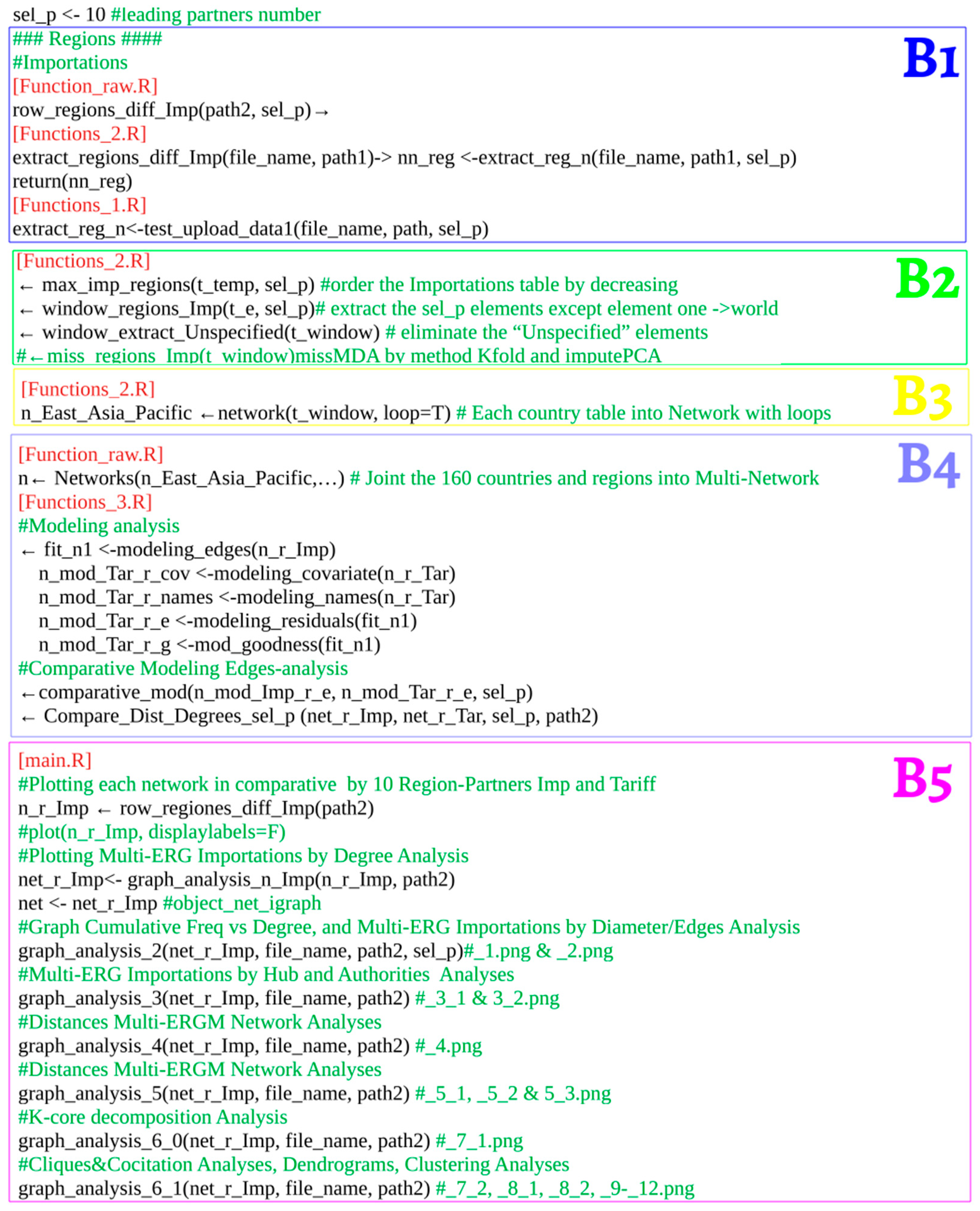
6. Conclusions

This research endeavors to apply static and small exponential random graph models within the context of complex multilayer networks. The proposed methodology constitutes a significant contribution, offering a meticulously detailed, five-block (Bn) procedural framework, complemented by the Supplementary Materials that furnish essential notes to facilitate the replication and verification of the presented approach. These core blocks are systematically organized into five distinct sections, as illustrated in Figure 2, wherein each section is structured to encompass a hierarchical arrangement of tasks and sub-tasks, ensuring a clear and logical progression throughout the analytical process. The most demanding aspects of this work concentrate on the intricacies of model construction, which is further detailed in Section 4, and the strategic selection of a representative sample, denoted as (sel_p). Furthermore, Section 4 serves as the foundational framework, laying the groundwork necessary for effectively addressing and resolving the thought-provoking research questions initially articulated and established in the Hypotheses Section (refer to Section 3).

Hypothesis 1 investigates the application of small network analysis to the realm of global trade, with a specific focus on facilitating a comparative study between tariff structures and importations, as articulated in Hypothesis 2. In this comparative approach, the initial and crucial step involves constructing and observing the convergence patterns of the parameters within the models (eight); these models and their graphical visualizations are detailed and elucidated in Figure S4. The analysis demonstrates that both the Multi-ERGM RPI and Multi-ERGM RPT models exhibit convergence at the same value of eight. The detailed sensitive model specification is presented in Table S1, and a thorough explanation and contextualization of this specification can be found in block B2. The comparative analysis of the convergence characteristics, encompassing both the models themselves and their corresponding graphical representations (incorporating the estimated fitted value edges), reveals that due to the same characteristics between Multi-ERGM RPI and Multi-ERGM RPT networks, they can be comparable.

The examination of the historical connections among the diverse network actors was interlinked and described in detail in Section 5, specifically within the Partial Conclusion Sections, with an initial reference also made in Section 1 to establish foundational context. This core concept, pertaining to the interconnectedness of these actors, was formally posited and subsequently substantiated within Hypothesis 3, which serves as a crucial contextual backdrop for the overall research endeavor. The multifaceted perspectives and in-depth analyses presented across Section 5, ranging from Section 5.1 to Section 5.10, provide substantial empirical perspectives that support the fundamental notion that each algorithm possesses a distinct and intrinsic essence. Furthermore, the acquisition and application of detailed knowledge regarding the operational mechanisms of these algorithms demonstrably facilitate the generation of profoundly insightful and impactful results. This assertion is supported by a thorough examination of the concise summaries derived from the individual subsections (specifically referencing the comparative analysis between Multi-ERGM RPI vs. Multi-ERGM RPT analysis), which were presented and thoroughly discussed during the dedicated discussion sessions (as indicated by references to Partial Conclusions and Possible Diagnosis). The results of these summaries, in particular, demonstrate an impressive level of both adequacy and precision in their representation of the complex actor roles in analytical findings.

The investigation into the LA&CR, conducted within Section 5, placed significant emphasis on detailed analysis of the various distances present within the network, a visual representation of which is further elucidated in Figure 6. A key aspect of this analytical phase centered on a comparative examination, explicitly focusing on the critical vertex v_LA and its relationship to all other constituent elements that are an integral part of the network. This comparative analysis was explicitly designed to directly address and provide empirical support for Hypothesis 4, which was a central tenet of our research framework.

It is particularly noteworthy that, throughout the entirety of this research endeavor, all four initially proposed hypotheses were not only successfully substantiated but also provided strong and consistent evidence for their validity.

Beyond the primary focus on hypothesis testing, the investigation also proved to be instrumental in facilitating the identification of distinct and nuanced angles or perspectives within the information landscape (degree analyses, diameter and edges analyses, hubs and authority analyses, co-citation and cliques in mutual and in collapse approaches, k-core decomposition analyses, and clustering analyses).

These six angles in the big picture represent specific areas where each actor, or entity within the network, demonstrates a heightened and discernible level of content knowledge or expertise. Consequently, the current document holds significant potential to delve more deeply into these precisely identified areas of interest. A key focus of this exploration will be on examining and thoroughly exploring the peaks, representing maximum levels of activity or information, and the troughs, signifying minimum levels, that are observed within the behavioral patterns of each actor.

In our case, the degeneracy of the model is going to occur in values sel_p >> 10, referred to in the Section Multi-ERGMs Sensitive-Model Specifications. If degeneracy occurs, meaning the model inadequately represents the observed network, the simulated networks generated by the MCMC chains may diverge significantly, thus impacting the estimation. In the most extreme cases, the simulated networks could be so dissimilar that the algorithm fails. This implies the specified model would not have produced the observed network. Consequently, in such instances, it is impossible to derive coefficient estimates; therefore, the GOF function cannot be used to analyze discrepancies between model simulations and the observed data. Nevertheless, MCMC diagnostics can still be employed to monitor the performance of the simulation algorithm. The first study to discuss this issue in-depth was Handcock’s in 2003. Subsequently, the model degeneracy within the ERGMs network was described by Snijders and colleagues in 2006 in their publication, and the most recent study was developed by Schweinberger in 2011.

Future Work

Making a wrap-up of the Section Selection of the Region-Partners Dataset and Figure S12 (Supplementary File S3. Saturated Figures), this task was defined for countries’ analyses. The countries’ analyses had homologous blocks (Bn) of regions/countries as row_countries_diff_Imp or row_countries_diff_Tar (see Function_1.R in Supplementary File S1). This section summarizes that the dataset regions/countries is the best option for this application, but for managing a small network of countries’ analyses, it is cost-effective. The graphical method indicates that it is necessary to move to the large network (“bigergm” packages) and to us statistics (“hergm” packages). This concept was previously investigated by Martínez Dahbura and colleagues in 2021, and more recently by Fritz and colleagues in 2024. Consideration of this approach is recommended for future research, in comparison with the current document.

Given the nature of the data [67], and the degeneracy of the model, can a generalized model be developed? Would this model remain effective in the event of data alterations? The following considerations are proposed:

(1) Implement data pertaining to specific products or goods, such as raw materials or manufactured goods, instead of the data of all products (refer to B2, Section 4.1.2).

(2) Modify the current data of the coin, instead of $Import.US.Thousand, to select a specific region, to analyze the quantity of imports per year, and to analyze the conversion or movements of continuous trade values in comparison with USD.

References

1. Bértola, L. Institutions and the Historical Roots of Latin American Divergence. In The Oxford Handbook of Latin American Economics; Oxford University Press: Oxford, UK, 2011; p. 26. [Google Scholar] [CrossRef]
2. Furtado, C. Economic Development of Latin America: Historical Background and Contemporary Problems (No. 8); Cambridge University Press: Cambridge, UK, 1976. [Google Scholar] [CrossRef]
3. Engerman, S.L.; Sokoloff, K.L. Colonialism, inequality, and long-run paths of development. In NBER Working Paper Series; No. 11057; National Bureau of Economic Research: Cambridge, MA, USA, 2005. [Google Scholar] [CrossRef]
4. Acemoglu, D.; Johnson, S.; Robinson, J.A. The colonial origins of comparative development: An empirical investigation: Reply. Am. Econ. Rev. 2012, 102, 3077–3110. [Google Scholar] [CrossRef]
5. Jung, S.; Thomas, L.M. (Eds.) Edges of Transatlantic Commerce in the Long Eighteenth Century; Routledge: Abingdon, UK, 2021. [Google Scholar] [CrossRef]
6. Coffman, D.M.; Leonard, A.; O’Reilly, W. The Atlantic World; Routledge: New York, NY, USA, 2015. [Google Scholar]
7. Bailyn, B. The idea of Atlantic history. Itinerario 1996, 20, 19–44. [Google Scholar] [CrossRef]
8. Gilroy, P. The Black Atlantic: Modernity and Double Consciousness; Harvard UP: Cambridge, MA, USA, 1993. [Google Scholar]
9. Smith, A. An Inquiry into the Nature and Causes of the Wealth of Nations; Strahan, W., Cadell, T., Eds.; William Strahan and Thomas Cadell: London, UK, 1776; Volume 1. [Google Scholar]
10. Kaller, M.; Jacob, F. (Eds.) Transatlantic Trade and Global Cultural Transfers Since 1492: More than Commodities; Routledge: London, UK, 2019. [Google Scholar] [CrossRef]
11. Barnett-Woods, V. Pirates, Slaves, and Profligate Rogues: Sailors of Color in the Eighteenth-Century Maritime World. In Edges of Transatlantic Commerce in the Long Eighteenth Century; Routledge: London, UK, 2021; pp. 18–45. [Google Scholar] [CrossRef]
12. Williams, H.M. Peru, a poem. New Univers. Mag. Or Misc. Hist. Philos. Political Polite Lit. 1784, 75, 203–207. [Google Scholar]
13. Thomas, L.M. “Peruvia’s Bleeding Land”: Bodyscape Commerce in Helen Maria Williams’s Peru. In Edges of Transatlantic Commerce in the Long Eighteenth Century; Routledge: London, UK, 2021; pp. 74–103. [Google Scholar] [CrossRef]
14. Sánchez, J. Helen Maria Williams’s Peru and the Spanish Legacy of the British Empire. In Romanticism’s Debatable Lands; Palgrave Macmillan: London, UK, 2007; pp. 172–185. [Google Scholar] [CrossRef]
15. Goergen, C. A Cure, Both for Soul and Body: “Transculturation in Robinson Crusoe’s Tobacco” Application. In Edges of Transatlantic Commerce in the Long Eighteenth Century; Routledge: London, UK, 2021; pp. 128–147. [Google Scholar] [CrossRef]
16. Defoe, D. The Life and Adventures of Robinson Crusoe; DA Talboys: Broadway, UK, 1840; Volume 1. [Google Scholar]
17. Ortiz, F. Cuban counterpoint. In Tobacco and Sugar, Durham und London; Duke University Press: Durham, UK, 1947; Available online: https://www.dukeupress.edu/cuban-counterpoint (accessed on 19 January 2025).
18. Libero, E.C. Currency, Credit, and Trust: Naval Victualing at the Cape Colony, 1795–1815. In Edges of Transatlantic Commerce in the Long Eighteenth Century; Routledge: London, UK, 2021; pp. 167–187. [Google Scholar] [CrossRef]
19. Lange, M.; Mahoney, J.; Vom Hau, M. Colonialism and development: A comparative analysis of Spanish and British colonies. Am. J. Sociol. 2006, 111, 1412–1462. [Google Scholar] [CrossRef]
20. Allen, R.C. The British Industrial Revolution in Global Perspective; Cambridge University Press: Cambridge, UK, 2009. [Google Scholar] [CrossRef]
21. Bértola, L.; Porcile, G. Convergence, trade and industrial policy: Argentina, Brazil and Uruguay in the international economy, 1900–1980. Rev. Hist. Económica-J. Iber. Lat. Am. Econ. Hist. 2006, 24, 37–67. [Google Scholar] [CrossRef]
22. Brignoli, H.P. The Economic Cycle in Latin American Agricultural Export Economies (1880–1930): A Hypothesis for Investigation. Lat. Am. Res. Rev. 1980, 15, 3–34. [Google Scholar] [CrossRef]
23. Bates, R.H.; Coatsworth, J.; Williamson, J.G. Lost decades: Lessons from post-independence Latin America for today’s Africa. NBER Work. Pap. 2006. Available online: https://www.nber.org/papers/w12610 (accessed on 15 February 2025).
24. Frankel, J.A. Is Japan Creating a Yen Bloc in East Asia and the Pacific? National Bureau of Economic Research: Cambridge, MA, USA, 1992. Volume 4050. Available online: http://www.nber.org/chapters/c7834 (accessed on 15 January 2025).
25. Inoguchi, T. Japan’s Politics of Interdependence. Gov. Oppos. 1990, 25, 419–437. [Google Scholar] [CrossRef]
26. Zysman, J. National Roots of a «Global» Economy. In Revue D’économie Industrielle, Volume 71, 1er Trimestre 1995. Transformations des Politiques Industrielles dans les Année 1990; Persée: Lyon, France, 1990; pp. 107–121. [Google Scholar] [CrossRef]
27. Gilpin, R. Three models of the future. Int. Organ. 1975, 29, 37–60. [Google Scholar] [CrossRef]
28. Gilpin, R. Economic evolution of national systems. Int. Stud. Q. 1996, 40, 411–431. [Google Scholar] [CrossRef]
29. Stopford, J.M.; Strange, S.; Henley, J.S. Rival States, Rival Firms: Competition for World Market Shares (No. 18); Cambridge University Press: Cambridge, UK, 1991. [Google Scholar] [CrossRef]
30. Inoguchi, T. Shaping and sharing Pacific dynamism. Ann. Am. Acad. Political Soc. Sci. 1989, 505, 46–55. [Google Scholar] [CrossRef]
31. Zysman, J.; Borrus, M. Lines of Fracture, Webs of Cohesion: Economic Interconnection and Security Politics in Asia. 1994. Available online: https://brie.berkeley.edu/sites/default/files/wp_71.pdf (accessed on 15 January 2025).
32. Vogel, S.K. The bureaucratic approach to the financial revolution: Japan’s Ministry of Finance and financial system reform. Governance 1994, 7, 219–243. [Google Scholar] [CrossRef]
33. de la Escosura, L.P.; Rosés, J.R. The sources of long-run growth in Spain, 1850–2000. J. Econ. Hist. 2009, 69, 1063–1091. [Google Scholar] [CrossRef]
34. Speich, D. The use of global abstractions: National income accounting in the period of imperial decline. J. Glob. Hist. 2011, 6, 7–28. [Google Scholar] [CrossRef]
35. Sokoloff, K.L.; Zolt, E.M. Inequality and the Evolution of Institutions of Taxation: Evidence from the Economic History of the Americas. In The Decline of Latin American Economies: Growth, Institutions, and Crises; University of Chicago Press: Chicago, IL, USA, 2007; pp. 83–138. Available online: http://www.nber.org/chapters/c10654 (accessed on 15 January 2025).
36. North, D.C.; Summerhill, W.; Weingast, B.R. Order, disorder, and economic change: Latin America versus North America. Gov. Prosper. 2000, 19, 17–58. [Google Scholar]
37. Sokoloff, K.L.; Engerman, S.L. History lessons: Institutions, factor endowments, and paths of development in the new world. J. Econ. Perspect. 2000, 14, 217–232. [Google Scholar] [CrossRef]
38. Chakrabarty, D. Universalism and Belonging in the Logic of Capital. Public Cult. 2000, 12, 653–678. [Google Scholar] [CrossRef]
39. Austin, G. Reciprocal comparison and African history: Tackling conceptual Eurocentrism in the study of Africa’s economic past. Afr. Stud. Rev. 2007, 50, 1–28. [Google Scholar] [CrossRef]
40. Van der Linden, M. (Ed.) Workers of the World: Essays Toward a Global Labor History; Brill: Leiden, The Netherlands, 2008; Volume 1. [Google Scholar]
41. Wang, Y.; Kulhawy, F.H. Economic design optimization of foundations. J. Geotech. Geoenvironmental Eng. 2008, 134, 1097–1105. [Google Scholar] [CrossRef]
42. Van Zanden, J.L. The skill premium and the ‘Great Divergence’. Eur. Rev. Econ. Hist. 2009, 13, 121–153. [Google Scholar] [CrossRef]
43. Barnett, V. (Ed.) Routledge Handbook of the History of Global Economic Thought; Routledge: London, UK; New York, NY, USA, 2015. [Google Scholar]
44. Statnet Development Team (23-06-2024). Advanced Features of the ergm Package for Modeling Networks. Available online: https://statnet.org/workshop-advanced-ergm/advanced_ergm_tutorial.html (accessed on 2 April 2025).
45. Handcock, M.S.; Hunter, D.R.; Butts, C.T.; Goodreau, S.M.; Krivitsky, P.N.; Morris, M.; Krivitsky, M.P.N. Package ‘ergm’ Version 3.1-0. Retrieved 2 May 2025. (2013, August). Available online: https://cran.r-project.org/web/packages/ergm/ergm.pdf (accessed on 15 January 2025).
46. Krivitsky, P.N.; Hunter, D.R.; Morris, M.; Klumb, C. ergm 4: New Features for Analyzing Exponential-Family Random Graph Models. J. Stat. Softw. 2023, 105, 1–44. [Google Scholar] [CrossRef]
47. Krivitsky, P.N.; Hunter, D.R.; Morris, M.; Klumb, C. ergm 4.0: Computational Improvements. arXiv 2022, arXiv:2203.08198. [Google Scholar]
48. Morton, B. Introduction to Exponential Random Graph Models. 2021. Available online: http://hdl.handle.net/11122/14556 (accessed on 15 September 2025).
49. Huang, P.; Butts, C.T. Parameter estimation procedures for exponential-family random graph models on count-valued networks: A comparative simulation study. Soc. Netw. 2024, 76, 51–67. [Google Scholar] [CrossRef]
50. Statnet Workshop. Temporal Exponential Random Graph Models (TERGMs) for Dynamic Networks. Available online: https://statnet.org/workshop-tergm/ (accessed on 6 January 2025).
51. Obando, C.; Rosso, C.; Siegel, J.; Corbetta, M.; de Vico Fallani, F. Temporal exponential random graph models of longitudinal brain networks after stroke. J. R. Soc. Interface 2022, 19, 20210850. [Google Scholar] [CrossRef]
52. Song, J.; Xiao, H.; Liu, Z. Analysis of the driving mechanism of urban carbon emission correlation network in Shandong Province based on TERGM. Sustainability 2024, 16, 4233. [Google Scholar] [CrossRef]
53. Zinilli, A.; Gao, Y.; Scherngell, T. Structural dynamics of inter-city innovation networks in China: A perspective from TERGM. Netw. Spat. Econ. 2024, 24, 707–741. [Google Scholar] [CrossRef]
54. Liu, H.; Chen, W.; Yuan, P.; Dong, X. Dynamic evolution and driving mechanisms of tourism carbon reduction networks: A TERGM-based study. Curr. Issues Tour. 2025, 1–25. [Google Scholar] [CrossRef]
55. Hu, S.; Chen, G.; Miao, C. Understanding the structural evolution and driving mechanisms of urban network using firm-level big data and TERGM modeling. Cities 2025, 161, 105869. [Google Scholar] [CrossRef]
56. Forouzandeh, S.; Krivitsky, P.N.; Chandra, R. Multiview graph dual-attention deep learning and contrastive learning for multi-criteria recommender systems. arXiv 2025, arXiv:2502.19271. [Google Scholar] [CrossRef]
57. Handcock, M.S.; Hunter, D.R.; Klumb, C.; Coletti, P.; Cheng, J. (November 2024). Package ‘multi.ergm’ Version 0.2.1.1. Available online: https://cran.r-project.org/web/packages/ergm.multi/ergm.multi.pdf (accessed on 2 April 2025).
58. Krivitsky, P.N.; Coletti, P.; Hens, N. A Tale of Two Datasets: Representativeness and Generalisability of Inference for Samples of Networks. J. Am. Stat. Assoc. 2023, 118, 2213–2224. [Google Scholar] [CrossRef]
59. Krivitsky, P.N.; Koehly, L.M.; Marcum, C.S. Exponential-family Random Graph Models for Multi-layer Networks. Psychometrika 2020, 85, 630–659. [Google Scholar] [CrossRef]
60. Chyzh, O.; Shahryar, M. Network Analysis: Advanced Topics [GitHub]. Available online: https://networkanalysis.netlify.app/materials/slides/10_tergm#1 (accessed on 8 April 2025).
61. Stewart, J.; Schweinberger, M.; Bojanowski, M.; Morris, M. Multilevel network data facilitate statistical inference for curved ERGMs with geometrically weighted terms. Soc. Netw. 2019, 59, 98–119. [Google Scholar] [CrossRef] [PubMed]
62. Vega Yon, G.G. Power and Multicollinearity in Small Networks: A Discussion of “Tale of Two Datasets: Representativeness and Generalisability of Inference for Samples of Networks” by Krivitsky, Coletti, and Hens. J. Am. Stat. Assoc. 2023, 118, 2228–2231. [Google Scholar] [CrossRef] [PubMed]
63. Yon, G.G.V.; Slaughter, A.; de la Haye, K. Exponential random graph models for little networks. Soc. Netw. 2021, 64, 225–238. [Google Scholar] [CrossRef]
64. Ognyanova, K. Network visualization with R. Network, 1, T2. Sunbelt 2019 Workshop, Montreal, Canada. Available online: https://www.kateto.net/wp-content/uploads/2019/06/Sunbelt%202019%20R%20Network%20Visualization%20Workshop.pdf. (accessed on 2 July 2025).
65. Yon, G.G.V. Applied Network Science with R. 2022. Available online: https://book.ggvy.cl/Applied-Network-Science-with-R.pdf (accessed on 30 April 2025).
66. Saqr, M.; López-Pernas, S. Learning Analytics Methods and Tutorials: A Practical Guide Using R; Springer Nature: Berlin/Heidelberg, Germany, 2024; p. 736. Available online: https://library.oapen.org/handle/20.500.12657/92311 (accessed on 1 April 2025).
67. World Integrated Trade Solution (WITS). 2022 Import Partner Share by Country [World Bank Group]. Available online: https://wits.worldbank.org/CountryProfile/en/Country/WLD/Year/2022 (accessed on 19 May 2025).
68. Josse, J.; Husson, F. missMDA: A package for handling missing values in multivariate data analysis. J. Stat. Softw. 2016, 70, 1–31. [Google Scholar] [CrossRef]
69. Csardi, M.G. Package ‘igraph’. Last Updated 2013. Available online: https://igraph.org/r/pdf/1.2.6/igraph.pdf (accessed on 3 April 2025).
70. McCulloh, I. Degree Centrality [YouTube]. 10 September 2017. Available online: https://www.youtube.com/watch?v=iiVeQkIELyc&list=PLnMaaCilahfY6aBe6UFJJsZ_xvYscPJiW&index=2 (accessed on 4 May 2025).
71. Kleinberg, J.M. Hubs, Authorities, and Communities. ACM Comput. Surv. (CSUR) 1999, 31, 5-es. [Google Scholar] [CrossRef]
72. Deguchi, T.; Takahashi, K.; Takayasu, H.; Takayasu, M. Hubs and authorities in the world trade network using a weighted HITS algorithm. PLoS ONE 2014, 9, e100338. [Google Scholar] [CrossRef]
73. Chen, Y. (29-04-2019). Introduction to Network Analysis Using R [GitHub]. Course STAT650 Social Network at Duke University by Yunran Chen. Available online: https://yunranchen.github.io/intro-net-r/index.html#outline (accessed on 5 April 2025).
74. Eppstein, D.; Löffler, M.; Strash, D. Listing all maximal cliques in sparse graphs in near-optimal time. In International Symposium on Algorithms and Computation; Springer: Berlin/Heidelberg, Germany, 2010; pp. 403–414. [Google Scholar]
Figure 1. Methodology described in blocks.
Mathematics 13 03078 g001
Figure 2. Multi-ERGM shows the degrees shared partners graph analysis in 2022.
Mathematics 13 03078 g002
Figure 3. Multi-ERGM shows the diameter and edges graph analysis in 2022.
Mathematics 13 03078 g003
Figure 4. Multi-ERGM shows hubs graph analysis in 2022.
Mathematics 13 03078 g004
Figure 5. Multi-ERGM shows the authorities’ graph analysis in 2022.
Mathematics 13 03078 g005
Figure 6. Complex networks’ distances analysis from the LA&CR to the rest of the elements within the complex networks, 2022.
Mathematics 13 03078 g006
Figure 7. Shared partners co-citation and cliques in mutual analysis for the LA&CR graph analysis in 2022.
Mathematics 13 03078 g007
Figure 8. Illustrates the K-core decomposition graph analysis in 2022.
Mathematics 13 03078 g008
Figure 9. Displays the Clauset–Newman–More community detection algorithm using a fast-greedy approach.
Mathematics 13 03078 g009
Figure 10. Displays the dendrograms with the community detection algorithm using a fast-greedy approach.
Mathematics 13 03078 g010
Figure 11. Shared partners co-citation and cliques in the collapse analysis for the LA&CR graph analysis in 2022.
Mathematics 13 03078 g011
Disclaimer/Publisher’s Note: The statements, opinions and data contained in all publications are solely those of the individual author(s) and contributor(s) and not of MDPI and/or the editor(s). MDPI and/or the editor(s) disclaim responsibility for any injury to people or property resulting from any ideas, methods, instructions or products referred to in the content.