Performance Analysis and Cost Optimization of the M/M/1/N Queueing System with Working Vacation and Working Breakdown

Abstract

This research advances steady state analysis and cost optimization of the M/M/1/N single vacation queueing system with setup time, working vacation, and working breakdown. The server works at a lower service rate instead of stopping work completely during both the vacation period and breakdown period—a key distinction from traditional vacation and breakdown strategies, where the server typically halts operations entirely. The setup time exists between the idle period and the regular busy period. The finite quasi birth-and-death process of this queueing system model is established. The stationary probability vector of the system is calculated using the matrix geometric method. Performance measures, such as output variance, availability, throughput rate, and stationary probabilities, are obtained using the theory of the fundamental matrix and covariance matrix. A cost optimization model based on system performance measures is established. The sparrow search algorithm is adopted to solve the cost optimization model. Through numerical experiments, the influences of system parameters on system performance measures and cost optimization function are analyzed, and the efficiency of the sparrow search algorithm for solving the cost optimization model is verified. The experimental results affirm the effectiveness and practicability of the proposed method, which provides a better theoretical basis for the practical application of the queueing system in communication engineering and production systems.

1. Introduction

Queueing systems with vacations are characterized by the server not providing service for a random duration when the system is empty, such as during the hysteresis time in communication systems [1,2]. However, the server may continue to work at a lower rate if a task comes to the system during this duration. For example, in a bank system, the bank clerk can sort out business documents and check accounts in the background in a situation where no customer arrives, but is prepared to respond when there is a customer. This form of vacation, called “working vacation”, was proposed by Servi and Finn [3]. They proposed an M/M/1 and cyclic service queue model with working vacation, which was applied to the Internet Protocol access network. Also, correspondingly, in practice, it is also common to be confronted with a situation in which the server can continue working during breakdown periods. For example, in a manufacturing system, the production equipment may carry out maintenance without shutting down or use standby equipment which may work at a slower rate. This form of breakdown, called “working breakdown”, was proposed by Kalidass and Kasturi [4]. They considered the M/M/1 queueing system with working breakdown and derived the necessary and sufficient conditions for the stability and waiting time distribution of the system. Given the potential of “working vacation” or “working breakdown” to be applied in analyzing the behaviors of computer and communication systems, manufacturing and production systems, and also other queueing systems having industrial importance, queueing system models with either working vacation or working breakdown strategies have been extensively studied in both discrete-time and continuous-time queueing theories.

In discrete-time queueing systems with working vacation strategy research, Jain et al. [5] investigated the M/E_K/1 working vacation queueing system with interruptible service and multiple optional repairs, applying the generating function technique to obtain system performance measures such as the stationary queue length and various stationary probabilities, and optimized the system by minimizing the cost incurred per unit time. Furthermore, Li et al. [6] used a quasi birth-and-death process and matrix method to describe a Geo/Geo/1 retrial queue with working vacations and vacation interruption, obtaining the stationary probability distribution and performance measures. Hu and Zhu [7] applied the discrete supplementary variable method and the quasi birth-and-death process to study the Geo/Geo/1 multiple working vacation queueing model with negative customers and Bernoulli feedback, solving the stochastic decomposition of the average and stationary queue length and obtaining some properties of the system through numerical analysis. Also, Liu and Song [8] considered a Geo/Geo/1 retrial queue with non-persistent customers and working vacations using the matrix geometric method. Yu and Alfa [9] considered a discrete-time working vacation queue with a utility function for the reward of receiving the service and the cost of waiting in the system. Yang et al. [10] dealt with the customers’ equilibrium strategies in a Geo/Geo/1 queueing system with multiple working vacations. Barbhuiya and Gupta [11] studied a discrete-time batch arrival GI^X/Geo/1 queue and used the supplementary variable technique to develop performance measures. Wu and Lan [12] contributed to analyze two unreliable discrete-time Geo/G/1 queueing models with Bernoulli working vacation interruptions and balking customers. In this research field, these existing studies have explored retrial strategy (for more details on this, refer to the works of [13]), vacation interruption, unreliable servers, and negative customers. Recent work by [14] further extends this line by investigating the impact of service disciplines (Last-Come-First-Served (LCFS) vs. First-Come-First-Served (FCFS)) on discrete-time retrial queues. Their stochastic analysis shows that LCFS discipline can reduce orbit congestion in high-retrial-rate scenarios, while FCFS performs better in low-retrial-rate environments, which provides a reference for the selection of service rules in this paper. Additionally, their method for analyzing discrete-time retrial systems with state-dependent arrival rates offers a reference for our future extension to discrete-time WV and WB models. However, all these studies focused on infinite buffers without considering setup time or finite buffers, and most of them also did not take into account the server breakdown.

In continuous-time queueing systems with working vacation strategy research, Rajadurai et al. [15] studied the feedback retrial queueing system with multiple working vacations and interruptible vacations, using the supplementary variable to obtain the probability generating function of the stationary queue length and the system’s stationary performance measures. Sun et al. [16] compared the performance of exhaustive and non-exhaustive M/M/1/N queueing systems with working vacation and threshold policies, deriving the expected value of the queue length distribution and busy period, and providing a decision-making basis through sensitivity analysis. Li et al. [17] considered the M/M/1/N working vacation queueing model with setup time, finite buffer, and machine breakdowns, using the quasi birth-and-death process and matrix geometric method to solve for the output variance, throughput rate, and various stationary performance measures. Jain et al. [18] expanded the performance measures of a working vacation queueing system with retrial and impatient customers using a probability generating function and solved the system cost optimization model using quasi-Newton and genetic algorithms. Majid [19] considered the M/M/1 working vacation queueing model with interruptible and Bernoulli-distributed vacations and impatient customers, solving for the stationary probabilities and performance measures of the system under single and multiple working vacation strategies using probability generating functions. Ammar [20] studied an M/M/1 fluid queue with various vacations in the context of a multi-phase random environment and utilized the generating function approach and the Laplace–Stieltjes transform to achieve stationary probability. Sindhu et al. [21] considered a single-server working vacation queueing system with interdependent arrival and service processes, and also extended this to consider independent arrival and service processes following phase-type distributions. Lai et al. [22] performed a dynamic analysis of a new standby system that combines a retrial strategy with multiple working vacations. Vijaya Laxmi et al. [23] analyzed a multi-server Marlovian queueing system with optional services, multiple working vacations, and reservation of suspended customers, using the matrix geometric method to obtain the stationary probability vector of the system. Liu et al. [24] utilized the matrix geometric technique to investigate a two-way communication retrial queue with synchronous working vacation and a constant retrial policy. Sundarapandiyan and Nandhini [25] investigated the stationary characteristics of a non-Markovian feedback retrial queue with reneging, delayed repair, and working vacation. The supplementary variable technique calculates the stationary probability generating function and orbit sizes. Lv et al. [26] considered an M/M/1 queueing inventory system with (s, S) policy and working vacations. A three-dimensional Markov chain was constructed to analyze the stationary process of the system. And recently, Fiems [27] presented an extensive literature review on queueing systems with working vacations. However, these studies mainly evaluated queueing performance without considering cost optimization, except aside from [18], but setup time, finite buffer, and server breakdown have not been considered in it.

Meanwhile, in research on continuous-time queueing systems with working breakdown, Ma et al. [28] investigated the M/M/1 queueing system with variable arrival rates, multiple vacations, and working breakdown. The quasi birth-and-death process and matrix geometric method are applied to solve the system performance, conducting numerical experiments to examine the effects of parameters on system performance measures. Chen et al. [29] analyzed the M/M/1 queueing system with N-policy and working breakdown, solving for the stationary probability of the system’s queue length and other performance measures. They addressed the problem of minimizing the cost per unit time using a two-stage method combining direct search and the proposed Newton Method and provided the optimal service rate in the system environment. Jiang and Xin [30] considered a single server queueing system with Bernoulli’s delayed maintenance and working breakdown, applying matrix analysis and spectral expansion to compute the Laplace Transforms of the system’s performance measures and sojourn times. Yang et al. [31] examined the M/M/1/N queueing system with setup time and working breakdown. The quasi birth-and-death process and matrix geometric method are applied to solve the system performance measures, conducting numerical analysis of sensitivities of each parameter through numerical experiments. Li and Li [32] studied the M^X/G/1 queueing system with setup time and negative customers, applying matrix analysis to obtain the generating function of the stationary queue length and system performance measures, and established a cost optimization model to determine the optimal service rate during the working breakdown period. Zhang and Gao [33] considered the M/M/1 queueing system with a standby server and impatient customers, calculating system performance measures and the average stay time of customers. Yen et al. [34] investigated the M/G/1 queueing system with N-policy and working breakdown, using the Supplementary Variable Method and generating function to compute the stationary probability vector, and employed a two-stage optimization method to determine system parameters. Yang et al. [35] presented a steady state analysis of an M/M/2 queueing system with heterogeneous servers and formulated the queueing model as a quasi birth-and-death process. Also, Yang and Wu [36] examined a repairable system incorporating standby switching failure, multiple vacations, and working breakdown simultaneously, applying the Runge–Kutta method to solve for the reliability function and mean time to failure. The above studies mainly focus on the working breakdown strategy without discussing working vacation.

For the discrete-time systems with working breakdown, Li and Zhang [37] analyzed the Geo/Geo/1 queueing system with negative customers and working breakdown and obtained the generation and destruction process of the system through model analysis, comparing it with the continuous-time queueing system to identify compatibility between the two types. Sensitivity analysis and optimization of the service rate during the working breakdown period were also conducted. Lan and Tang [38] also analyzed the Geo/Geo/1 queueing system with variable arrival rates and working breakdown, solving for the generating function of the system’s stationary queue length and other performance measures, and optimizing the service rate during the working breakdown period. Also, in other fields, Lv et al. [39] analyzed the M/M/c queueing system with server working breakdown and impatient customers under the classical truncated retry strategy. The matrix geometric method is used to obtain the steady state equilibrium conditions of the system. Wu et al. [40] proposed a general mathematical model to investigate the machine repair problem with an unreliable repairman, working breakdowns, and multiple vacations. However, the above studies mainly analyze the performance of queueing without considering setup time, finite buffer, and cost optimization.

Through a careful literature review, we found that only a few addressed both working vacation and working breakdown strategies. Jain et al. [41] established a finite buffer M/M/1/L queueing system with working vacation and working breakdown for fault-tolerant machining systems. They used the matrix method to solve for the transient queue length distribution and various system performance measures and established a cost optimization model. Numerical experiments were conducted to show the influence of parameters on system performance and the optimization function. Rajadurai [42] used the supplementary variable to solve the retrial queueing system M/G/1 with working vacation and working breakdown and established a cost optimization model. They analyzed the influence of parameters on system performance and optimization model through numerical experiments. Yang et al. [43] discussed the M/M/1 queueing system with delayed working vacation and working breakdown, solving the Laplace Transform of the system’s stationary probability and customer sojourn time. Yang et al. [44] studied the M/M/1/N queueing system with setup time, working vacation, and working breakdown. They applied the quasi birth-and-death process and the matrix geometric method to obtain output variance, throughput rate, and other system performance measures. Jain and Raychaudhuri [45] considered a single server queueing model with working vacation and multiple working breakdowns, balking and reneging behaviors of customers, and optimized the cost function using the genetic algorithm. Manoharan and Subathra [46] investigated non-Markovian queueing systems with stopping strategies, working vacation, and working breakdown, using the supplementary variable method to obtain the probability generating functions of the system and the length of the waiting queue, as well as various stationary performance measures. Thakur et al. [47] investigated the MAP/PH/1 model with working vacation and working breakdown and obtained stationary probability vectors using the matrix geometric method. Nisha et al. [48] explored a queueing system with general service bulk arrival retrial G-queue, including working vacation, state-dependent arrival, priority users, working breakdown, and the maximum entropy approach is used to give a comparative analysis between the system’s exact and estimated waiting time. Liu et al. [49] analyzed a multi-server retrial queueing system with working vacation and working breakdown. The explicit expression for the stationary distribution is derived using quasi birth-and-death process and the matrix geometric method.

In recent years, researchers have also begun to explore the optimization problems of queueing systems with working vacation or working breakdown. Some of the literature listed above has considered cost optimization models of the systems (see e.g., [5,29,34,37,38,41,42,45]). These studies have solved optimization problems using numerical experiments or optimization algorithms. However, only very few studies (see e.g., [41,42,45]) have simultaneously considered both working vacation and working breakdown, and none have addressed setup time and finite buffer capacity. And finite buffer capacity is a very important constraint. On the one hand, because buffer size limitations exist in many real-world scenarios, such as the finite workpiece buffer due to spatial restrictions in manufacturing production lines, edge computing nodes have limited local data storage, preventing unlimited task accumulation. On the other hand, because an infinite buffer capacity incurs higher costs and the buffer capacity in the system does not always improve system performance with increasing size, as shown in previous studies [17,31,44]. And also, on the whole, there are relatively fewer studies on finite buffers compared to those on infinite buffers in the research on queueing theory. Inspired by these studies and as a supplement to existing research, this paper extends the mathematical model presented in [44]. The model proposed in this paper differs from that of [44], as we not only further consider the characteristics of the server that may break down during the regular busy period, but also establish a cost optimization model with the server service rate at each stage as a decision variable. The sparrow search algorithm is utilized to optimize the cost model to fill this research gap. In the manufacturing industry, business managers may reduce costs by minimizing the frequency of setup and shutdown. Instead of being shutdown, the machine takes a vacation when there is no processable part to produce. During vacation, if a production request arrives and needs processing, the machine can operate at a lower service rate until vacation ends, after which the machine returns to regular service. Ordinarily, the operating machine is unreliable and may break down. When a machine breaks down, the machine can be maintained without stopping working, or use a warm standby to reduce productivity loss. This situation does not guarantee that the machine’s service rate will be the same as the original, resulting in a lower processing rate during the breakdown period than during regular busy periods. The simultaneous introduction of setup time, finite buffer, working vacation, working breakdown, and cost optimization increases the problem’s complexity. It requires queueing theory for system modeling and analysis, and optimization algorithms to solve the cost optimization function.

The problem is analyzed using theory and requires an optimization algorithm to solve the cost optimization function. This paper focuses on three key issues:

• The two-dimensional continuous-time Markov chain for the M/M/1/N queueing system, which incorporates setup time, working vacation, and working breakdown strategies, is developed. Additionally, a finite quasi birth-and-death (QBD) representation is established. The stationary probability vector and various performance measures are calculated using the matrix geometric method.
• The total cost optimization function for unit time is constructed. Under the cost minimization scenario, the sparrow search algorithm (SSA) optimizes the machine’s service rates during regular busy periods, working vacation, and working breakdown.
• To further demonstrate the search capabilities and effectiveness of the SSA, its optimization results are compared with those of the cuckoo search (CS) and particle swarm optimization (PSO).

The rest of the paper is organized as follows: Section 2 describes the system model and underlying assumptions. Section 3 constructs the two-dimensional continuous-time Markov chain of the system. Subsequently, the steady-state equations are analyzed, and the finite-state representation of the system is derived through the proposed quasi birth-and-death (QBD) process. Finally, the stationary probability vector of the system is solved by applying the matrix geometric method. Section 4 computes the system output variance, availability, throughput rate, and the other stationary performance measures. Section 5 formulates the cost optimization function of the system per unit time and employs the SSA to conduct cost minimization optimization. Section 6 analyzes the sensitivity of the system performance measures and the cost optimization function, and optimization analysis is carried out through numerical experiments. Section 7 presents the conclusion.

2. Problem Description and Assumptions

We consider an M/M/1/N queueing system with setup time, working vacation, and working breakdown strategies. The server has a buffer with a capacity of N (not excluding the customer being served). Customers arrive at the system according to a Poisson process with rate $\lambda$ and are served by the server following a first-come, first-served (FCFS) principle. Once the buffer is full, arriving customers cannot enter the system, and the server can serve only one customer at a time. When the server is in a regular busy period, the service rate for customers follows an exponential distribution with parameter ${\mu }_B$. When the buffer is empty, the server takes a vacation for a random period of vacation time. During the vacation, if a customer arrives, the server continues to serve at a lower service rate, which follows an exponential distribution with parameter ${\mu }_V$ (${\mu }_V<{\mu }_B$). But if no customer comes at the end of the vacation, the server will enter a shutdown period. If a customer arrives during the shutdown period, the server ends the period and enters a setup period with a random amount of setup time. It is assumed that vacation time and setup time are exponentially distributed with parameters $\theta$ and s, respectively. Either when the vacation ends and the buffer is not empty, or after the setup, the server returns to the regular busy period. The server is subject to breakdown during the regular busy period. When a server breakdown occurs, the server will be repaired immediately. We assume that the server’s life time and the repair time are exponentially distributed with rates of $\alpha$ and $\beta$, respectively. During the breakdown period, the server continues to serve at a lower service rate, following an exponential distribution with ${\mu }_F$ (${\mu }_F<{\mu }_B$). After being repaired, the service rate returns to ${\mu }_B$. Furthermore, we assume that all arrival, service, vacation, setup, breakdown, and repair times are mutually independent.

The above-described M/M/1/N queueing system maintains service rates during vacation and breakdown periods, which are called working vacation and working breakdown, respectively. The model is a repairable queueing system with variable service rates in different service periods. For ease of description, throughout this paper, we refer to the proposed model as the “M/M/1/N WV and WB queueing system”, where WV stands for “working vacation” and WB stands for “working breakdown”.

3. Finite QBD Process and Solution

In this section, we first define the QBD process of the M/M/1/N WV and WB queueing system by giving steady-state equations and an infinitesimal generator. Then, using the matrix geometric method, we obtain the stationary probability vector.

3.1. Steady-State Equations and Infinitesimal Generator

Let $L\left(t\right)$ be the number of customers in the buffer at time t, $0\le L\left(t\right)\le N$. Let $J\left(t\right)$ be the working state of the server at time t, and

$$\begin{array}{c}\hfill J\left(t\right)=\left\{\begin{array}{c}1,\mathrm{System}\mathrm{is}\mathrm{on}\mathrm{setup}\mathrm{or}\mathrm{shutdown}\mathrm{period}\hfill \\ 2,\mathrm{System}\mathrm{is}\mathrm{on}\mathrm{working}\mathrm{vacation}\hfill \\ 3,\mathrm{System}\mathrm{is}\mathrm{on}\mathrm{a}\mathrm{regular}\mathrm{busy}\mathrm{period}\hfill \\ 4,\mathrm{System}\mathrm{is}\mathrm{on}\mathrm{working}\mathrm{breakdown}\hfill \end{array}\right.\end{array}$$

Then $\left\{L\left(t\right),J\left(t\right)\right\}$ is a continuous-time Markov process with state space

$$\Omega =\left\{(k,j):0\le k\le N;j=1,2\right\}\cup \left\{(k,j):1\le k\le N;j=3,4\right\},$$

where (0, 1) indicates that the system is in the shutdown states; $(k,1),k\ge 1$ indicate that the system is in the setup state and k customers are waiting; $(k,2),k\ge 0$ indicate that the system is in the working vacation state; $(k,3),k\ge 1$ indicate that the system is in the regular busy state; $(k,4),k\ge 1$ indicate that the system is in the working breakdown state. Accordingly, k indicates that k customers are in the buffer. Figure 1 shows the state transition diagram of the proposed system model.

Let $P(k,j)=\underset{t\to \infty }{lim}\left\{L\left(t\right)=k,J\left(t\right)=j\right\},k=0,1,\dots ,N;j=1,2,3,4$. According to the balance of the transfer rate into and out of each state in Figure 1, the steady-state equations of the system are given as follows:

$$\begin{array}{c}\hfill -\lambda P(0,1)+\theta P(0,2)=0,\end{array}$$

$$\begin{array}{c}\hfill -(\lambda +\theta )P(0,2)+{\mu }_{V}P(1,2)+{\mu }_{B}P(1,3)=0,\end{array}$$

$$\begin{array}{c}\hfill -(\lambda +s)P(1,1)+\lambda P(0,1)=0,\end{array}$$

$$\begin{array}{c}\hfill -(\lambda +\theta +{\mu }_V)P(1,2)+\lambda P(0,2)+{\mu }_{V}P(2,2)=0,\end{array}$$

$$\begin{array}{c}\hfill -(\lambda +\alpha +{\mu }_B\left)\mathrm{P}\right(1,3)+\theta \mathrm{P}(1,2)+{\mu }_B\mathrm{P}(2,3)+\beta \mathrm{P}(1,4)+s\mathrm{P}(1,1)=0,\end{array}$$

$$\begin{array}{c}\hfill -(\lambda +\beta +{\mu }_F)P(1,4)+\alpha P(1,3)+{\mu }_{F}P(2,4)=0,\end{array}$$

$$\begin{array}{c}\hfill -(\lambda +s)P(i,1)+\lambda P(i-1,1)=0,2\le i\le N-1,\end{array}$$

$$\begin{array}{c}\hfill \begin{array}{c}-(\lambda +\theta +{\mu }_V)P(i,2)+\lambda P(i-1,2)+{\mu }_{V}P(i+1,2)=0,2\le i\le N-1,\hfill \end{array}\end{array}$$

$$\begin{array}{cc}\hfill & -(\lambda +\alpha +{\mu }_B)P(i,3)+\lambda P(i-1,3)+\theta P(i,2)+\hfill \\ \hfill & {\mu }_{B}P(i+1,3)+\beta P(i,4)+sP(i,1)=0,\hfill \\ \hfill & 2\le i\le N-1\hfill \end{array}$$

$$\begin{array}{c}\hfill \begin{array}{c}-(\lambda +\beta +{\mu }_F)P(i,4)+\lambda P(i-1,4)+{\mu }_{F}P(i+1,4)+\alpha P(i,3)=0,2\le i\le N-1,\hfill \end{array}\end{array}$$

$$\begin{array}{c}\hfill -sP(N,1)+\lambda P(N-1,1)=0,\end{array}$$

$$\begin{array}{c}\hfill -(\theta +{\mu }_V)P(N,2)+\lambda P(N-1,2)=0,\end{array}$$

$$\begin{array}{c}\hfill \begin{array}{c}-(\alpha +{\mu }_B)P(N,3)+\lambda P(N-1,3)+\theta P(N,2)+\beta P(N,4)+sP(N,1)=0,\hfill \end{array}\end{array}$$

$$\begin{array}{c}\hfill -(\beta +{\mu }_F)P(N,4)+\lambda P(N-1,4)+\alpha P(N,3)=0.\end{array}$$

Based on the steady-state equations, by ordering the states in lexicographical sequence, the infinitesimal generator Q of the Markov process can be derived as follows:

$$\begin{array}{ccc}\hfill \begin{array}{c}k\hfill \\ Q=\begin{array}{c}0\\ 1\\ 2\\ ⋮\\ N-1\\ N\end{array}\left[\begin{array}{cccccc}{A}_0\hfill & B_0& & & & \\ C_0\hfill & A_1& B& & & \\ \hfill & C& A& B& & \\ \hfill & & \ddots & \ddots & \ddots & \\ \hfill & & & C& A& B\\ \hfill & & & & C& A_N\end{array}\right],\hfill \end{array}& \hfill & \hfill \end{array}$$

(1)

where

$$A_0=\left[\begin{array}{cc}-\lambda & 0\\ \theta & -(\lambda +\theta )\end{array}\right],B_0=\left[\begin{array}{cccc}\lambda & 0& 0& 0\\ 0& \lambda & 0& 0\end{array}\right],C_0=\left[\begin{array}{cc}0& 0\\ 0& {\mu }_V\\ 0& {\mu }_B\\ 0& 0\end{array}\right],B=\left[\begin{array}{cccc}\lambda & 0& 0& 0\\ 0& \lambda & 0& 0\\ 0& 0& \lambda & 0\\ 0& 0& 0& \lambda \end{array}\right],$$

$$C=\left[\begin{array}{cccc}0& 0& 0& 0\\ 0& {\mu }_V& 0& 0\\ 0& 0& {\mu }_B& 0\\ 0& 0& 0& {\mu }_F\end{array}\right],A_1=\left[\begin{array}{cccc}-(\lambda +s)& 0& s& 0\\ 0& -(\lambda +\theta +{\mu }_V)& \theta & 0\\ 0& 0& -(\lambda +\alpha +{\mu }_B)& \alpha \\ 0& 0& \beta & -(\lambda +\beta )\end{array}\right],$$

$$A=\left[\begin{array}{cccc}-(\lambda +s)& 0& s& 0\\ 0& -(\lambda +\theta +{\mu }_V)& \theta & 0\\ 0& 0& -(\lambda +\alpha +{\mu }_B)& \alpha \\ 0& 0& \beta & -(\lambda +\beta +{\mu }_F)\end{array}\right],$$

$$A_N=\left[\begin{array}{cccc}-s& 0& s& 0\\ 0& -(\theta +{\mu }_V)& \theta & 0\\ 0& 0& -(\alpha +{\mu }_B)& \alpha \\ 0& 0& \beta & -(\beta +{\mu }_F)\end{array}\right].$$

It can be shown that Q is a block tridiagonal matrix, and $\left\{L\left(t\right),J\left(t\right);t\ge 0\right\}$ is a finite state QBD according to [50,51]. For the convenience of subsequent calculations, let $Q=\left(q_{ij}\right),i,j=1,2,3,\dots ,4\ast N+2$.

3.2. Stationary Probability Vector

Given that the block matrix $B=\lambda I$ (where I is a 4th-order identity matrix) is diagonal, we can solve for the stationary probability vector of the QBD using the matrix geometry method described in [52].

Let the stationary probability vector of Q be $\pi =({\pi }_0,{\pi }_1,\dots ,{\pi }_N)$, where the sub-vectors ${\pi }_0=({\pi }_{01},{\pi }_{02})$ and ${\pi }_k=({\pi }_{k1},{\pi }_{k2},{\pi }_{k3},{\pi }_{k4})=\left(P(k,j)\right)$ for $1\le k\le N,j=1,2,3,4$ is a four-dimensional row vector. By solving the equilibrium equation $\pi Q=0$ in conjunction with Equation (1), the following system equations in matrix form can be derived.

$$\begin{array}{c}\hfill {\pi }_0{A}_0+{\pi }_1{C}_0=0,\end{array}$$

(2)

$$\begin{array}{c}\hfill {\pi }_0{B}_0+{\pi }_1{A}_1+{\pi }_{2}C=0,\end{array}$$

(3)

$$\begin{array}{c}\hfill {\pi }_{i}B+{\pi }_{i+1}A+{\pi }_{i+2}C=0,1\le i\le N-2,\end{array}$$

(4)

$$\begin{array}{c}\hfill {\pi }_{N-1}B+{\pi }_N{A}_N=0.\end{array}$$

(5)

Given the rate matrix $R_N=I$, it follows that ${\pi }_N={\pi }_N{R}_N$. Since $B=\lambda I$ in Equation (5) is invertible, we derive

$$\begin{array}{c}\hfill {\pi }_{N-1}=-{\pi }_N{A}_N{B}^{-1}=-{\displaystyle \frac{1}{\lambda }}{\pi }_N{A}_N={\pi }_N{R}_{N-1},\end{array}$$

(6)

where $R_{N-1}=-{\displaystyle \frac{1}{\lambda }}{A}_N$. By leveraging Equations (4) and (6), we obtain:

$$\begin{array}{c}\hfill {\pi }_i=-({\pi }_{i+1}A+{\pi }_{i+2}C)B^{-1}={\pi }_N{R}_i,1\le i\le N-2,\end{array}$$

(7)

with the recurrence relation $R_i=-{\displaystyle \frac{1}{\lambda }}(R_{i+1}A+R_{i+2}C)$.

In Equation (2), since $det\left(A_0\right)=\lambda (\theta +\lambda )\ne 0$, and $A_0$ is invertible, this leads to the following:

$$\begin{array}{c}\hfill {\pi }_0=-{\pi }_1{C}_0{A_0}^{-1}=-{\pi }_N{R}_1{C}_0{A_0}^{-1}={\pi }_N{R}_0,\end{array}$$

(8)

where $R_0=-R_1{C}_0{A_0}^{-1}$.

We can then perform the final determination of ${\pi }_N$. Substituting ${\pi }_0={\pi }_N{R}_0$, ${\pi }_1={\pi }_N{R}_1$, and ${\pi }_2={\pi }_N{R}_2$ into Equation (3) yields the following:

$$\begin{array}{c}\hfill {\pi }_N(R_0{B}_0+R_1{A}_1+R_{2}C)=0.\end{array}$$

(9)

Equation (9) represents a homogeneous system of linear equations, whose solution is determined up to a constant scaling factor. Combining this with the normalization condition, we obtain the following:

$$\begin{array}{c}\hfill \pi e=\sum _{k=1}^N{\pi }_{k}e={\pi }_N(I+R_{N-1}+\cdots +R_1+R_0)e=1,\end{array}$$

we uniquely solve for ${\pi }_N$. This process yields the stationary probability vector $\pi$.

4. Performance Measures

In this section, we derive various performance measures for the M/M/1/N WV and WB queueing system. These measures serve to evaluate the system’s behavioral characteristics. The performance measures can subsequently be computed using the stationary probabilities.

• System availability and output variance
  Let $c_{ij}$ denote the covariance between the number of visits to state i and state j over n service cycles starting from an initial state. These covariances ($c_{ij}$) are critical for analyzing system availability and output variance in finite-capacity queueing networks. The stationary probability vector $\pi =({\pi }_0,{\pi }_1,{\pi }_2,\dots ,{\pi }_N)=({\pi }_{01},{\pi }_{02},{\pi }_{11},{\pi }_{12},{\pi }_{13},{\pi }_{14},\dots ,{\pi }_{N3},{\pi }_{N4})$ was derived in Section 3.2. Let P be the system’s probability transition matrix. According to [53,54], the fundamental matrix of this QBD process is expressed as

  $$\begin{array}{c}\hfill FT={(I-P+e\pi )}^{-1}\end{array}$$

  where I is the identity matrix and e is the ($4\ast N+2$)-dimensional column vector with all elements equal to 1. For $P=I-YQ$, then $FT={(YQ+e\pi )}^{-1}$, where

  $$\begin{array}{c}\hfill Y=\left[\begin{array}{ccccc}1/q_{11}& 0& 0& \dots & 0\\ 0& 1/q_{22}& 0& \dots & 0\\ 0& 0& 1/q_{33}& \dots & 0\\ \dots & \dots & \dots & \dots & \dots \\ 0& 0& 0& \dots & 1/q_{4\ast N+24\ast N+2}\end{array}\right]\end{array}$$
  The covariance matrix $CV=\left\{c_{ij}\right\}$ of the system is determined by the following equation.

  $$\begin{array}{c}\hfill c_{ij}=\left\{\begin{array}{cc}{\pi }_{i}F{T}_{ij}+{\pi }_{j}F{T}_{ji}-{\pi }_i{\pi }_j,& i\ne j\\ {\pi }_i(2F{T}_{ij}-1-{\pi }_j),& i=j\end{array}\right.\end{array}$$
  Let U denote the set of effective of the server states, comprising the working vacation, working breakdown, and normal busy states, i.e., $U=\left\{(i,2)\cup (i,3)\cup (i,4),i=1,2,\dots ,N\right\}$; the availability of the system and output variance are then given by

  $$\begin{array}{ccc}\hfill Avai& =\sum _{r\subset U}{\pi }_r,V\hfill & \hfill =\sum _{\xi ,\psi \in U}{c}_{\xi \psi }\end{array}$$

  (10)
• System throughput rate

  $$\begin{array}{c}\hfill \begin{array}{c}TP={\displaystyle \sum _{i=1}^N}\left[P(i,2)·{\mu }_V+P(i,3)·{\mu }_B+P(i,4)·{\mu }_F\right]={\displaystyle \sum _{i=1}^N}\left({\mu }_V{\pi }_{i2}+{\mu }_B{\pi }_{i3}+{\mu }_F{\pi }_{i4}\right)\hfill \end{array}\end{array}$$

  (11)
• The expected number of customers in the system

  $$\begin{array}{c}\hfill \begin{array}{c}L={\displaystyle \sum _{i=1}^N}\left[iP(i,1)+iP(i,2)+iP(i,3)+iP(i,4)\right]={\displaystyle \sum _{i=1}^N}\left[i{\displaystyle \sum _{j=1}^4}{\pi }_{ij}\right]\hfill \end{array}\end{array}$$

  (12)
• Probability that the system is in the idle period

  $$\begin{array}{ccc}\hfill P_I=P(0,1)={\pi }_{01}& \hfill & \hfill \end{array}$$

  (13)
• Probability that the server is in the regular busy states

  $$\begin{array}{c}\hfill P_B=\sum _{i=1}^{N}P(i,3)=\sum _{i=1}^N{\pi }_{i3}\end{array}$$

  (14)
• Probability that the server is in the setup states

  $$\begin{array}{c}\hfill P_S=\sum _{i=1}^{N}P(i,1)=\sum _{i=1}^N{\pi }_{i1}\end{array}$$

  (15)
• Probability that the system is in working vacation states

  $$\begin{array}{c}\hfill P_{WV}=\sum _{i=0}^{N}P(i,2)==\sum _{i=0}^N{\pi }_{i2}\end{array}$$

  (16)
• Probability that the system is in the working breakdown states

  $$\begin{array}{c}\hfill P_{WB}=\sum _{i=1}^{N}P(i,4)=\sum _{i=1}^N{\pi }_{i4}\end{array}$$

  (17)

5. Cost Optimization Model

In this section, we formulate an optimization function for the total cost per unit time of the M/M/1/N/WV and WB queueing system based on system performance measures and primarily involve three variables: $({\mu }_B$, ${\mu }_V$, and ${\mu }_F)$. The optimal values (${\mu }_B^{*}$, ${\mu }_V^{*}$, ${\mu }_F^{*}$) are computed to minimize the unit time cost, with the required cost coefficients per unit time defined in

Table 1. The required unit time cost coefficients for system.

Symbol	Description
$c_L$	cost per unit time for each customer in the system
$c_I$	cost per unit time for the server being idle
$c_B$	cost per unit time for the server being busy
$c_S$	setup cost per unit time for a customer entering the system
$c_{WV}$	cost per unit time for the server in working vacation states
$c_{WF}$	cost per unit time for the server in working breakdown states
$c_{{\mu }_B}$	cost per customer served during regular busy period
$c_{{\mu }_V}$	cost per customer served during working vacation period
$c_{{\mu }_F}$	cost per customer served during working breakdown period

.

Based on the defined cost coefficients and corresponding performance measures, the following unit time cost optimization function is formulated.

$$\begin{array}{c}\hfill \begin{array}{c}F({\mu }_B,{\mu }_V,{\mu }_F)=c_{L}L+c_I{P}_I+c_B{P}_B+c_S{P}_S+c_{WV}{P}_{WV}+c_{WB}{P}_{WB}+c_{{\mu }_B}{\mu }_B+c_{{\mu }_v}{\mu }_V+c_{{\mu }_F}{\mu }_F,\hfill \end{array}\end{array}$$

(18)

where L, $P_I$, $P_B$, $P_S$, $P_{WV}$, $P_{WB}$ are given by Equations (12)–(17). Since these performance measures are affected by the system parameters $({\mu }_B$, ${\mu }_V$, ${\mu }_F)$, Equation (18) is a function determined exclusively by these parameters. Therefore, the minimization problem is expressed as follows.

$$\begin{array}{c}\hfill \begin{array}{c}{F}^{*}({\mu }_B^{*},{\mu }_V^{*},{\mu }_F^{*})=\underset{{\mu }_B,{\mu }_V,{\mu }_F}{Minimize}\left\{F({\mu }_B,{\mu }_V,{\mu }_F)\right\}\hfill \\ Subjectto:{\mu }_B>{\mu }_V,{\mu }_B>{\mu }_F\hfill \end{array}\end{array}$$

(19)

The complexity of the cost optimization function increases due to the complexity of L, $P_I$, $P_B$, $P_S$, and $P_{WV}$, $P_{WB}$. Consequently, the explicit expression of the optimal solution $({\mu }_B^{*}$, ${\mu }_V^{*}$, ${\mu }_F^{*})$ cannot be obtained directly. In this paper, SSA is adopted to solve the cost optimization problem. Proposed by Xue and Shen [55], SSA is a swarm intelligent optimization algorithm based on the foraging and anti-predator behaviors of sparrows, rendering it suitable for solving complex optimization problems. The SSA divides the entire sparrow flock into two groups: producers and scroungers, and incorporates a detection and warning mechanism. Producers, which possess higher energy reserves, are tasked with searching for food and providing information about the location and direction of food to scroungers. Specifically, if the safety value exceeds the warning value, they can conduct searches over a wide area. Otherwise, they will relocate to a safe area with high adaptability. The highly adaptable scroungers, on the other hand, either compete with producers for the prime food locations or follow the producers to forage. When danger is detected, the entire sparrow population will counterattack. For further studies on the SSA algorithm, refer to the works of [56,57]. The application of the SSA algorithm to optimize the system cost is detailed as follows.

Input: Initial solution X, number of iterations $M=200$, population size $n=50$, upper limit of the proportion of the producers in the entire population $P{D}_{percent}=0.5$, and safety value $ST=0.8$;

Output: Approximate optimal solution $\widehat{\Phi }=[{\mu }_B^{*},{\mu }_V^{*},{\mu }_F^{*}]=X_{best}$ and the corresponding minimum cost $F^{*}({\mu }_B^{*},{\mu }_V^{*},{\mu }_F^{*})=f_g$.

Step 1: Initialize parameters of SSA

Step 1.1: Set the initial position of each sparrow according to the upper and lower bounds of the value as follows:

$$\begin{array}{c}\hfill X=\left[\begin{array}{cccc}{x}_{1,1}& x_{1,2}& x_{1,3}& x_{1,4}\\ x_{2,1}& x_{2,2}& x_{2,3}& x_{2,4}\\ ⋮& ⋮& ⋮& ⋮\\ x_{n,1}& x_{n,2}& x_{n,3}& x_{n,4}\end{array}\right],\end{array}$$

At the same time, calculate the cost function value of each sparrow, according to (19):

$$\begin{array}{c}\hfill F_X=\left[\begin{array}{c}F(x_{1,1},x_{1,2},x_{1,3},x_{1,4})\\ F(x_{2,1},x_{2,2},x_{2,3},x_{2,4})\\ \dots \\ F(x_{n,1},x_{n,2},x_{n,3},x_{n,4})\end{array}\right].\end{array}$$

Step 1.2: Calculate the minimum cost $f_g$ of the current entire sparrow population and the corresponding sparrow location $X_{best}$.

Step 2: Sort the current entire sparrow population by cost to obtain the maximum cost $f_w$ and the corresponding sparrow location $X_{worst}$;

Step 3: Randomly generate the warning value and determine the number of producers and sparrows that perceive danger, denoted as $PD$ and $SD$, respectively.

Step 4: Adjust the positions of producers, scroungers, and sparrows that perceive danger, according to (20)–(22):

$$\begin{array}{c}\hfill X_{i,j}^{t+1}=\left\{\begin{array}{cc}{X}_{i,j}^t·exp(-{\displaystyle \frac{i}{\sigma ·M}})& \mathrm{as}{\mathrm{R}}_2<ST\\ X_{i,j}^t+T·Z& \mathrm{as}{\mathrm{R}}_2\ge ST\end{array}\right.\end{array}$$

(20)

$$\begin{array}{c}\hfill X_{i,j}^{t+1}=\left\{\begin{array}{cc}T·exp\left({\displaystyle \frac{X_{worst}^t-X_{i,j}^t}{i^2}}\right)\hfill & \hfill \mathrm{as}i>{\displaystyle \frac{n}{2}}\\ X_p^{t+1}+\left|X_{i,j}^t-X_p^{t+1}\right|·D^{+}·Z\hfill & \hfill \mathrm{if}\mathrm{not}\end{array}\right.\end{array}$$

(21)

$$\begin{array}{c}\hfill X_{i,j}^{t+1}=\left\{\begin{array}{cc}{X}_{best}^t+\tau \left|X_{i,j}^t-X_{best}^t\right|& \mathrm{if}{f}_i>f_g\\ \\ X_{i,j}^t+H·\left({\displaystyle \frac{\left|x_{i,j}^t-X_{worst}^t\right|}{(f_i-f_w)+\epsilon }}\right)& \mathrm{if}{f}_i=f_g\end{array}\right.\end{array}$$

(22)

where $1\le i\le n$, $1\le j\le 4$, denoting the ith individual sparrow and jth dimension parameter, respectively. t denotes the current iteration number. $X_{i,j}^t$ denotes the value of the ith sparrow in the jth dimension in the tth iteration. $\sigma \in \left(0,1\right]$ is a random number. ${\mathrm{R}}_2\in \left[0,1\right]$ represents the alarm value. T is a randomly distributed number. Z denotes a 1 × 4 matrix with all having values of 1. $X_{worst}^t$ is the current global worst position. $X_p$ denotes the optimal position occupied by the producer. D denotes a 1 × 4 matrix with each element randomly assigned a value of 1 or −1, and $D^{+}=D^T{\left(D{D}^T\right)}^{-1}$. $X_{best}^t$ denotes the current global optimal position. $\tau$ denotes the step length control parameter, which follows a normal distribution with a mean of 0 and a variance of 1. $f_i$, $f_g$, and $f_w$ represent the cost value of the present sparrow, the current global best cost, and the worst cost, respectively. $H\in [-1,1]$ is a random number and $\epsilon$ is the smallest constant.

Step 5: Obtain the best value of this iteration and update the current best solution $f_g$ and $X_{best}$.

Step 6: Repeat steps 2–5 until $M>200$.

Step 7: Output: $\widehat{\Phi }=X_{best}$ and $F^{*}({\mu }_B^{*},{\mu }_V^{*},{\mu }_F^{*})=f_g$.

6. Numerical Analysis

In this section, we conduct numerical experiments to demonstrate the impacts of various system parameters on performance measures and the cost optimization function. We individually vary each parameter to analyze its effects on these measures and the cost optimization function. Note that such trends may differ across experimental environments.

6.1. Sensitivity Analysis of System Performance Measures

Under steady state conditions, numerical experiments were conducted to quantify the influence of system parameters on performance measures. Figure 2 illustrates the effects of buffer capacity N in various measures, with other parameters fixed as $\lambda =2$, ${\mu }_B=4$, ${\mu }_V=3$, ${\mu }_F=2$, $\theta =1$, $s=0.5$, $\alpha =0.2$, and $\beta =4$. Notably, performance measures such as $TP$, L, V, $Avai$, $P_B$, and $P_{WB}$ increase with N, while $P_I$, $P_{WV}$, and $P_S$ exhibit the opposite trend. For $N\ge 10$, all performance measures except L and V stabilize. Larger N allows more customers to accumulate, reducing the likelihood of empty buffer and server idleness, thereby decreasing $P_I$, $P_{WV}$, and $P_S$ while increasing $TP$, L, V, $Avai$, $P_B$, and $P_{WB}$. This suggests that buffer expansion enhances performance up to a threshold, beyond which marginal benefits diminish. Excessive N merely wastes resources, justifying the focus on finite buffer queueing models. Consequently, subsequent numerical experiments in this subsection adopt $N=10$.

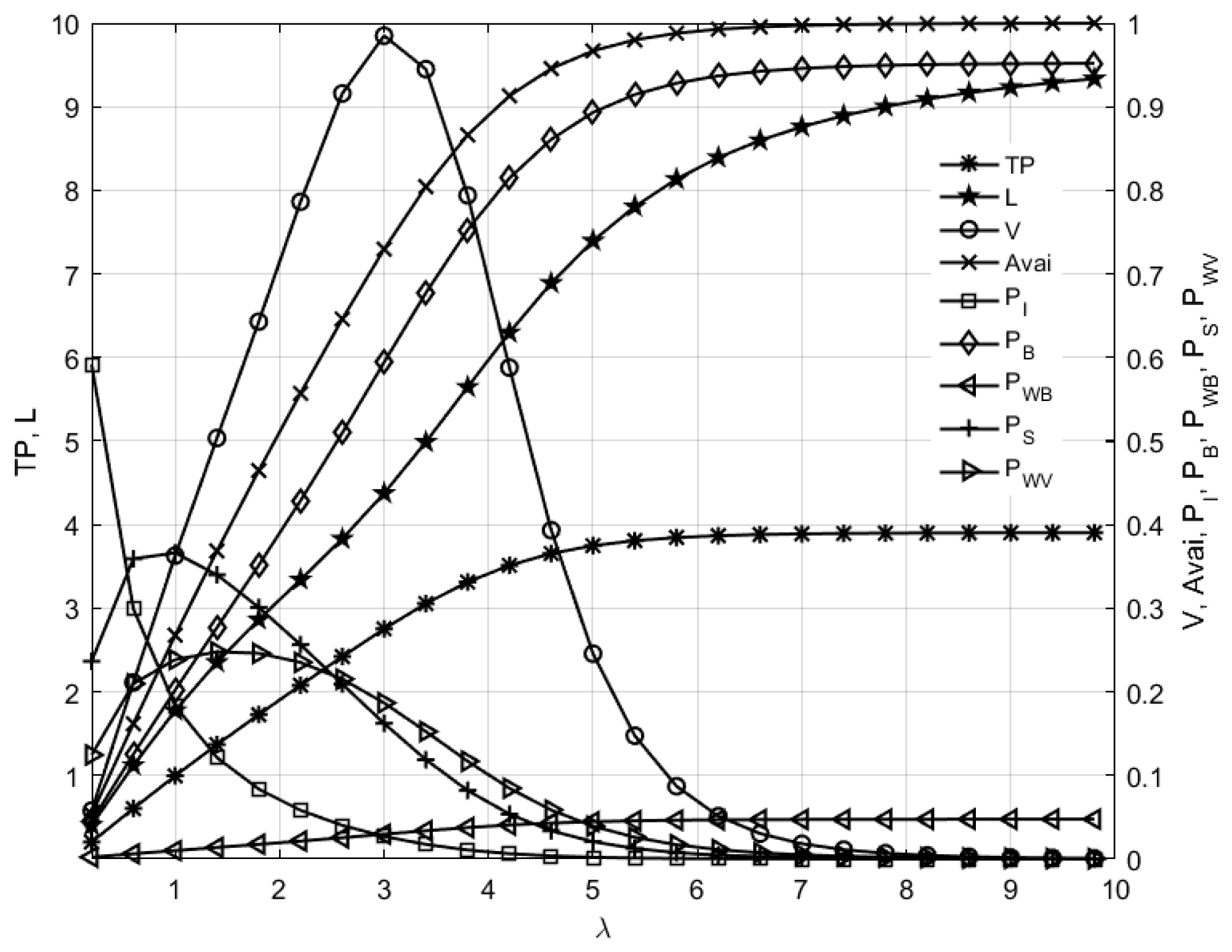
Figure 3, Figure 4, Figure 5, Figure 6, Figure 7 and Figure 8 illustrate the influence of $\lambda$, $\theta$, s, $\alpha$, $\beta$, ${\mu }_B$, ${\mu }_V$, and ${\mu }_F$ on system performance measures, with the parameter settings as $\lambda =2$, ${\mu }_B=4$, ${\mu }_V=3$, ${\mu }_F=2$, $\theta =1$, $s=0.5$, $N=10$, and $\alpha =0.2$, $\beta =4$. Figure 3 reveals that the variations in system performance measures are rather significant as $\lambda$ changes. Specifically, $TP$, L, $Avai$, $P_B$, and $P_{WB}$ increase with $\lambda$, while $P_I$ decreases with $\lambda$. Moreover, V, $P_S$, and $P_{WV}$ first increase and then decrease with $\lambda$. The primary reason for the trends observed in $TP$, L, $Avai$, $P_B$, $P_{WB}$, and $P_I$ is that as the parameter $\lambda$ increases, more customers enter the system per unit time. Consequently, the total probability that the system is in an idle period will decline. When $\lambda$ is relatively small, due to the service rate of the system, it may frequently enter the idle or vacation state, which leads to an increase in $P_S$ and $P_{WV}$. However, as $\lambda$ further increases, the service rate can no longer meet the incoming customer demand, causing $P_S$ and $P_{WV}$ to decrease. Furthermore, with the increase in $\lambda$, the uncertainty and volatility faced by the system also rise accordingly, increasing V. As $\lambda$ continues to increase further, the entire system will gradually reach a relatively saturated state, and V will then decrease.

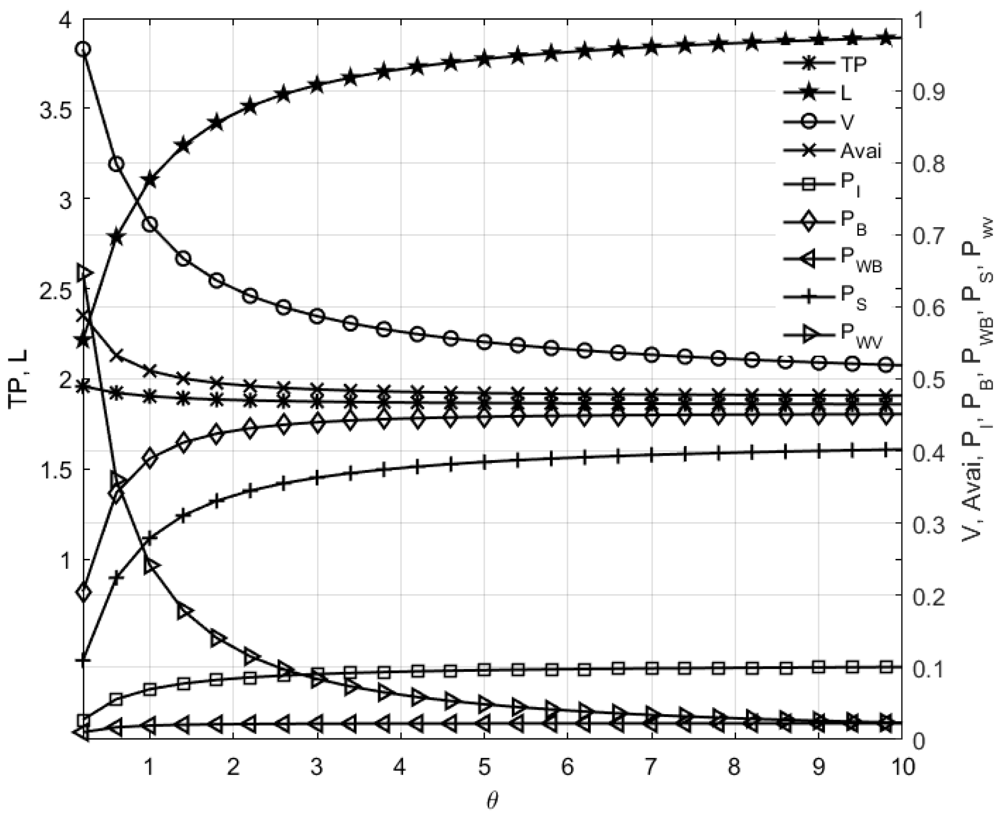
Figure 4 illustrates that V, $TP$, and $Avai$ as well as $P_{WV}$ decrease, while L, $P_I$, $P_S$, $P_B$, and $P_{WB}$ increase as $\theta$ increases. Among those, the impact of $\theta$ on $P_{WV}$ is the most pronounced, whereas its effect on $P_{WB}$ is the least significant. It should be emphasized that, based on no assumption in Section 2, we can derive that the length of the average vacation time is $1/$$\theta$. The average vacation time decreases as $\theta$ increases, and it will become extremely short when $\theta$ is relatively large. The reduction in the average vacation time can mitigate certain uncertain factors resulting from the server’s frequent vacations, thus causing V and $P_{WV}$ to decline. Moreover, given the same $\lambda$ and service rate, especially during the working vacation period, L, $P_I$, $P_S$, $P_B$ and $P_{WB}$ will generally increase, while $TP$ or $Avai$ will tend to decrease. However, since the server can still work during the working vacation, the impact of $\theta$ on $TP$ and $Avai$ is not particularly significant.

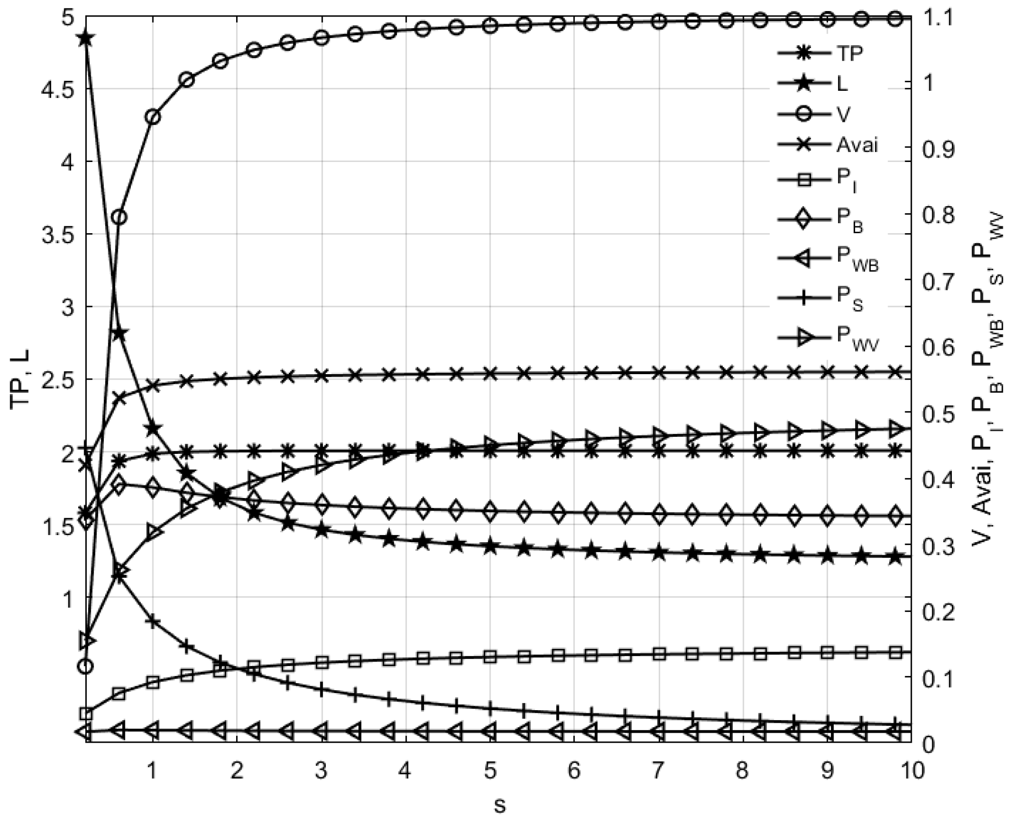
Figure 5 illustrates that as s increases, $TP$, V, $Avai$, $P_I$, and $P_{WV}$ increase, while L and $P_S$ decrease. By comparison, $P_B$ and $P_{WB}$ initially increase with the growth of s and tend to decrease gradually. Similar to the situation with $\theta$, the average setup time, which is 1/s, decreases as s increases, and it will become extremely short when s is relatively large. With the reduction in the average setup time, the server can obtain more effective service time and can largely reduce the uncertainties arising from fluctuations in setup time. This gives rise to the observed trends in $TP$, V, $Avai$, $P_I$, $P_{WV}$, L, and $P_S$. It also leads to an increase in $P_B$ and $P_{WB}$ when s is relatively small at the outset, but they will decrease slightly as the system adapts to the changes. Considering Figure 4 and Figure 5 comprehensively, when $\theta$ or s is small, that is to say, 1/$\theta$ or 1/s is large, the changing trends of various performance measures are relatively conspicuous. And as $\theta$ or s increases, the changing trends become more gradual. We can observe that if the average vacation time and average setup time are short, the impact on the performance measures will be much less significant.

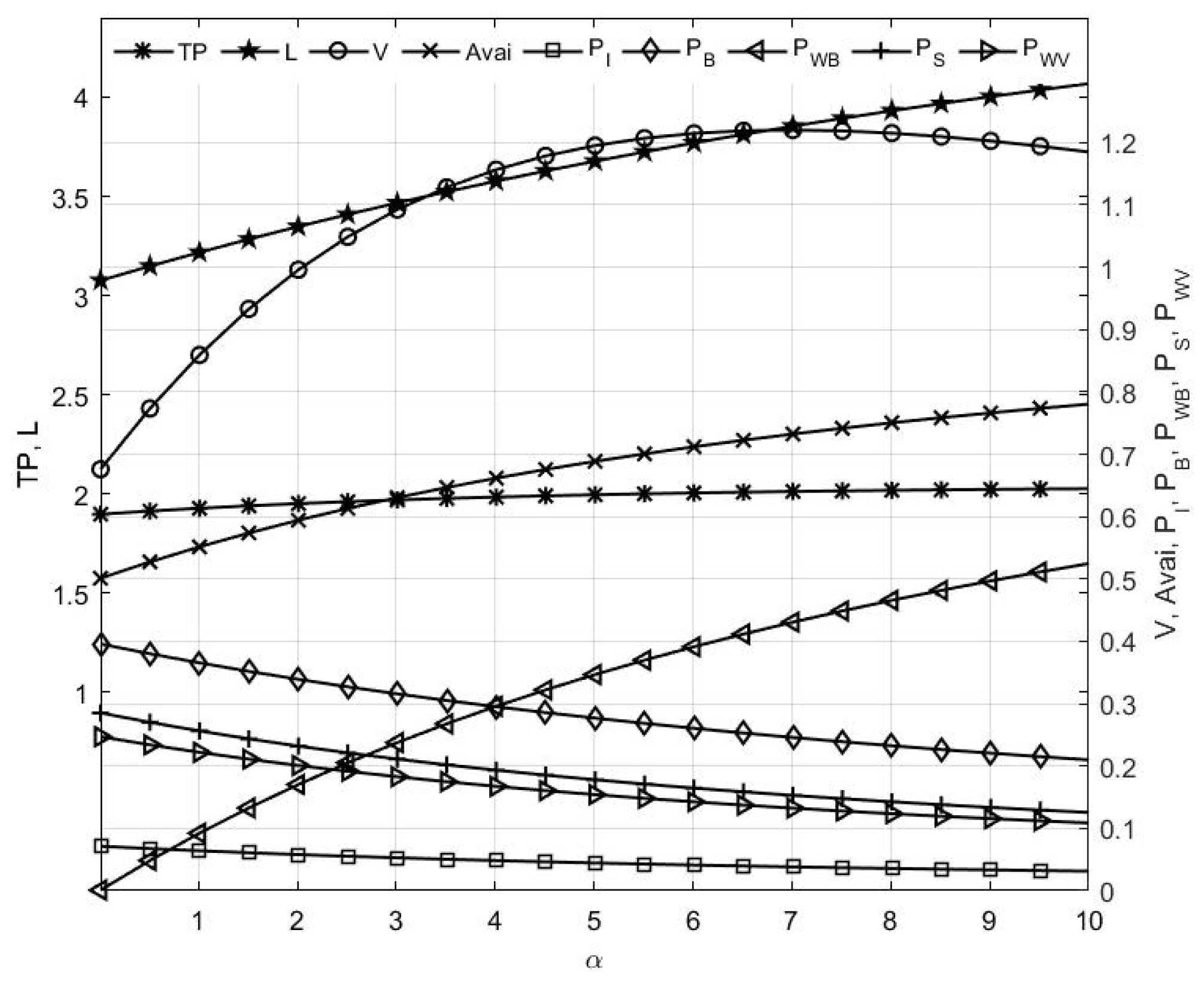
Figure 6 and Figure 7 illustrate the impact of the server breakdown rate $\alpha$ and the repair time parameter $\beta$ on system performance measures. Figure 6 reveals that $TP$, $Avai$, L, V, and $P_{WB}$ all increase as $\alpha$ increases, while $P_I$, $P_S$, $P_B$, and $P_{WV}$ decrease. With $\alpha$ increases, the mean time between failures, which is 1/$\alpha$, will decrease. However, since the server can still work during the breakdown period, $TP$, $Avai$, and $P_{WB}$ will increase with the growth of $\alpha$. Meanwhile, breakdowns introduce instability into the system, and the service rate during the breakdown period is slower than in the busy period. This leads to an increase in L and V. Moreover, with the increase in the state of working breakdown and the rise in the probability of working breakdown $P_{WB}$, the probabilities of other states, such as $P_I$, $P_S$, $P_B$, and $P_{WV}$, will decline.

Figure 7 illustrates that $P_I$, $P_S$, $P_B$, and $P_{WV}$ increase as $\beta$ increases, while $TP$, $Avai$, L, V, and $P_{WB}$ all decrease. As $\beta$ increases, the average repair time, which is 1/$\beta$, will decrease. The changing trends of the performance measures are precisely the opposite of those of $\alpha$. Since the server continues to work at the service rate ${\mu }_F$ after a breakdown occurs, the influence on system performance measures tends to level off when $\beta$ reaches a certain value. Compared to $\alpha$, $\beta$ has a smaller impact on the system performance measures.

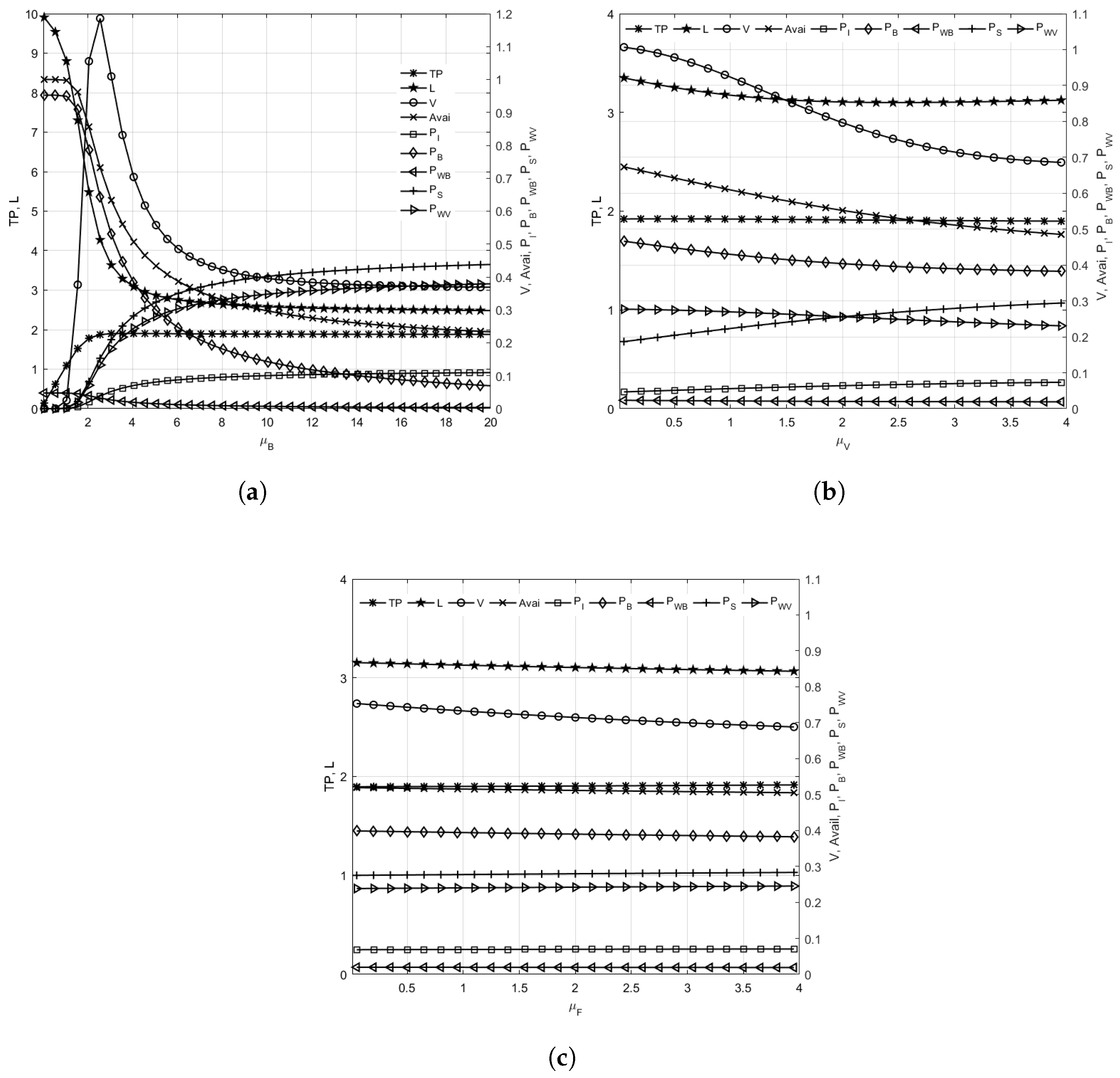
Figure 8 demonstrates that variations in ${\mu }_B$ exert the most pronounced influence on system performance measures, whereas changes in ${\mu }_V$ have the least effect. Specifically, Figure 8a–c illustrate that $Avai$, $P_B$, and $P_{WB}$ decrease as ${\mu }_B$, ${\mu }_V$, and ${\mu }_F$ increase. Conversely, $TP$, $P_I$, and $P_S$ increase with rising ${\mu }_B$, ${\mu }_V$, and ${\mu }_F$. V decreases with increasing ${\mu }_V$ and ${\mu }_F$ but increases with increasing ${\mu }_B$. L decreases with increasing ${\mu }_B$ and ${\mu }_F$ but increases with increasing ${\mu }_V$. $P_{WV}$ increases with increasing ${\mu }_B$ and ${\mu }_F$ but decreases with increasing ${\mu }_V$. Notably, the most effective approach to boosting system throughput rate $TP$ and reducing output variance V is to enhance the service rate during working vacation ${\mu }_V$ and the service rate during working breakdown ${\mu }_F$. Although improving the service rate during the regular busy period ${\mu }_B$ can improve the system throughput rate $TP$, it concurrently elevates output variance V. The result further confirms the necessity to study the strategies of working vacations and working breakdowns in queueing system.

6.2. Sensitivity Analysis of the Cost Optimization Function

This section delves into the impact of decision variables and cost coefficients on the cost optimization function $F({\mu }_B,{\mu }_V,{\mu }_F)$. In this study, the parameters are set as $N=10$, $\lambda =2$, ${\mu }_B=4$, ${\mu }_V=2$, ${\mu }_F=3$, $\theta =1$, $s=2$, $\alpha =0.5$, $\beta =2$, $c_L=5$, $c_I=2$, $c_S=3$, $c_B=350$, $c_{WV}=20$, $c_{WB}=80$, $c_{{\mu }_B}=10$, $c_{{\mu }_V}=6$, $c_{{\mu }_F}=6$, Subsequently, the cost optimization function is analyzed by varying the decision variables.

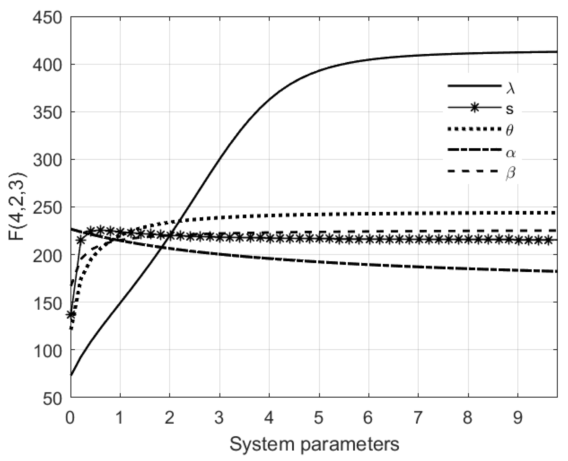
Figure 9, Figure 10 and Figure 11 illustrate the influence of buffer capacity N, ${\mu }_B$, ${\mu }_V$, ${\mu }_F$, $\lambda$, s, $\theta$, $\alpha$, and $\beta$ on the cost optimization function F, respectively. As shown in Figure 9, F increases as N increases, and it has a more significant impact when N is small. Once N reaches a certain value, the change curve of F levels off, and the impact of N on F becomes negligible. Figure 10 indicates that F increases with $\lambda$, $\theta$, and $\beta$, while F decreases while $\alpha$ increases. Meanwhile, when s is relatively small, that is to say when the mean setup time 1/s is large, F increases as s increases. However, it soon tends to decrease as s increases. F is greatly influenced by $\lambda$, s, and $\theta$. This means that higher customer arrival rates, longer setup time, and vacation time will all result in higher costs. As a whole, the change trend of F tends to level off when $\lambda$, s, $\theta$, $\alpha$, and $\beta$ increase to a certain value.

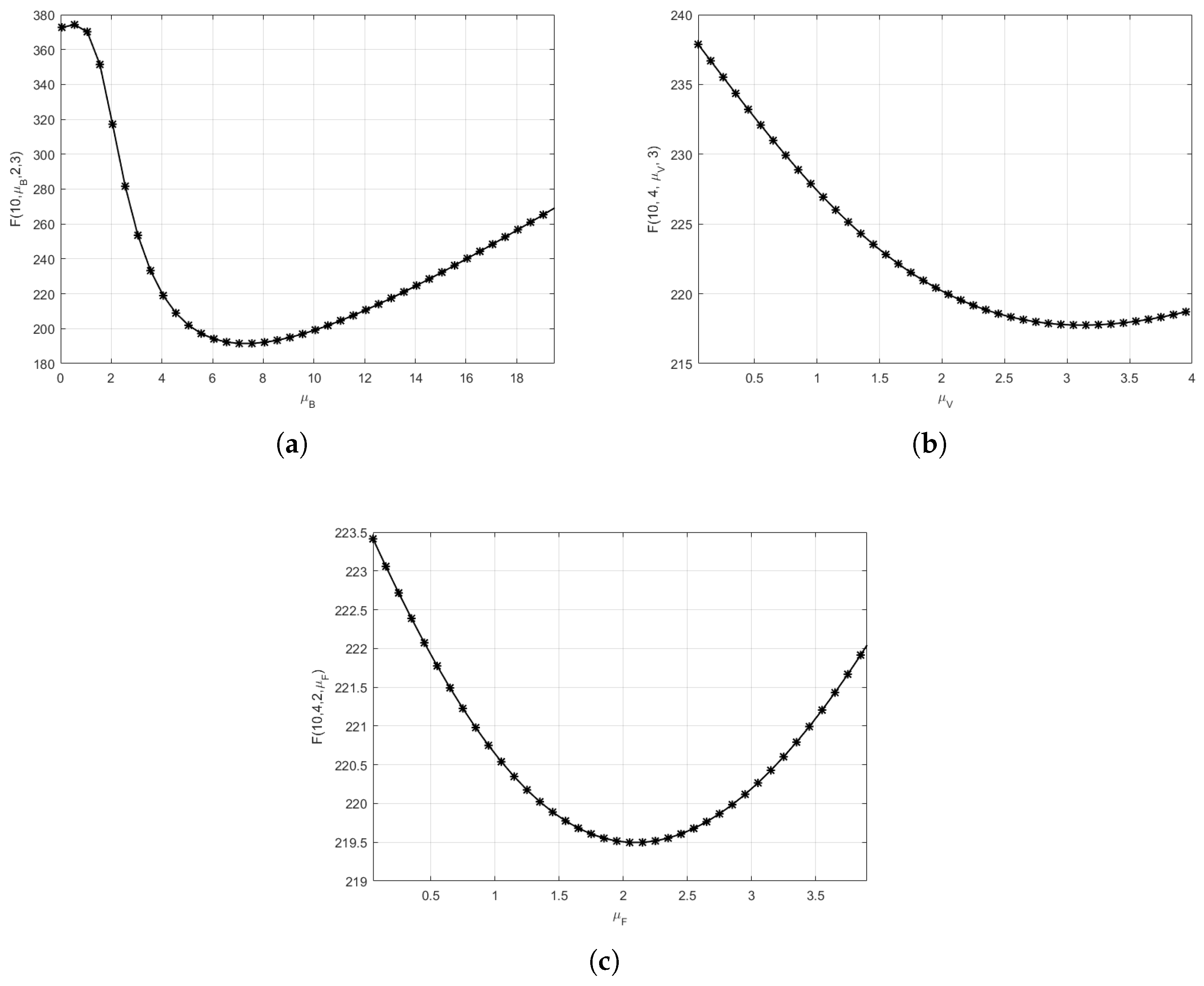
Correspondingly, Figure 11a–c demonstrate that F first decreases and then increases as ${\mu }_B$, ${\mu }_V$, and ${\mu }_F$ increase. In other words, F has an inflection point in the change process of ${\mu }_B$, ${\mu }_V$, and ${\mu }_F$, indicating that there are optimal solutions for the service rates.

Figure 12 depicts the influence of the cost coefficients $c_L$, $c_I$, $c_S$, $c_B$, $c_{WV}$, $c_{WB}$, $c_{{\mu }_B}$, $c_{{\mu }_V}$, and $c_{{\mu }_F}$ on the cost optimization function. As observed from the figure, the cost optimization function shows a generally linear increasing trend with the increase in each cost coefficient. Specifically, $c_L$, $c_{{\mu }_B}$, $c_{{\mu }_V}$, and $c_{{\mu }_F}$ have a more significant impact on the cost optimization function F(${\mu }_B$, ${\mu }_V$, ${\mu }_F$) under the parameter settings ${\mu }_B=4$, ${\mu }_V=2$, and ${\mu }_F=3$. This is because the values of L, ${\mu }_B$, ${\mu }_V$, and ${\mu }_F$ are considerably higher than those of $P_I$, $P_S$, $P_B$, and $P_{WB}$.

6.3. Optimization Analysis of Cost Optimization Function

To evaluate the suitability and efficiency of SSA for solving the nonlinear cost optimization in the M/M/1/N WV and WB queueing system, we address the problems listed in

Table 2. The search results of PSO, CS and SSA.

$(\mathit{\lambda },\mathit{\theta },\mathit{s},\mathit{\alpha },\mathit{\beta })$	PSO
	${\mathit{F}}^{*}$	${\mathit{\mu }}_{\mathit{B}}^{*}$	${\mathit{\mu }}_{\mathit{V}}^{*}$	${\mathit{\mu }}_{\mathit{F}}^{*}$	Mean	Max
(0.8, 0.2, 0.5, 2, 1)	71.0713	3.3910	1.3008	0.8448	1.10572	1.13416
(1.8, 0.5, 0.5, 2, 1)	96.6617	4.9554	1.2769	2.2022	1.26818	1.32063
(3, 0.5, 0.5, 2, 1)	114.2587	4.4687	2.4216	4.2888	1.18776	1.21466
(1.8, 0.1, 0.5, 2, 1)	91.1652	7.2137	2.8388	0.7249	1.30232	1.35421
(1.8, 0.5, 0.9, 2, 1)	95.3813	4.1226	1.3073	3.892	1.24235	1.26960
(1.8, 0.5, 0.9, 1, 1)	92.2048	3.3515	1.9473	2.5267	1.26412	1.28532
(1.8, 0.5, 0.9, 2, 0.5)	90.2650	2.8999	1.5020	2.8998	1.31724	1.38687
$(\mathit{\lambda },\mathit{\theta },\mathit{s},\mathit{\alpha },\mathit{\beta })$	CS
	${\mathit{F}}^{*}$	${\mathit{\mu }}_{\mathit{B}}^{*}$	${\mathit{\mu }}_{\mathit{V}}^{*}$	${\mathit{\mu }}_{\mathit{F}}^{*}$	Mean	Max
(0.8, 0.2, 0.5, 2, 1)	70.4989	2.3775	1.2884	1.2686	1.00000	1.00000
(1.8, 0.5, 0.5, 2, 1)	94.3731	2.9357	1.3609	2.9356	1.00000	1.00000
(3, 0.5, 0.5, 2, 1)	114.0640	4.2372	2.3050	4.2311	1.00000	1.00000
(1.8, 0.1, 0.5, 2, 1)	86.0849	2.9485	2.7834	2.7295	1.00000	1.00000
(1.8, 0.5, 0.9, 2, 1)	91.6702	3.0552	1.8765	2.9599	1.00000	1.00000
(1.8, 0.5, 0.9, 1, 1)	89.9696	5.5602	2.2362	0.9533	1.00000	1.00000
(1.8, 0.5, 0.9, 2, 0.5)	90.2644	2.8927	1.4788	2.8926	1.00000	1.00000
$(\mathit{\lambda },\mathit{\theta },\mathit{s},\mathit{\alpha },\mathit{\beta })$	SSA
	${\mathit{F}}^{*}$	${\mathit{\mu }}_{\mathit{B}}^{*}$	${\mathit{\mu }}_{\mathit{V}}^{*}$	${\mathit{\mu }}_{\mathit{F}}^{*}$	Mean	Max
(0.8, 0.2, 0.5, 2, 1)	70.4989	2.3759	1.2853	1.2718	1.00000	1.00000
(1.8, 0.5, 0.5, 2, 1)	94.3731	2.9345	1.3570	2.9344	1.00000	1.00000
(3, 0.5, 0.5, 2, 1)	114.064	4.2388	2.3039	4.2387	1.00000	1.00000
(1.8, 0.1, 0.5, 2, 1)	86.0849	2.9432	2.7778	2.7357	1.00000	1.00000
(1.8, 0.5, 0.9, 2, 1)	91.6702	3.0584	1.8768	2.9591	1.00000	1.00000
(1.8, 0.5, 0.9, 1, 1)	89.9696	5.5779	2.2318	0.9390	1.00000	1.00000
(1.8, 0.5, 0.9, 2, 0.5)	90.2644	2.8983	1.4757	2.8982	1.00000	1.00000

by conducting a comparative study against PSO and CS. All of the algorithms are run on PC equipped with 3.2 GHz, 16 GB, and a Intel single-core processor. For each test case, the special parameter settings are as follows: the buffer capacity is set to $N=15$, and the cost coefficients are defined as $c_L=5$, $c_I=2$, $c_S=50$, $c_B=75$, $c_{WV}=30$, $c_{WB}=45$, $c_{{\mu }_B}=4$, $c_{{\mu }_V}=2$, and $c_{{\mu }_F}=5$. Regarding the system parameters ${\mu }_B$, ${\mu }_V$, and ${\mu }_F$, their lower and upper bounds are ${\mu }_L$ = 0.5 and ${\mu }_U$ = 20, respectively. Table 1 presents the experimental results obtained from 200 independent experiments carried out using these three algorithms. To compare the effectiveness of the algorithms, the mean and maximum values of the ratio $F_{best}^{*}$/$F_{best}$ are adopted as evaluation criteria. Here, $F_{best}$ denotes the cost of the optimal solution obtained by the algorithms, while $F_{best}^{*}$ is the maximum value among the 200 experiments. Figure 13 depicts the convergence of the three algorithms for the third test case shown in Table 2.

Table 3. The CPU time for PSO, CS, and SSA.

$(\mathit{\lambda },\mathit{\theta },\mathit{s},\mathit{\alpha },\mathit{\beta })$	PSO	CS	SSA
(0.8, 0.2, 0.5, 2, 1)	373.6041	877.4292	592.4291
(1.8, 0.5, 0.5, 2, 1)	380.1668	1113.5692	613.4993
(3, 0.5, 0.5, 2, 1)	397.8724	3012.6651	587.5432
(1.8, 0.1, 0.5, 2, 1)	393.5976	877.0753	606.6444
(1.8, 0.5, 0.9, 2, 1)	395.3651	834.2787	656.0716
(1.8, 0.5, 0.9, 1, 1)	406.7137	945.1267	660.4522
(1.8, 0.5, 0.9, 2, 0.5)	402.1338	1553.0157	651.2009

presents the CPU time during the 200 experiments.

Based on the data presented in Figure 13 and Table 2 and Table 3, the following conclusions are derived:

• The average and maximum values of $F_{best}^{*}$/$F_{best}$ computed by the SSA are close to 1.00000, which implies that the SSA exhibits strong robustness and effective optimization capabilities throughout all test cases.
• The average and maximum values of $F_{best}^{*}$/$F_{best}$ calculated by the CS are also close to 1.00000; however, the SSA converges at a notably faster pace and is less likely to fall into local optima. The CPU calculation time for the SSA varies from 587.5432 s to 660.4522 s. In contrast, for the CS, it ranges from 834.2787 to 3012.6651 s. Not only is the CPU time of the SSA less variable, but it is also significantly shorter than that of the CS.
• The CPU calculation time for the PSO spans from 373.6041 to 406.3137 s, demonstrating a higher calculation speed compared to the SSA. However, the mean and maximum values of $F_{best}^{*}$/$F_{best}$ obtained by the PSO range from 1.10572 to 1.31742 and from 1.13416 to 1.38687, respectively, which indicates poor robustness. Moreover, the convergence speed of the PSO is significantly slower than that of the SSA.

As summarized above, considering comprehensively from convergence speed, solution accuracy, robustness, and calculation speed, SSA has demonstrated its advantages in solving cost optimization problem proposed in the paper.

7. Conclusions

This paper conducts the performance analysis and cost optimization of an M/M/1/N queueing system with setup time, working vacation, and working breakdown strategies. In this kind of system, during the vacation and breakdown, the server is capable of continuing to serve customers at a lower speed. Working vacation and working breakdown strategies are highly effective in terms of energy conservation and enhancing operational efficiency, which have led to their widespread application in manufacturing, maintenance, and communication systems. By constructing a two-dimensional continuous-time Markov chain and applying a block matrix representation of the minimum generating element, a finite QBD process of the system is derived. Subsequently, the stationary probability vector is solved through the matrix geometric method, thereby enabling the determination of the system’s output variance, availability, throughput rate, and queue length, as well as various stationary probabilities. Furthermore, a cost optimization model is established to minimize total cost per unit time, taking the service rates at each stage of the server as parameters. The sensitivities of both the system performance and cost optimization functions are analyzed, and the SSA is employed to solve the optimization model. The QBD process, matrix geometric method, and SSA utilized in this paper provide a solid theoretical foundation for the study of complex queueing systems and their optimization. In future research, we plan to address diverse problems in real complex environments, aiming to expand the application scope of the queueing system. And we can also try to put forward algorithmic enhancements tailored specifically to these complex queuing model frameworks. For instance, it can be used to analyze and optimize patient flow by predicting and managing waiting times in a hospital setting, or to analyze and optimize the flow of energy in a smart grid, among other potential applications.

References

1. Guo, X.; Niu, Z.; Zhou, S.; Kumar, P. Delay-constrained energy-optimal base station sleeping control. IEEE J. Sel. Areas Commun. 2016, 34, 1073–1085. [Google Scholar] [CrossRef]
2. Xu, J.; Wu, X.; Huang, Q.; Sun, P. How Should the Server Sleep?—Age-Energy Tradeoff in Sleep-Wake Server Systems. IEEE Trans. Green Commun. Netw. 2023, 7, 1620–1634. [Google Scholar] [CrossRef]
3. Servi, L.D.; Finn, S.G. M/M/1 queues with working vacations (M/M/1/WV). Perform. Eval. 2002, 50, 41–52. [Google Scholar] [CrossRef]
4. Kalidass, K.; Kasturi, R. A queue with working breakdowns. Comput. Ind. Eng. 2012, 63, 779–783. [Google Scholar] [CrossRef]
5. Jain, M.; Sharma, G.C.; Sharma, R. Working vacation queue with service interruption and multi optional repair. Int. J. Inf. Manag. Sci. 2011, 22, 157–175. [Google Scholar]
6. Li, T.; Wang, Z.; Liu, Z. Geo/Geo/1 retrial queue with working vacations and vacation interruption. J. Appl. Math. Comput. 2012, 39, 131–143. [Google Scholar] [CrossRef]
7. Hu, C.; Zhu, Y. Equilibrium distributions of the queue length in Geo/Geo/1 queue system with negative customer, feedback and multiple working vacations. Syst. Eng.-Theory Pract. 2012, 2, 1494–1500. [Google Scholar] [CrossRef]
8. Liu, Z.; Song, Y. Geo/Geo/1 retrial queue with non-persistent customers and working vacations. J. Appl. Math. Comput. 2013, 42, 103–115. [Google Scholar] [CrossRef]
9. Yu, M.; Alfa, A. Strategic queueing behavior for individual and social optimization in managing discrete time working vacation queue with Bernoulli interruption schedule. Comput. Oper. Res. 2016, 73, 43–55. [Google Scholar] [CrossRef]
10. Yang, B.; Hou, Z.; Wu, J. Analysis of the equilibrium strategies in the Geo/Geo/1 queue with multiple working vacations. Qual. Technol. Quant. Manag. 2017, 15, 663–685. [Google Scholar] [CrossRef]
11. Barbhuiya, F.; Gupta, U. A Discrete-Time GIX/Geo/1 Queue with Multiple Working Vacations Under Late and Early Arrival System. Methodol. Comput. Appl. Probab. 2020, 22, 599–624. [Google Scholar] [CrossRef]
12. Wu, S.; Lan, S. Analysis of repairable discrete-time queueing systems with negative customers, disasters, balking customers and interruptible working vacations under Bernoulli schedule. Math. Comput. Simul. 2025, 232, 102–122. [Google Scholar] [CrossRef]
13. Artalejo, J.; Gómez-Corral, A. Retrial Queueing Systems: A Computational Approach; Springer: Berlin/Heidelberg, Germany, 2008. [Google Scholar]
14. Atencia-Mckillop, I.; Sánchez-Merino, S.; Fortes-Ruiz, I.; Galán-García, J.L. Discrete-Time Retrial Queuing Systems with Last Come-First-Served (LCFS) and First-Come-First-Served (FCFS) Disciplines: Negative Customer Impact and Stochastic Analysis. Mathematics 2025, 13, 107. [Google Scholar] [CrossRef]
15. Rajadurai, P.; Saravanarajan, M.C.; Chandrasekaran, V.M. A study on M/G/1 feedback retrial queue with subject to server breakdown and repair under multiple working vacation policy. Alex. Eng. J. 2018, 57, 947–962. [Google Scholar] [CrossRef]
16. Sun, W.; Li, S.; Wang, Y.; Tian, N. Comparisons of exhaustive and non-exhaustive M/M/l/N queues with working vacation and threshold policy. J. Syst. Sci. Syst. Eng. 2019, 28, 154–167. [Google Scholar] [CrossRef]
17. Li, S.; Yang, X.; Peng, D.; Chen, J. Analysis of M/M/1/N working vacation queueing system with setup times and repairable service station. Control Decis. 2020, 35, 319–328. [Google Scholar]
18. Jain, M.; Dhibar, S.; Sanga, S.S. Markovian working vacation queue with imperfect service, balking and retrial. J. Ambient Intell. Humaniz. Comput. 2022, 13, 1907–1923. [Google Scholar] [CrossRef]
19. Majid, S. Analysis of customer’s impatience in queues with Bernoulli schedule server working vacations and vacation interruption. Afr. Mat. 2022, 33, 1–13. [Google Scholar] [CrossRef]
20. Ammar, S.; Alharbi, Y.; Zhao, Y. Analysis of Vacation Fluid M/M/1 Queue in Multi-Phase Random Environment. Mathematics 2023, 11, 4444. [Google Scholar] [CrossRef]
21. Sindhu, S.; Krishnamoorthy, A.; Kozyrev, D. On Queues with Working Vacation and Interdependence in Arrival and Service Processes. Mathematics 2023, 11, 2280. [Google Scholar] [CrossRef]
22. Lai, C.; Kasim, E.; Muhammadhaji, A. Dynamic Analysis of a Standby System with Retrial Strategies and Multiple Working Vacations. Mathematics 2024, 12, 3999. [Google Scholar] [CrossRef]
23. Vijaya Laxmi, P.; Girija Bhavani, E.; George, A.A. Retention of impatient customers in a multi-server Markovian queueing system with optional service and working vacations. Commun. Stat.-Theory Methods 2023, 52, 5195–5212. [Google Scholar] [CrossRef]
24. Liu, T.H.; Chiou, K.C.; Chen, C.M.; Chang, F.M. Multiserver Retrial Queue with Two-Way Communication and Synchronous Working Vacation. Mathematics 2024, 12, 1163. [Google Scholar] [CrossRef]
25. Sundarapandiyan, S.; Nandhini, S. Sensitivity analysis of a non-Markovian feedback retrial queue, reneging, delayed repair with working vacation subject to server breakdown. Int. J. Math. Eng. Manag. Sci. 2024, 9, 21025–21052. [Google Scholar] [CrossRef]
26. Lv, S.; Yin, S.; Zan, Y. The queueing inventory system with working vacations and breakdowns. IAENG Int. J. Appl. Math. 2024, 54, 2198–2208. [Google Scholar]
27. Fiems, D. Queues with Working Vacations: A Survey. Mathematics 2025, 13, 1894. [Google Scholar] [CrossRef]
28. Ma, Z.; Cui, G.; Wang, P. M/M/1 vacation queueing system with working breakdowns and variable arrival rate. J. Comput. Inf. Syst. 2015, 11, 1–8. [Google Scholar]
29. Chen, J.; Yen, T.; Wang, K. Cost optimization of a single-server queue with working breakdowns under the N policy. J. Test. Eval. 2016, 44, 2059–2067. [Google Scholar] [CrossRef]
30. Jiang, T.; Xin, B. Computational analysis of the queue with working breakdowns and delaying repair under a Bernoulli-schedule-controlled policy. Commun. Stat.-Theory Methods 2019, 48, 926–941. [Google Scholar] [CrossRef]
31. Yang, X.; Li, Z.; Li, S.; Wu, F. Performance analysis of M/M/1/N queue with setup time and working breakdown. Control Theory Appl. 2019, 36, 561–569. [Google Scholar]
32. Li, J.; Li, T. An MX/G/1 G-queue with single vacation, setup time and working breakdown. Eng. Lett. 2020, 28, 1100–1107. [Google Scholar]
33. Zhang, M.; Gao, S. The disasters queue with working breakdowns and impatient customers. RAIRO-Oper. Res. 2020, 54, 815–825. [Google Scholar] [CrossRef]
34. Yen, T.C.; Wang, K.; Chen, J. Optimization analysis of the N policy M/G/1 queue with working breakdowns. Symmetry 2020, 12, 583. [Google Scholar] [CrossRef]
35. Yang, D.; Chen, Y.; Wu, C. Modelling and optimisation of a two-server queue with multiple vacations and working breakdownsn. Int. J. Prod. Res. 2020, 58, 3036–3048. [Google Scholar] [CrossRef]
36. Yang, D.; Wu, C. Evaluation of the availability and reliability of a standby repairable system incorporating imperfect switchovers and working breakdowns. Reliab. Eng. Syst. Saf. 2021, 207, 1–16. [Google Scholar] [CrossRef]
37. Li, T.; Zhang, L. Discrete-time Geo/Geo/1 queue with negative customers and working breakdowns. IAENG Int. J. Appl. Math. 2017, 47, 442–448. [Google Scholar]
38. Lan, S.; Tang, Y. Performance analysis of a discrete-time queue with working breakdowns and searching for the optimum service rate in working breakdown period. J. Syst. Sci. Inf. 2017, 5, 176–192. [Google Scholar] [CrossRef]
39. Lv, S.; Li, F.; Li, J. The M/M/c retrial queueing system with impatient customers and server working breakdown. IAENG Int. J. Appl. Math. 2024, 54, 1499–1506. [Google Scholar]
40. Wu, C.; Yang, D.; He, T. Matrix-augmentation approach for machine repair problem with generally distributed repair times during working breakdown periods. Math. Comput. Simul. 2024, 225, 1019–1038. [Google Scholar] [CrossRef]
41. Jain, M.; Sharma, R.; Meena, R.K. Performance modeling of fault-tolerant machining system with working vacation and working breakdown. Arab. J. Sci. Eng. 2018, 44, 2825–2836. [Google Scholar] [CrossRef]
42. Rajadurai, P. Sensitivity analysis of an M/G/1 retrial queueing system with disaster under working vacations and working breakdowns. RAIRO-Oper. Res. 2018, 35, 913–930. [Google Scholar] [CrossRef]
43. Yang, D.; Chung, C.; Wu, C. Sojourn times in a Markovian queue with working breakdowns and delayed working vacations. Comput. Ind. Eng. 2021, 156, 1–13. [Google Scholar] [CrossRef]
44. Yang, X.; Li, Z.; Wang, H.; Wu, F. Performance analysis of M/M/1/N queueing system with working vacation and working breakdown. Control Theory Appl. 2021, 38, 2031–2044. [Google Scholar]
45. Jain, A.; Raychaudhuri, C. Cost optimization using Genetic Algorithm in customers intolerance Markovian model with working vacation and multiple working breakdowns. Int. J. Math. Eng. Manag. Sci. 2022, 7, 656–669. [Google Scholar] [CrossRef]
46. Manoharan, P.; Subathra, S. Non Markovian retrial queue, balking, disaster under working breakdown and working vacation. J. Comput. Anal. Appl. 2023, 31, 244–255. [Google Scholar]
47. Thakur, S.; Jain, A.; Ahuja, A. Analysis of MAP/PH/1 model with working vacation, working breakdown and two-phase repair. Arab. J. Sci. Eng. 2024, 49, 7431–7451. [Google Scholar] [CrossRef]
48. Nisha; Upadhyaya, S.; Shekhar, C. Maximum entropy solution for MX/G/1 priority reiterate G-queue under working breakdown and working vacation. Int. J. Math. Eng. Manag. Sci. 2024, 9, 163–187. [Google Scholar] [CrossRef]
49. Liu, T.H.; Hsu, H.Y.; Chang, F.M. Multi-server two-way communication retrial queue subject to disaster and synchronous working vacation. Algorithms 2025, 18, 24. [Google Scholar] [CrossRef]
50. Neuts, M. Matrix-Geometric Solution in Stochastic Models; The Johns Hopkins University Press: Baltimore, MD, USA, 1981. [Google Scholar]
51. Tian, N.; Yue, D. Quasi Birth and Death Process and Matrix Geometric Solution; Science Press: Beijing, China, 2002. [Google Scholar]
52. Elhafs, E.H.; Molle, M. On the solution to QBD processes with finite state space. Stoch. Anal. Appl. 2007, 25, 763–779. [Google Scholar] [CrossRef]
53. Kemeny, J.G.; Snell, J.L. Finite MARKOV Chains; Springer: New York, NY, USA, 1976. [Google Scholar]
54. Kemeny, J.G. Generalization of a fundamental matrix. Linear Algebra Its Appl. 1981, 38, 193–206. [Google Scholar] [CrossRef]
55. Xue, J.; Shen, B. A novel swarm intelligence optimization approach: Sparrow search algorithm. Syst. Sci. Control Eng. 2020, 8, 22–34. [Google Scholar] [CrossRef]
56. Xue, J. Research and Application of a Novel Swarm Intelligence Optimization Technique: Sparrow Search Algorithm. Ph.D. Thesis, Donghua University, Shanghai, China, 2020. [Google Scholar]
57. Fu, H.; Liu, H. Improved sparrow search algorithm with multi-strategy integration and its application. Control Decis. 2022, 37, 87–96. [Google Scholar]
Figure 1. State transition diagram of the M/M/1/N WV and WB queueing system with setup time.
Mathematics 13 02980 g001
Figure 2. Influence of N on system performance measures.
Mathematics 13 02980 g002
Figure 3. Influence of λ on system performance measures.
Mathematics 13 02980 g003
Figure 4. Influence of θ on system performance measures.
Mathematics 13 02980 g004
Figure 5. Influence of s on system performance measures.
Mathematics 13 02980 g005
Figure 6. Influence of α on system performance measures.
Mathematics 13 02980 g006
Figure 7. Influence of β on system performance measures.
Mathematics 13 02980 g007
Figure 8. Influence of parameters of the service rates in different states on system performance measures. (a) μ B . (b) μ V . (c) μ F .
Mathematics 13 02980 g008
Figure 9. Influence of buffer capacity N on F(4,2,3).
Mathematics 13 02980 g009
Figure 10. Influence of λ , s, θ , α , β on F(4,2,3).
Mathematics 13 02980 g010
Figure 11. Influence of parameters of the service rates in different states on F ( μ B , μ V , μ F ) . (a) μ B . (b) μ V . (c) μ F .
Mathematics 13 02980 g011
Figure 12. Influence of cost coefficients on F(4,2,3).
Mathematics 13 02980 g012
Figure 13. Optimizing convergence rates of SSA, CS, and PSO.
Mathematics 13 02980 g013