A Reinforcement Learning-Assisted Fractional-Order Differential Evolution for Solving Wind Farm Layout Optimization Problems

Abstract

The Wind Farm Layout Optimization Problem (WFLOP) aims to improve wind energy utilization and reduce wake-induced power losses through optimal placement of wind turbines. Genetic Algorithms (GAs) and Particle Swarm Optimization (PSO) have been widely adopted due to their suitability for discrete optimization tasks, yet they suffer from limited global exploration and insufficient convergence depth. Differential evolution (DE), while effective in continuous optimization, lacks adaptability in discrete and nonlinear scenarios such as WFLOP. To address this, the fractional-order differential evolution (FODE) algorithm introduces a memory-based difference mechanism that significantly enhances search diversity and robustness. Building upon FODE, this paper proposes FQFODE, which incorporates reinforcement learning to enable adaptive adjustment of the evolutionary process. Specifically, a Q-learning mechanism is employed to dynamically guide key search behaviors, allowing the algorithm to flexibly balance exploration and exploitation based on problem complexity. Experiments conducted across WFLOP benchmarks involving three turbine quantities and five wind condition settings show that FQFODE outperforms current mainstream GA-, PSO-, and DE-based optimizers in both solution quality and stability. These results demonstrate that embedding reinforcement learning strategies into differential frameworks is an effective approach for solving complex combinatorial optimization problems in renewable energy systems.

1. Introduction

In the context of a profound global energy transition and the rise of green, low-carbon economies, renewable energy is expanding rapidly and playing an increasingly pivotal role in restructuring energy systems. As fossil fuel resources diminish and carbon emissions exacerbate climate change, the deployment of renewable technologies has become a strategic priority to ensure energy security and address environmental challenges [1,2]. Among various renewable sources, wind energy stands out as a clean, sustainable, and economically viable option. Due to its low carbon footprint and vast potential, wind power has emerged as a key component of national energy infrastructures [3,4]. Supported by technological advances and favorable policies, the global share of wind-generated electricity continues to rise, reinforcing its role in sustainable energy systems. Despite these achievements, large-scale wind energy deployment faces technical and economic challenges, including high initial investment, power output variability, and energy losses caused by aerodynamic wake effects [5,6,7]. Wake interactions notably reduce wind speed for downstream turbines, lowering their efficiency and overall farm output. To address these issues, the Wind Farm Layout Optimization Problem (WFLOP) has received growing attention. Its goal is to optimize turbine placement to reduce wake interference and maximize energy yield. Solving the WFLOP requires precise modeling of aerodynamic interactions, along with consideration of terrain, land use, costs, and environmental impact [8,9]. Given its multi-objective, high-dimensional, and nonlinear nature, the WFLOP serves as a challenging benchmark for metaheuristic optimization and an active research area across computational fluid dynamics, algorithm design, and energy systems. Progress in WFLOP modeling and solution methods is thus vital for improving wind energy performance and contributing to global climate and energy goals.

The WFLOP presents intrinsic difficulties due to its highly nonlinear and discrete solution space, which significantly increases the problem’s computational complexity and limits the effectiveness of traditional optimization strategies. A major challenge lies in the complex aerodynamic wake interactions among turbines: when upstream turbines extract wind energy, they generate turbulent wake zones that reduce wind speed for downstream turbines, leading to a nonlinear and spatially variable power generation environment [10]. Additionally, turbine placements are typically restricted to a finite set of candidate locations to comply with land use, topography, and safety regulations, rendering the WFLOP a combinatorial optimization problem with high-dimensional discrete decision variables [11]. Due to these combined effects, the WFLOP often exhibits non-convex landscapes with many local optima and is widely considered NP-Hard, making it difficult for classical mathematical methods to find global optima in polynomial time. To address these challenges, metaheuristic algorithms have emerged as promising solutions, owing to their global search capabilities and flexibility in handling non-differentiable, high-dimensional, and discrete problems [8,9]. Early studies employed Genetic Algorithms (GAs) and their adaptive versions (AGAs), which use population-based evolution and discrete encoding to optimize turbine layouts. These algorithms show good adaptability in combinatorial spaces but often suffer from premature convergence and parameter sensitivity [10,12]. Particle Swarm Optimization (PSO) and its evolutionary variants have also been widely applied due to their effective swarm intelligence mechanisms and fast convergence in continuous domains. However, PSO’s native design is more suited for continuous optimization, and its performance degrades in discrete layout scenarios due to limited global exploration and susceptibility to local optima [13,14]. While various improvements—such as adaptive parameter tuning and chaotic perturbations—have been proposed to mitigate these limitations, these algorithms still face difficulties in maintaining population diversity and stability in complex wind field environments. To overcome the inherent drawbacks of GAs and PSO-based methods in the WFLOP, differential evolution (DE) has gradually attracted attention due to its simple yet powerful mutation and selection operators. Some early applications of DE in wind farm layout optimization have demonstrated encouraging results, showing better balance between global and local search compared to other metaheuristics. However, adapting DE to discrete, large-scale, and combinatorial settings remains a key challenge and is the focus of ongoing research. Notably, DE has also shown superior performance in other renewable energy contexts, such as solar photovoltaic model parameter estimation [15], further validating its robustness in solving nonlinear, high-dimensional optimization problems.

Recent studies have demonstrated that the integration of intelligent control mechanisms—including adaptive strategy scheduling, surrogate model guidance, and reinforcement learning (RL)-based parameter tuning—can significantly enhance both the search efficiency and global performance of evolutionary optimization algorithms. RL is a type of machine learning that allows an agent to interact with its environment and iteratively learn optimal strategies based on reward signals. Unlike traditional supervised learning, RL does not rely on labeled datasets. Instead, it adapts through feedback from dynamic environments, making it particularly suitable for solving complex and time-varying optimization problems. In the field of evolutionary computation, RL has been widely adopted to enhance algorithm adaptability and search efficiency due to its ability to dynamically adjust strategies, parameters, and search behaviors. Specifically, RL mechanisms can utilize feedback during the optimization process—such as population quality, convergence rate, and diversity indicators—to adaptively tune key parameters including mutation rates, crossover probabilities, and selection pressures. Moreover, RL enables intelligent switching between multiple strategies in real time, thereby balancing global exploration and local exploitation and reducing the risk of premature convergence. For instance, Sun et al. [16] proposed an RL-assisted DE algorithm that integrates policy gradient reinforcement learning to dynamically adjust mutation factors and crossover rates. Their method allows the algorithm to autonomously adapt to different stages of the search process, resulting in significantly improved convergence speed and solution quality across various benchmark functions, with enhanced robustness and adaptability compared to traditional DE. Similarly, Guo et al. [17] employed deep reinforcement learning to perform dynamic algorithm selection within evolutionary algorithms. In their approach, the RL agent selects appropriate search strategies based on the current search state, enabling flexible adaptation to complex, high-dimensional, and nonlinear optimization problems. This effectively circumvents the limitations of manual parameter tuning and enhances both stability and performance. In the context of PSO, Tan et al. [18] proposed an adaptive Q-learning-based PSO algorithm specifically designed for multi-UAV path planning. Their method integrates a Q-learning (QL) mechanism to dynamically adjust the inertia weights and learning factors of particles based on environmental feedback. This adaptive strategy enables the algorithm to better balance global exploration and local exploitation, avoid premature convergence, and significantly improve convergence efficiency and solution quality in complex optimization tasks. In summary, reinforcement learning introduces a feedback-driven intelligent control mechanism into evolutionary algorithms, enabling them to adapt dynamically to changing environments and search conditions. This greatly enhances the automation of parameter tuning and overall optimization performance. In particular, for high-dimensional, nonlinear, and discrete combinatorial optimization problems, RL-assisted evolutionary algorithms have demonstrated faster convergence rates, stronger global search capabilities, and more stable performance. Consequently, RL-based evolutionary optimization has emerged as a prominent research focus and an important development direction in the field.

QL casts evolutionary search as a discrete Markov Decision Process (MDP) and iteratively approximates the optimal state–action value function via the Bellman optimality equation, guaranteeing convergence when $\sum {\alpha }_t=\infty$ and $\sum {\alpha }_t^2<\infty$ [19,20]. Compared with Policy-Gradient or SARSA controllers, QL’s off-policy nature enables exploration without perturbing the optimizer’s main trajectory, while its tabular implementation incurs only $O\left(\right|\mathcal{S}|\times |\mathcal{A}\left|\right)$ memory and computational cost—negligible relative to a single fitness evaluation. Recent studies, such as qlDE by Huynh et al. [21] and RLDE-AFL by Guo et al. [22], have demonstrated that QL can serve as an effective on-line parameter controller for differential evolution, achieving state-of-the-art performance on diverse black-box benchmarks. Motivated by the WFLOP’s discrete, highly non-stationary wake landscape, we adopt an offline multi-path pre-training + stage-wise on-line update scheme: (i) multiple Q-tables are pre-trained on historical populations and aggregated to yield a globally robust initial policy; (ii) the formal optimization run is partitioned into several stages, each maintaining an independent Q-table updated with a reward defined by the normalized remaining optimality gap. This design satisfies the classic exploration–exploitation annealing requirement—aggressive exploration early on and fine-grained exploitation later—while retaining the long-memory advantage of fractional-order differences. Consequently, it markedly enhances global escape capability and convergence stability, making it particularly well-suited to the complex combinatorial search characteristics of the WFLOP.

The adaptive differential evolution algorithm LSHADE, known for its innovations in parameter self-adaptation and linear population-size reduction, has achieved top performance across various continuous optimization benchmarks and is regarded as a milestone in DE research [23]. However, LSHADE and its variants are primarily designed for continuous decision spaces; when directly applied to the WFLOP characterized by discrete layouts, high combinatorial complexity, and rapidly increasing dimensionality, they often suffer from premature convergence due to insufficient search jumps and diminishing population diversity. To address this limitation, Tao et al. proposed the FODE (fractional-order difference-driven Evolution) algorithm [24], which incorporates fractional-order difference evolution into the LSHADE framework. In FODE, each individual is updated by fusing multiple historical generations with linearly decaying weights, which preserves local exploitation precision while significantly improving global escape ability and diversity regulation. Extensive WFLOP experiments have shown that FODE consistently outperforms GA, PSO, and several DE variants under various wind directions and layout scales. Although FODE enhances DE’s global search capability and historical memory through the introduction of fractional-order differences, its core control parameter a—which determines the fusion depth of historical generations—remains fixed throughout the optimization process. As a result, it fails to respond in real time to variations in wind field conditions, farm scale, and population dynamics. This fixed-depth memory design overlooks the temporal structure of the optimization landscape, which is particularly problematic in the WFLOP, a high-dimensional, strongly non-convex, and time-evolving problem. In early iterations, greater exploration is needed, whereas in later stages, the algorithm must gradually converge to fine local regions. Such annealing-like evolutionary behavior cannot be effectively captured within the static FODE mechanism. To overcome this shortcoming, we introduce a Q-learning-based intelligent regulation mechanism. As a model-free reinforcement learning method that supports offline learning and online adaptation, Q-learning treats the optimization as a state–action interaction system and continuously learns optimal control policies for different search stages through feedback from the environment—without interfering with the main evolutionary trajectory. Its structural advantages make it especially suitable for evolutionary processes where parameter adjustments rely heavily on environmental feedback and behavior must adapt to changing search states. It is particularly effective in tuning key parameters such as a, which critically influence search globality and memory depth. Based on these insights, we propose FQFODE, a hybrid evolutionary framework that integrates FODE with Q-learning. The core ideas are the following: (i) a Q-learning agent perceives the population state—including the current best power output, remaining optimality gap, and diversity metrics—and makes real-time decisions on the fractional difference coefficient and related search parameters, enabling adaptive switching between exploration and exploitation; (ii) given that the evolutionary process typically follows an annealing pattern of rapid expansion followed by fine convergence, we partition the full optimization horizon according to the remaining search space into multiple stages, each maintaining an independent Q-table. A normalized residual improvement reward scheme is adopted to eliminate learning interference caused by inter-stage difficulty disparities, achieving fine-grained control analogous to piecewise function approximation; (iii) to avoid single-path training bias and local overfitting, we propose a distributed collaborative multi-path pretraining strategy: multiple groups initialized with different random seeds and representative wind scenarios inherit and update their Q-tables in parallel. After several evolutionary rounds, the final Q-tables from each group are performance-weighted and aggregated to obtain a globally robust initial Q-table, which is used as prior knowledge during formal optimization and continues to be updated online to reflect the real-time search trajectory.This three-tier mechanism enables FQFODE to retain the long-memory global perspective of FODE while equipping it with environment-responsive agility. Consequently, the algorithm achieves both efficient convergence and significantly improved robustness and solution quality in extremely complex WFLOP scenarios.

(1)

This study proposes the FQFODE optimizer, which integrates a multi-path Q-learning pretraining framework with a stage-wise adaptive parameter control mechanism. It enables the effective application of the DE variant FODE to WFLOPs characterized by both discreteness and nonlinearity. By dynamically adjusting the fractional-order difference operator parameter a, FQFODE addresses the limitations of fixed parameter settings in conventional FODE when applied to highly heterogeneous WFLOP scenarios.

(2)

The experimental design in this paper draws from and extends recent advances by employing more realistic wind condition models and empirically accurate wind speed distributions. This ensures that the evaluation results and conclusions provide higher practical relevance and reliability.

(3)

Experimental evaluations and statistical analyses demonstrate the superior performance of the proposed FQFODE algorithm in solving the WFLOP. Notably, under wind farm layouts with 50 and 80 turbines, FQFODE significantly outperforms state-of-the-art WFLOP optimizers—including the latest variants of GA, PSO, and FODE—by achieving higher power generation efficiency while maintaining strong robustness across diverse wind conditions.

(4)

The proposed wind farm optimization model, the wind condition datasets used in the experiments, and the full implementation of the FQFODE algorithm will be released open-source at: https://github.com/SichenTao/ (accessed on 7 August 2025) This is intended to support further research and reproducibility in the WFLOP community.

The remainder of this paper is organized as follows: Section 2 presents the design rationale of the proposed FQFODE algorithm and its adaptability to the WFLOP problem. It provides detailed mathematical formulations and implementation procedures for the multi-path Q-learning pretraining and aggregation mechanism, as well as the stage-wise adjustment strategy for the fractional-order difference parameter. Section 3 reports the experimental performance of FQFODE under various complex wind field conditions and compares it with state-of-the-art optimization algorithms to demonstrate its advantages in terms of performance, robustness, and applicability. Finally, Section 4 summarizes the main contributions of this work and outlines future research directions for WFLOP optimization.

2. Methodology

This section provides a systematic description of the overall framework and key mechanisms of the proposed FQFODE algorithm. First, for wind field modeling, a tunable wind speed attenuation expression is constructed based on the Jensen wake model, providing a physically consistent and resolution-controllable foundation for WFLOP scenarios. This forms the basis for realistic wind condition simulations in the optimization process. Within the FODE framework, FQFODE introduces a Q-learning-driven evolutionary optimization mechanism based on multi-path pretraining and collaborative Q-table fusion. Through distributed cooperative pretraining and inherited Q-table aggregation, FQFODE builds a control strategy for the critical parameter a, guided by dynamic feedback during the evolutionary process. This strategy enables intelligent and adaptive adjustment of the fractional-order difference control factor a, based on the current population’s power generation performance and diversity status. Furthermore, FQFODE divides the optimization process into four evolutionary stages, each associated with an independent Q-table. A stage-wise parameter adaptation strategy is employed, allowing the algorithm to exhibit enhanced adaptability and responsiveness across different phases of evolution. By integrating distributed experience aggregation with stage-specific strategy guidance, FQFODE significantly improves the search efficiency and robustness of the differential evolution algorithm in solving discrete–nonlinear coupled optimization problems. As a result, it offers a structurally clear and operationally effective solution framework for the WFLOP. Compared with existing Q-learning-enhanced DE variants such as qlDE and RLDE-AFL, which focus on tuning DE parameters (e.g., crossover rate or mutation factor), our method is the first to integrate Q-learning with a fractional-order difference evolutionary operator. This integration enables memory-depth regulation in the evolutionary trajectory, which is crucial for controlling the long-term influence of historical populations. Moreover, our three-tier architecture—consisting of distributed pretraining, federated knowledge aggregation, and stage-based adaptation—provides an environment-aware and phase-sensitive optimization strategy tailored specifically for the WFLOP.

2.1. Modeling

This study adopts the classical Jensen wake model [25,26] as the foundation for wind field simulation in WFLOP scenarios. Due to its simplicity, low computational cost, and solid accuracy in modeling wake-induced velocity deficits, the model has been widely adopted in WFLOP research [10,13]. It also allows integration of realistic wind variations without introducing significant computational overhead [27].

The wake effect is modeled based on momentum conservation, as illustrated in Figure 1. The downstream wind speed $V_2$ is derived from upstream conditions via the following equation:

$$\pi L_W^2{V}_1+\pi (L_X^2-L_W^2)V_0=\pi L_X^2{V}_2,$$

(1)

where $V_0$ is the free-stream wind speed, $L_W$ is the upstream rotor radius, $V_1$ is the wind speed just after the rotor, and $L_X$ is the expanded wake radius at distance X. The model computes $L_X$ and $V_1$ as follows:

$$L_X=L_W+X·tan\theta ,$$

(2)

$$V_1=(1-a)V_0,$$

(3)

The wake expansion angle $\theta$ depends on hub height h and terrain roughness $z_0$ and is calculated as follows:

$$\theta ={\displaystyle \frac{0.5}{ln\left(\frac{h}{z_0}\right)}}.$$

(4)

Typical values of $\theta$ range from 0.075 for onshore sites to 0.04 for smoother offshore terrains [26]. Incorporating this into the model yields the final expression for downstream wind speed:

$$V_2={\displaystyle \frac{L_W^2(1-a)V_0+\left({(L_W+X·tan\theta )}^2-L_W^2\right)V_0}{{\left(L_W+X·tan\theta \right)}^2}}.$$

(5)

To enhance realism, five wind scenarios are designed, each combining 2 to 6 wind directions with non-uniform magnitudes. Wind speeds follow a Weibull distribution with a mean of $13\mathrm{m}/\mathrm{s}$, which better captures the skewness of real wind profiles [28]. A high-resolution dataset of 100,000 samples is generated and used throughout the experiments.

All algorithms are evaluated under this unified modeling framework to ensure scientific rigor and comparability of results. Although not embedded directly into the algorithmic structure, the expressions derived in Section 2.1 serve as the objective function evaluator, being repeatedly called during the fitness evaluation phase of each optimization iteration.

2.2. Algorithmic Assumptions and Applicability

To make the premises of the proposed FODE/FQFODE framework explicit, we list four key modeling assumptions and discuss, for each, its rationale, expected validity range, and potential limitations.

1.

Wake–Flow Interaction Model: The classical Jensen wake model [25,26] is employed to capture momentum-deficit effects. Rationale—Its closed-form expression offers high computational efficiency and has been widely adopted in WFLOP benchmarks [10,13]. Validity— Flat terrain or offshore sites with turbulence intensity $\mathrm{TI}<0.15$ and turbine spacing $>3$–4 rotor diameters. Limitation—For complex topography or high-turbulence conditions, Jensen tends to under-predict wake recovery; CFD-calibrated or Ainslie models are recommended alternatives.

2.

Statistical Wind-Speed Representation: Long-term hub-height wind speed is modeled by a single-mode Weibull distribution with a mean of $13\mathrm{m}{\mathrm{s}}^{-1}$, from which ${10}^5$ samples are drawn (Figure 2). Rationale—Weibull distributions fit empirical annual wind records better than Gaussian or Rayleigh models [28]. Validity—Shape parameter $k\in [1.7,2.5]$ and scale parameter $c\in [6,10]\mathrm{m}{\mathrm{s}}^{-1}$. Limitation—Multi-modal or seasonally bimodal regimes may require mixture models.

3.

Wake Expansion Angle and Surface Roughness: The expansion coefficient $\theta$ follows Equation (4), with default values $\theta =0.075$ (onshore) and $\theta =0.04$ (offshore). Rationale—Values stem from Jensen’s calibration and subsequent field measurements [29]. Validity—Roughness length $z_0\in [0.02,0.3]\mathrm{m}$ and hub height $h\in [60,150]\mathrm{m}$. Limitation—Sites with $z_0>0.4\mathrm{m}$ (dense forests; mountainous terrain) necessitate roughness-dependent correction factors.

4.

Aerodynamic and Energy-Conversion Simplifications: Equations (1)–(5) invoke Betz’s law and neglect atmospheric stability, air-density variation, and turbulence feedback on power curves. Rationale—These simplifications keep objective evaluations $\mathcal{O}\left(1\right)$ per layout, enabling Q-learning inside FODE iterations. Validity—Mid-latitude regions where annual air-density fluctuations stay within $\pm 5\%$ of the IEC standard ($1.225\mathrm{kg}{\mathrm{m}}^{-3}$). Limitation—High-altitude or extreme climates may require density and power-curve corrections; such factors can be coupled via surrogate models without altering the core optimizer.

Under these assumptions, FODE and FQFODE maintain sub-quadratic runtime per generation and achieve competitive layout quality (Section 3). Outstanding challenges in extreme topography or multi-modal wind climates are noted for future work.

2.3. State-of-the-Art Differential Evolution

Differential evolution (DE) is a classical population-based optimization algorithm known for its simplicity and strong global search capability, particularly effective for NP-hard problems [30]. Among various DE variants, LSHADE stands out for its adaptive parameter control and linear population size reduction, achieving excellent results in numerous benchmark competitions [23,31].

FQFODE builds upon the LSHADE framework and enhances it through Q-learning-driven parameter adaptation. Within each generation, a population

$$P_x^{\left(k\right)}=\{x_1^{\left(k\right)},\dots ,x_{N{P}^{\left(k\right)}}^{\left(k\right)}\}$$

is evolved by differential operations. Individuals are initialized via uniform sampling within the search space:

$$x_{ij}^{\left(1\right)}=x_{lj}+(x_{hj}-x_{lj})·\mathrm{rand}(0,1],$$

(6)

Mutation is performed by combining elite and random solutions:

$${y^{\prime }}_{i,j}^{\left(k\right)}=x_{i,j}^{\left(k\right)}+s_i·\left(x_{pbes{t}_i,j}^{\left(k\right)}+x_{r_1,j}^{\left(k\right)}-x_{r_2,j}^{\left(k\right)}-x_{i,j}^{\left(k\right)}\right),$$

(7)

followed by binomial crossover:

$$y_{i,j}^{\left(k\right)}=\left\{\begin{array}{cc}{y^{\prime }}_{i,j}^{\left(k\right)}\hfill & \mathrm{if}j=j_{\mathrm{rand}}\vee \mathrm{rand}(0,1)<c_i,\hfill \\ x_{i,j}^{\left(k\right)}\hfill & \mathrm{otherwise},\hfill \end{array}\right.$$

(8)

and greedy selection:

$$x_{ij}^{(k+1)}=\left\{\begin{array}{cc}{y}_{ij}^{\left(k\right)},\hfill & \mathrm{if}f\left(y_i^{\left(k\right)}\right)\le f\left(x_i^{\left(k\right)}\right),\hfill \\ x_{ij}^{\left(k\right)},\hfill & \mathrm{otherwise},\hfill \end{array}\right.$$

(9)

To ensure adaptive control, the scaling factor $s_i$ and crossover rate $c_i$ are sampled from historical memory using Cauchy and normal distributions:

$$s_i^{\left(k\right)}=\mathrm{Cauchyrand}(L_{1m},0.1),c_i^{\left(k\right)}=\mathrm{Normrand}(L_{2m},0.1),$$

(10)

Reference values are updated based on the contribution of successful trials:

$$l_s^{\left(k\right)}={\displaystyle \frac{\sum {\omega }_h{\left(s_h\right)}^2}{\sum {\omega }_h{s}_h}},l_c^{\left(k\right)}={\displaystyle \frac{\sum {\omega }_h{\left(c_h\right)}^2}{\sum {\omega }_h{c}_h}},$$

(11)

$${\omega }_h^{\left(k\right)}={\displaystyle \frac{f_h^{\left(k\right)}-f_h^{(k-1)}}{\sum (f_g^{\left(k\right)}-f_g^{(k-1)})}},$$

(12)

To manage search complexity over time, LSHADE applies linear population size reduction:

$$N{P}^{(k+1)}=\mathrm{round}\left(N{P}_{\mathrm{init}}-FE{s}^{\left(k\right)}·{\displaystyle \frac{N{P}_{\mathrm{init}}-N{P}_{\min }}{maxFEs}}\right).$$

(13)

This mechanism enhances early-stage exploration and ensures focused local search in later stages. These foundational DE principles serve as the structural basis for the proposed FQFODE algorithm.

2.4. The Basic FODE Framework

The FODE framework introduces a fractional-order difference operator to incorporate historical differential information into the mutation process. Unlike conventional DE, which only uses current-generation differences, FODE integrates multiple past generations’ differentials, thereby enabling memory-enhanced, non-local search behavior.

Let a be the fractional order and $d^{\left(0\right)}=x_{pbes{t}_i}^{\left(k\right)}-x_i^{\left(k\right)}$ be the elite differential in generation k, with $d^{\left(1\right)},d^{\left(2\right)},\dots ,d^{\left(m\right)}$ representing prior historical differences. The fractional difference operator ${\mathrm{\Delta }}^a\left[d\right]$ is defined as follows:

$${\mathrm{\Delta }}^a\left[d\right]=\sum _{j=0}^m\left[{\displaystyle \frac{a(a-1)(a-2)\cdots (a-(j-1\left)\right)}{j!}}·d^{\left(j\right)}\right]$$

(14)

Here, a may be a non-integer, allowing fine-grained control over the weighting of historical contributions. If insufficient history exists, the corresponding $d^{\left(j\right)}$ is set to zero.

To implement this in LSHADE, we apply ${\mathrm{\Delta }}^a\left[d\right]$ to both elite and random differential terms:

$${\mathrm{\Delta }}^a\left[d_{pbest}\right]=\sum _{j=0}^m\left[{\displaystyle \frac{a(a-1)(a-2)\cdots (a-(j-1\left)\right)}{j!}}·d_{pbest}^{\left(j\right)}\right],d_{pbest}^{\left(0\right)}=x_{pbes{t}_i}^{\left(k\right)}-x_i^{\left(k\right)}$$

(15)

$${\mathrm{\Delta }}^a\left[d_r\right]=\sum _{j=0}^m\left[{\displaystyle \frac{a(a-1)(a-2)\cdots (a-(j-1\left)\right)}{j!}}·d_r^{\left(j\right)}\right],d_r^{\left(0\right)}=x_{r_1}^{\left(k\right)}-x_{r_2}^{\left(k\right)}$$

(16)

These are combined to form the mutation operator in FODE:

$${y^{\prime }}_{ij}^{\left(k\right)}=x_{ij}^{\left(k\right)}+s_i·\left({\mathrm{\Delta }}^a\left[d_{pbest}\right]+{\mathrm{\Delta }}^a\left[d_r\right]\right)$$

(17)

The fractional order a governs the memory depth and influence distribution: higher a values emphasize recent generations, while smaller a values preserve long-term diversity. This flexibility helps FODE balance exploration and exploitation, reducing premature convergence and improving adaptability in complex landscapes.

In summary, the fractional difference mechanism allows smooth integration of past search trajectories, enhancing directional guidance and global search effectiveness.

Table 1. Optimized parameter settings for FODE.

Parameter	Value
Initial population size $N^{init}$	$|77-D|$
Minimum population size $N^{min}$	4
Proportion of elite individuals p	0.11
Historical memory depth M	5
Fractional order a	0.8

summarizes a set of parameter values that demonstrate favorable performance of FODE across various WFLOPs. These are recommended as the default configuration for wind farm layout optimization in this study, although they can be flexibly adjusted based on specific wind conditions and turbine count scenarios. The pseudocode description of the FODE algorithm is provided in Algorithm 1.

Algorithm 1: Pseudocode of the FODE Algorithm

2.5. Federated Q-Table Aggregation for Knowledge Transfer

To overcome the limitations of single-path pretraining and enhance the generalization capability of the Q-learning strategy, we introduce a multi-round pretraining and federated Q-table aggregation mechanism. This approach simulates multiple heterogeneous optimization agents, each performing local Q-learning pretraining under different random seeds within a fixed wind farm scenario. Through multiple rounds of independent training, each agent gradually improves its own Q-table. These Q-tables are then aggregated to enable knowledge sharing and transfer across agents, providing a more robust initialization strategy for subsequent optimization. This mechanism significantly enhances the algorithm’s adaptability to complex environments and improves global optimization performance. To further refine the parameter control granularity and adapt to different phases of the optimization process, we extend the use of Q-tables beyond pretraining. Specifically, the aggregated Q-table provides a global initialization policy, while the formal optimization run is partitioned into multiple stages, each governed by a dedicated Q-table. This design enables stage-aware learning behaviors—favoring exploration in early stages and precise exploitation in later stages—and allows FQFODE to dynamically regulate its key parameter a throughout the evolutionary trajectory.The key hyperparameters involved in this federated pretraining process are summarized in

Table 2. Federated pretraining parameters.

Parameter	Value / Description
M	Number of agents participating in pretraining (e.g., 5)
R	Number of local pretraining rounds per agent (e.g., 4)
${\mathcal{E}}_i$	Local simulation environment for agent i
$Q^{\left(i\right)}$	Q-table maintained by agent i
$\alpha$	Learning rate for Q-learning (e.g., 0.1)
$\gamma$	Discount factor in Q-learning (e.g., 0.9)
$ϵ$	Exploration rate in $ϵ$-greedy strategy (e.g., 0.2)
$Q_{\mathrm{init}}$	Aggregated Q-table used for formal run initialization

.

1.

Multi-Agent Pretraining: We instantiate M independent agents (e.g., $M=5$), each executing R rounds of Q-learning pretraining (e.g., $R=4$) by invoking FQFODE1_MultiQ under the same wind condition but with different random seeds. The fixed wind scenario ensures that the learned policy focuses on the dynamic adjustment of parameter a tailored to a specific environment, while the variation in random seeds improves robustness against initialization bias. During each training round, agent i updates its local Q-table $Q^{\left(i\right)}$ by observing reward signals derived from the contribution of fractional-order differences.

2.

Element-Wise Aggregation: After all agents complete their pretraining, we compute the element-wise mean across their final Q-tables:

$$Q_{\mathrm{init}}={\displaystyle \frac{1}{M}}\sum _{i=1}^M{Q}^{\left(i\right)}$$

(18)

This aggregated Q-table captures the consensus from diverse search trajectories, thereby preventing overfitting to any single optimization path.

3.

Shared Initialization: The aggregated Q-table $Q_{\mathrm{init}}$ serves as the common initialization strategy for the main optimization process. By inheriting the collective knowledge from all agents, FQFODE benefits from diverse behavioral patterns, enabling faster convergence and effectively avoiding premature convergence to local optima.

Overall, the federated Q-table aggregation mechanism enriches the learning process by introducing knowledge sharing among multiple agents, effectively mitigating the inherent bias and variance issues associated with single-path pretraining approaches.

Remarks on Q-learning Parameters: The values of the learning rate $\alpha =0.1$, discount factor $\gamma =0.9$, and exploration rate $ϵ=0.2$ were chosen based on widely adopted settings in the reinforcement learning literature [20], as well as successful applications in DE-related works such as qlDE [21]. In our experiments, we found that these values yield stable convergence and consistent performance across all WFLOP scenarios. Although dynamic adjustment of these parameters may further improve learning flexibility, we leave this as a direction for future work.

To clearly illustrate the implementation of this multi-agent Q-table aggregation mechanism, we provide the detailed pseudocode in Algorithm 2.

Algorithm 2: Federated Q-table Aggregation for Pretraining

2.6. Stage-Based Q-Table Control for Adaptive Parameter Adjustment

Q-learning is particularly well suited for the WFLOP scenario due to its discrete, high-dimensional, and non-stationary landscape. In such environments, gradient-based or continuous-space control strategies often fail to provide stable guidance. In contrast, Q-learning formulates parameter control as a discrete decision-making process over quantized states (e.g., normalized values of a) and learns to adjust parameters such as the fractional difference coefficient a based on stage-specific reward signals. These signals reflect real-time progress in power output and convergence behavior, enabling the algorithm to adaptively switch between exploration and exploitation. By leveraging reinforcement feedback without interfering with the main optimization trajectory, Q-learning serves as a lightweight yet powerful module for environment-aware adjustment of key parameters in complex combinatorial settings like the WFLOP. To enable the fractional-order parameter a to adapt flexibly during the optimization process, the entire evolution is divided into four consecutive stages over a total of 200 iterations, with each stage comprising 50 iterations (e.g., early, middle, late, and final stages). A dedicated Q-table is assigned to each stage to guide the fine-tuning of a, allowing FQFODE to dynamically balance the trade-off between exploration of new solutions and exploitation of known good solutions.

The detailed procedure of this stage-wise adaptive Q-learning control mechanism is presented in Algorithm 3.

Algorithm 3: Stage-Based Q-Learning Control of Fractional-Order Parameter a

To enable the fractional-order parameter a to adapt flexibly during the optimization process, the entire evolution is divided into four consecutive stages over a total of 200 iterations, with each stage comprising 50 iterations (e.g., early, middle, late, and final stages). A dedicated Q-table is assigned to each stage to guide the fine-tuning of a, allowing FQFODE to dynamically balance the trade-off between exploration of new solutions and exploitation of known good solutions.The key hyperparameters governing this stage-based Q-learning control process are summarized in

Table 3. Stage-based Q-learning control parameters.

Parameter	Value / Description
T	Total number of iterations in formal optimization (e.g., 200)
S	Number of control stages (e.g., 4)
$T_s$	Number of iterations per stage: $T_s=T/S$
$Q^{\left(s\right)}$	Q-table used in stage s, initialized from $Q_{\mathrm{init}}$
${\mathcal{A}}^{\left(s\right)}$	Stage-specific action set for adjusting $\mathrm{\Delta }a$ (e.g., $\{-0.01,0,0.01\}$)
$\alpha$	Learning rate for Q-learning (same as in pretraining)
$\gamma$	Discount factor for Q-learning (same as in pretraining)
$ϵ$	Exploration rate in $ϵ$-greedy strategy (same as in pretraining)
a	Current value of the fractional-order parameter
$a_{min},a_{max}$	Range of parameter a (e.g., 0.1 to 0.9)
${\sigma }_k$	Discretized state at iteration k (e.g., $\lfloor a_k\times 100\rfloor$)
$r_k$	Reward at iteration k based on fitness improvement

.

1.

Stage Partitioning: The total number of iterations T is divided into S consecutive stages, each with a length of

$$T_s=⌈{\displaystyle \frac{T}{S}}⌉,s=1,\dots ,S,$$

(19)

ensuring that ${\sum }_{s=1}^S{T}_s\ge T$ and that each stage approximately covers $\frac{1}{S}$ of the entire search process.

2.

Stage-Specific Q-Table Control: For each stage s, an independent Q-table $Q^{\left(s\right)}$ is maintained without inheriting from other stages. These Q-tables are pretrained independently during the pretraining phase. During the formal optimization run, each stage s initializes its Q-table by loading the corresponding pretrained table $Q^{\left(s\right)}$ and performs online updates throughout its execution. All formal runs share the same set of pretrained Q-tables $\{Q^{\left(1\right)},Q^{\left(2\right)},\dots ,Q^{\left(S\right)}\}$. Within each stage, Q-learning updates follow the Bellman equation:

$$Q^{\left(s\right)}({\sigma }_k,a_k)\leftarrow Q^{\left(s\right)}({\sigma }_k,a_k)+\alpha \left[r_k+\gamma \underset{a^{\prime }}{max}{Q}^{\left(s\right)}({\sigma }_{k+1},a^{\prime })-Q^{\left(s\right)}({\sigma }_k,a_k)\right],$$

(20)

where ${\sigma }_k$ denotes the discretized state of the fractional parameter a, $a_k$ is the selected incremental action $\mathrm{\Delta }a$, $\alpha$ is the learning rate, and $\gamma$ is the discount factor. The stage-specific reward $r_k$ is computed as follows:

$$r_k=100·{\displaystyle \frac{f_{k-1}-f_{k-2}}{1-f_{k-1}+{10}^{-12}}},$$

(21)

where $f_{k-1}$ and $f_{k-2}$ represent the normalized best fitness values at steps $k-1$ and $k-2$, respectively (i.e., the best fitness value divided by the total power). This reward quantifies the relative improvement in solution quality and scales it according to the remaining optimization gap.

3.

Inter-Stage Transition: During the pretraining phase, each stage-specific Q-table $Q^{\left(s\right)}$ is continuously updated over R rounds of training within its respective stage, where each round inherits the Q-table from the previous one for gradual improvement. However, Q-tables across different stages are mutually independent—there is no inheritance or smoothing between them. During the formal optimization process, each stage s initializes its Q-table from the corresponding pretrained $Q^{\left(s\right)}$ and updates it online independently. Thus, the transition between stages is defined by independent reinitialization rather than smooth continuation:

$$Q^{(s+1)}\mathrm{is}\mathrm{initialized}\mathrm{independently}\mathrm{of}{Q}^{\left(s\right)},s=1,\dots ,S-1.$$

(22)

4.

Adaptive Computation of a: At the k-th iteration within stage s, the discrete state index $j_k$ is mapped to the continuous parameter $a_k$ as follows:

$$a_k=a_{min}+{\displaystyle \frac{j_k}{m}}(a_{max}-a_{min}),j_k=0,1,\dots ,m.$$

(23)

The parameter a is then adjusted in the next step based on the selected action:

$$a_{k+1}=a_k+a_k·\mathrm{\Delta }a,\mathrm{\Delta }a\in \{d_1,d_2,d_3\}.$$

(24)

5.

Impact on Search Behavior: Although the incremental adjustment step $\mathrm{\Delta }a$ is fixed at 0.01 across all stages, the fractional-order parameter a still adaptively regulates the search behavior. In the early stages, when performance improvements are insufficient, a tends to decrease, promoting exploration to discover new regions of the search space. Conversely, in the later stages, a increases to leverage accumulated historical information, facilitating local exploitation and solution refinement. This dynamic adjustment of a enables an effective balance between exploration and exploitation throughout the optimization process.

3. Results

3.1. Experimental Setup and Benchmark Design

The experiments in this section are conducted based on a $12\times 12$ wind farm layout framework to validate the proposed approach on various WFLOPs under different wind field conditions. Specifically, we design five groups of test scenarios with varying numbers of wind directions (from 2 to 6) and combine them with three layout scales involving 25, 50, and 80 turbines, resulting in a total of 15 distinct test cases. The wind speed conditions are modeled using a Weibull distribution with a mean of 13 m/s, based on statistical data and related studies in the Japanese region [28]. A high-fidelity wind speed dataset is generated via 100,000 independent samples from this distribution. In our comparative study, FQFODE is benchmarked against several state-of-the-art WFLOP optimizers proposed in recent years, including one GA variant, two PSO variants, three spherical evolution variants, and two DE variants. These algorithms have demonstrated competitive or superior performance in prior WFLOP studies. The comparison between FQFODE and FODE serves as an ablation-style analysis to examine the effectiveness and added value of the FQFODE enhancement. To ensure statistical reliability, each optimizer is independently executed 25 times per test scenario. All competing algorithms use the default parameter settings recommended in their respective original publications. The basic parameter settings of FQFODE are kept consistent with those of FODE. Furthermore, to guarantee fairness and consistency across all experiments, the maximum number of fitness evaluations is uniformly set to 24,000 for all algorithms. The selected comparison algorithms in this study represent the most recent and competitive methods in WFLOP optimization, including SUGGA, AGPSO, CGPSO, MS_SHADE, LSHADE, and FODE. These methods cover the mainstream WFLOP approaches that have demonstrated outstanding performance since 2019. Among them, SUGGA and AGPSO/CGPSO are population-based intelligent methods, while MS_SHADE and LSHADE represent the most competitive DE variants in recent years. Unlike many studies that use LSHADE as the primary benchmark, this study adopts FODE as a more informative baseline. By incorporating fractional-order difference operators, FODE effectively integrates historical information from multiple generations, providing more flexible memory and non-local exploration capabilities than traditional LSHADE. Building upon this foundation, we further develop the multi-path pretrained federated Q-learning variant FQFODE, aiming to assess whether it can achieve dual improvements in both WFLOP efficiency and layout quality over the aforementioned top-tier optimizers.

3.2. Wind Data Acquisition and Reliability Verification

1.

Measured Wind-Speed Records (2015–2024): Ten-minute averaged wind speeds were downloaded from the Japan Meteorological Agency (JMA) open portal for three coastal stations in Hokkaido—Wakkanai (ID 47401), Nemuro (47407), and Hakodate (47412). After gap filling and $3\sigma$ outlier removal, the final dataset contains 96,432 hourly values.

Rationale—In situ observations directly reflect local long-term wind climatology and are widely used in WFLOP studies. Validity—Stations are located over flat or offshore terrain with turbulence intensity $\mathrm{TI}<0.15$, representative of typical offshore wind farm sites. Limitation—Spatial coverage is limited; complex topography or high-roughness inland sites are not represented.

2.

Synthetic High-Fidelity Wind Fields: A single-mode Weibull distribution (shape $k=2.11$, scale $c=14.8\mathrm{m}{\mathrm{s}}^{-1}$, and mean $13\mathrm{m}{\mathrm{s}}^{-1}$) was fitted to the measured records using a maximum-likelihood approach [28]. From this distribution, ${10}^5$ random samples were generated to drive the wake-flow solver under each wind-direction scenario.

Rationale—Weibull distributions approximate annual hub-height records more accurately than Gaussian or Rayleigh models. Validity—When $k\in [1.7,2.5]$ and $c\in [6,10]\mathrm{m}{\mathrm{s}}^{-1}$, the fit error over coastal and gently undulating terrain is small. Limitation—Multi-modal or seasonally bimodal regimes require mixture models; FQFODE performance degrades only when $k<1.5$.

Reliability Checks

(1)

Kolmogorov–Smirnov test: Measured vs. synthetic series yield $D=0.043$ and $p=0.74$ ($\alpha =0.05$), indicating no significant distributional difference.

(2)

Cross-validation: Monthly means from the measured series were compared with the JRA-55 reanalysis (0.5625° grid) [32], giving a mean-absolute error of $0.37\mathrm{m}{\mathrm{s}}^{-1}$ and a Pearson correlation of $r=0.93$.

(3)

Data sharing: All raw observations, preprocessing scripts, and the synthetic dataset have been deposited in an open repository (see the Data Availability section) to facilitate independent replication.

3.3. Wind Condition Setting

To more realistically reflect actual wind farm conditions, this study designs wind scenarios ranging from two-directional to multi-directional cases (up to six directions), combined with three different turbine counts, resulting in a total of 15 experimental configurations. For each wind direction setting, the wind speed distribution is generated via non-uniform sampling, enabling the experiments to better mimic the unstable and variable characteristics of real-world wind conditions. Figure 3 presents wind rose graphs for several representative scenarios, illustrating the distinct wind speed distribution patterns under varying numbers of wind directions. The average wind speed is modeled precisely at $13\mathrm{m}/\mathrm{s}$ using a Weibull distribution. This wind field configuration provides a more rigorous evaluation environment for WFLOP algorithms, allowing for the assessment of robustness and generalizability across multi-dimensional and varying-complexity optimization tasks—without introducing unnecessary computational overhead.

3.4. Computational–Time Complexity of the Compared Algorithms

To quantify the computational burden of each optimizer, we summarize their theoretical time complexity and dominant cost sources in

Table 4. Time complexity and dominant cost source of each algorithm.

Algorithm	Per-Generation	Total (T Gens)	Dominant Cost Source
FQFODE	$\mathcal{O}(P{D}^2+DH+Q)$	$\mathcal{O}\left(T(P{D}^2+DH+Q)\right)$	Fractional memory & Q update
FODE	$\mathcal{O}(P{D}^2+DH)$	$\mathcal{O}\left(T(P{D}^2+DH)\right)$	Fractional accumulation
SUGGA	$\mathcal{O}(P{D}^2+P{K}^3)$	$\mathcal{O}\left(T(P{D}^2+P{K}^3)\right)$	SVR retraining
LSHADE	$\mathcal{O}(P{D}^2+PlogP)$	$\mathcal{O}\left(T(P{D}^2+PlogP)\right)$	DE ops. & sorting
MS_SHADE	$\mathcal{O}(P{D}^2+PlogP)$	$\mathcal{O}\left(T(P{D}^2+PlogP)\right)$	Multi-subpopulation
CGPSO	$\mathcal{O}\left(P{D}^2\right)$	$\mathcal{O}\left(TP{D}^2\right)$	Particle update & chaos
AGPSO	$\mathcal{O}\left(P{D}^2\right)$	$\mathcal{O}\left(TP{D}^2\right)$	Adaptive learning factors

. Here, P is the population size, D is the number of turbines, H is the number of wind directions, K is the number of support vectors in the SVR proxy of SUGGA, Q is the constant cost of updating one entry in the $101\times 3$ Q-table $(\approx$$15\mathrm{FLOPs})$, and T is the generation budget.

1.

Shared leading order. Every algorithm evaluates $P\times D(D-1)/2$ wake interactions per generation, yielding the same leading term $\mathcal{O}\left(P{D}^2\right)$.

2.

Negligible constant overhead of FQFODE. Compared with FODE, FQFODE performs one additional Q-table update ${\displaystyle Q(s,a)\leftarrow Q(s,a)+\alpha \left[r+\gamma \underset{a^{\prime }}{max}Q(s^{\prime },a^{\prime })-Q(s,a)\right]}$ per generation. This involves $\approx 15\mathrm{FLOPs}$ and touches only a single element of a $101\times 3$ table; on the largest test case ($D=80$, $P=13$, and $H=4$) it consumes <$0.003\%$ of the per-generation CPU time and raises the total runtime by merely 11% over FODE.

3.

Pairwise comparison of constant factors.

(1)

FQFODE vs. SUGGA: SUGGA retrains an SVR surrogate each generation, incurring the cubic term $P{K}^3$ and taking about 1.8 × the wall-clock time of FQFODE.

(2)

FQFODE vs. LSHADE / MS_SHADE: Both SHADE variants maintain an archive and require a $PlogP$ sort; their runtime is 1.4–1.6 × that of FQFODE.

(3)

FQFODE vs. CGPSO / AGPSO: The two PSO versions have the smallest constants but generally need more generations to reach comparable quality, offsetting their per-generation advantage.

4.

Time–quality trade-off. Under the same evaluation budget, FQFODE leverages fractional memory and Q-learning to converge faster and reach better final solutions, while its additional cost remains minimal and fully controllable.

In summary, FQFODE is only slightly more expensive than FODE and the two lightweight PSO baselines, yet is markedly lighter than SUGGA and the SHADE family. Combined with its superior convergence and solution quality, this confirms that the modest extra cost of the Q-learning component is both acceptable and worthwhile.

3.5. Comparison Results Between FQFODE and State-of-the-Art WFLOP Optimizers

Table 5. Experimental results of FQFODE compared with FODE and CGPSO optimizers. (Note that bold indicates the best mean result in each row and the highest best value in each row).

	FQFODE			FODE				CGPSO
	Mean	Std	Best	Mean	Std	Best	Win	Mean	Std	Best	Win
WS2tn25	98.68%	0.16%	98.96%	98.61%	0.14%	98.89%	+	98.32%	0.25%	98.88%	+
WS3tn25	97.88%	0.11%	98.11%	97.81%	0.12%	98.01%	+	97.64%	0.20%	98.06%	+
WS4tn25	98.29%	0.15%	98.64%	98.20%	0.10%	98.48%	+	98.07%	0.24%	98.56%	+
WS5tn25	98.73%	0.17%	99.12%	98.63%	0.18%	99.01%	+	98.64%	0.22%	99.00%	+
WS6tn25	97.42%	0.15%	97.73%	97.38%	0.09%	97.56%	=	97.09%	0.26%	97.58%	+
WS2tn50	91.51%	0.16%	91.80%	91.43%	0.23%	91.96%	+	90.56%	0.45%	91.32%	+
WS3tn50	89.94%	0.21%	90.35%	89.84%	0.23%	90.37%	+	89.23%	0.41%	90.09%	+
WS4tn50	92.27%	0.18%	92.64%	92.05%	0.25%	92.52%	+	91.07%	0.57%	91.78%	+
WS5tn50	92.02%	0.14%	92.28%	91.86%	0.16%	92.23%	+	91.20%	0.32%	91.67%	+
WS6tn50	89.53%	0.15%	89.91%	89.46%	0.14%	89.76%	+	88.61%	0.33%	89.16%	+
WS2tn80	80.41%	0.32%	81.25%	80.12%	0.88%	80.65%	+	79.05%	0.31%	79.78%	+
WS3tn80	77.15%	0.15%	77.44%	76.99%	0.58%	77.42%	+	76.31%	0.32%	76.82%	+
WS4tn80	80.60%	0.46%	81.11%	80.60%	0.30%	81.27%	=	79.51%	0.36%	80.17%	+
WS5tn80	81.36%	0.07%	81.45%	81.36%	0.07%	81.56%	=	80.31%	0.34%	80.98%	+
WS6tn80	78.29%	0.13%	78.50%	78.13%	0.64%	78.45%	+	77.64%	0.26%	78.05%	+
W/T/L	-			12/3/0			15/0/0

,

Table 6. Experimental results of FQFODE compared with LSHADE and MS_SHADE optimizers. (Note that bold indicates the best Mean result in each row and the highest Best value in each row).

	FQFODE			LSHADE				MS_SHADE
	Mean	Std	Best	Mean	Std	Best	Win	Mean	Std	Best	Win
WS2tn25	98.68%	0.16%	98.96%	96.34%	0.35%	96.85%	+	98.65%	0.13%	98.91%	=
WS3tn25	97.88%	0.11%	98.11%	95.46%	0.22%	96.03%	+	97.86%	0.09%	98.04%	=
WS4tn25	98.29%	0.15%	98.64%	96.01%	0.28%	96.54%	+	98.20%	0.53%	98.56%	+
WS5tn25	98.73%	0.17%	99.12%	95.84%	0.25%	96.34%	+	98.84%	0.14%	99.04%	-
WS6tn25	97.42%	0.15%	97.73%	94.97%	0.21%	95.33%	+	97.43%	0.17%	97.79%	=
WS2tn50	91.51%	0.16%	91.80%	84.98%	0.29%	85.62%	+	91.06%	0.20%	91.48%	+
WS3tn50	89.94%	0.21%	90.35%	83.18%	0.28%	83.70%	+	89.49%	0.18%	89.93%	+
WS4tn50	92.27%	0.18%	92.64%	85.09%	0.28%	85.76%	+	91.77%	0.28%	92.33%	+
WS5tn50	92.02%	0.14%	92.28%	85.08%	0.51%	86.81%	+	91.66%	0.18%	91.99%	+
WS6tn50	89.53%	0.15%	89.91%	83.86%	0.26%	84.59%	+	89.09%	0.48%	89.65%	+
WS2tn80	80.41%	0.32%	81.25%	74.38%	0.24%	74.83%	+	79.14%	0.51%	79.64%	+
WS3tn80	77.15%	0.15%	77.44%	71.57%	0.26%	72.45%	+	76.21%	0.61%	76.60%	+
WS4tn80	80.60%	0.46%	81.11%	74.51%	0.32%	75.24%	+	79.35%	0.73%	79.97%	+
WS5tn80	81.36%	0.07%	81.45%	74.68%	0.23%	75.18%	+	80.39%	0.42%	80.69%	+
WS6tn80	78.29%	0.13%	78.50%	73.70%	0.16%	73.98%	+	77.47%	0.47%	77.78%	+
W/T/L	-			15/0/0				11/3/1

and

Table 7. Experimental results of FQFODE compared with SUGGA and AGPSO optimizers. (Note that bold indicates the best Mean result in each row and the highest Best value in each row).

	FQFODE			SUGGA				AGPSO
	Mean	Std	Best	Mean	Std	Best	Win	Mean	Std	Best	Win
WS2tn25	98.68%	0.16%	98.96%	97.13%	0.24%	97.81%	+	98.35%	0.18%	98.66%	+
WS3tn25	97.88%	0.11%	98.11%	96.22%	0.25%	96.83%	+	97.64%	0.28%	98.11%	+
WS4tn25	98.29%	0.15%	98.64%	97.39%	0.23%	98.03%	+	98.05%	0.18%	98.48%	+
WS5tn25	98.73%	0.17%	99.12%	97.57%	0.19%	98.02%	+	98.59%	0.21%	99.01%	+
WS6tn25	97.42%	0.15%	97.73%	96.03%	0.21%	96.52%	+	96.99%	0.29%	97.45%	+
WS2tn50	91.51%	0.16%	91.80%	88.90%	0.29%	89.63%	+	90.54%	0.48%	91.59%	+
WS3tn50	89.94%	0.21%	90.35%	87.03%	0.26%	87.67%	+	89.05%	0.43%	90.15%	+
WS4tn50	92.27%	0.18%	92.64%	90.16%	0.28%	90.95%	+	91.12%	0.50%	92.22%	+
WS5tn50	92.02%	0.14%	92.28%	90.04%	0.20%	90.40%	+	91.08%	0.39%	92.07%	+
WS6tn50	89.53%	0.15%	89.91%	87.53%	0.25%	88.20%	+	88.64%	0.32%	89.17%	+
WS2tn80	80.41%	0.32%	81.25%	77.32%	0.34%	78.08%	+	79.30%	0.43%	79.94%	+
WS3tn80	77.15%	0.15%	77.44%	74.95%	0.23%	75.39%	+	76.41%	0.30%	76.94%	+
WS4tn80	80.60%	0.46%	81.11%	78.88%	0.23%	79.38%	+	79.55%	0.35%	80.31%	+
WS5tn80	81.36%	0.07%	81.45%	79.55%	0.25%	80.16%	+	80.28%	0.34%	80.97%	+
WS6tn80	78.29%	0.13%	78.50%	76.61%	0.19%	77.03%	+	77.65%	0.23%	78.04%	+
W/T/L	-			15/0/0				15/0/0

report the statistical comparison results of FQFODE against other state-of-the-art WFLOP optimizers under various wind direction and turbine count settings. In the tables, each instance is denoted as “WSXtnY,” where X represents the number of wind directions and Y the number of turbines. The columns “Mean” and “Std” correspond to the average and standard deviation obtained from 25 independent runs, respectively. To quantitatively evaluate the significance of performance differences between FQFODE and the comparison algorithms, we adopt the Wilcoxon rank-sum test to compute the “W/T/L” (Win/Tie/Loss) statistics. It is worth emphasizing that the Wilcoxon rank-sum test, as a non-parametric statistical method, takes into account not only the means and standard deviations across multiple runs, but also the median and distributional characteristics of the results. This makes it a more comprehensive and reliable indicator of performance differences among algorithms. The Wilcoxon test has been widely recognized and adopted in the field of evolutionary computation and metaheuristic optimization, providing a robust means for assessing performance significance. Based on this, the “W/T/L” metric offers an intuitive summary of how often FQFODE outperforms, matches, or underperforms compared to its peers on each benchmark instance. This statistical analysis and presentation format are consistent with the prevailing practices in the metaheuristic optimization literature, ensuring the scientific rigor and comparability of the experimental results.

All Wilcoxon rank-sum tests in this study are conducted at a significance level of $\alpha =0.05$, following standard practice in evolutionary computation to ensure statistical rigor and result comparability.

In terms of average power efficiency (Mean), FQFODE achieves the best or near-best performance in the vast majority of test scenarios. For example, in WS2tn25 and WS5tn25, FQFODE reaches a Mean of 98.68% and 98.73%, respectively—values that are already close to the normalized upper bound of “average turbine utilization” defined in this study (see Table 5). The advantage remains evident in more complex scenarios. For instance, in WS4tn50, FQFODE achieves a Mean of 92.27%, outperforming LSHADE (85.09%) and MS_SHADE (91.77%) (see Table 6). In WS2tn80, FQFODE achieves a Mean of 80.41%, compared to 80.12% by FODE and 79.05% by CGPSO (see Table 5). Beyond Mean values, Best and Std (standard deviation) also offer meaningful insight. In WS2tn80, FQFODE achieves a Best of 81.25%, compared to 80.65% for FODE and 79.78% for CGPSO. The corresponding Std values are 0.32%, 0.88%, and 0.31%, respectively. In WS4tn50, FQFODE achieves a Best of 92.64%, slightly surpassing FODE (92.52%) and CGPSO (91.78%), with lower Std values of 0.18%, 0.25%, and 0.57%, respectively (see Table 5).

A similar trend holds in comparisons with PSO-based algorithms. In WS4tn80, FQFODE achieves a Mean and Best of 80.60% and 81.11%, while SUGGA achieves 78.88% and 79.38%, and AGPSO achieves 79.55% and 80.31% (see Table 7). It should be noted that in a few low-complexity cases, MS_SHADE’s Mean is comparable to or slightly better than FQFODE: for instance, in WS5tn25, MS_SHADE reaches 98.84% vs. 98.73%, and in WS6tn25, both perform similarly (97.43% vs. 97.42%). However, in medium-to-high complexity cases (tn = 50 or 80), FQFODE consistently outperforms in both Mean and Best metrics (see Table 6). These advantages are further confirmed by the W/T/L statistics. Compared with CGPSO, LSHADE, SUGGA, and AGPSO, FQFODE achieves a perfect record of 15/0/0 (see Table 5 and Table 7). Compared with FODE, the record is 12/3/0 (Table 5), and compared with MS_SHADE, it is 11/3/1 (Table 6). For example, in WS2tn80, FQFODE improves upon FODE by 0.29 percentage points in Mean (80.41% vs. 80.12%), 0.60 points in Best (81.25% vs. 80.65%), and reduces Std from 0.88% to 0.32%. In WS4tn50, FQFODE improves upon LSHADE by 7.18 points in Mean (92.27% vs. 85.09%) and upon MS_SHADE by 0.50 points (92.27% vs. 91.77%), while also exhibiting better stability with a lower Std of 0.18%. In WS6tn50, FQFODE achieves a Mean and Best of 89.53% and 89.91%, respectively, compared to FODE’s 89.46% and 89.76% and CGPSO’s 88.61% and 89.16%. In lower-complexity settings, FQFODE continues to lead in Best: for instance, in WS2tn25, Best reaches 98.96% (vs. 98.89% for FODE and 98.88% for CGPSO), while in WS3tn25 and WS4tn25, Best values are also higher at 98.11% and 98.64%, with corresponding Std values of 0.11% and 0.15%. Although in a few cases (e.g., WS4tn80; WS5tn80) FQFODE and FODE yield similar Mean results, FQFODE still consistently outperforms PSO- and GA-based optimizers. For example, in WS2tn50, the Best is 91.80% (vs. 91.59% for AGPSO); in WS3tn50, the Best is 90.35% (vs. 90.15% for AGPSO); and in WS4tn80, the Best is 81.11% (vs. 80.31% for AGPSO). In most scenarios, FQFODE’s margin over SUGGA exceeds 1.5 percentage points.

In summary, FQFODE demonstrates outstanding optimization performance across a diverse range of test scenarios involving multiple wind directions and varying numbers of turbines. Whether in low-dimensional, relatively simple problems (e.g., WS2tn25, where the Mean approaches $99\%$ and Best reaches 98.96%) or in high-dimensional, complex layout challenges with multiple wind directions (e.g., WS4tn50 and WS2tn80), FQFODE consistently achieves optimal or near-optimal solutions. Moreover, it excels simultaneously in all three key metrics—Mean, Best, and Std—either outperforming other methods or matching the best-performing alternatives. By integrating fractional-order difference operators with a federated stage-wise Q-learning strategy for dynamic parameter control, FQFODE effectively balances exploration and exploitation in the WFLOP task. This is reflected in its ability to produce higher average solution quality, stronger extremal performance, and lower inter-run variance. Compared with other advanced optimization algorithms, FQFODE exhibits stronger adaptability to the high-dimensional, discrete, and nonlinear characteristics of WFLOP, making it a more stable and reproducible layout optimization strategy for real-world applications.

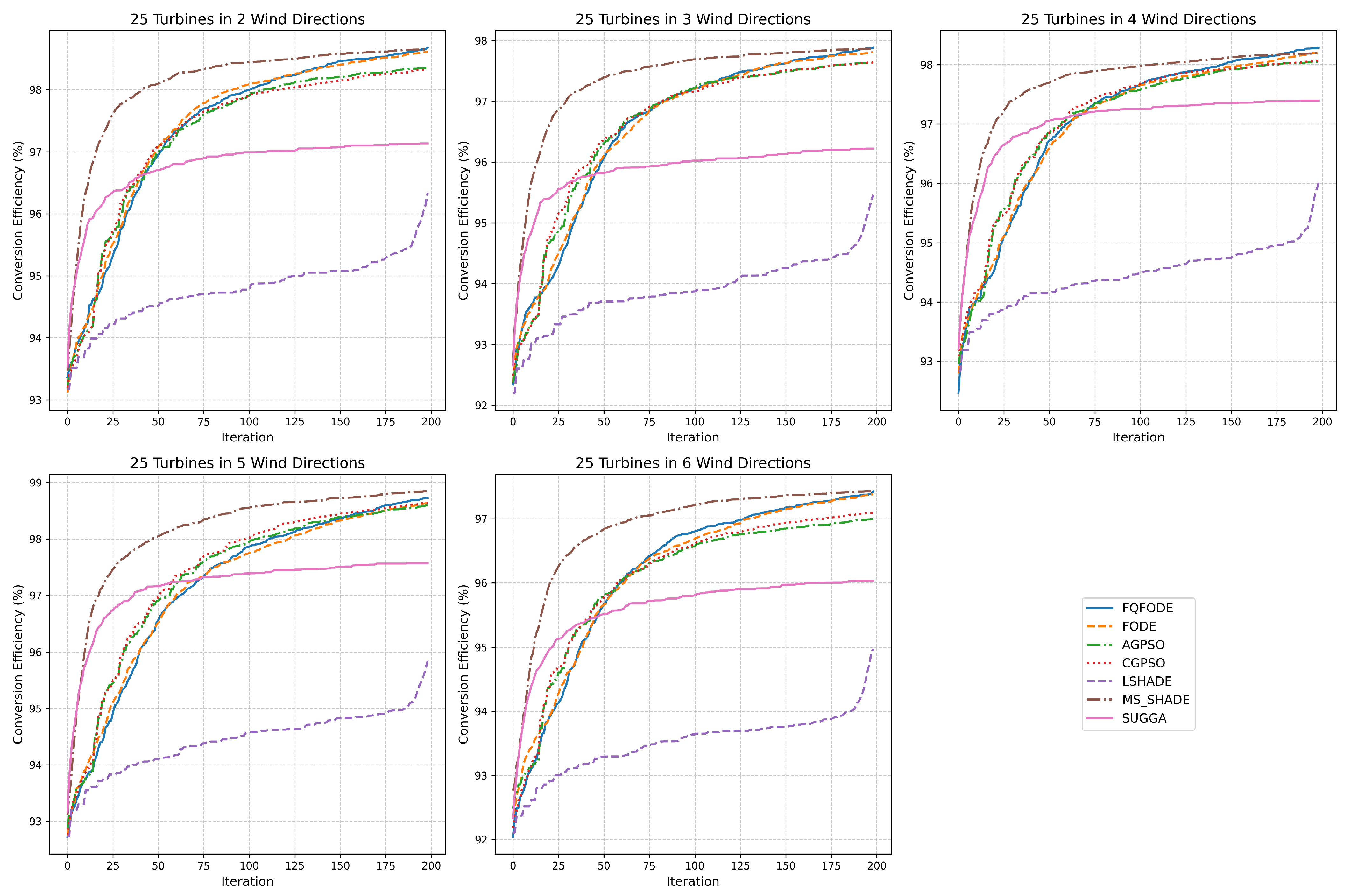
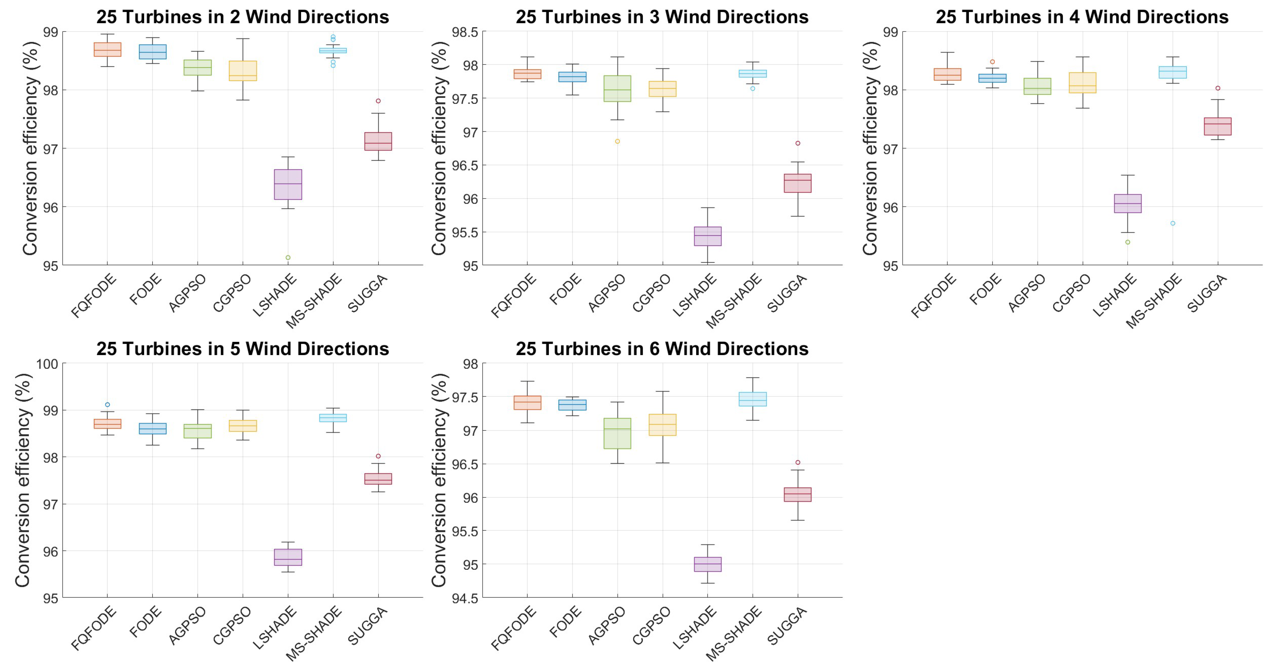
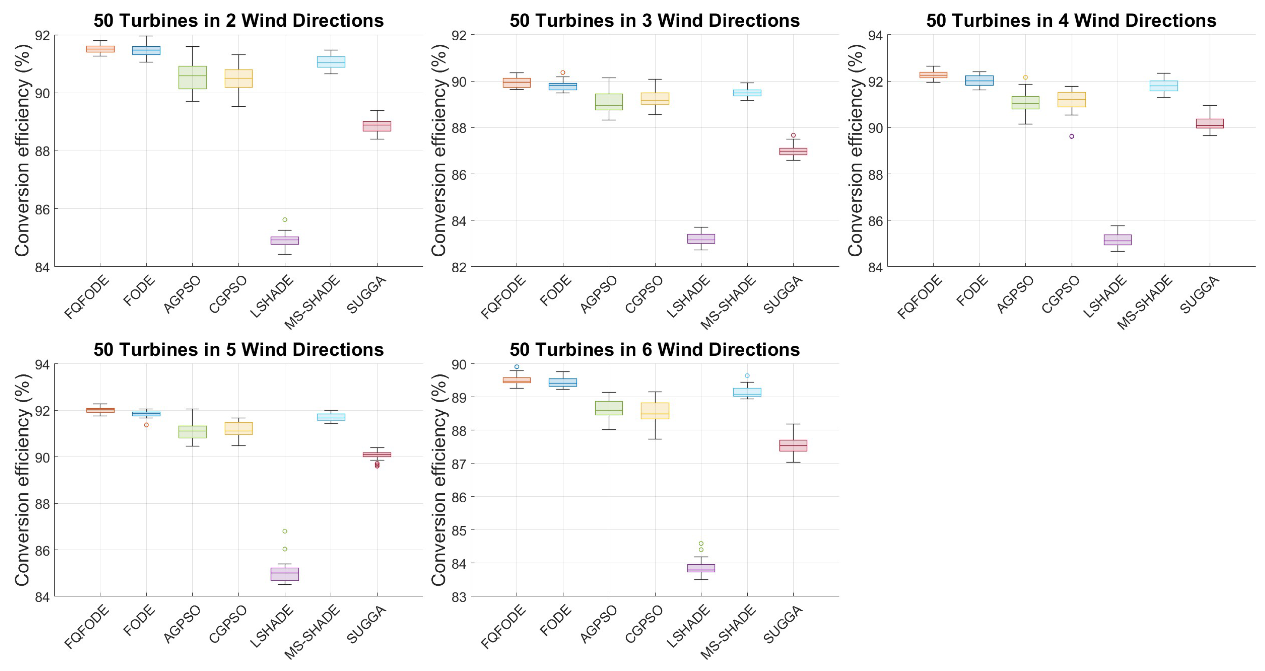
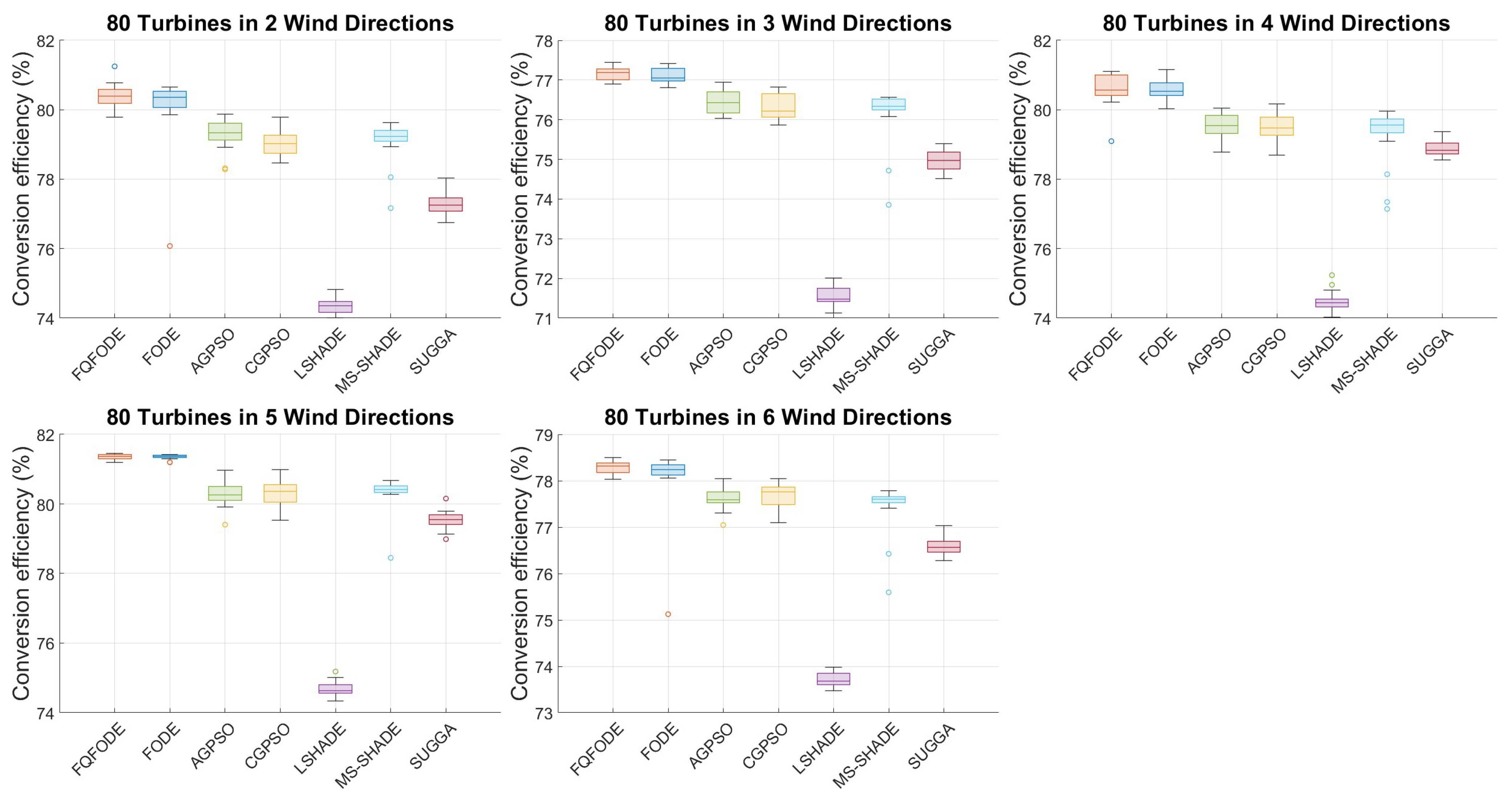
Figure 4, Figure 5, Figure 6, Figure 7, Figure 8 and Figure 9 illustrate the convergence behavior and statistical boxplots of different optimizers under various multi-directional wind conditions. The convergence plots show that in the tn25 setting, FQFODE and MS_SHADE perform comparably in most cases, but FQFODE achieves consistent gains over FODE across all wind conditions, reflecting its greater stability and efficiency during search.

Figure 10 provides a concise visual summary of the win/tie/loss (W/T/L) performance dominance of FQFODE across all comparison cases. It complements the detailed tabular results (Table 5, Table 6 and Table 7) by offering a holistic view of how often FQFODE wins, ties, or loses against each algorithm. This visualization greatly enhances the readability of the extensive statistical data and aligns with recommendations from the reviewers to improve result interpretation. Results are 98.61%, 97.88% vs. 97.81%, and 98.29% vs. 98.20%, respectively; in ws5, 98.73% vs. 98.63%; and in ws6, 97.42% vs. 97.38%. As the problem scale increases to tn50 and tn80, the advantage of FQFODE becomes more stable and pronounced. Compared to MS_SHADE, FQFODE gains approximately +0.45/+0.45/+0.50/+0.36/+0.44 percentage points across ws2–ws6 in the tn50 setting and +1.36/+0.84/+1.09/+1.05/+0.65 in the tn80 setting. Compared to FODE, the improvements are approximately +0.08/+0.10/+0.22/+0.16/+0.07 in tn50 and +0.29/+0.16/+0.16 in ws2, ws3, and ws6 under tn80, with performance nearly identical under ws4 and ws5. These results indicate that in more complex discrete solution spaces, FQFODE not only achieves better final upper bounds and Mean values, but also approaches high-quality solutions with fewer iterations under the same evaluation budget. Compared to FODE and LSHADE-type algorithms, FQFODE leverages its inherited Q-tables obtained through distributed federated pretraining and the stage-wise parameter adaptation mechanism to enhance both global search ability and convergence efficiency in complex scenarios, making it better suited to the discrete structural nature of WFLOP.

In the boxplots shown in Figure 7, Figure 8 and Figure 9, FQFODE consistently shows higher medians, tighter interquartile ranges (IQR), and shorter whiskers, often achieving higher maximum values (upper bounds), which reflects superior typical performance and stronger robustness. For instance, in the tn50 setting, the standard deviation in ws2 is 0.16% for FQFODE compared to 0.20% for MS_SHADE; in ws5, it is 0.14% vs. 0.18%. In tn80 with ws6, the Std is 0.13% vs. 0.26%. From the perspective of “remaining improvement space,” in tn80 under ws2, FQFODE improves from 80.12% to 80.41%, which means it utilizes about 1.46% of the 19.88 percentage point gap from the FODE baseline to the theoretical 100% upper limit—highlighting its refined optimization capacity in later iterations.

Further Insights into Performance, Convergence Dynamics, and Realistic Adaptability

Beyond standard metrics such as Mean, Std, and Best, the performance differences among algorithms can be better understood from three interconnected perspectives: convergence dynamics, solution stability, and robustness to real-world complexities.

(1) Convergence-Speed vs. Solution-Quality Trade-off. As illustrated in Figure 4, Figure 5 and Figure 6, FQFODE demonstrates a distinct two-phase convergence behavior. It initially exhibits fast convergence to rapidly explore promising solution regions and then gradually stabilizes with finer adjustments, leading to high-quality final layouts. This adaptive convergence pattern contrasts with CGPSO and LSHADE, which tend to stagnate early, and with AGPSO, which converges more slowly but less effectively. Such convergence dynamics reflect a typical trade-off: algorithms emphasizing rapid convergence may risk premature stagnation, while overly explorative ones may struggle to refine competitive layouts. FQFODE, through stage-wise Q-learning and historical memory integration, effectively balances these two goals.

(2) Stability and Robustness across Runs. Boxplots in Figure 7, Figure 8 and Figure 9 reveal that FQFODE consistently achieves higher medians, tighter interquartile ranges (IQRs), and lower standard deviations compared to its peers. For example, in the tn80-ws6 scenario, the standard deviation of FQFODE is only 0.13%, versus 0.26% for MS_SHADE and 0.23% for AGPSO. These observations imply that FQFODE produces not only high-performing but also highly stable solutions—critical for deployment in real-world conditions with volatile wind patterns.

(3) Practical Interpretability under Realistic Constraints. Real-world wind farm layouts must contend with fluctuating wind speeds, irregular terrains, and exclusion zones. In such settings, fast convergence may become even more valuable as it enables earlier adaptation to operational constraints. Moreover, solution stability translates to higher robustness against external disturbances. In our experiments, scenarios with larger turbine counts (tn80) and more wind directions (ws6) simulate such complex conditions. In these cases, FQFODE maintains both convergence speed and layout quality. For instance, in WS6tn80, FQFODE outperforms FODE by 0.16% in the Mean and achieves better stability (0.13% vs. 0.64% Std), illustrating its strong adaptability to fragmented, discrete landscapes.

Conclusion. These results collectively highlight that the performance advantage of FQFODE is not merely statistical but structural and functional: it reflects an algorithmic capability to maintain efficient search, adapt to real-world landscape complexity, and reliably deliver high-quality solutions. Therefore, the proposed framework is not only superior in theoretical benchmark terms but also more viable for practical wind farm layout optimization scenarios compared with optimizers that primarily rely on local search; FQFODE’s design—emphasizing global exploration and historical knowledge integration—significantly reduces the risk of premature convergence. Its strong performance in the WFLOP stems from both the non-local search and historical memory characteristics introduced by the fractional-order difference operators in the FODE framework and the dynamic adjustment of the key parameter a via federated Q-learning-based pretraining and stage-wise Q-table control. These capabilities together enable FQFODE to steadily deliver high-quality solutions across complex, multi-directional, and multi-scale discrete optimization scenarios.

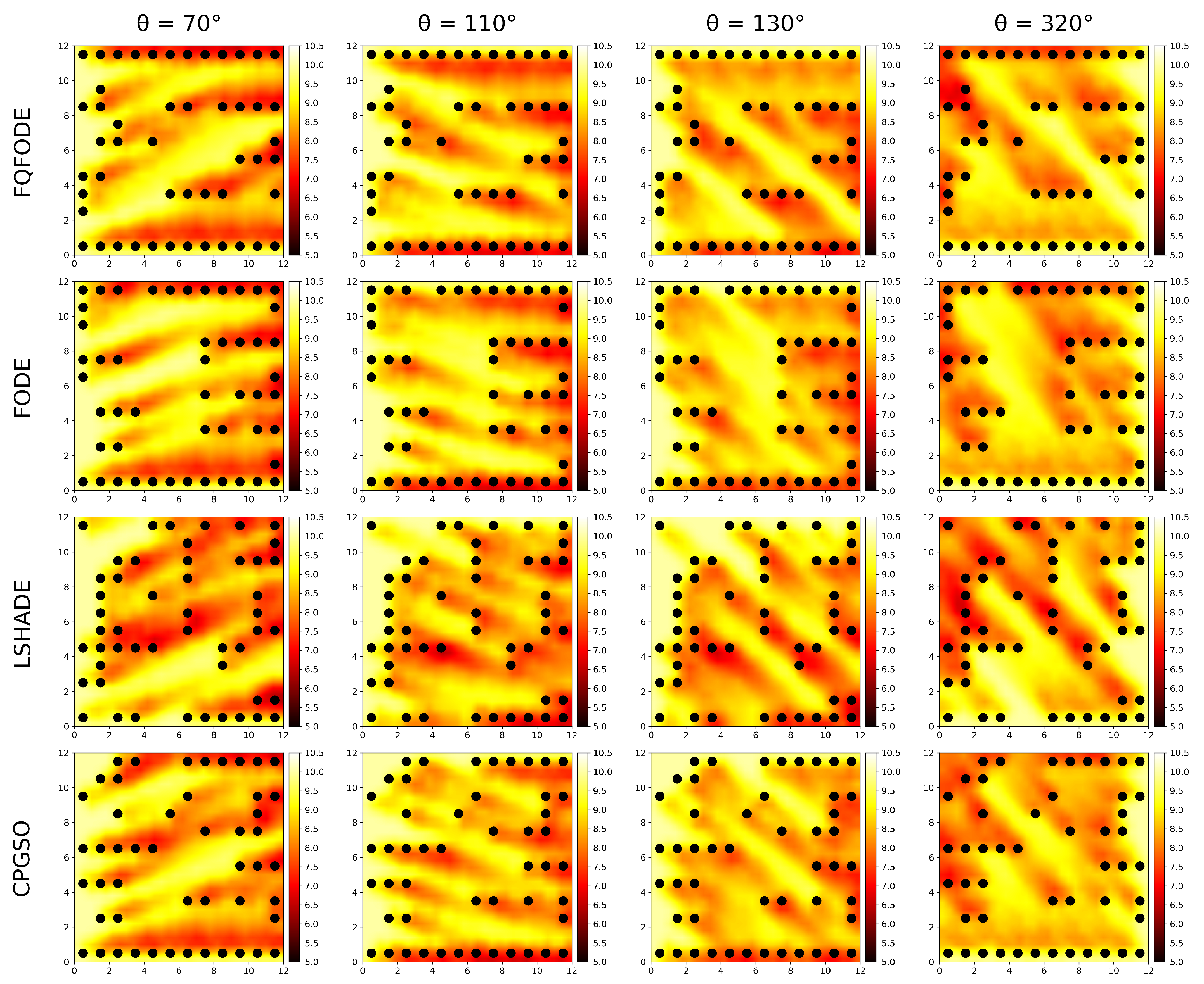
Figure 11 illustrates the turbine layouts produced by four algorithms under four wind-direction conditions for the tn50 scenario, highlighting their adaptability to wake effects. Site discretization. The $12\times 12$ rectangular site is uniformly partitioned into 144 candidate coordinates, each grid cell $(i,j),i,j\in \{1,\dots ,12\}$ corresponding to a potential turbine location. In the figure, black dots denote the discrete coordinates that are actually occupied by turbines, while blank cells remain unused. The background color—from dark red to light yellow—indicates wind-speed intensity (from low to high). The results show that wake interference is primarily concentrated in downstream regions of the turbines, emphasizing the importance of minimizing such interference during optimization. Specifically, the layout generated by LSHADE places many turbines in regions of severe wake overlap, resulting in constrained performance. In contrast, FQFODE arranges turbines in linear patterns along both sides of the wind field, significantly mitigating wake effects. This strategy improves overall power-generation efficiency, underscoring the advantage of FQFODE in wind farm layout optimization.The figure therefore provides an intuitive visualization of the layout–strategy differences across algorithms and offers strong support for understanding the relationship between spatial distribution of solutions and power performance. In this scenario, FQFODE not only achieves a high energy-conversion rate, but also exhibits a more compact, nearly grid-like pattern. This regularity minimizes turbine-to-turbine interference and benefits practical concerns such as installation, maintenance, and efficient land usage. Although algorithms such as AGPSO and CGPSO can also reach relatively high efficiency, FQFODE consistently produces the best solutions with less variation across multiple runs, indicating its robustness in high-dimensional, challenging scenarios.

Overall, these visualization results are consistent with the earlier quantitative analyses based on tables, convergence curves, and boxplots. Whether in simple scenarios where near-perfect solutions are frequently obtained, or in medium-to-high complexity conditions where highly regularized layout patterns emerge, FQFODE consistently demonstrates strong control over the discrete solution space and precise exploration of globally optimal regions. This not only provides further intuitive evidence of its superiority in the WFLOP but also offers a highly efficient and practically implementable layout reference for real-world wind farm design and planning.

3.6. Q-Learning Analysis

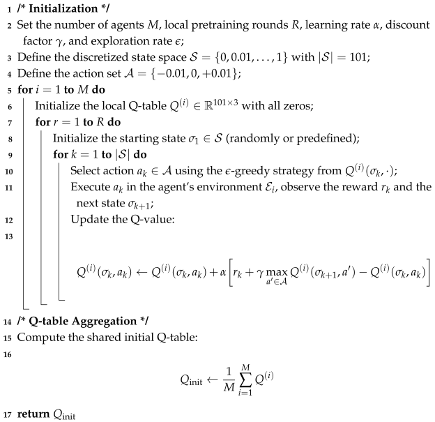
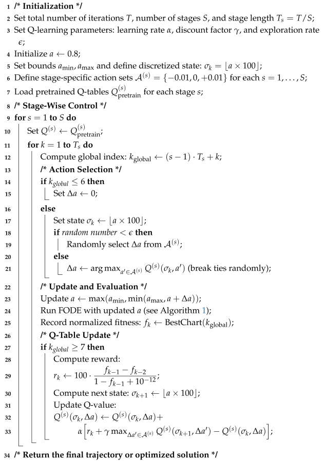
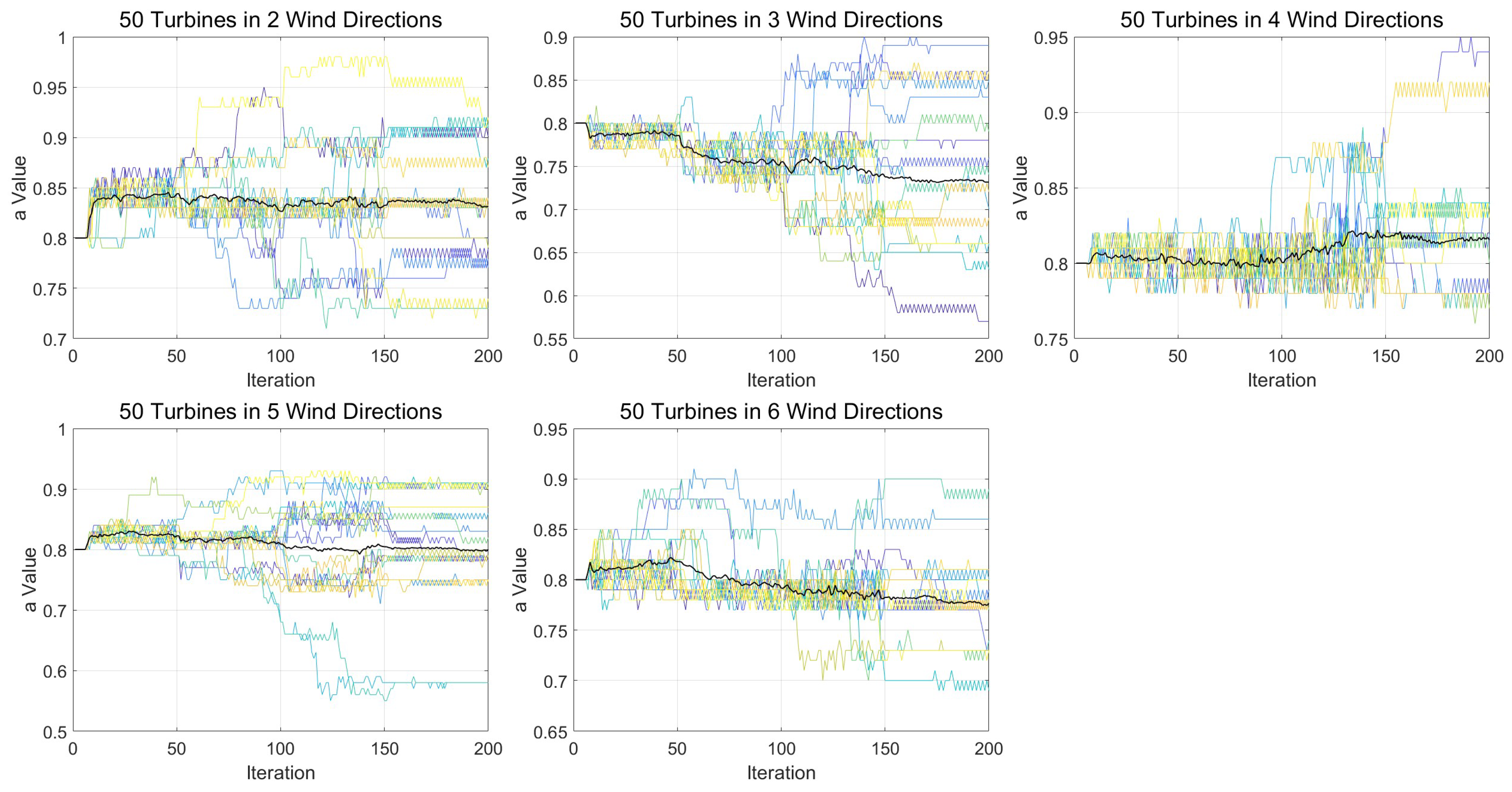
We begin by analyzing the evolutionary behavior of FQFODE across different experiments using the convergence curves of the dynamically adjusted parameter a, as shown in Figure 4, Figure 5 and Figure 6. Each curve in the figure represents one independent run. For each run, the 200 total iterations are divided into four stages of 50 iterations each, corresponding to stage-specific Q-tables (of size 101 × 3) inherited from the distributed federated pretraining. It can be observed that under the same wind condition, the Q-learning mechanism dynamically adjusts the value of the differential weight parameter a based on the current population’s power efficiency and diversity status, thereby implementing an adaptive parameter adjustment strategy that responds to environmental feedback. Due to the differences in early search trajectories caused by distinct random seeds, the early-stage evolution of a may follow different directions. In most cases, significant variations in a occur during the first two stages (iterations 1–100), whereas the later stages (iterations 101–200) show a more stable trend. This indicates that each stage-specific Q-table is capable of independently adjusting a based on the current state and expected return, thereby enhancing the stability and adaptiveness of parameter control.

To further interpret the convergence patterns in Figure 12, Figure 13 and Figure 14, we provide an in-depth analysis of how the dynamic changes in parameter a reflect the internal adjustment strategies of FQFODE. In our design, the value of a determines the extent to which the current generation emphasizes local exploitation versus historical exploration, and its variations over time directly affect the search behavior of the algorithm. Several key trends are observed:

• When a decreases, the influence of current differential vectors weakens, which enhances the mutation’s jump range. This behavior increases global exploration capability, making it easier to escape from local optima.
• Conversely, when a increases, it strengthens the influence of current search directions, encouraging the algorithm to focus more on promising regions. This improves local exploitation capability and precision refinement around high-quality solutions.
• In some cases, a shows a sharp increase during early iterations. This typically occurs when the random initialization produces relatively good solutions, prompting the algorithm to enter a exploitation phase earlier, as early exploitation leads to faster improvement in those scenarios.
• In other cases, a experiences a sudden drop from a high value. This pattern often follows a temporary stagnation phase, indicating that the algorithm attempts to escape suboptimal local regions by reintroducing greater exploration diversity.

These observations collectively suggest that the Q-learning mechanism does not merely adjust a arbitrarily but learns to balance exploration and exploitation based on the current state of the population and feedback from the optimization environment. Such dynamic and context-sensitive behavior enables FQFODE to flexibly respond to different wind farm layout complexities, which is critical for maintaining both convergence quality and search robustness.

To further validate the practical contribution of the proposed Q-learning strategy, we designed a corresponding ablation experiment, and the results are presented in Table 5. In this experiment, the Q-learning module in FQFODE was removed to form the baseline algorithm “NO-QL” (i.e., the original FODE). The results show that FQFODE consistently outperforms NO-QL across all wind conditions and turbine counts, demonstrating the performance-enhancing effect of the Q-learning mechanism. Notably, during the convergence phase, Q-learning not only accelerates the optimization process but also improves the final solution quality. By dynamically adjusting the key parameter a, the strategy strengthens the algorithm’s responsiveness and adaptability across different evolutionary stages, making it a critical factor in achieving efficient search and convergence.

As shown in

Table 8. Comparison of average power generation efficiency with and without the Q-learning strategy across different scenarios (Bold values indicate the winner between the two strategies).

	Methods	TN25	$\mathbf{\Delta }$	TN50	$\mathbf{\Delta }$	TN80	$\mathbf{\Delta }$
WS2	FQFODE	98.68%	+0.0658%	91.51%	+0.0785%	80.41%	+0.2945%
	NO-QL	98.61%		91.43%		80.12%
WS3	FQFODE	97.88%	+0.0749%	89.94%	+0.0954%	77.15%	+0.1604%
	NO-QL	97.81%		89.84%		76.99%
WS4	FQFODE	98.29%	+0.0855%	92.27%	+0.2200%	80.60%	+0.0009%
	NO-QL	98.20%		92.05%		80.60%
WS5	FQFODE	98.73%	+0.0962%	92.02%	+0.1575%	81.36%	+0.0029%
	NO-QL	98.63%		91.86%		81.36%
WS6	FQFODE	97.42%	+0.0395%	89.53%	+0.0634%	78.29%	+0.1579%
	NO-QL	97.38%		89.46%		78.13%

, FQFODE consistently outperforms the NO-QL baseline across all wind conditions and turbine configurations. Bold values indicate the winner between the two strategies.

It is worth noting that although the average improvement in power efficiency brought by the Q-learning mechanism appears modest—approximately $0.2945\%$—its practical significance in large-scale wind farms is substantial. Take, for example, a typical wind farm with 80 turbines (each rated at $3.6\mathrm{MW}$ and with an annual capacity factor of $32.3\%$), which yields an estimated annual power generation of $8.16\times {10}^8\mathrm{kWh}$. Based on this estimate, the efficiency improvement translates into approximately $2.40\times {10}^6\mathrm{kWh}$ of additional electricity per year—equivalent to around 2.4 million kilowatt-hours. Assuming an average industrial electricity price of $0.4\mathrm{CNY}/\mathrm{kWh}$ in mainland China, this would yield an additional annual revenue of approximately 960,000 CNY. Referring to typical European onshore wind electricity prices (e.g., EUR $0.08/\mathrm{kWh}$), the corresponding annual revenue increase could reach approximately EUR 192,000. This clearly demonstrates that even seemingly small improvements in efficiency can lead to substantial economic value in real-world systems.

4. Conclusions

The proposed FQFODE algorithm demonstrates superior performance over the original FODE in solving the WFLOP under various realistic wind conditions. In a comparative evaluation against six state-of-the-art optimizers across 15 experimental scenarios, FQFODE achieved a win rate of up to 92.2% (83 wins/6 ties/1 loss). In the direct comparison with FODE, FQFODE consistently improved the average energy conversion efficiency under all test conditions, with a maximum gain of 1.46%. Furthermore, in large-scale, multi-directional layout problems, the turbine arrangements generated by FQFODE exhibit more regular structures and stronger engineering applicability, offering more rational land-use strategies for wind farm construction and subsequent operation and maintenance. From a structural design perspective, FQFODE integrates inheritance-based Q-tables—generated through multi-round pretraining—with the fractional-order difference mechanism from FODE and incorporates a stage-based parameter adjustment strategy to dynamically adapt the critical control parameter a. Specifically, the optimization process is divided into two phases: In the first phase, federated Q-table aggregation enhances the knowledge transfer capability of the Q-learning strategy across multiple agents, overcoming the limitations of single-path training. In the second phase, during the formal optimization process, the parameter a is dynamically adjusted based on environmental feedback in a stage-wise manner, enabling fine-grained exploration and local exploitation in high-dimensional search spaces. In contrast, the original FODE uses a fixed fractional memory factor and lacks adaptiveness to complex and variable wind conditions, limiting its optimization flexibility. Experimental results further verify the advantages of FQFODE. In representative WFLOP tests involving 25, 50, and 80 turbines, FQFODE outperforms FODE in multiple dimensions: it not only significantly accelerates convergence—requiring fewer iterations to reach equivalent performance—but also improves the final average power output by approximately 0.12%. Moreover, under non-uniform wind conditions, FQFODE exhibits greater solution stability, with an average reduction of 7.97% in standard deviation. These comparative results fully validate the synergistic effectiveness of the federated pretraining and stage-wise parameter control strategies within the differential evolution framework. They also highlight FQFODE’s strong potential for application and further development in complex discrete optimization problems such as the WFLOP.

4.1. Limitations and Future Improvements

Despite its promising results, FQFODE still exhibits certain limitations that warrant further investigation. First, we observed that the performance advantage of FQFODE over baseline methods becomes less pronounced in relatively simple scenarios with low problem complexity. This is likely because most algorithms—including CGPSO and FODE—can rapidly converge in such settings, and the long-term benefits of reinforcement learning are not fully utilized during the short convergence process. Second, while CGPSO performs robustly in low-dimensional or structured search spaces, its performance degrades significantly in more complex scenarios, where FQFODE demonstrates superior adaptability. Regarding the comparison with FODE, it is important to note that FODE itself leverages a historical-difference-driven evolution mechanism, making it a strong baseline. In a few test cases, FQFODE and FODE show similar performance, possibly due to individual initialization bias or the Q-learning policy not being fully activated. Moreover, there remain technical aspects of FQFODE that can be improved. (1) The current four-stage learning schedule is equally partitioned in terms of iteration count (e.g., four 50-generation stages), rather than being dynamically determined based on actual convergence behavior. Future work may involve analyzing large-scale optimization trajectories to establish adaptive phase boundaries that better align with the optimization process. (2) The current reward function applies normalized improvement metrics. However, due to differences in problem scales (e.g., 25-turbine vs. 80-turbine cases), the absolute range of objective values varies significantly, potentially causing reward inconsistency. We aim to investigate segmented normalization or guided reward shaping strategies to enhance the generalization and learning stability of the Q-tables. These refinements will help further enhance the adaptability of FQFODE in more diverse WFLOP scenarios.

4.2. Future Work

Building upon the identified limitations of the current FQFODE algorithm, future research can proceed along several directions to further deepen and broaden this study. On the algorithmic side, we plan to improve the generalization and convergence efficiency of FQFODE by refining its stage partitioning strategy and reward function design. Specifically, this includes dynamically determining phase boundaries based on real-time convergence trajectories and constructing reward scaling mechanisms with consistent normalization across different problem sizes. These enhancements are expected to improve the responsiveness and learning stability of the Q-table-based policy. Furthermore, adaptive Q-learning strategies will be explored, such as dynamically adjusting the exploration rate ($ϵ$) or learning rate ($\alpha$) according to convergence trends. This is expected to enable the Q-controller to better adapt to the complex and evolving search environment.

In addition, we plan to investigate the integration of advanced deep reinforcement learning methods (e.g., DQN; Actor–Critic) into the evolutionary mechanism. Such extensions could further enhance the algorithm’s decision-making capability and provide a richer control policy. Meanwhile, the core mechanisms of FQFODE can be extended to other challenging combinatorial optimization problems, such as multi-objective wind farm layout planning or hybrid wind–solar site selection, to verify the adaptability and scalability of the proposed framework beyond the current WFLOP context.

We also aim to evaluate FQFODE under more complex wind field models, including seasonal wind variation, terrain-induced disturbances, and three-dimensional wind distributions, to bring the algorithm closer to real-world engineering conditions. Given the current scarcity of high-fidelity public datasets for such tasks, we hope to collaborate with industry partners to jointly develop more advanced testing platforms and representative wind farm benchmarks. Finally, we will promote the open-source release of FQFODE code and data to facilitate reproducibility, community-driven improvements, and real-world deployment, contributing to a more transparent and collaborative environment for WFLOP research and optimization algorithm development.