Abstract
Fractal dimensions for the daily discharge data series of several karstic springs in northeast Hungary have recently been computed and analyzed. We model four of those series with similar fractal dimensions using a superposition of a fractional Ornstein–Uhlenbeck process and a jump process of renewal–reward type. Beyond some usual goodness-of-fit measures, simulations of the model show an visually appealing good fit. When the fractal dimension is not taken into account in the modeling, the simulated accumulated discharges tend to significantly exceed realistic values.
Keywords:
fractal dimension; karstic aquifer; fractional Ornstein–Uhlenbeck process; jump process; renewal–reward process MSC:
60G22; 60G55; 60K15; 62M10; 86A05
1. Introduction
Karst spring discharge time series are known to exhibit highly irregular, heterogeneous, and multifractal dynamics [1,2]. These complex patterns reflect the underlying geologic heterogeneity, including the interaction between the porous matrix, fracture networks, and conduit systems [3]. Traditional linear hydrological models, which often rely on simplified assumptions of stationarity and Gaussian-like fluctuations, fail to capture the intricacies inherent in karst hydrology, such as long-range dependence, sudden jumps in flow rates, and the influence of extreme events [4].
The recession curves of karst spring hydrographs, frequently decomposed into distinct flow components (e.g., conduit-driven quick flow and matrix-driven base flow) serve as important indicators of aquifer properties, infiltration processes, and hydraulic connectivity [1]. Although conceptual models such as those proposed by Mangin [5] and Fiorillo [1] provide useful insights by distinguishing various storage and drainage compartments, they often lack the ability to represent the non-linear and fractal or multifractal nature of observed discharge records [2,5]. Empirical studies have shown that karstic systems display scale-invariant behavior: the complexity of flow paths and conduit geometries induces fractal patterns in spring discharge time series [6]. The fractal dimension (D) characterizes the degree of roughness and complexity on multiple scales [7,8] and, thus, serves as a crucial quantitative measure to understand karst processes [9,10].
Moment scaling for several springs, including the ones that are the subject of the present study, was presented in [10] indicating that most hydrographs are monofractals rather than genuine multifractals (cf. [11], section 6.3). Hence, a single number for the fractal dimension is fully informative. Theoretically, box-count and information dimensions coincide for monofractals; therefore, they similarly characterize the springs. As a result, the information dimension does not provide valuable new information but strengthens that of the box-count (capacity) dimension, which we consider throughout the present study.
Motivated by these findings, our primary objective here is to develop a stochastic modeling framework capable of reproducing both the fractal scaling and the jump-like features observed in karst spring discharges. In this study, we employ a fractional Ornstein–Uhlenbeck process (fOUp) enriched with jump components to model and simulate karst spring discharge dynamics. The fOUp is a continuous-time Gaussian process with long-range dependence characterized by a Hurst exponent (H, with ), allowing it to capture persistent () and slowly decaying autocorrelations or anti-persistent (), rough fluctuations inherent in karst systems [12].
The usual, mean-reverting Ornstein–Uhlenbeck process (OUp; ) is defined by the stochastic differential equation (SDE):
where is the mean reversion parameter, is the long-term mean, is the volatility, and is a classic Brownian motion. Extending the OUp to a fractional context involves replacing with a fractional Brownian motion () of the Hurst index (H). This introduces long-memory characteristics into the dynamics when and rough fluctuation when .
The ultimate source for renewing the karstic hydrogeological system is infiltration from precipitation or from melting snow. To address sudden discharge spikes originating from infiltration, we incorporate a jump component into the driving force of the fractional Ornstein–Uhlenbeck (fOU) equation, resulting in a hybrid model that can be schematically written as follows:
where represents the jump component. In general modeling practice, the jump component () often follows a compound Poisson process. However, a shortcoming is that the jump times and jump sizes are independent, and the process includes the Markov property, enforcing exponential interarrival times (i.e., times between jumps, also called sojourn times in renewal theory). This property is counterintuitive in our application, since a long delay between jumps—induced mainly by long delays in precipitation events—leaves the aquifer drained. Hence, the water from the next precipitation event—or a quick snowmelt for its turn—is kept back in the aquifer, filling up the porous matrix and the fracture networks, allowing for only lesser peaks in spring water discharge. Inspired by renewal theory and supported by statistical evidence (see Section 6), we suggest using a semi-Markov jump process for with Weibull-distributed interarrival times and Weibull-distributed peaks [13]. In hydrology, the two-parameter Weibull (EV Type III) distribution is well known to fit low-flow and spring-flow extremes. For example, Sugiyama et al. (2007) [14] noted that ”the Weibull distribution is very suitable for the probability plot of low stream flows”. Likewise, in our context, Leone et al. (2021) [15] found that fitting spring discharge with a Weibull distribution ”fits the extreme values of both tails well”. Furthermore, a physical rationale is that the interarrival times between flow pulses can be viewed as “time-to-threshold” or “time-to-failure” processes (analogous to reliability theory), for which Weibull laws often arise. Contrary to Markov models, semi-Markov models allow for interdependence of the process state and the interarrival time and essentially place no restriction on the interarrival time distribution (see, e.g., ref. [13]). The proper correlation of the interarrival times and the jump sizes is secured by the probability integral transform and its inverse, along with the Gaussian copula. To the best of our knowledge, this model specification is novel in the literature. The jump component describes the abrupt short term, whereas the fractional component fine tunes the long-term behavior.
We apply this fractional jump Ornstein–Uhlenbeck framework to daily discharge data from karst springs in northeast Hungary. The associated analysis illustrates the methodology’s capacity to replicate both the statistical and scaling features of the observed time series. By comparing simulated and observed discharge data, we demonstrate that this modeling strategy can reproduce essential empirical characteristics, such as fractal scaling, non-Gaussian tails, and sudden discharge extremes. Thus, the jump–fOUp approach provides new insights into the structure and complexity of karst aquifers and represents a promising avenue for understanding and predicting the non-linear, non-stationary, and fractal-like behavior of karstic spring discharges.
The remainder of this article is organized as follows. Section 2 introduces the modeling framework—a fractional Ornstein–Uhlenbeck process augmented by a renewal–reward jump term—together with its mathematical properties and a short proof of its well posedness, which can be found in Appendix A. Section 3 reviews existing estimation techniques for the pure fOU process and adapts them into a two-tier procedure that later underpins our jump–fOUp inference. Section 4 describes the geological setting, the 19-year daily discharge dataset from four Hungarian karst springs, and the exploratory analyses that motivate our model choices. Section 5 presents the complete estimation–simulation workflow: detection of surges, copula-based generation of correlated jump pairs, fGn simulation for the fractional kernel, and the iterative scheme that couples both components. Section 6 compares observed and simulated hydrographs, fractal dimensions, and cumulative discharges, demonstrating that jump–fOUp reproduces key statistical and visual features markedly better than short-memory alternatives. Section 7 discusses hydrological implications, the necessity of long-range dependence, and possible extensions, such as time-varying parameters or precipitation-driven jump intensities. Finally, Section 8 concludes with the main findings and outlines directions for future research.
2. Fractional Ornstein–Uhlenbeck Process with Renewal Jumps
2.1. The Pure fOUp
The (mean-reverting) fractional Ornstein–Uhlenbeck process (fOUp) extends the usual Ornstein–Uhlenbeck model by incorporating the fractional Brownian motion (fBm) as its driving noise term. To distinguish it from its jump-enriched counterpart, we refer to it as pure fOUp. The fractional Brownian motion generalizes the classic Brownian motion () to incorporate long-range dependence or rough paths. If , the increments are positively correlated, leading to persistent behavior, i.e., long memory. If , the increments are negatively correlated, resulting in rough paths and antipersistent behavior. Let be a continuous-time stochastic process satisfying the stochastic differential equation (SDE):
where is the mean reversion rate, is the long-term mean toward which reverts, is the volatility parameter, and is a fractional Brownian motion with Hurst parameter . The solution of the fOU equation exists is unique up to initial condition . It can be expressed as follows [12]:
For , the fOUp reduces to the usual OUp driven by a classic Brownian motion. The long-memory or rough path behavior is inherited by the fOUp from fBm according to the Hurst parameter. Unlike Bm and fBm, the fOUp has a stationary regime. In contrast to the usual OUp, the fOUp is non-Markovian for . For more details on the fOUp see, e.g., ref. [12].
2.2. Adding Jumps to the fOUp
We extend the fOUp dynamics by including jumps in the driving force to capture the long-memory or rough behavior of hydrological processes alongside sporadic, strictly positive surges that can be extreme in magnitude. The fOUp component encodes persistent correlations or rough fluctuations observed in hydrology. The jump components are responsible for the shocks that arrive from extreme water infiltration. In the simplest analog, the jump diffusion setting, one might add a compound Poisson process whose interarrival times are exponentially distributed and whose jump sizes can, in principle, have arbitrary distributions. However, in hydrological systems where only positive, heavy-tailed surges are relevant and where jump sizes and interarrival times can exhibit dependence, the assumption of a compound Poisson structure becomes too restrictive. Our approach uses an analogy to renewal theory and incorporates an additive renewal–reward term into the fOU equation.
We enrich fOUp with jumps by first specifying a renewal–reward process (). The process () is specified by a sequence of increasing jump times ( with ). The interarrival times ( ) are positive, random variables, and the jump sizes () are positive, random variables. We set . With these if . Both interarrival times () and jump sizes () have a Weibull distribution in our application, and the and variables are correlated. In this way, is a point process, with a non-decreasing, right-continuous, step-function sample path structure, for which stochastic integrals can be defined in terms of standard Lebesgue–Stieltjes integration theory. As a result, its differential can also be viewed as a stochastic measure that puts jump-size weights () on jump-time points (). Now, we define our jump–fOUp process () as follows:
Theorem 1.
Let be defined by Equation (5). Then, satisfies the stochastic differential equation:
where is the mean reversion rate, θ is the equilibrium level, is the volatility, is a fractional Brownian motion (same as used in Appendix A—standardized notation to ), and is the renewal–reward process defined above.
We present the proof of the theorem in Appendix A.
The jump term () accumulates at random times governed by Weibull-distributed interarrivals and delivers jump magnitudes that are also Weibull-distributed. This construction ensures that each surge contributes a strictly positive, heavy-tailed (as the Weibull shape is invariably less than one in these applications; see Section 6) increment to and that the negative correlation of interarrival times and jump sizes is preserved. The semi-Markov property emerges because the distribution of waiting times until the next jump depends on previously realized jump sizes (and vice versa), thereby departing from the memoryless exponential interarrivals of a compound Poisson process.
The flexibility of the model, resulting from the semi-Markov construction, allows for the simultaneous reproduction of heavy-tailed surges and their further spreading effect and long-memory fluctuations. This resolves a common challenge in hydrological modeling, where only positive, subexponential jumps with significant extremal impact can occur. By merging Weibull-based jump processes with fractional diffusion, one captures rare yet sizable excursions on top of a persistently correlated or anti-persistent baseline.
3. Parameter Estimation Methods
Much effort has been devoted to the parameter estimation problem for fOU processes. Assuming that a continuous record of observations is available in the non-mean-reverting case (), Kleptsina and Le Breton [16] were the first to obtain the formula for the estimation of the drift parameter’s maximum likelihood (ML) and proved almost sure convergence. Bercu, Courtin, and Savy [17] proved a central-limit theorem for the MLE in the case of . They claimed, without proof, that the above convergence is also valid for . Finally, Tanaka et al. [18] completed the case by studying ML estimates when and .
Turning to mean reversion with and keeping the assumption of continuous observation, Lohvinenko and Ralchenko [19] obtained ML estimates of and when and .
Estimating the parameter vector () of the fOUp in the more realistic case of discrete, time-equidistant observations () poses significant challenges due to the fractional nature of the driving noise. In the non-mean-reverting case, specialized statistical methods were developed in [20,21], using the relationship between the Skorokhod (or divergence) and Stratonovich integrals. These works also provide limit theorems for the estimation, as both the time horizon and the mesh size grow to infinity simultaneously and the horizon increases faster than the mesh size. However, this condition is difficult to verify in a real application with a finite sample size.
3.1. A Two-Tier Estimation Framework for the fOU Parameters
This section consolidates, in a single presentation, the continuous-record methodology of [20,21] and its exact, discrete-sample analog introduced in [22]. Both procedures target the parameter vector () of a fOUp.
3.1.1. Tier I—Continuous Record (Ref. [21])
Assuming full observation of the path (), the mean reversion speed () can be consistently recovered by either least squares, i.e.,
or the energy-type statistic, i.e.,
where denotes Euler’s gamma function. Both estimators are strongly consistent and asymptotically normal as .
3.1.2. Tier II—Exact Discrete Record (Ref. [22])
Let be an equally spaced sample of size N with a grid step of . We define second-order differences and their quadratic variations.
Closed-form, strongly consistent estimators are then obtained as
4. Application to Karstic Spring Discharge Modeling
4.1. Geological and Hydrological Settings
The Aggtelek Karst, part of the Gömör-Torna Karst region on the Hungarian–Slovakian border, is predominantly composed of Triassic carbonates, mainly Wetterstein limestone and dolomites [23]. The Hungarian section comprises approximately 200 km2 of east–west-oriented karst plateaus at elevations of 400–600 m a.s.l., dissected by valleys as low as 150–260 m. Karstification began in the Miocene under subtropical conditions, with significant Pliocene uplift that forms the present-day north–south topographic gradient [24,25]. The mean annual precipitation is about 600 mm, most of which infiltrates the plateau and resurfaces at karst springs. The area has a humid continental climate with a mean annual temperature of 9.1 °C, about 120–130 frost days, and 40 snow-covered days annually [23].
These geological and climatic data originate from Telbisz et al. [23]. The dataset and descriptions therein are based on decades of multidisciplinary fieldwork and geological mapping [26,27] and are considered reliable and high-quality within the regional geoscientific community.
4.2. Data Description
The measurement of the daily spring discharge of the most significant karstic springs in the Aggtelek Karst was carried out by the Hungarian Water Resources Research Plc. (VITUKI) from the early 1960s to the 1990s [28]. We selected four springs (Csörgő, Kecskekút, Komlós, and Lófej) with non-missing daily observations for 6200 days in the period from 1 March 1974 to 18 February 1993. The basic descriptive statistics of these decades of uninterrupted hydrological data series are shown in Table 1.

Table 1.
Characteristics of the four selected springs: aquifer size, daily average discharge (Q), ratio of maximum to median discharge (), coefficient of variation (CV) for discharges, and water temperature statistics.
The springs are located within a relatively small area, close to each other (Figure 1). However, significant scale differences can be observed in their daily discharges: the multiannual averages vary between 287 and 14,508.5 m3/day (see Table 1). Cave systems of varying lengths are known to be connected with the springs [29,30]. In Jósva, spring water comes to the surface from the 25 km long Baradla-Domica cave system. Komlós spring (Kom) is connected to Béke cave (approx. 7.2 km long). Szabadság cave (approx. 3.2 km) belongs to the aquifer of Kecskekút spring (Kec). Caves of much shorter confirmed lengths—typically a few hundred meters, as reported to date by cave researchers—lie behind the Csörgő spring (Cso) [29]. The cave systems direct quick flows to the mouth of the springs, playing an essential role in shaping the surges in the hydrographs.
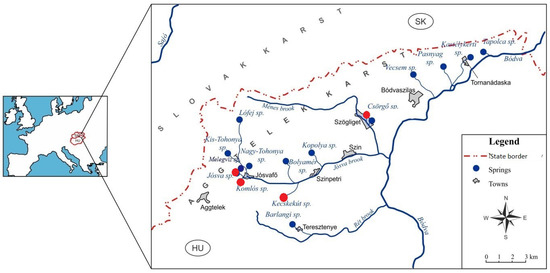
Figure 1.
A schematic map displaying the location of the four selected springs in the Aggtelek Karst region, NE Hungary. Red figures highlight the location of springs, subject to the present study.
5. Methodology: Parameter Estimation and Simulation
The objective is to model the daily discharge time series () of several karst springs. The model assumes that the discharge dynamics result from the superposition of a continuous, persistent background process and discrete, sudden jump events, often triggered by precipitation. A jump–fOUp, as described in Section 2, is employed. The analysis proceeds spring by spring; the following sections outline the methodology for a single representative time series (, where ). The modeling process involves two main phases: estimating model parameters from the observed data and simulating the process using these parameters.
5.1. Phase 1: Parameter Estimation from Observed Data
5.1.1. Data Preparation and Initial Analysis
Let denote the observed discharge at day t. The differenced series ( for ) is calculated to highlight rapid changes or jumps (Algorithm A1, line 1).
5.1.2. Jump-Component Identification and Characterization
- Jump Detection: Jumps are identified where exceeds a high quantile threshold of , where p is a high probability, chosen as 0.975 (Algorithm A1, line 2). Let be the time index of the j-th detected jump (; Algorithm A1, line 3). For a heuristic explanation, see Section 6.1.
- Jump Size Analysis: The jump sizes are (Algorithm A1, line 4). Their distribution is analyzed by fitting candidate distributions (Weibull and Gamma) to using Maximum Likelihood Estimation (MLE) (Algorithm A1, lines 6). Goodness of fit is assessed using Kolmogorov–Smirnov (KS) tests. Let denote the estimated jump-size parameters.
- Jump Timing Analysis: The interarrival times (, where ) are calculated (Algorithm A1, line 5). Their distribution is analyzed similarly, fitting a Weibull distribution to slightly perturbed data via MLE (Algorithm A1, line 8). Perturbation is necessary because, as a continuous distribution, integers and ties do not fit the Weibull distribution. Perturbation is created by adding a uniform [0.01,0.5] variable to the jump sizes. The effect of the perturbation is then analyzed using 100 perturbations. Let denote the estimated jump-time parameters.
- Jump Dependence Structure: The dependence between jump sizes () and preceding interarrival times () is quantified by the sample correlation coefficient (; Algorithm A1, line 9). Typically, is significantly less than 0.
5.1.3. Background Process Characterization
- Hurst Parameter Estimation: The long-range dependence is quantified by the Hurst parameter (). According to the model assumption, after the jump-filtering step, the residual series behaves as a fractional Ornstein–Uhlenbeck process; hence, we may use the well-studied second-difference (or energy-type) estimator (9) (Algorithm A1, line 10) that is consistent and asymptotically efficient for fOUp paths [17,20,21,31]. This estimator assumes a continuous-path Gaussian driver and would be biased if applied to a series containing discontinuous jumps. Therefore, for the full discharge record, the complete process with jumps (9) is not applicable. In this case, we rely on the more universal madogram-based fractal dimension estimator (). With that, the Hurst parameter is estimated as , which is robust to discontinuities and does not require Gaussian increments. It also serves to remain compatible with the findings of [10].
- Fractional Ornstein–Uhlenbeck (fOU) Parameter Estimation: The background process is modeled as an fOUp, and its parameters are estimated from a truncated series (); Algorithm A1, lines 11–12; see also Section 6).
- –
- Volatility (): Estimated from the second differences of using :(Algorithm A1, line 13).
- –
- Mean Reversion Rate (): Estimated from the variance of and :(Algorithm A1, line 14).
5.2. Phase 2: Simulation Setup
- Jump Simulation via Gaussian Copula: To preserve the empirically observed negative correlation () between jump sizes and interarrival times, we employ a Gaussian copula. This construction uses the probability-integral transform and a normal copula to generate correlated samples. We chose the Gaussian copula because it is simple and adequately models the moderate correlations (– in our data) without introducing additional tail dependence. Other copulas could be used, but in terms of correlation, the Gaussian copula reproduces the joint behavior of surge pairs well. Note that the relatively small number of jumps makes addressing tail dependence between jump size and interarrival time—and, thus, choosing a heavy-tailed copula—difficult, if not arbitrary. For comparison, Kalantan & Abd Elaal (2018) [32] evaluated Gaussian–copula Weibull models with synthetic sample sizes of , while Ahmed et al. (2021) [33] studied tail dependence in Archimedean–copula Weibull pairs only for ; our empirical dataset (∼150 jumps per spring) falls below that threshold, rendering a reliable tail-dependence fit impractical. Accordingly, we do not fit Archimedean or t-copulas whose main advantage is tail dependence. Given the moderate observed dependence and limited sample sizes, the Gaussian copula is a pragmatic and sufficient choice for our purposes.To create a large sample from the Gaussian copula, pairs of correlated standard normal variables with correlation () are generated and transformed to uniform via the normal CDF (Algorithm A1, line 15–16). Simulated interarrival times () and raw jump sizes () are generated using the inverse CDFs of the fitted Weibull distributions (Algorithm A1, lines 20–29). Since this transformation does not preserve the correlation, is set slightly larger than , the target parameter. Subsampling is then performed on these L pairs until we obtain a final sequence of pairs —so many that jump times cover the [0,T] time interval and their correlation reaches the target (Algorithm A1, lines 19–25). An innovation array () of length N is built by filling it up with the final jump increments () at the simulated jump times (), with zeros elsewhere. (Algorithm A1, lines 31–34).
- Fractional Gaussian Noise (fGn) Simulation: A sequence of fGn increments () with the Hurst parameter () is generated by differencing a simulated fBm (e.g., by using the somebm package of R) and scaled using the estimated volatility (; Algorithm A1, lines 36–37).
5.3. Phase 3: Combined Process Simulation Loop
Writing as and integrating it in (5), first from 0 to , then from to t, we obtain
The last integral is if for a jump time of or zero otherwise. Since is small in our case, we obtain an approximation:
Using the approximation, the discretized discharge series () is generated iteratively for :
where is the total innovation, the sum of the jumps, and the scaled fGn, and is the initial value (Algorithm A1, lines 38–42).
This procedure generates a synthetic time series () to replicate the statistical properties of the discretely observed discharge.
6. Application: Jump Distribution Fitting and fOUp Parameter Estimation for Karstic Spring Discharges
6.1. Separating the Jumps
The surges in spring discharges are not merely isolated spikes; rather, they exert a dampening effect on the recession curve. Consequently, it is not sufficient to model these as simple jumps in the process itself—they must be incorporated into the driving force of the dynamics, specifically in the differential component of the stochastic differential equation (SDE). Therefore, to locate the jump positions and sizes, the differenced series has to be considered. The quantiles and maxima of the differenced spring discharge series are presented in Table 2.
Table 2.
Quantiles and maxima of differenced spring discharge series (m3/day).
The comparison of quantiles, maxima, and their relative proportions in Table 2 reveals the heavy-tailed nature of the underlying distribution. This observation rules out the adequacy of a pure fOUp for modeling. Replacing fractional Brownian motion (fBm) with a Lévy flight in the SDE could address heavy-tail behavior, but it would fail to capture the correlation between extreme values and their timing. This limitation motivated the development of our proposed approach.
To corroborate the jump threshold used in this study, Table 2 lists the empirical , , and quantiles. Across all springs, the largest observed surge is roughly 20 to 450 times the quantile and 10 to 200 times the quantile, while the quantile is only 2 to 3 times the quantile. So, choosing the quantile level as the cut-off effectively separates the extreme outliers, interpreted as hydrogeological ’jumps’, from the long-memory background. A total of 155 values are observed above the quantile level, and it is still suitable to fit a distribution to them with sufficient accuracy. Hence, we choose this threshold to determine the jumps.
6.2. Jump Distributions and Waiting-Time Dependence
We analyze karst spring discharges through two complementary layers. First, we model the jump component by semi-Markov dynamics, whose interarrival times and magnitudes follow Weibull laws. Jump parameters (interarrival time and jump size distributions) were fitted by maximum likelihood and validated—for jump size, against a gamma distribution, too—with Kolmogorov–Smirnov tests reported in Table 3. In addition, we compared Weibull fits to alternatives (e.g., gamma and log-normal) and found Weibull giving the lowest AIC and the most balanced fit to small and large flows. We report these statistics values in Table 4.
Table 3.
Weibull vs. Gamma fits for jump sizes and the mean of Weibull parameters fitted to the observed jump times with 100 uniform U[0.01,0.5] perturbations, as described in Section 5.1.2. K–S p is the actual Kolmogorov–Smirnov p-value belonging to the mean parameters. M K–S p is the mean of the 100 K–S p values obtained from the perturbations. “Corr.” reports the Pearson correlation between jump size and waiting time in the observed record.
Table 4.
AIC values of fitted distributions for jump sizes and interarrival times.
Another possible alternative, the generalized gamma distribution, is known for its mathematical complexity and its requirement of large sample sizes for parameter estimation convergence and for clear distinction from the gamma and Weibull distributions. Indeed, the ML fit did not converge in the majority of our cases; therefore, we omitted it from our analysis.
After excising these jumps, the residual series is represented by a fractional Ornstein–Uhlenbeck baseline whose parameters are inferred from second-order differences as set out in Section 3. All statistical decisions (choice of distribution, selection of the jump threshold, and verification of long-memory parameters) are supported by formal goodness-of-fit tests and by the scaling diagnostics summarized below.
6.3. fOU Background: Continuous Versus Truncated Records
After removing every surge that exceeds the 97.5th empirical quantile, a fractional Ornstein–Uhlenbeck (fOU) model is fitted to the resulting jump-filtered series. Table 5 lists the estimated volatility (), damping coefficient (), memory scale (), and Hurst exponent ().
Table 5.
Fractional OU parameter estimates for the jump-filtered baseline.
Across all springs, is small, so the background discharge reverts slowly to its mean; the associated memory () indicates pronounced persistence, while the conditional variance is far lower than in the raw data. The Hurst exponents fall between and , confirming long-range dependence in the smooth baseline component.
To quantify the improvement brought about by the jump–fOUp specification, we calculated both the mean absolute error (MAE) and the root-mean-square error (RMSE) and contrasted them with those of an AIC-selected short-memory AR(p) benchmark. Because the MAE figures mirror the RMSE pattern, we discuss them in the text rather than reproduce every value in Table 6, which would add clutter without changing the conclusion.
Table 6.
RMSE values of fitted models when the jump threshold in the jump–fOUp model is chosen as the 90%, 95%, 97.5%, and 99% quantiles, contrasted with the RMSE of the benchmark AR(p) model.
The choice of the 97.5th-percentile jump threshold in the jump–fOUp minimizes the RMSE for every spring—e.g., from 756.28 to 661.73 at Csörgő and from 7590.31 to 2902.02 at Jósva—and similarly reduces the MAE in all cases, except for a slight increase at Csörgő (218.88 → 226.68). That isolated rise likely resulted from occasional extreme surges that influence squared errors more strongly than absolute errors. Overall, incorporating jumps and long memory delivers a clear accuracy gain over the AR(p) baseline, confirming the evidence discussed in Section 7 for cumulative discharge.
The RMSE gains in Table 6 show that adding jumps and long memory improves predictive skill. However, a rigorous assessment of how robust these gains are to parameter uncertainty is beyond the scope of this paper. Future work could combine Morris elementary-effects screening [34] with Sobol indices for the most influential parameters while also testing a fractal-dimension objective (D; hence, H) as suggested by Bai et al. [35]. Such analyses would clarify which coefficients control forecast skill and further validate the jump–fOUp framework under varied hydrological conditions.
6.4. Assessing Model Adequacy
Figure 2 displays the simulated and observed hydrographs of the four springs and demonstrates that simulations based on the fitted model exhibit strong visual agreement with the observed time series. This directly addresses a common criticism from hydrological and hydrogeological experts, who often contend that mathematical models—despite achieving good statistical fits in certain aspects—fail to produce realistic-looking hydrographs.
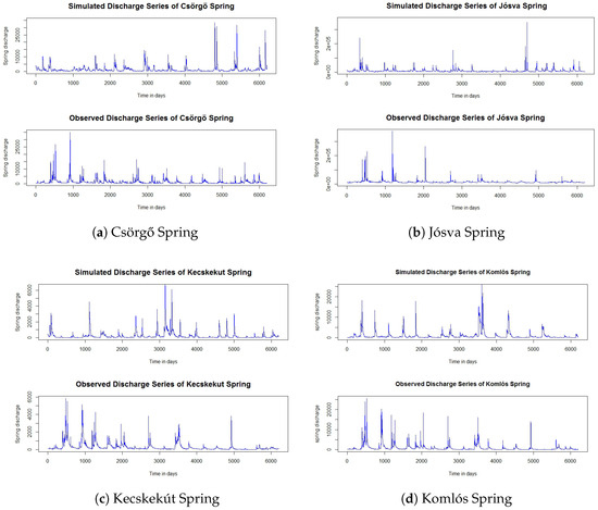
Figure 2.
Simulated and observed hydrographs (m3/day) of Csörgő, Jósva, Kecskekút, and Komlós Springs.
Although the ’eye test’ alone can be deceptive and misleading, plotting a classical ensemble mean or a ±SD ribbon is uninformative for a process driven by random time jumps; any goodness-of-fit measure based on point-by-point differences is inadequate. To illustrate, consider that in one year, the observed series might feature a flash flood on June 2, while the simulated series could exhibit a similar event on August 14. A difference-based metric would likely report a large mismatch, simply because one series contains an extreme event at a different time than the other. Since flash floods represent very large excursions from the base flow, they inevitably dominate such metrics—even though highlighting the exact time and extent of these excursions is not our objective and does not truly indicate overall fit. Among others reason, that is how the Nash–Sutcliffe Efficiency (NSE), a widely accepted performance metric in hydrology, suffers from exactly the same sensitivity to the timing and magnitude of individual peaks and is, therefore, unsuitable here.
Instead, we need a criterion that is insensitive to the timing of individual peaks. Therefore, we compare the quantiles of the simulated discharge process with those of the observed process. In this respect, Table 7 displays the mean ratio of simulated to observed discharge quantiles. The slight overestimation of these quantiles by the simulation, represented in the table by values greater than one, is consistent with a conservative stance: future flash floods may well exceed anything observed to date.
Table 7.
Mean ratio of simulated to observed discharge quantiles.
We do not attempt to match the entire distribution because
- 1.
- Stationarity of the process is unknown and not under investigation; and
- 2.
- Even if the process were stationary, the strong temporal dependence of daily discharges would bias distribution-wide estimates.
High-end values, however, are nearly independent under broad conditions, so high-quantile estimates are far more reliable than full-distribution estimates, providing the rationale of our method.
6.5. Scaling Check via Fractal Dimension
Because a distribution theory for fractal-dimension estimators is not yet available, constructing a formal hypothesis test is not feasible. To verify that the combined jump + fOUP model captures the multiscale roughness of the observed discharge time series, we perform a Monte-Carlo re-estimation exercise: 500 synthetic datasets are generated from the fitted model, and the fractal dimension is re-estimated on each run. The empirical spread (reported in Table 6) indicates that the point estimates are stable. While this is not a formal confidence interval, it provides a transparent indication of parameter uncertainty without invoking unverified asymptotics. We call it the empirical 90% confidence interval (CI), and the observed D values are evaluated against these intervals. Table 8 presents the observed D alongside the mean and dispersion of the simulated distribution, while Figure 3 visualizes the sampling distributions.
Table 8.
Fractal dimension (D) and implied Hurst exponent () for the observed and simulated discharge records.
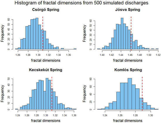
Figure 3.
Histogram of fractal-dimension estimates from 500 Monte-Carlo simulations for each spring. The vertical dashed red lines represent the observed D value.
For every spring, the observed D falls within the simulated 90% CI, consistently near its upper bound, indicating a slight positive bias, as also observable in Figure 3, but no statistically significant discrepancy. For example, at Csörgő Spring, the observed contrasts with a simulated mean of 1.291 (90% CI: 1.266–1.316).
Comparable agreement is obtained for Jósva, Kecskekút, and Komlós. This analysis confirms that the combined model faithfully reproduces the fractal roughness and the associated Hurst exponent () across scales.
The values in Table 8 describe the full jump + fOU process, so they are systematically lower (0.54–0.71) than the background in Table 5 (0.68–0.91); this confirms the well-known “spurious roughness” effect of jumps [36]: high-frequency jump spikes shorten the effective memory, whereas the jump-filtered baseline retains the longer-range dependence quantified in the Section 6.1. Simulation studies in the literature show that the madogram remains unbiased, but its variance increases when large jumps contaminate the signal [37]. In contrast, once jumps are removed, the fOUp-specific estimator regains full efficiency.
6.6. Validation on Accumulated Discharge
From a water resource management perspective, cumulative discharge is of paramount importance, as it directly reflects the volume of water available for various uses over a given period. Therefore, its accurate estimation is a key objective in hydrological modeling. Figure 4 demonstrates the performance of our model in this regard.
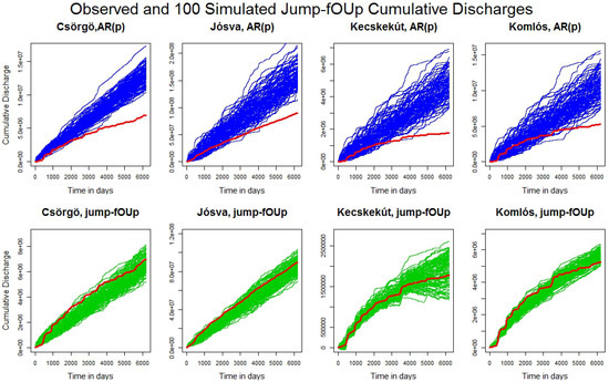
Figure 4.
Accumulated discharge comparison (m3/day): observed (red line) vs. jump–fOUp model (100 simulations, green lines) and jump–AR Model (100 simulations, blue lines) for Csörgő, Jósva, Kecskekút, and Komlós Springs.
To highlight the critical role of long-range dependence, we replace the background flow component with an autoregressive (AR) process while retaining the same jump sequence used in the jump–fOUp simulation. The outcome is striking: the 100 cumulative discharge trajectories generated by the AR model (blue lines) significantly overshoot the observed discharge (red line)—in some cases, more than doubling it by the end of the period. In contrast, simulations based on the fOUp model closely track the empirical data, underscoring the model’s accuracy. Moreover, the variability among the jump–AR simulations is substantially higher than that of the jump–fOUp simulations, reflecting the latter’s smoother trajectories. These results illustrate that the jump–fOUp model yields more reliable cumulative discharge estimates, enhancing its utility for water resource planning and management.
7. Discussion
7.1. Modeling Rationale
Karst springs exhibit fractal or multifractal, scale-invariant flow patterns due to complex conduit and matrix interactions. The fractal dimension (FD) measures this roughness and, as shown in our earlier paper [10], can be interpreted as the measure of the aquifer’s complexity; hence, it must be matched by any realistic model. In our approach, a jump–fOUp model integrates the following two primary controls of karst discharge within a single stochastic framework: the long-range dependent background flow—itself comprising multiple hydrogeological components—captured via the fractional Ornstein–Uhlenbeck process and the heavy-tailed recharge surges modeled through a renewal–reward jump process with correlated, heavy-tailed interarrival times and magnitudes. The fractional Ornstein–Uhlenbeck component encodes long-range dependence, ensuring that simulated series exhibit non-trivial FD. The interaction of the jump and the fractional Brownian motion component in the driving force of the fOUp dynamics finally reproduces the observed fractal dimension, which is different of the fBm’s FD. As noted in the Abstract, omitting fractal scaling (using short-memory noise) causes the accumulated discharge to exceed the realistic value substantially.
7.2. Model Goodness
Figure 2 illustrates that simulated and observed hydrographs exhibit strong visual agreement, while Table 8 confirms that the model replicates the observed fractal dimension within the limits of sampling error. This demonstrates that the jump–fOUp model provides a generative mechanism capable of faithfully reproducing these key features.
In comparison to short-memory AR baselines [5], the jump–fOUp model offers significantly improved tracking of cumulative discharge volumes (Figure 4). This highlights that omitting long-range dependence—governed by the Hurst parameter (H)—can lead to potentially flawed assessments of water resources. When the background flow, represented by the truncated process, is instead modeled with a short-memory AR(1) process, a single AR parameter must account for all temporal dependencies. This results in systematically higher AR parameter estimates compared to the memory parameter in the fOUp model. Moreover, because this parameter acts not only on the driving noise but also on the jumps, it dampens the jump effects more slowly than in the fOUp case, thereby forecasting elevated discharges in the following days. The cumulative result—total discharged water volume—becomes unrealistically high, yielding an overly optimistic outlook for water resource management.
7.3. Cross-Model Comparison
We do not include comparisons with further models like ARFIMA or Lévy-fOUp here. The discrete-time ARFIMA() process can be viewed as the discrete analog of the continuous-time fractional Ornstein–Uhlenbeck diffusion [38,39,40]. Because fOUp sample paths are almost surely continuous, they cannot, on their own, represent jumps. This limitation carries over to the ARFIMA discrete counterpart: the p-th-order AR term corresponds to the differential equation description, and the additional q-th-order MA term merely governs (increases) path smoothness and cannot introduce sharp discontinuities. Capturing jumps may require a Lévy-driven extension (Lévy–fOU) [41], however that approach is unable to represent the interdependence between the surges and the interarrival times. As our framework handles these mentioned phenomena provably well, any comparison with the above models would inevitably fail in those respects; hence, we do not conduct a full comparative analysis here.
7.4. Model Merits
The improved accuracy in cumulative discharge estimation provided by our model arises from two key components:
- (i)
- a fractional kernel that propagates hydrological memory across months to years; and
- (ii)
- Weibull–Weibull jump pairs, whose negative correlation between size and waiting time reflects the natural depletion–recharge dynamics of the aquifer (Table 3).
Unlike Poisson jump diffusions [42] or Lévy flights, the semi-Markov specification preserves both the heavy tail and the empirically observed dependence between surge size and lead time, a combination that classical multifractal surrogates describe but cannot generate mechanistically.
7.5. Possible Future Research Directions
Parameter identification remains demanding, and further research (e.g., investigating iterative, likelihood-based, or Bayesian approaches for discretely observed jump-fOU processes) would be beneficial. However, the current method yields parameters that produce simulations consistent with key empirical observations, including the crucial fractal dimension. Finally, extensions like time-varying or precipitation-driven jump intensities offer an avenue to embed climate signals directly into the discharge generator.
While the current framework is already deployable for spring-flow forecasting, several promising future applications remain to be explored: (i) extending long-term projections under climate-change scenarios by tailoring the jump and interarrival distributions; (ii) embedding the model in water resource management tools to quantify drought risk; and (iii) applying the approach to other intermittently driven time series, such as renewable generation spikes or high-frequency trading volumes. Before pursuing these extensions, it is important to conduct rigorous model-to-model comparisons to validate the new framework against existing approaches. In addition, a systematic assessment of the model’s sensitivity to parameter perturbations should be carried out to ensure that its behavior remains stable under parameter uncertainty. A comprehensive study could adopt the Morris method for preliminary screening [34], followed by Sobol indices for the most influential subset of parameters. Bai et al. [35] show that incorporating a fractal-dimension objective in calibration improves peak-flow realism, supporting the view that D (and, hence, H) is an important driver of flood peaks. Such analyses will help refine the practical interpretation of the estimated parameters, ensuring that each parameter’s role is well understood and grounded in physical significance. Together, these steps will provide greater confidence in the model’s reliability and guide the effective application of the framework to real-world scenarios.
8. Conclusions
The jump–fOUp model with a semi-Markov Weibull–Weibull jump structure effectively replicates the observed behavior of karst spring discharge series. It captures the empirical amplitude distributions of flow, the total cumulative discharge volumes, and the fractal dimensions of the time series for all four Hungarian springs studied herein. Long-range dependence (H > 0.5) in the fractional Ornstein–Uhlenbeck kernel is indispensable: replacing the fractional kernel with a short-memory noise leads to a substantial overestimation of total discharge (inflated by up to 50%).
Furthermore, the model accounts for the observed negative correlation between surge magnitude and interarrival time by modeling these variables jointly. This coupling of jump size and waiting time is crucial in reproducing realistic flood peaks in the simulations. Overall, the proposed framework concentrates on the fractal characterization by the fractal dimension of discharge variability and builds a stochastic differential-based process model. It may be extended by incorporating time-varying parameters or rainfall covariates to enhance predictive modeling of karst spring discharge dynamics.
Author Contributions
Conceptualization, L.M. and J.K.; Methodology, L.M., D.B. and E.B.; Software, D.B.; Validation, D.B., E.B. and A.D.; Formal Analysis, D.B. and L.M.; Investigation, E.B. and A.D.; Resources, J.K.; Data Curation, E.B. and J.K.; Writing—Original Draft Preparation, D.B. and L.M.; Writing—Review and Editing, L.M., J.K., D.B., E.B. and A.D.; Visualization, D.B. and L.M.; Supervision, L.M.; Project Administration, L.M. All authors have read and agreed to the published version of the manuscript.
Funding
This research received funding from the National Research, Development and Innovation Office within the framework of the Thematic Excellence Program 2021—National Research Sub programme: “Artificial intelligence, Large Networks, data security: mathematical foundation and applications” and the Artificial Intelligence National Laboratory Program (MILAB). The Ministry of Innovation and Technology of Hungary also provided support within the framework of the National Research, Development and Innovation Fund, which took part in financing this research under the Eötvös Loránd University TKP 2021-NKTA-62 funding scheme.
Data Availability Statement
The daily discharge data for the Aggtelek karst springs used in this study were originally collected by the Hungarian Water Resources Research Plc. (VITUKI) and are described in [28]. The processed data used for the analysis are available from the corresponding author upon reasonable request.
Acknowledgments
We thank the three anonymous referees for their insightful comments and constructive suggestions, improving significantly the readability and overall quality of the manuscript.
Conflicts of Interest
The authors declare no conflicts of interest. The funders had no role in the design of the study; in the collection, analyses, or interpretation of data; in the writing of the manuscript; or in the decision to publish the results.
Abbreviations
| AIC | Akaike Information Criterion |
| AR | Autoregressive |
| ARMA | Autoregressive Moving Average |
| CDF | Cumulative Distribution Function |
| ET | Energy Type (statistic) |
| fBm | Fractional Brownian motion |
| fGn | Fractional Gaussian noise |
| FD | Fractal Dimension |
| fOU | Fractional Ornstein–Uhlenbeck |
| fOUp | Fractional Ornstein–Uhlenbeck process |
| jump–fOUp | Jump Fractional Ornstein–Uhlenbeck process |
| K–S | Kolmogorov–Smirnov |
| LSE | Least Squares Estimator |
| MLE | Maximum Likelihood Estimation |
| OUp | Ornstein–Uhlenbeck process |
| Probability Density Function | |
| SD | Second Difference |
| SDE | Stochastic Differential Equation |
| VITUKI | Vízgazdálkodási Tudományos Kutató Intézet (Water Resource Research Institute) |
Appendix A. Proof of Theorem 1
Appendix A.1. Problem Setup
We are given a stochastic process () defined in (5) as follows:
Here, is a fractional Brownian motion (fBm) with a Hurst parameter (); is a càdlàg, non-decreasing renewal–reward process(implying J has only finitely many jumps on any compact time interval ); and is the initial condition, independent of and J. The constants (, , ) are given.
The integrals in (5) are understood as follows:
The term is a pathwise stochastic integral with respect to fBm.
- If , has sample paths that are almost surely Hölder continuous of any order (). Since can be chosen such that and the kernel () is Lipschitz continuous (hence, of bounded 1 variation) on , the integral exists pathwise as a Young integral [43]. The condition for existence is , where p is the variation exponent of the kernel and q is the variation exponent of the integrator. Here, (bounded variation) and has finite q variation for any . So, requires , which is always true. Thus, the Young integral exists.
- If , the paths of are rougher (infinite q variation for ). Although the standard Young theory might not directly apply based solely on Hölder exponents, the integral is still well defined pathwise using extended frameworks like fractional calculus integration developed by Zähle [44]. This approach defines when f possesses a certain fractional smoothness related to the roughness of g. Since our kernel () is in s, the necessary conditions are met for all .
We denote this integral simply by , understanding its pathwise nature (consistent with frameworks like Rough Paths [45]).
The term is a Riemann–Stieltjes integral. Since is a renewal–reward process, its sample paths are càdlàg, non-decreasing, and piecewise constant (step functions). Consequently, has almost surely bounded variation on any compact interval . The kernel () is continuous on . Therefore, the classical Riemann–Stieltjes integral exists pathwise for each realization (). It can be explicitly written as a finite sum over the jump times () of J:
where is the jump size () at time .
Our objective is to rigorously prove, using pathwise differentiation techniques, that , as defined by (5), satisfies the stochastic differential equation (SDE):
The term should be interpreted in the context of the pathwise integral theory, and represents the increments of the jump process.
The arguments above establish that both stochastic integrals in the definition (5) of are well defined pathwise for almost every realization () for all . The integral relies on the Young/Zähle theory, while uses the classical Riemann–Stieltjes theory for integrators of finite variation.
Appendix A.2. Differentiating the Terms of
We differentiate with respect to t by considering each term in (5). We employ appropriate Leibniz rules for pathwise Stieltjes integrals. Let , where , , and are the deterministic, fractional, and jump parts, respectively.
Appendix A.2.1. Deterministic Terms
The first two terms () are deterministic and smooth. Therefore,
Appendix A.2.2. Fractional Brownian Motion Term
Let . We need to compute . Since the integral is pathwise (Young/Zähle), we can apply a suitable Leibniz rule. For an integral (, where k is sufficiently smooth in t and the integral exists pathwise), the rule is formally expressed as follows:
This rule is rigorously justified in the context of Young integration [43] and its extensions [44,45] when .
We apply the rule to . Here, . Thus, and . We have the following:
Multiplying by , we arrive at the following:
Appendix A.2.3. Jump Term
Let . Since is a step function with bounded variation and is smooth, we can apply the Leibniz rule (A2) for Stieltjes integrals with replacing . Using and again yields the following:
Here, represents the Stieltjes differential of J. If t is not a jump time, . If is a jump time, corresponds to a measure with a mass of at . This formula correctly captures both the continuous evolution between jumps (where only the term is active) and the discrete jumps (where is active and equals ).
Appendix A.3. Combining the Differentials
Now, we sum the differentials of all parts of :
Substituting from (A1), (A3), and (A4) yields the following:
We simplify the coefficient of the term by using (5) rearranged as follows:
We substitute this into the coefficient:
Thus, the combined differential is expressed as follows:
This is precisely the target SDE (6).
In summary, we have rigorously shown that the process () defined by (5) satisfies the stochastic differential equation (6). The derivation relies on the pathwise interpretation of the stochastic integrals and standard rules of calculus applied to the deterministic part, combined with the Leibniz rule for pathwise Stieltjes integrals for the fractional and jump components. The calculation confirms that is the unique strong solution to the SDE (6).
Appendix B. Methodological Outline and Algorithm Pseudocode
To assist practitioners, we have prepared a summary table of recommended parameter defaults, model settings, and diagnostic checks. This table compiles the key findings of our study and the literature into a concise reference. Table A1 lists each parameter or setting, its typical value or how to choose it, and the main diagnostic to verify a good fit. Where appropriate, we cite the manuscript or other sources:
Table A1.
Summary of recommended defaults and diagnostic checks.
Table A1.
Summary of recommended defaults and diagnostic checks.
| Parameter/Setting | Recommended Default or Typical Value | Diagnostic/Notes |
|---|---|---|
| Mean reversion rate () | Very low (∼0.05–0.10 day−1) | Verify slow decay: check baseline auto-correlation |
| OU volatility () | Order – (see Table 4) | Match baseline variance (second differences) |
| Hurst exponent (H) | via madogram; typically 0.6–0.9 | Check fractal dimension: (Table 5) |
| Jump size (Weibull) | Fit Weibull, shape | KS test; inspect heavy tail |
| Jump timing (Weibull) | Shape –0.6, scale 10–20 | KS test; sub-exponential interarrival tail |
| Size–time correlation () | Negative (≈−0.2 … ) | Check empirical ; Gaussian copula in sim. |
| Jump detection threshold () | 97.5% quantile of | Sensitivity: vary 0.95–0.99 and refit |
| Baseline truncation threshold () | 90 % quantile of X | Ensure only spikes removed |
| Simulations (ensemble size) | ≥100 replicates | Ensemble mean ± SD should bracket data (Figure 3) |
| Diagnostics | Fractal dimension, cumulative discharge | e.g., on D by simulation |
| Algorithm A1 Simulation of Karst Spring Discharge using Jump-Diffusion fOU Model |
|
References
- Fiorillo, F. The Recession of Spring Hydrographs, Focused on Karst Aquifers. Water Resour. Manag. 2014, 28, 1781–1805. [Google Scholar] [CrossRef]
- Majone, B.; Bellin, A.; Borsato, A. Runoff generation in karst catchments: Multifractal analysis. J. Hydrol. 2004, 294, 176–195. [Google Scholar] [CrossRef]
- Goldscheider, N.; Mádl-Szőnyi, J.; Erőss, A.; Schill, E. Thermal water resources in carbonate rock aquifers. Hydrogeol. J. 2010, 18, 1303–1318. [Google Scholar] [CrossRef]
- Labat, D.; Hoang, C.T.; Masbou, J.; Mangin, A.; Tchiguirinskaia, I.; Lovejoy, S.; Schertzer, D. Multifractal behaviour of long-term karstic discharge fluctuations. Hydrol. Process. 2012, 26, 1072–1083. [Google Scholar] [CrossRef]
- Labat, D.; Mangin, A.; Ababou, R. Rainfall–runoff relations for karstic springs: Multifractal analyses. J. Hydrol. 2002, 256, 176–195. [Google Scholar] [CrossRef]
- Pardo-Igúzquiza, E.; Dowd, P.A.; Durán, J.J.; Robledo-Ardila, P. A review of fractals in karst. Int. J. Speleol. 2019, 48, 11–20. [Google Scholar] [CrossRef]
- Mandelbrot, B.B. Fractals: Form, Chance, and Dimension, Revised ed.; W. H. Freeman: San Francisco, CA, USA, 1977. [Google Scholar]
- Addison, P. Fractals and Chaos: An Illustrated Course; Institute of Physics Publishing: Bristol, UK, 1997. [Google Scholar] [CrossRef]
- Hergarten, S.; Birk, S. A fractal approach to the recession of spring hydrographs. Geophys. Res. Lett. 2007, 34, L11401. [Google Scholar] [CrossRef]
- Borbás, E.; Márkus, L.; Darougi, A.; Kovács, J. Characterization of karstic aquifer complexity using fractal dimensions. GEM—Int. J. Geomathematics 2021, 12, 4. [Google Scholar] [CrossRef]
- Schertzer, D.; Lovejoy, S. Multifractals, generalized scale invariance and complexity in geophysics. Int. J. Bifurcat. Chaos 2011, 21, 3417–3456. [Google Scholar] [CrossRef]
- Biagini, F.; Hu, Y.; Øksendal, B.; Zhang, T. Stochastic Calculus for Fractional Brownian Motion and Applications; Springer: London, UK, 2008. [Google Scholar] [CrossRef]
- Ross, S.M. Stochastic Processes, 2nd ed.; John Wiley & Sons: New York, NY, USA, 1996. [Google Scholar]
- Sugiyama, H.; Vudhivanich, A.C.; Lorsirirat, W.K. Stochastic flow duration curves for evaluation of flow regimes in rivers. J. Am. Water Resour. Assoc. 2003, 39, 47–58. [Google Scholar] [CrossRef]
- Leone, G.; Pagnozzi, M.; Catani, V.; Ventafridda, G.; Esposito, L.; Fiorillo, F. A hundred years of Caposele spring discharge measurements: Trends and statistics for understanding water resource availability under climate change. Stoch. Environ. Res. Risk Assess. 2020, 34, 123–148. [Google Scholar] [CrossRef]
- Kleptsina, M.L.; Le Breton, A. Statistical analysis of the fractional Ornstein–Uhlenbeck type process. Stat. Inference Stoch. Process. 2002, 5, 229–248. [Google Scholar] [CrossRef]
- Bercu, B.; Courtin, S.; Savy, N. MLE for the drift parameter of the fractional Ornstein–Uhlenbeck process. arXiv 2016, arXiv:1604.04030. [Google Scholar]
- Tanaka, K.; Xiao, W.; Yu, J. Maximum likelihood estimation for the fractional Ornstein–Uhlenbeck process with discrete observations. Econom. Theory 2020, 36, 929–962. [Google Scholar]
- Lohvinenko, T.; Ralchenko, K. Parameter estimation for the fractional Ornstein–Uhlenbeck process with periodic mean. Mod. Stoch. Theory Appl. 2019, 6, 337–355. [Google Scholar]
- Hu, Y.; Nualart, D. Parameter estimation for fractional Ornstein–Uhlenbeck processes. Stat. Probab. Lett. 2010, 80, 1030–1038. [Google Scholar] [CrossRef]
- Hu, Y.; Nualart, D.; Zhou, H. Parameter estimation for fractional Ornstein–Uhlenbeck processes of general Hurst parameter. Stat. Inference Stoch. Process. 2017, 22, 111–142. [Google Scholar] [CrossRef]
- Xiao, W.; Wang, X.; Yu, J. Estimation and Inference in Fractional Ornstein–Uhlenbeck Model with Discrete-Sampled Data. Unpublished Manuscript. 2018. Available online: https://www.stern.nyu.edu/sites/default/files/assets/documents/TwostagefVm09.pdf (accessed on 10 October 2024).
- Telbisz, T.; Gruber, P.; Mari, L.; Kőszeghi, M.; Bottlik, Z.; Standovár, T. Geological heritage, geotourism and local development in Aggtelek National Park (NE Hungary). Geoheritage 2020, 12, 5. [Google Scholar] [CrossRef]
- Hevesi, A. Magyarország karsztvidékeinek kialakulása és formakincse I–II. Földr. Közl. 1991, 115, 25–35, 99–120. (In Hungarian) [Google Scholar]
- Haas, J. Geology of Hungary; Springer: Berlin/Heidelberg, Germany, 2012. [Google Scholar] [CrossRef]
- Grill, J.; Kovács, S.; Less, G.; Réti, Z.; Róth, L.; Szentpétery, I. Az Aggtelek–Rudabányai-hegység főtektonikai felépítése és fejlődéstörténete. Földt. Kut. 1984, 27, 49–56. (In Hungarian) [Google Scholar]
- Less, G. Polyphase evolution of the structure of the Aggtelek–Rudabánya Mountains (NE Hungary), the southern element of the inner Western Carpathians—A review. Slovak Geol. Mag. 2000, 6, 260–268. [Google Scholar]
- Maucha, L. Az Aggtelek-Hegység Karszthidrológiai kutatáSai Eredményei és Zavartalan Hidrológiai Adatsorai 1958–1993; VITUKI Rt., Hydrological Institute: Budapest, Hungary, 1998. (In Hungarian) [Google Scholar]
- Kordos, L. Magyarország Barlangjai; Gondolat Kiadó: Budapest, Hungary, 1984. (In Hungarian) [Google Scholar]
- Székely, K. (Ed.) Magyarország Fokozottan véDett Barlangjai; Mezőgazda Kiadó: Budapest, Hungary, 2003. (In Hungarian) [Google Scholar]
- Kloeden, P.E.; Zhang, T. Numerical Methods for Fractional Stochastic Differential Equations; Springer: Berlin/Heidelberg, Germany, 2024. [Google Scholar]
- Kalantan, Z.I.; Abd Elaal, M.K. A new family based on lifetime distribution: Bivariate Weibull–G models based on Gaussian copula. Int. J. Adv. Appl. Sci. 2018, 5, 100–111. [Google Scholar] [CrossRef]
- Ahmed, M.; Ali, A.; Kharaz, A. Local dependence for bivariate Weibull distributions created by Archimedean copula. Math. Stat. Appl. 2021, 18, 38. [Google Scholar]
- Morris, M.D. Factorial sampling plans for preliminary computational experiments. Technometrics 1991, 33, 161–174. [Google Scholar] [CrossRef]
- Bai, Z.; Wu, Y.; Ma, D.; Xu, Y.-P. A new fractal-theory-based criterion for hydrological model calibration. Hydrol. Earth Syst. Sci. 2021, 25, 3675–3690. [Google Scholar] [CrossRef]
- Bardet, J.M.; Surgailis, D. Influence of discontinuities on Hurst-parameter estimation. Ann. Inst. H. Poincaré 2020, 56, 1757–1792. [Google Scholar]
- Gaume, L.; Lantuéjoul, C. Robustness of variogram and madogram estimators in the presence of outliers and jumps. Math. Geosci. 2019, 51, 245–268. [Google Scholar]
- Cheridito, P.; Kawaguchi, H.; Maejima, M. Fractional Ornstein–Uhlenbeck processes. Electron. J. Probab. 2003, 8, 1–14. [Google Scholar] [CrossRef]
- Granger, C.W.J.; Joyeux, R. An introduction to long-memory time-series models and fractional differencing. J. Time Ser. Anal. 1980, 1, 15–29. [Google Scholar] [CrossRef]
- Hosking, J.R.M. Fractional differencing. Biometrika 1981, 68, 165–176. [Google Scholar] [CrossRef]
- Wolpert, R.L.; Taqqu, M.S. Fractional Ornstein–Uhlenbeck Lévy processes and the Telecom process: Upstairs and downstairs. Signal Process. 2005, 85, 1523–1545. [Google Scholar] [CrossRef]
- Veneziano, D.; Essiam, A.K. Flow through porous media with multifractal hydraulic conductivity. Water Resour. Res. 2003, 39, 1291. [Google Scholar] [CrossRef]
- Young, L.C. An inequality of the Hölder type, connected with Stieltjes integration. Acta Math. 1936, 67, 251–282. [Google Scholar] [CrossRef]
- Zähle, M. Integration with respect to fractal functions and stochastic calculus I. Probab. Theory Relat. Fields 1998, 111, 333–374. [Google Scholar] [CrossRef]
- Friz, P.K.; Hairer, M. A Course on Rough Paths: With an Introduction to Regularity Structures; Springer: Cham, Switzerland, 2014. [Google Scholar] [CrossRef]
Disclaimer/Publisher’s Note: The statements, opinions and data contained in all publications are solely those of the individual author(s) and contributor(s) and not of MDPI and/or the editor(s). MDPI and/or the editor(s) disclaim responsibility for any injury to people or property resulting from any ideas, methods, instructions or products referred to in the content. |
© 2025 by the authors. Licensee MDPI, Basel, Switzerland. This article is an open access article distributed under the terms and conditions of the Creative Commons Attribution (CC BY) license (https://creativecommons.org/licenses/by/4.0/).