Abstract
This study proposes a four-module “decomposition–forecasting–ensemble–correction” framework to improve the accuracy of complex coal price forecasts. The framework combines Variational Mode Decomposition (VMD), adaptive Autoregressive Integrated Moving Average (ARIMA) and Gated Recurrent Unit (GRU)-Attention forecasting models, a data-driven weighted ensemble strategy, and an innovative error correction mechanism. Empirical analysis using the Bohai-Rim Steam–Coal Price Index (BSPI) shows that the framework significantly outperforms benchmark models, as validated by the Diebold–Mariano test. It reduces the Mean Absolute Percentage Error (MAPE) by 30.8% compared to a standalone GRU-Attention model, with the error correction module alone contributing a 25.1% MAPE reduction. This modular and transferable framework provides a promising approach for improving forecasting accuracy in complex and volatile economic time series.
Keywords:
coal price forecasting; variational mode decomposition; error self-correction; GRU-Attention; weight optimization MSC:
91B84; 68T07
1. Introduction
China, as the world’s largest producer and consumer of coal, accounts for over half of the global total in both categories. Coal plays a fundamental role in the Chinese economy, supporting nearly 60% of the nation’s power supply [1] and serving as the primary energy source for foundational industries such as steel, cement, and chemical manufacturing. Consequently, the stability of coal prices is crucial for macroeconomic stability, making their scientific forecasting a task of significant theoretical value and practical importance.
However, forecasting coal prices is a highly challenging task. Its price formation is complex, driven by a multitude of factors including macroeconomic cycles, industrial policy adjustments, supply–demand dynamics, and geopolitical events. As a result, the price series exhibits prominent non-linear, non-stationary, and time-varying characteristics. These complex features expose the limitations of existing forecasting methods: classical statistical models (such as ARIMA) rely on stationarity assumptions and struggle to capture non-linear price dynamics; traditional machine learning models, while possessing non-linear fitting capabilities, face difficulties in effectively handling temporal dependencies in sequences; deep learning models, despite breakthroughs in sequence modeling, still encounter performance bottlenecks and lack sufficient interpretability when processing such complex price series independently.
To address these difficulties, the decomposition–ensemble paradigm offers a new approach. This paradigm employs a “divide and conquer” strategy through its three core modules: it first decomposes a complex series into simpler modal components, then forecasts each component separately, and finally ensembles the individual forecasts into a unified result. A large body of research has demonstrated that this paradigm can significantly enhance the forecasting performance for complex time series.
Despite their success, existing decomposition–ensemble paradigms have two critical deficiencies. First, the traditional three-module architecture neglects error propagation and accumulation, lacking a global correction mechanism. Second, the paradigm’s flexibility, while offering a rich selection of components, complicates both component selection and parameter optimization.
To address these challenges, we propose an enhanced forecasting framework based on the decomposition–ensemble paradigm, with innovations at two levels:
Architecturally, we introduce a four-module “decomposition–forecasting–ensemble–correction” architecture that adds an independent correction module to the classic three-module structure. This new module is designed to identify and rectify accumulated systematic errors, thereby optimizing global forecasting performance.
Methodologically, guided by Occam’s razor, we avoid the blind stacking of complex models. Instead, we construct a high-performance system through the synergistic coordination and optimization of general-purpose models and mature algorithms. Specifically, we deploy parallel ARIMA and GRU models for each mode and use a data-driven linear weighting algorithm to achieve a concise yet robust forecast ensemble.
Our main contributions are threefold: (1) A novel four-module forecasting architecture with a global error correction capability to address error accumulation in traditional paradigms. (2) A concise and efficient strategy of synergistic component coordination that resolves the selection and optimization challenges posed by the paradigm’s flexibility. (3) A systematic empirical study that validates our framework’s superiority, providing an effective new tool for forecasting complex economic time series.
The remainder of this paper is organized as follows. Section 2 reviews the related literature. Section 3 details our proposed framework. Section 4 describes the experimental design, and Section 5 presents and discusses the results, including an ablation study. Finally, Section 6 concludes the paper and outlines future work.
2. Literature Review
The inherent complexity of price series has driven the continuous evolution of forecasting methodologies. This section systematically reviews this trajectory to provide the theoretical and technical foundations for the enhanced framework we propose.
2.1. Evolution of Single Forecasting Models
The evolution of single forecasting models reflects the field’s effort to address data complexity with better tools. Based on modeling principles and technical characteristics, this evolution can be divided into three stages:
Classical Statistical Model Stage. Early research in price forecasting predominantly employed classical time series models such as ARIMA and Vector Autoregression (VAR) [2]. ARIMA, with its clear statistical principles and mature parameter estimation methods, is commonly used as a benchmark for forecasting performance [3]. However, its linearity assumption and stationarity requirement limit its performance when processing modern price series with non-linear and non-stationary characteristics [4].
Machine Learning Model Stage. To address the limitations of linear models, machine learning approaches such as Support Vector Regression (SVR) and Artificial Neural Networks (ANN) have been applied to price forecasting. With their strong non-linear fitting capabilities, these models deliver higher accuracy when predicting non-linear economic time series [5]. Among them, SVR not only outperforms linear models but also offers greater robustness than complex deep learning models, particularly in scenarios involving small datasets or high-dimensional inputs [6]. However, as these models are inherently designed for static data, they face challenges in capturing the long-term dependencies characteristic of time series [7].
Deep Learning Model Stage. Recurrent Neural Networks (RNN) and their variants, such as Long Short-Term Memory (LSTM) and Gated Recurrent Unit (GRU), have revolutionized sequence modeling. Designed specifically for this purpose, these models leverage internal “memory” mechanisms to effectively capture temporal information, achieving notable improvements in forecasting accuracy over traditional machine learning approaches [8]. Among these, GRU, as a simplified variant of LSTM, has gained popularity due to its streamlined structure, fewer parameters, and high training efficiency [9]. More recently, the introduction of the Transformer architecture has pushed sequence modeling technology even further. With its self-attention mechanism, the Transformer demonstrates unique strengths in handling long sequences [10].
In parallel with deep learning advancements, other modern forecasting architectures designed to enhance robustness and automation have also gained attention. A notable example is Facebook’s Prophet [11], a component-based statistical model capable of handling seasonality, trend shifts, and holiday effects. Its proven effectiveness in complex commodity price forecasting highlights its value in addressing specific forecasting challenges [12].
Despite these advancements, all single models have inherent inductive biases that limit their ability to simultaneously handle the heterogeneous patterns (trends, cycles, perturbations) in complex price series [13]. Furthermore, the “black-box” nature of deep learning models restricts their interpretability and practical value [14].
2.2. Technical Development of the Decomposition–Ensemble Paradigm
To overcome these limitations, the “decomposition–ensemble” paradigm emerged, with technical developments focused on its three modules:
Decomposition Algorithms. Early research primarily used traditional methods such as Wavelet Transform (WT) and Empirical Mode Decomposition (EMD). However, WT lacks adaptability, while EMD suffers from the problem of mode mixing, both of which constrain decomposition quality [15]. VMD, with its solid foundation in variational theory, can effectively avoid mode mixing and achieve adaptive decomposition, gradually becoming the mainstream technology [16].
Differentiated Forecaster Configuration. While early approaches applied a uniform forecasting model to all decomposed components, modern research generally adopts differentiated configuration strategies, selecting appropriate models based on the statistical properties of each modal component [17]. For example, linear models such as ARIMA are applied to stable, low-frequency components, while more complex non-linear models are assigned to volatile, high-frequency ones. This includes classic machine learning models like SVR as well as deep learning models such as LSTM and GRU [18,19].
Ensemble Strategy Trade-offs: Most research favors linear ensemble methods (such as weighted averaging) for their simple structure, computational efficiency, and robustness against overfitting [20]. Some research also explores non-linear strategies, such as using neural networks or support vector machines as “meta-learners” for a more complex fusion of component forecasts [21]. However, these complex methods are prone to overfitting with limited sample sizes and incur significant computational costs [22].
2.3. Evolution of Approaches to Error Handling
The approach to handling the inevitable errors in forecasting has evolved from indirect optimization to explicit modeling, reflecting a deeper understanding of model uncertainty.
The traditional indirect approach treats forecasting errors as passive byproducts of model optimization. Under this view, errors serve only as a performance metric, and the only path to their reduction is to improve the forecasting model itself (e.g., by using better algorithms or optimizing hyperparameters).
In contrast, the modern explicit modeling approach transforms errors into modeling objects that contain useful information. This is based on the insight that errors often contain non-random patterns missed by the primary model, and modeling this residual information can further improve forecasting performance [23].
This explicit error modeling typically appears in two scenarios in time series forecasting:
The “Serial Correction” Pattern in Single-Model Forecasting. This method treats forecasting residuals as modellable objects, training a residual model to forecast the primary model’s errors, thereby correcting its output. This design philosophy of serial correction is highly consistent with two-stage regression in econometrics and the Boosting algorithm in machine learning [24]. Various serial forms of primary models and residual models have been developed in empirical research, such as “ARIMA-Neural Network”, “LSTM-SVR”, and “CNN-LSTM” [25,26,27].
The “Parallel Processing” Pattern in the Decomposition-Ensemble Framework. De-composition algorithms typically cannot completely decompose the original series, often leaving a residual in addition to the finite modal components. Parallel processing treats this residual as an additional modal component, forecasting it in parallel with the other modal components and then integrating it into the final result [28], thus fully utilizing the residual information.
2.4. Research Gap Identification and Study Positioning
A systematic literature review reveals two critical gaps in current price forecasting research:
First, existing decomposition–ensemble paradigms lack global error control. Their classic three-module architecture neglects error propagation and accumulation across stages, and current explicit error modeling techniques are applied only locally (e.g., at the decomposition stage or for single models), failing to achieve systematic control over the entire forecasting process.
Second, the flexibility of decomposition–ensemble paradigms often leads to a “complexity race” in practice, where researchers introduce increasingly novel and sophisticated components to improve performance. While this can enhance forecasting accuracy, it also dramatically increases system complexity, leading to higher computational costs, implementation difficulties, and a greater risk of overfitting.
Addressing these gaps, this study proposes an enhanced coal price forecasting framework that both solves the global error accumulation problem through a dedicated “correction” module and explores how to achieve high performance through the synergistic coordination of simpler, general-purpose models, rather than by escalating model complexity.
3. Methodology
3.1. Overall Design of the Enhanced Coal Price Forecasting Framework
Our enhanced coal price forecasting framework uses a four-module serial architecture: “decomposition–forecasting–ensemble–correction,” as illustrated in Figure 1. The functions of each module are as follows:
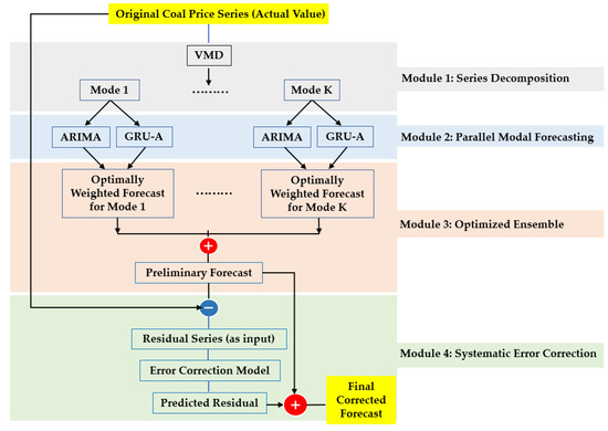
Figure 1.
Schematic of the enhanced forecasting framework.
- Module 1: Series Decomposition. The VMD algorithm decomposes the original coal price series into several modal components, each with distinct frequency characteristics. This lays the foundation for the subsequent forecasting stage.
- Module 2: Parallel Modal Forecasting. For each decomposed mode, an ARIMA and a GRU-Attention model are deployed in parallel, with the former capturing linear features and the latter mining non-linear dynamic patterns.
- Module 3: Optimized Ensemble. Using a data-driven, multi-scheme weight optimization strategy, the linear and non-linear forecasts for each mode are optimally ensembled. These modal forecasts are then aggregated to reconstruct a preliminary overall price forecast.
- Module 4: Systematic Error Correction. The systematic error accumulated from the preceding modules is treated as an independent modeling object. An error correction model is then trained to correct the preliminary forecast, yielding the final price forecast.
3.2. Series Decomposition: VMD-Based Implementation
We employ the VMD algorithm to decompose the original coal price series into K predetermined modal components, collectively denoted as the set . VMD achieves this by solving a constrained variational problem where each modal component, , is a compact band-limited signal centered around a frequency, , that is estimated concurrently.
where denotes the convolution operator, represents the partial derivative with respect to time t, and the expression is the analytic signal of derived via the Hilbert transform, which is used to determine the bandwidth of the signal.
VMD was selected as the core decomposition tool for two reasons. The primary reason is its technical effectiveness: it simplifies the forecasting task by decomposing the complex original series into simpler modal components.
A second, and crucial, advantage of VMD is its potential for economic interpretability. This potential arises because coal price fluctuations are themselves a composite of multi-scale economic factors—macroeconomic fundamentals determining long-term trends, seasonal factors influencing medium-term cycles, and sudden events causing short-term perturbations. Because VMD is effective at separating components by frequency, it allows each decomposed mode to be potentially correlated with a specific economic driver. This, in turn, endows the entire framework with a valuable degree of economic interpretability.
However, VMD’s performance is highly dependent on its parameters: the number of modes, K, and the penalty factor, α. Improper settings can lead to mode mixing or over-decomposition. Therefore, optimizing K and α is a critical step (detailed in Section 4.3.1).
3.3. Parallel Modal Forecasting: A Synergistic Adaptive Dual-Model Design
Given that VMD modal components exhibit both linear and non-linear dynamics, we construct a dual-model parallel forecasting architecture and introduce a synergistic adaptive mechanism. This mechanism enables the two heterogeneous models to respond to real-time data changes during the forecasting process and to transition from static to adaptive dynamic forecasting.
3.3.1. Linear Forecasting Unit: Dynamic ARIMA
For each modal component, we construct an ARIMA (p, d, q) model. Its orders are determined on the training set using the Box-Jenkins methodology.
To enhance performance, we implement a critical dynamic adaptation for the ARIMA model by employing a “fixed orders, re-estimated coefficients” strategy during the forecasting phase. This practice is also recommended by mainstream Python libraries such as statsmodels. This means that while the model’s orders (p, d, q) are held constant, its AR and MA coefficients are dynamically re-estimated as new data becomes available.
This optimized design allows the ARIMA unit to keenly respond to the latest data changes without sacrificing structural stability. This, in turn, significantly enhances the model’s adaptive capability during the forecasting phase.
3.3.2. Non-Linear Forecasting Unit: GRU with Attention Mechanism
We employ a GRU network to capture complex non-linear patterns in the modal components, as its unique gate mechanisms are highly effective for learning long-term dependencies.
However, a standard GRU’s parameters are fixed after training. Consequently, during the forecasting phase, it processes all inputs statically, lacking the ability to dynamically adapt to new data. This creates a distinct “adaptivity imbalance” when contrasted with our dynamic ARIMA model, which can re-estimate its coefficients. To resolve this, we integrate an attention mechanism after the GRU layer [29], endowing the unit with comparable dynamic adaptability.
The workflow is as follows: for each forecast, the GRU-Attention unit extracts a historical look-back window of length L, denoted as . This sequence is fed into the GRU layer, generating a corresponding sequence of hidden states, , which the attention mechanism uses to generate attention weights. Unlike a neural network’s parameters which remain fixed after training, these attention weights are calculated dynamically for each forecast based on the specific input.
We adopt the multiplicative attention mechanism proposed by Luong et al. [30], which involves these steps:
- Calculate Compatibility Scores: The final hidden state, , is compared with all preceding states () in the look-back window to assess their relevance to the current forecast, yielding compatibility scores.
- Generate Attention Weights: The softmax function normalizes these scores to produce attention weights, , where each weight quantifies the attention placed on the i-th historical time step.
- Construct the Context Vector: A dynamic context vector, , is formed as a weighted sum of the hidden states. This vector, summarizing the most relevant historical information, is then passed through a fully connected layer to yield the final modal forecast.
This design gives the GRU a dynamic adaptability comparable to the ARIMA’s coefficient re-estimation, allowing it to adapt by adjusting its focus on historical information without altering core network parameters.
3.3.3. Synergistic Adaptive Design
This module’s core innovation is its synergistic adaptive design, ensuring both parallel linear and non-linear units keenly respond to new data. This adaptivity is achieved at two different levels:
- The Dynamic ARIMA Unit performs coefficient-level adaptation, dynamically adjusting model coefficients for each forecast via the “fixed orders, re-estimated coefficients” strategy.
- The GRU-Attention Unit performs information-processing-level adaptation, recalculating attention weights on historical data in real-time for each forecast.
This synergistic design gives the dual-model module real-time adaptability, building upon the complementary strengths of its linear and non-linear components. Faced with new data, the module can perceive the latest trends while intelligently reviewing key historical information, significantly enhancing its forecasting performance and robustness on complex, time-varying data.
3.4. Optimized Ensemble: A Multi-Scheme Weight Optimization Strategy
This module is responsible for ensembling the parallel forecasts into a single, unified forecast value, and the ensemble process encompasses two stages: intra-modal ensemble and cross-modal reconstruction. Due to the relatively limited sample size of this study (N = 588) and the overfitting risk posed by complex non-linear ensemble algorithms (such as meta-learners), we adopt a robust linear weighted ensemble method.
3.4.1. Intra-Modal Ensemble: Weight Optimization Based on Multi-Scheme Evaluation
For mode k, its ensembled forecast value, , is obtained by the weighted summation of the ARIMA forecast, , and the GRU-Attention forecast, :
Weight determination constitutes the core of this step. The traditional inverse-error method typically relies on the selection of a single error metric, such as Root Mean Square Error (RMSE) or Mean Absolute Error (MAE), which may introduce subjectivity in metric selection [31]. Therefore, we design a data-driven weight optimization strategy to tailor the optimal ensemble weights for each mode:
Step 1: Generation of Candidate Weight Schemes
The RMSE, MAE, and MAPE for the ARIMA and GRU-Attention models are calculated on the training set, and three candidate weight schemes are generated using the inverse-error method. For example, the weights based on RMSE are calculated as follows:
where (for the ARIMA model) and (for the GRU-Attention model) are the root mean square errors for mode k on the training set. Similarly, the other two sets of candidate weights based on MAE and MAPE can be calculated.
Step 2: Optimal Scheme Selection
The three candidate weights are substituted into Equation (2) to generate corresponding in-sample forecast series on the training set. The MAPE value of each forecast series is then calculated, and the weight scheme that minimizes MAPE is selected as the final ensemble weights for mode k.
3.4.2. Cross-Modal Reconstruction
According to the additive constraint principle of VMD (i.e., the original series is approximately equal to the sum of all modal components), the ensembled forecasts for each mode, , are directly summed to reconstruct the preliminary overall forecast :
where K is the total number of modes from the VMD.
3.5. Systematic Error Correction: Explicit Error Modeling
Systematic error correction is the core innovation of our enhanced forecasting framework. It is designed to explicitly model and compensate for the cumulative error generated in the preceding stages, thereby further enhancing overall forecasting performance.
3.5.1. Error Accumulation and the Necessity for Correction
In the aforementioned decomposition–forecasting–ensemble modules, errors are generated endogenously and accumulate across stages. Based on their generation mechanisms and sources, these errors can be categorized into the following four types:
- Decomposition Error: As an approximation algorithm, VMD incurs information loss during the decomposition of the original series, resulting in a structural decomposition residual.
- Forecasting Error: The forecasting models for each mode are essentially function approximations of the true dynamics; they cannot perfectly capture all variation patterns, thus inevitably introducing forecasting biases.
- Intra-modal Ensemble Error: The linear weighted ensemble is a simplified treatment of the relationship between the two heterogeneous models and cannot fully capture their potential non-linear complementary effects.
- Cross-modal Ensemble Error: Direct summation for reconstruction overlooks the complex coupling relationships that may exist among different frequency components in the real economic system.
Collectively, these four types of errors constitute a systematic deviation between the preliminary overall forecast, , and the actual value, . We define this deviation as the overall forecasting residual series, :
This residual series contains non-random information that the primary forecasting model failed to capture. Modeling this residual series is therefore critical for compensating for the framework’s inherent deficiencies.
3.5.2. Residual Modeling Based on GRU-Attention
We use the same GRU-Attention architecture used for modal forecasting to construct an independent error correction model. This model takes the historical residual series, , as input, learns the dynamic patterns contained within, and generates the residual forecast for the next time step, .
Adding the forecasted residual value to the preliminary overall forecast from Section 3.4.2 produces the final corrected forecast:
By introducing the error correction module, we successfully extend the classic “serial correction” concept to the complex decomposition–ensemble architecture, constructing a corrective feedback loop that proceeds from “preliminary forecast” to “residual evaluation” and then to “secondary correction.” This design theoretically addresses the systematic deficiencies of the classic three-module architecture and enhances the accuracy and reliability of the forecasts.
3.6. Hyperparameter Optimization Strategy: Optuna Framework
The performance of deep learning models like GRU-Attention is highly dependent on their hyperparameter configuration. We use Optuna, an advanced automated hyperparameter optimization framework [32], to efficiently and systematically optimize these hyperparameters.
Optuna offers two key advantages for this study. First, its Bayesian optimization algorithm (based on the Tree-structured Parzen Estimator, or TPE) intelligently uses historical trial results to guide its search. Compared to grid search or traditional metaheuristics (such as genetic algorithms or particle swarm optimization), TPE finds optimal solutions with fewer trials when handling computationally expensive deep learning tasks [33]. Second, its intelligent pruning mechanism monitors trials in real-time and terminates poor performers early based on preset objectives [34]. This concentrates computational resources on the most promising hyperparameter combinations, significantly enhancing overall optimization efficiency.
We therefore use Optuna to optimize the GRU-Attention model’s key hyperparameters. The specific configurations for the Optuna search, including search spaces and trial counts, are detailed in Section 4.4.2.
3.7. Model Evaluation Metrics
We evaluate forecasting performance using three classic error metrics: MAPE, RMSE, and MAE. To strengthen the comparative analysis, we include two supplementary metrics: Theil’s U statistic and Directional Accuracy (DA). We also employ the Diebold–Mariano test (DM test) to assess statistical significance.
- MAPE measures relative error as a percentage, making it suitable for cross-scale comparisons. RMSE, due to its squared term, is highly sensitive to large errors and effectively highlights extreme deviations. MAE represents the average magnitude of absolute errors, providing straightforward interpretability. For all three metrics, smaller values indicate better forecasting accuracy. The formulas are:where is the actual value, is the forecasted value, and N is the total number of samples in the test set.
- Theil’s U Statistic: Compares the model’s accuracy to a naive “random walk” forecast, where the next value equals the current value. A value below 1 indicates the model outperforms the naive benchmark, while a value above 1 suggests inferior performance.
- DA: Assesses the model’s ability to predict the direction of changes (e.g., increase or decrease). This metric is particularly important in economic forecasting, where the direction can be as critical as the magnitude. DA is expressed as the percentage of correct directional predictions.
- DM test: Evaluates whether the difference in predictive accuracy between two models is statistically significant. The null hypothesis () assumes both models have equal forecasting accuracy. A p-value below a chosen significance level (e.g., 0.05) indicates a statistically significant difference, supporting the superiority of one model.
3.8. Forecasting System Implementation and Workflow
Implementing the four-module framework described previously creates a complete forecasting system. Its workflow comprises two stages: initial model training and rolling forecast validation.
3.8.1. Stage One: Initial Model Training
This stage involves training and configuring all system components on the historical dataset. The steps are as follows:
- VMD Parameter Optimization and Decomposition: After determining the optimal VMD parameters (K and α) on the training set, the set is decomposed into K modal components.
- Modal Forecaster Training: For each mode, an ARIMA and a GRU-Attention model are trained.
- Ensemble Weight Determination: The multi-scheme optimization strategy is applied to determine the optimal ensemble weights for each mode.
- Residual Series Generation: A preliminary forecast is generated on the training set using the trained models and weights, from which the residual series is calculated.
- Error Correction Model Training: An independent GRU-Attention model is trained on the generated residual series to serve as the error corrector.
3.8.2. Stage Two: Rolling Forecast Validation
To simulate a real-world environment, we evaluate the model on the test set via a one-step rolling forecast mechanism, as illustrated in Figure 2.
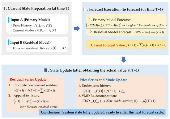
Figure 2.
The rolling forecast loop (T → T + 1).
This loop continuously iterates between forecasting and updating. At any time step T, the system integrates the primary and error correction models to generate the forecast When the actual price is revealed, the system immediately updates by: (1) updating the internal residual series with the new forecast error, and (2) incorporating the new price into the historical data and re-running the VMD to prepare for the next forecast.
A crucial design decision is the use of dynamic VMD re-decomposition with fixed parameters.
Dynamic re-decomposition ensures the modes capture the latest market dynamics. We reject the common practice of a one-time, upfront decomposition of the entire dataset, as it causes severe data leakage and is inapplicable in practice [35,36]. Instead, we regenerate the modes at each forecasting step using all currently available data [37]. While this increases computational cost, it is a necessary trade-off to ensure the model’s timeliness and the fairness of the evaluation.
However, dynamic re-decomposition can cause mode drift, where significant statistical differences between new and old modes lead to model failure. To mitigate this, we consistently use the same optimal VMD parameters (K and α) determined during the initial training. These fixed parameters act as a constant benchmark, imposing a uniform constraint on each decomposition. This maximizes modal consistency in terms of physical meaning and statistical properties, thereby ensuring stable forecasting performance.
4. Data and Experimental Design
4.1. Data Source and Description
Our empirical analysis employs the BSPI, a key barometer for China’s thermal coal market. Released weekly, the BSPI tracks the average Free on Board (FOB) price of steam coal at pivotal Bohai Rim ports like Qinhuangdao and Tianjin. As these ports are central to China’s main coal transportation corridor, the index accurately reflects nationwide supply and demand dynamics. Therefore, the BSPI is commonly used as a crucial benchmark for pricing medium- and long-term coal contracts, analyzing its dynamic characteristics is of clear practical and timely relevance.
For this analysis, our dataset comprises 735 weekly observations from the index’s inception in June 2010 to May 2025. Figure 3 displays the historical trend of the BSPI, which exhibits strong non-linear and non-stationary characteristics, including a four-year deep correction, a V-shaped reversal, and rapid shifts between different price centers. These complex dynamics create an ideal testbed for evaluating the effectiveness and robustness of the forecasting models.
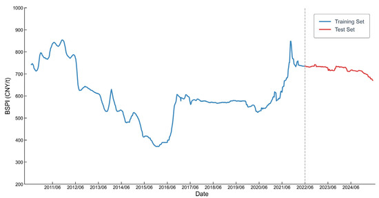
Figure 3.
Historical Trend of the BSPI (June 2010–May 2025).
4.2. Dataset Partitioning and Statistical Features
The dataset is partitioned into training and test sets using an 80:20 split:
- Training Set: The first 588 observations (June 2010–September 2021), used for model training and hyperparameter optimization.
- Test Set: The final 147 observations (October 2021–May 2025), used exclusively for final model performance evaluation.
As shown by the descriptive statistics in Table 1, the training and test sets have significantly different distributions. The training set is more volatile (SD = 119.10) and features diverse market patterns (e.g., bull/bear markets, consolidation), providing a rich sample for learning complex dynamics. In contrast, the test set occupies a new price range with a higher mean (720.23 vs. 599.97) but lower volatility. This distributional “drift”[38] between the sets offers an excellent scenario to test the models’ generalization ability.

Table 1.
Descriptive statistics for the full, training, and test sets of the BSPI.
4.3. Preprocessing Parameter Settings
4.3.1. VMD Parameter Optimization
In VMD parameter optimization, the number of modes (K) has a more dominant effect than the penalty factor (α). We therefore employ a two-step strategy: first determining K, then optimizing α.
- Determination of Modes (K): The selection of K involves a trade-off between decomposition accuracy and economic interpretability, as a larger K improves accuracy but reduces interpretation. To find the optimal value, we identify the “elbow point” on a curve plotting VMD reconstruction error (measured by MSE) against K for a given α. As shown in Figure 4, the marginal improvement in MSE peaks at K = 6. Since this result is consistent across various α values, we select K = 6 as the optimal number of modes.
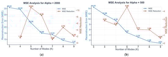 Figure 4. Selection process for the optimal number of VMD modes (K). (a) Results using the default penalty factor of α = 2000; (b) Results for a comparison value of α = 500. The figure displays two representative cases from the six common α values we tested: (500, 1000, 1500, 2000, 2500, and 3000).
 - Optimization of Penalty Factor (α): With K fixed at 6, we test different α values and find that α = 1000 yields the best modal separation, as it produces the clearest spectral boundaries and highest compactness.
Thus, the final parameters for VMD are set to (K = 6, α = 1000).
4.3.2. Data Normalization
All data input to the GRU-Attention models are scaled using max-min normalization to eliminate scale effects and accelerate convergence. To prevent data leakage, the scaler is fitted exclusively on the training set and then applied to normalize the test set and inverse-normalize the final outputs.
4.4. Model Training and Hyperparameter Optimization
4.4.1. Time Series Cross-Validation Strategy
Traditional deep learning models often use a fixed validation set strategy (e.g., 70:15:15 splits); however, this approach is problematic for time-series data like the BSPI with strong temporal characteristics. Specifically, a standard 15% validation set in our data would span from December 2020 to February 2023 (see Figure 3), a unique market phase of unilateral price increases and high-level consolidation, contrasting sharply with the test set’s gentle downward trend. Optimizing hyperparameters on such a validation set could cause overfitting to this specific pattern, yielding poor performance under other market conditions. We verified this experimentally: a model optimized using this fixed validation set exhibited a persistent overestimation bias on the test set, confirming that static validation strategies are unsuitable here.
Therefore, we employ a 3-fold time series cross-validation strategy within the training set. Given the training set’s smaller size (N = 588), a 3-fold split balances sample sufficiency with validation effectiveness. In implementation, the training data is split chronologically into four blocks; for each fold k ∈ {1, 2, 3}, the first k blocks are used for training and block k + 1 for validation. We select the hyperparameters with the best average performance across the three folds.
4.4.2. Hyperparameter Optimization Using Optuna
The Optuna hyperparameter optimization for the GRU-Attention models was configured as follows:
- Objective: Minimize the average MSE over the 3-fold cross-validation. We run 100 trials for each model and select the hyperparameter set with the lowest average MSE.
- Search Space Design:
- GRU: Integer from [16, 192], step 16.
- Dropout rate: Uniformly sampled from [0.1, 0.5].
- Learning rate: Log-uniformly sampled from [1 × 10⁻⁴, 1 × 10⁻²].
- Look-back window: Categorical choice from {2, 4, 8, 13, 15, 25, 49}.
- Fixed Parameters: To balance efficiency and complexity, we use 1 GRU layer and a batch size of 32.
- Look-back Window Design: The window size candidates are chosen based on two factors: (1) standard financial periods, including annual (49 weeks), semi-annual (25 weeks), quarterly (13 weeks), bi-monthly (8 weeks), and monthly (4 weeks); and (2) characteristic periods identified by the VMD (2 and 15 weeks). This design enhances interpretability by incorporating both domain knowledge and data-driven insights.
4.5. Benchmark Models and Ablation Study
We design a systematic benchmark comparison and an ablation study to evaluate our forecasting system’s performance and quantify each core component’s contribution. Table 2 details the configurations of all models.
Table 2.
Overview of Experimental Model Configurations.
4.5.1. Benchmark Models
- ARIMA: A classic linear time-series model used to establish a performance baseline.
- GRU: A standard deep learning model used to verify the advantage of non-linear modeling over linear models.
- GRU-Attention: An advanced single-unit deep learning model used to measure the performance gain of our composite framework over a single model.
4.5.2. Ablation Study
The ablation study progressively builds our framework to systematically verify each module’s effectiveness:
- VMD-Sum: This model independently forecasts each VMD-decomposed mode with GRU-Attention and sums the results. It tests the effectiveness of the decomposition–ensemble strategy against direct forecasting of the original series.
- VMD-Ensemble: Building on VMD-Sum, this model uses a dual-model (ARIMA and GRU-Attention) forecast for each mode, which are then ensembled via our weight optimization strategy. It validates the superiority of this dual-model ensemble over a simple summation of single-model forecasts.
- Hybrid VMD-Ensemble-EC (The Complete Model): This is our final proposed framework, which adds an Error Correction (EC) module to VMD-Ensemble. It is used to validate the contribution of the systematic error correction.
4.6. Experimental Environment
All experiments were conducted in a unified environment to ensure the reproducibility of the results. The hardware configuration was an Intel Core i7-12700H CPU with 32 GB of RAM. The software environment was Python 3.11.9, with core dependency packages including TensorFlow 2.19.0, Keras 3.9.2, Statsmodels 0.14.4, PyVMD 0.2, and Optuna 3.2.1.
5. Results and Discussion
Following our experimental design, this section evaluates the proposed system’s performance in three areas. First, we assess its economic interpretability by analyzing the correspondence between the VMD-decomposed modes and known economic drivers. Second, we evaluate its forecasting accuracy against benchmark models and use an ablation study to quantify each component’s contribution. Finally, we test its robustness and generalization ability under various market conditions.
5.1. VMD: Unifying Technical Effectiveness and Economic Interpretability
Using the optimal parameters (K = 6, α = 1000), VMD decomposes the training set into six Intrinsic Mode Functions (IMFs), as shown in Figure 5. Arranged from lowest to highest frequency, these modes not only denoise and smooth the original series on a technical level but also correspond well with the multi-layered economic drivers of coal prices.
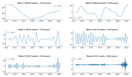
Figure 5.
VMD results for the BSPI training set (IMF1–IMF6).
- Low-Frequency Components: Long-Term Trends & Policy Cycles
- IMF1 delineates the long-term trend driven by macroeconomic fundamentals, with its turning point around 2016 reflecting shifting market expectations from the “New Normal” slowdown to the “Supply-Side Structural Reform.”
- IMF2 represents policy-driven fluctuations. Its peaks and troughs map to key policy impacts: administrative de-capacity in 2016 drove prices up; post-2017 environmental policies suppressed demand; and a post-2021 shift to “energy security” due to pandemic-related supply chain issues again pushed prices higher.
- Mid-Frequency Components: Industrial Rhythms and Seasonality
- IMF3 shows a stable annual cycle, stemming from work schedules around the Spring Festival and annual maintenance in steam coal consuming sectors (e.g., cement, chemicals), creating industrial demand fluctuations independent of power-sector seasonality.
- IMF4 reflects climate-driven seasonality in electricity consumption, with its semi-annual cycle perfectly matching peak demand in summer and winter.
- High-Frequency Components: Market Dynamics and Exogenous Shocks
- IMF5 represents short-term fluctuations, reflecting market participants’ trading strategies based on inventory levels and supply–demand gaps.
- IMF6, a high-frequency irregular component, captures major unpredictable events. Its extreme spikes record structural breaks such as the COVID-19 impact (2020–2021), the geopolitical premium from the war in Ukraine (2022), and the failure of hydropower substitution due to extreme drought (2022).
The VMD results show that the technique not only effectively separates the signal but also produces a frequency-domain partition that is highly consistent with the coal market’s hierarchical economic drivers. By decomposing the price signal into sub-series with clear economic meaning, VMD provides a foundation for building models that are both accurate and interpretable.
5.2. Overall Performance Comparison
Table 3 compares the forecasting performance of the proposed Hybrid VMD-Ensemble-EC model with benchmark models on the test set. The results demonstrate that the proposed model consistently outperforms its benchmarks across all evaluation metrics.
Table 3.
Comparative Performance of Proposed and Benchmark Models.
The proposed model reduces MAPE by 30.8% compared to the standalone GRU-Attention model and by 49.3% relative to the classic ARIMA model, showcasing its ability to effectively handle complex, non-linear series. Moreover, it achieves the lowest Theil’s U statistic (0.5086), indicating substantial improvement over naive forecasts, and the highest DA (49.56%), reflecting its superior capability to capture price movement trends.
To further validate these results, the DM test confirms the robustness of the performance gaps, with p-values for all comparisons significantly below the 0.05 threshold. This provides strong statistical evidence of the proposed model’s superior forecasting accuracy compared to all benchmark models.
5.3. Ablation Analysis: Investigating the Sources of Performance Gain
We conduct a progressive ablation study to quantitatively assess the contribution of each key component. Starting with a baseline GRU-Attention model, we successively add the VMD, ensemble, and error correction modules. The results are presented in Table 4.
Table 4.
Ablation study performance evaluation.
- Introducing VMD (Stage 0 → 1): Adding VMD reduces MAPE by 1.4%, demonstrating its effectiveness in lowering overall error. However, the temporary worsening of Theil’s U (1.0037) and DA (45.62%) underscores the need for subsequent modules to refine forecasts. Importantly, VMD lays the groundwork for tailored ensemble strategies and improved interpretability by decomposing complex series into simpler sub-series.
- Introducing the Dual-Model Weighted Ensemble (Stage 1 → 2): The dual-model ensemble further reduces MAPE by 6.2%, significantly improving Theil’s U (0.7376) and partially recovering DA. This demonstrates the effectiveness of combining complementary models with optimized weights.
Figure 6 illustrates the internal logic of our “tailored” ensemble strategy. The weight optimization process adapts dynamically to modal characteristics: as modal frequency increases (IMF1 → IMF6), the weight for ARIMA decreases, while GRU-Attention gains prominence. This dynamic allocation leverages ARIMA for stable, low-frequency components and GRU-Attention for complex, high-frequency ones, driving the model’s performance gains.
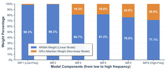
Figure 6.
Adaptive Weight Allocation Based on Frequency. The ensemble assigns higher weights to ARIMA for low-frequency components and GRU-Attention for high-frequency components.
Interestingly, our analysis reveals that ARIMA holds a dominant weight across all modes. However, this does not imply that the modes are inherently linear. This predominance stems from two factors: (1) The BSPI, as a smoothed average price index, reduces short-term fluctuations while amplifying long-term trends, resulting in a time series with strong autocorrelation and trend characteristics that align well with ARIMA’s strength in modeling stable, linear patterns. (2) Our dynamic “coefficient re-estimation” mechanism (Section 3.3.1) enhances ARIMA’s ability to adapt to time-varying dynamics, increasing its forecasting accuracy even for non-linear components.
This analysis highlights that our framework is not a static model combination but rather an intelligent system that adaptively assigns linear or non-linear capabilities based on data complexity. For more volatile daily data, it is reasonable to expect that the weights would naturally shift toward the GRU-Attention model, ensuring robust performance across varying scenarios.
- 3.
- Introducing Error Correction (Stage 2 → 3): The error correction module delivers the largest performance boost, cutting MAPE by 25.1% and achieving the lowest Theil’s U (0.5086) and highest DA (49.56%) across all stages. By addressing systematic biases in residual errors, the module plays a crucial role in optimizing overall performance. The DM test further validates this, showing that the final model (Stage 3) is significantly more accurate than the baseline (Stage 0) and VMD-Sum (Stage 1) models (p < 0.05). Although its performance gain over Stage 2 does not reach conventional statistical significance (p = 0.0546), the error correction module demonstrates a strong trend toward improving accuracy and remains essential for achieving the best overall results.
5.4. Robustness Analysis: Performance Under Different Market Conditions
Figure 7 provides a visual summary of the forecasting performance of all key models across the entire test set. It can be clearly seen that the proposed model’s forecast (Hybrid VMD-Ensemble-EC) tracks the actual price trend more closely than both the benchmark and the intermediate ablation models, visually confirming its superior overall performance.
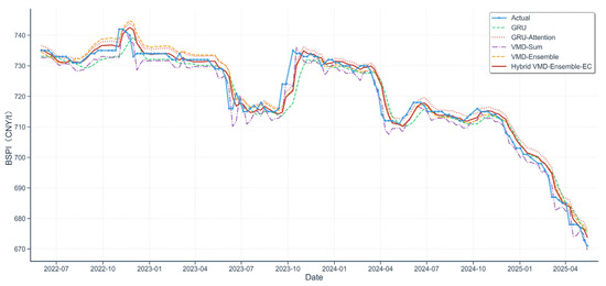
Figure 7.
Visual comparison of forecasts from all key models versus actual values.
To further investigate the model’s robustness, we now analyze its performance in two distinct periods: one of intense volatility (May 2023–January 2024) and one of mild decline (October 2024–May 2025). Detailed forecast curves and performance metrics for these periods are shown in Figure 8 and Table 5, respectively.
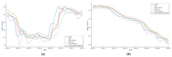
Figure 8.
Forecast comparison of different models during (a) the intense volatility period (May 2023–January 2024) and (b) the mild decline period (October 2024–May 2025).
Table 5.
Comparative model performance under different market conditions.
During the volatile period (Table 5, Figure 8a), the proposed model performs optimally on both RMSE and MAE, and its forecast curve provides the closest fit to the sharp price turning points with minimal lag, demonstrating strong robustness when market uncertainty is high.
Conversely, during the mild decline period, while our model still achieves the best MAE, its RMSE is slightly higher than the structurally simpler VMD-Sum model. Since the RMSE metric penalizes large, sporadic errors more heavily, this result suggests our model is making occasional, significant forecast deviations. Figure 8b helps explain this: the error correction module, ideal for volatility, can “over-correct” in this stable market, causing these large, infrequent errors and thus affecting local forecast stability.
In summary, our model shows good generalization, with its robustness proving especially advantageous in volatile markets. However, the analysis reveals a classic trade-off: the sensitive correction mechanism [39], designed for volatility, can misinterpret noise in stable markets and over-correct. This suggests that, in practice, model selection should be guided by the target market’s volatility characteristics.
6. Conclusions and Future Work
To address the challenge of forecasting complex price series, this study proposes an enhanced “decomposition–forecasting–ensemble–correction” framework and develops a coal price forecasting system based on it. Empirical analysis using BSPI data confirms the system’s superiority over traditional methods, validating the feasibility and effectiveness of the proposed framework.
6.1. Main Conclusions
First, the four-module framework outperforms traditional methods both theoretically and practically. The error correction module effectively addresses a key limitation of traditional “decomposition–ensemble” frameworks by controlling systematic bias. Empirical results validate the Hybrid VMD-Ensemble-EC system’s superiority, as it achieves the lowest errors (MAPE, RMSE, MAE), the best performance relative to a naive forecast (Theil’s U), and the highest accuracy in market direction prediction (DA). The DM test further confirms its statistical advantage over all benchmark models. Ablation studies reveal that the error correction module provides the largest single performance boost, reducing MAPE by 25.1%, underscoring its critical role in overcoming performance bottlenecks in existing methods.
Second, refined design and component synergy are critical for high-performance forecasting. In the decomposition stage, the VMD method not only reduces noise but also connects frequency-domain components to multi-layered economic drivers, enhancing interpretability. During forecasting, the dual-model module achieves an adaptive balance: ARIMA dynamically adjusts parameters to capture linear patterns, while the GRU model, enhanced by an attention mechanism, flexibly processes complex non-linear information. This complementary design improves responsiveness to new data. In the integration stage, a data-driven weight optimization strategy dynamically adjusts the relative contributions of linear and non-linear models to align with data characteristics. Together, these refined methodologies enhance forecasting accuracy while maintaining model simplicity.
Third, an intrinsic trade-off exists between complexity and stability in forecasting models. Robustness analysis shows that while the Hybrid VMD-Ensemble-EC model excels in high-volatility markets by adapting to rapid changes, its accuracy declines in stable conditions due to over-correction. This highlights a key challenge: increasing complexity enhances adaptability but may reduce stability. Balancing this trade-off is crucial for consistent performance across diverse market conditions.
6.2. Limitations of the Model
This study also has certain limitations:
- 1.
- Inability to Support Multi-Step Forecasting
The current error correction mechanism, designed for “instantaneous feedback and rolling correction,” requires the true observation at each time step to adjust the next forecast. While this approach enhances single-step forecasting accuracy, it makes the model heavily dependent on continuous, real-time data. In multi-step scenarios, this correction chain breaks due to the unavailability of future residuals. Consequently, the framework cannot be readily extended to medium- or long-term forecasting tasks.
- 2.
- Data and Feature Constraints
Our study was constrained by data scale, 735 weekly observations is a small sample for deep learning. This led us to select the simpler GRU model over more data-intensive architectures like the Transformer. Furthermore, the model’s current univariate design, which relies solely on historical price data, presents another constraint. Results from the VMD indicate a strong potential correlation between certain modal components and external factors, such as macroeconomic policies and industrial cycles. This suggests that the single-variable input is a potential performance bottleneck and that incorporating multivariate drivers could yield significant improvements.
- 3.
- Limited Component Transparency
Although VMD enhances the framework’s macro interpretability by decomposing complex time series into components aligned with economic drivers, the core predictive units (e.g., GRU-Attention) remain “black boxes,” with their internal decision-making mechanisms still lacking transparency. Introducing mature post hoc explanation techniques, such as Shapley Additive Explanations (SHAP) [40], could enable fine-grained attribution of model predictions. However, this step has not been implemented in the current study and remains a promising direction for future exploration.
6.3. Future Research Prospects
- 1.
- Expanding Data Dimensions and Exploring Advanced Models
Future research can advance in two key directions. First, with the current limited data scale, research can focus on incorporating external information and adopting more robust models. A crucial step is introducing exogenous economic variables (e.g., PMI and industrial output) to enrich the system and upgrade the model from a univariate to a multivariate framework. Non-linear models like SVR can be particularly effective in multivariate scenarios. Additionally, the error correction module can be optimized by leveraging models such as SVR and XGBoost, which are robust to heteroscedasticity [41]. This optimization could replace the current GRU-Attention unit to address the “over-correction” issue observed in low-volatility markets.
Second, as larger datasets become available, more advanced deep learning architectures can be explored. Models like Transformer, which are well-suited for large datasets, could replace the existing GRUs. This would allow for a more effective capture of long-term dependencies in price series and unlock further improvements in model performance.
- 2.
- Deepening Interpretability Research
Model interpretability can be deepened on two complementary levels. Internally, visualizing the attention mechanism’s weights reveals the model’s computational focus, highlighting which parts of the historical sequence it deemed most important. Externally, post hoc tools like SHAP can perform fine-grained attribution, precisely quantifying each input’s contribution to a given prediction. Integrating these ‘process’ and ‘outcome’ perspectives provides a more robust and holistic understanding of the model’s decision-making behavior.
- 3.
- Broadening the Scope of Application
While this study uses coal price forecasting as an empirical case, the four-module framework has broader application potential. Its modular design enables flexible component adjustment based on data characteristics: the GRU-Attention model can be replaced with SVM or Transformer, linear integration can be upgraded to non-linear integration, and decomposition techniques can be substituted as needed. This flexibility allows natural extension to other highly volatile economic forecasting domains, such as liquefied natural gas prices, Bitcoin prices, and shipping indices. Cross-domain applications will validate the framework’s generalizability and provide effective forecasting tools for decision-makers across industries.
Author Contributions
Conceptualization, Q.Q. and L.L.; methodology, Q.Q.; writing—original draft preparation, Q.Q.; writing—review and editing, Q.Q.; visualization, Q.Q.; supervision, L.L.; funding acquisition, Q.Q. All authors have read and agreed to the published version of the manuscript.
Funding
This research was funded by the Postgraduate Education Reform and Quality Improvement Project of Henan Province (Grant no. YJS2025AL50).
Data Availability Statement
The data presented in this study are available upon request from the corresponding author due to the complexity of the algorithm implementation.
Conflicts of Interest
The authors declare no conflicts of interest.
Appendix A
This appendix lists the optimal hyperparameter configurations for the GRU-Attention sub-models. These parameters were independently optimized using Optuna for each of the six modal components generated by VMD.
Table A1.
Optimal Hyperparameters for the GRU-Attention sub-models used in the VMD-Sum and VMD-Ensemble stages.
Table A1.
Optimal Hyperparameters for the GRU-Attention sub-models used in the VMD-Sum and VMD-Ensemble stages.
| Mode | Look-Back | GRUs | Dropout Rate | Learning Rate |
|---|---|---|---|---|
| IMF1 | 4 | 176 | 0.35 | 0.002607 |
| IMF2 | 4 | 128 | 0.20 | 0.001947 |
| IMF3 | 8 | 160 | 0.10 | 0.009414 |
| IMF4 | 4 | 112 | 0.10 | 0.009212 |
| IMF5 | 8 | 160 | 0.10 | 0.009414 |
| IMF6 | 4 | 160 | 0.35 | 0.002620 |
References
- Jones, D. Global Electricity Review 2024; Ember: London, UK, 2024. [Google Scholar]
- Box, G.E.P.; Jenkins, G.M.; Reinsel, G.C.; Ljung, G.M. Time Series Analysis: Forecasting and Control; John Wiley & Sons: Hoboken, NJ, USA, 2015. [Google Scholar] [CrossRef]
- Makridakis, S.; Andersen, A.; Carbone, R.; Fildes, R.; Hibon, M.; Lewandowski, R.; Newton, J.; Parzen, E.; Winkler, R. The accuracy of extrapolation (time series) methods: Results of a forecasting competition. J. Forecast. 1982, 1, 111–153. [Google Scholar] [CrossRef]
- Tsay, R.S. Analysis of Financial Time Series; John Wiley & Sons: Hoboken, NJ, USA, 2005. [Google Scholar] [CrossRef]
- Zhang, G.; Patuwo, B.E.; Hu, M.Y. Forecasting with artificial neural networks: The state of the art. Int. J. Forecast. 1998, 14, 35–62. [Google Scholar] [CrossRef]
- Smola, A.J.; Schölkopf, B. A tutorial on support vector regression. Stat. Comput. 2004, 14, 199–222. [Google Scholar] [CrossRef]
- Bengio, Y.; Simard, P.; Frasconi, P. Learning long-term dependencies with gradient descent is difficult. IEEE Trans. Neural Netw. 1994, 5, 157–166. [Google Scholar] [CrossRef] [PubMed]
- Hochreiter, S.; Schmidhuber, J. Long short-term memory. Neural Comput. 1997, 9, 1735–1780. [Google Scholar] [CrossRef]
- Cho, K.; van Merriënboer, B.; Gulcehre, C.; Bahdanau, D.; Bougares, F.; Schwenk, H.; Bengio, Y. Learning phrase representations using RNN encoder-decoder for statistical machine translation. arXiv 2014, arXiv:1406.1078. [Google Scholar] [CrossRef]
- Vaswani, A.; Shazeer, N.; Parmar, N.; Uszkoreit, J.; Jones, L.; Gomez, A.N.; Kaiser, Ł.; Polosukhin, I. Attention is all you need. Adv. Neural Inf. Process. Syst. 2017, 30, 5998–6008. [Google Scholar]
- Taylor, S.J.; Letham, B. Forecasting at scale. Am. Stat. 2018, 72, 37–45. [Google Scholar] [CrossRef]
- Li, X.; Sengupta, T.; Si Mohammed, K.; Jamaani, F. Forecasting the lithium mineral resources prices in China: Evidence with Facebook Prophet (Fb-P) and Artificial Neural Networks (ANN) methods. Resour. Policy 2023, 82, 103580. [Google Scholar] [CrossRef]
- Mitchell, T.M. Machine Learning; McGraw-Hill: Columbus, OH, USA, 1997. [Google Scholar]
- Adadi, A.; Berrada, M. Peeking inside the black-box: A survey on explainable artificial intelligence (XAI). IEEE Access. 2018, 6, 52138–52160. [Google Scholar] [CrossRef]
- Wu, Z.; Huang, N.E. Ensemble empirical mode decomposition: A noise-assisted data analysis method. Adv. Adapt. Data Anal. 2009, 1, 1–41. [Google Scholar] [CrossRef]
- Dragomiretskiy, K.; Zosso, D. Variational mode decomposition. IEEE Trans. Signal Process. 2014, 62, 531–544. [Google Scholar] [CrossRef]
- Yu, L.; Wang, Z.; Tang, L. A decomposition–ensemble model with data-characteristic-driven reconstruction for crude oil price forecasting. Appl. Energy. 2015, 156, 251–267. [Google Scholar] [CrossRef]
- Meng, E.; Huang, S.; Huang, Q.; Fang, W.; Wang, H.; Leng, G.; Liang, H. A hybrid VMD-SVM model for practical streamflow prediction using an innovative input selection framework. Water Resour. Manag. 2021, 35, 1321–1337. [Google Scholar] [CrossRef]
- Zhao, L.; Li, Z.; Qu, L.; Zhang, J.; Teng, B. A hybrid VMD-LSTM/GRU model to predict non-stationary and irregular waves on the east coast of China. Ocean Eng. 2023, 287, 114136. [Google Scholar] [CrossRef]
- Bates, J.M.; Granger, C.W.J. The combination of forecasts. J. Oper. Res. Soc. 1969, 20, 451–468. [Google Scholar] [CrossRef]
- Wolpert, D.H. Stacked generalization. Neural Netw. 1992, 5, 241–259. [Google Scholar] [CrossRef]
- Domingos, P. A unified bias-variance decomposition and its applications. In Proceedings of the 17th International Conference on Machine Learning, San Francisco, CA, USA, 29 June—2 July 2000; University of Washington: Seattle, WA, USA, 2000; pp. 231–238. [Google Scholar]
- Granger, C.W.; Morris, M.J. Time series modelling and interpretation. J. R. Stat. Soc. Ser. A Gen. 1976, 139, 246–257. [Google Scholar] [CrossRef]
- Friedman, J.H. Greedy function approximation: A gradient boosting machine. Ann. Stat. 2001, 29, 1189–1232. [Google Scholar] [CrossRef]
- Khashei, M.; Bijari, M. A novel hybridization of artificial neural networks and ARIMA models for time series forecasting. Appl. Soft Comput. 2010, 11, 2664–2675. [Google Scholar] [CrossRef]
- Pai, P.F.; Lin, C.S. A hybrid ARIMA and support vector machines model in stock price forecasting. Omega 2005, 33, 497–505. [Google Scholar] [CrossRef]
- Livieris, I.E.; Pintelas, E.; Pintelas, P. A CNN–LSTM model for gold price time-series forecasting. Neural Comput. Appl. 2020, 32, 17351–17360. [Google Scholar] [CrossRef]
- Yu, L.; Wang, S.; Lai, K.K. Forecasting crude oil price with an EMD-based neural network ensemble learning paradigm. Energy Econ. 2008, 30, 2623–2635. [Google Scholar] [CrossRef]
- Bahdanau, D.; Cho, K.; Bengio, Y. Neural machine translation by jointly learning to align and translate. arXiv 2014, arXiv:1409.0473. [Google Scholar]
- Luong, M.-T.; Pham, H.; Manning, C.D. Effective approaches to attention-based neural machine translation. In Proceedings of the 2015 Conference on Empirical Methods in Natural Language Processing, Lisbon, Portugal, September 2015; pp. 1412–1421. [Google Scholar] [CrossRef]
- Makridakis, S.; Hibon, M. The M3-Competition: Results, conclusions and implications. Int. J. Forecast. 2000, 16, 451–476. [Google Scholar] [CrossRef]
- Akiba, T.; Sano, S.; Yanase, T.; Ohta, T.; Koyama, M. Optuna: A Next-generation Hyperparameter Optimization Framework. In Proceedings of the 25th ACM SIGKDD International Conference on Knowledge Discovery & Data Mining, Anchorage, AK, USA, 4–8 August 2019; pp. 2623–2631. [Google Scholar] [CrossRef]
- Bergstra, J.; Bardenet, R.; Bengio, Y.; Kégl, B. Algorithms for hyper-parameter optimization. Adv. Neural Inf. Process. Syst. 2011, 24. [Google Scholar]
- Li, L.; Jamieson, K.; DeSalvo, G.; Rostamizadeh, A.; Talwalkar, A. Hyperband: A novel bandit-based approach to hyperparameter optimization. J. Mach. Learn. Res. 2017, 18, 6765–6816. [Google Scholar]
- Zhang, Y.; Liu, D.; Wang, L. A novel hybrid model for crude oil price forecasting based on VMD and GRU. Energy 2021, 214, 118931. [Google Scholar]
- Li, C.; Chen, Z.; Li, M.; Liu, Y. A hybrid approach for wind power forecasting based on variational mode decomposition and long short-term memory networks. J. Clean. Prod. 2020, 259, 120857. [Google Scholar] [CrossRef]
- Zhang, K.; Cao, H.; Thé, J.; Yu, H. A hybrid model for multi-step coal price forecasting using decomposition technique and deep learning algorithms. Appl. Energy. 2022, 306, 118011. [Google Scholar] [CrossRef]
- Moreno-Torres, J.G.; Raeder, T.; Alaiz-Rodríguez, R.; Chawla, N.V.; Herrera, F. A unifying view on dataset shift in classification. Pattern Recognit. 2012, 45, 521–530. [Google Scholar] [CrossRef]
- Geman, S.; Bienenstock, E.; Doursat, R. Neural networks and the bias/variance dilemma. Neural Comput. 1992, 4, 1–58. [Google Scholar] [CrossRef]
- Lundberg, S.M.; Lee, S.I. A unified approach to interpreting model predictions. Adv. Neural Inf. Process. Syst. 2017, 30, 4765–4774. [Google Scholar]
- Chen, T.; Guestrin, C. XGBoost: A scalable tree boosting system. In Proceedings of the 22nd ACM SIGKDD International Conference on Knowledge Discovery and Data Mining, San Francisco, CA, USA, 13–17 August 2016; pp. 785–794. [Google Scholar] [CrossRef]
Disclaimer/Publisher’s Note: The statements, opinions and data contained in all publications are solely those of the individual author(s) and contributor(s) and not of MDPI and/or the editor(s). MDPI and/or the editor(s) disclaim responsibility for any injury to people or property resulting from any ideas, methods, instructions or products referred to in the content. |
© 2025 by the authors. Licensee MDPI, Basel, Switzerland. This article is an open access article distributed under the terms and conditions of the Creative Commons Attribution (CC BY) license (https://creativecommons.org/licenses/by/4.0/).