Article

A Symmetric Quantum Perspective of Analytical Inequalities and Their Applications

by
Muhammad Zakria Javed
1,
Nimra Naeem
1,
Muhammad Uzair Awan
1,
Yuanheng Wang
2,* and
Omar Mutab Alsalami
3
1
Department of Mathematics, Government College University Faisalabad, Faisalabad 38000, Pakistan
2
School of Mathematical Sciences, Zhejiang Normal University, Jinhua 321004, China
3
Department of Electrical Engineering, College of Engineering, Taif University, P.O. Box 11099, Taif 21944, Saudi Arabia
*
Author to whom correspondence should be addressed.
Mathematics 2025, 13(18), 2910; https://doi.org/10.3390/math13182910
Submission received: 5 August 2025 / Revised: 2 September 2025 / Accepted: 5 September 2025 / Published: 9 September 2025
(This article belongs to the Special Issue Mathematical Inequalities and Fractional Calculus)

Abstract

This study explores some new symmetric quantum inequalities that are based on Breckner’s convexity. By using these concepts, we propose new versions of Hermite–Hadamard (H-H) and Fejer-type inequalities. Additionally, we establish a new integral identity which helped us to derive a set of new quantum inequalities. Using the symmetric quantum identity, Breckner’s convexity, and several other classical inequalities, we develop blended bounds for a general quadrature scheme. To ensure the significance of this study, a few captivating applications are discussed.

1. Introduction

Mathematical analysis comprises various concepts and domains, including inequalities. This subject is regarded as fundamental to analysis; due to its governing role, researchers have focused on generalizing the existing concepts, expanding the applicable domain according to the requirements of modern-day mathematics. They are classified as dynamical and analytical inequalities, where dynamical inequalities are beneficial for studying the uniqueness and stability of solutions of dynamical systems. Analytical inequalities encompass the classical inequalities and error inequalities of quadrature procedures and algorithms. This subject is explored through diverse strategies, including convex analysis. In the expansion of inequalities, the substantial role of convexity is unprecedented because the development of various fundamental inequalities and their robust refinements can be recovered by leveraging the notion of convex mappings. Let’s explore this topic further:
Definition 1 ([1]).
A real valued mapping defined over convex set C is said to be convex if
T ( ( 1 β ) ϱ 1 + β ϱ 2 ) T ( ϱ 1 ) + β ( T ( ϱ 2 ) T ( ϱ 1 ) ) , β [ 0 , 1 ] a n d ϱ 1 , ϱ 2 C .
Next, we give the notion of Breckner’s convexity.
Definition 2 ([2]).
A real valued mapping defined over convex set C is said to be Breckner’s convex if
T ( ( 1 β ) ϱ 1 + β ϱ 2 ) ( 1 β ) ϑ T ( ϱ 1 ) + β ϑ T ( ϱ 2 ) , β [ 0 , 1 ] , ϑ ( 0 , ) , a n d ϱ 1 , ϱ 2 C .
The first fundamental inequality associated with Breckner’s convex mapping is Jensen’s inequality, and is given as
Theorem 1 ([2]).
If  T : [ ϱ 1 , ϱ 2 ] R is a Breckner convex mapping, then
T i = 1 δ β i ϕ i i = 1 δ β i ϑ T ( ϕ i ) , i = 1 δ β i = 1 , ϑ > 0 , a n d ϕ i [ ϱ 1 , ϱ 2 ] .
It is obvious that the above inequality is the simple extension of classical convexity for δ -different nodes. For more details, see [1,3,4]. Exploring the convex inequalities, another useful double inequality, which serves as a criteria to observe the concavity of mappings, is known as Hermite–Hadamard’s inequality.
Theorem 2 ([5]).
Let T : [ ϱ 1 , ϱ 2 ] R be a Breckner’s convex mapping; then,
( ϱ 2 ϱ 1 ) T ( ϱ 1 ) + T ( ϱ 2 ) ϑ + 1 ϱ 1 ϱ 2 T ( β ) d β ( ϱ 2 ϱ 1 ) 2 ϑ 1 T ϱ 1 + ϱ 2 2 ,
where ϑ > 0 .
Its weighted form associated with symmetric mappings is given as
Theorem 3 ([6]).
If T : [ ϱ 1 , ϱ 2 ] R is a Breckner convex mapping and V is a symmetric mapping about ϱ 1 + ϱ 2 2 , then
T ( ϱ 1 ) + T ( ϱ 2 ) 2 ϱ 1 ϱ 2 ϱ 2 β ϱ 2 ϱ 1 ϑ + β ϱ 1 ϱ 2 ϱ 1 ϑ V ( β ) d β ϱ 1 ϱ 2 T ( β ) V ( β ) d β 2 ϑ 1 T ϱ 1 + ϱ 2 2 ϱ 1 ϱ 2 V ( β ) d β .
For constant V ( β ) = 1 and ϑ = 1 , the aforementioned inequality reduces to the classical H-H inequality. For comprehensive details, consult [7,8,9,10].
Now we look at Simpson’s error inequality.
Theorem 4 ([11]).
If T : [ ϱ 1 , ϱ 2 ] R is fourth-order continuously differentiable mapping and T ( 4 ) : = sup β ( ϱ 1 , ϱ 2 ) T ( 4 ) ( β ) < , then
1 3 T ( ϱ 1 ) + T ( ϱ 2 ) 2 + 2 T ϱ 1 + ϱ 2 2 1 ϱ 2 ϱ 1 ϱ 1 ϱ 2 T ( β ) d β 1 2880 T ( 4 ) ( ϱ 2 ϱ 1 ) 4 .
Next, we report the Simpson’s inequality associated with Breckner’s convexity.
Theorem 5 ([12]).
Let T : [ ϱ 1 , ϱ 2 ] R be a differentiable mapping and | T | be a Breckner convex mapping; then, the following inequality holds:
1 6 T ( ϱ 1 ) + 4 T ϱ 1 + ϱ 2 2 + T ( ϱ 2 ) 1 ϱ 2 ϱ 1 ϱ 1 ϱ 2 T ( β ) d β ( ϱ 2 ϱ 1 ) 6 ϑ 9 · 2 ϑ + 5 ϑ + 2 · 6 ϑ + 3 ϑ 12 18 ( ϑ 2 + 3 ϑ + 2 ) T ( ϱ 1 ) + T ( ϱ 2 ) .
In the eighteenth century, Euler discussed the two renowned types of calculus named as q 1 and h calculus. Both solely depend on discrete approaches. Derivatives and anti-derivatives incorporated with q 1 differences are the principal tools of quantum calculus. In the early twentieth century, Jackson’s investigations on q 1 calculus motivated the researchers to focus on these operators. One of the principle perspectives was to discuss the non-differentiable mappings. Working within this general setup, researchers utilized their efforts to establish the q 1 analogues of various existing concepts of special mappings, number theory, inequalities, difference equations, differential geometry, etc. Recently, researchers formulated the q 1 variants of fractional and several other useful environments.
In [13], the authors utilized the left end point of the interval and defined the finite interval quantum derivative.
Definition 3 ([13]).
Let T : [ ϱ 1 , ϱ 2 ] R be a mapping. Then, the left quantum operator is stated as
D q 1 ϱ 1 T β = T β T q 1 β + 1 q 1 ϱ 1 1 q 1 β ϱ 1 , β ϱ 1 a n d D q 1 ϱ 1 T ϱ 1 = lim β ϱ 1 D q 1 ϱ 1 T β ,
where 0 < q 1 < 1 .
Likewise, the representation of the left q 1 -definite integral is stated as
Definition 4 ([13]).
Let T : [ ϱ 1 , ϱ 2 ] R R be an arbitrary mapping. Then,
ϱ 1 ϱ 2 T ( ϱ 1 ) d q 1 ϱ 1 β = ( 1 q 1 ) ( ϱ 2 ϱ 1 ) δ = 0 q 1 δ T ( q 1 δ ϱ 2 + ( 1 q 1 δ ) ϱ 1 ) .
Note that if ϱ 1 = 0 , then we have the classical q 1 -integral, which is defined as
0 β T ( β ) d q 1 β = ( 1 q 1 ) β δ = 0 q 1 δ T ( q 1 δ β ) .
The correct q 1 -trapezoidal inequality was proved by Alp et al. [14].
Theorem 6 ([14]).
For 0 < q 1 < 1 and a convex mapping T : [ ϱ 1 , ϱ 2 ] R on ( ϱ 1 , ϱ 2 ) . The q 1 HHI is
T q 1 ϱ 1 + ϱ 2 1 + q 1 1 ϱ 2 ϱ 1 ϱ 1 ϱ 2 T ( μ ) ϱ 1 d q 1 μ q 1 T ( ϱ 1 ) + T ( ϱ 2 ) 1 + q 1 .
The right q 1 operators are defined as follows:
Definition 5 ([15]).
Let T : [ ϱ 1 , ϱ 2 ] R be a mapping. Then left quantum operator is stated as
D q 1 ϱ 2 T β = T q 1 β + 1 q 1 ϱ 2 T β 1 q 1 ϱ 2 β , β ϱ 2 a n d D q 1 ϱ 2 T ϱ 2 = lim β ϱ 2 D q 1 ϱ 2 T β ,
where 0 < q 1 < 1 .
The integral operator is defined as
Definition 6 ([15]).
Let T : [ ϱ 1 , ϱ 2 ] R R be an arbitrary mapping. Then, the q 1 integral on [ ϱ 1 , ϱ 2 ] is defined as
ϱ 1 ϱ 2 T ( β ) d q 1 ϱ 2 β = ( 1 q 1 ) ( ϱ 2 ϱ 1 ) δ = 0 q 1 δ T ( q 1 δ ϱ 1 + ( 1 q 1 δ ) ϱ 2 ) .
Symmetric derivatives were developed to study non-differentiable absolute mappings. Note that they do not reduce to classical operators. Noticing the significance of symmetric calculus, Da Cruz et al. [16] worked on the q 1 -forms of symmetric derivative and integral operators in Jackson’s sense. Also, they have discussed the results associated with the calculus of variation.
In 2024, Bilal et al. [17] purported the idea of a symmetric quantum calculus following the technique of Tariboon and his fellows.
Definition 7 ([17]).
Let T : J R be a mapping and 0 < q 1 < 1 ; then,
D q 1 s ϱ 1 T ( β ) = T ( q 1 1 β + ( 1 q 1 1 ) ϱ 1 ) T ( q 1 β + ( 1 q 1 ) ϱ 1 ) ( q 1 1 q 1 ) ( β ϱ 1 ) , β ϱ 1 .
And D q 1 s ϱ 1 T ( ϱ 1 ) = lim q 1 1 D q 1 s ϱ 1 T ( β ) , if the limit exists. If ϱ 1 = 0 , then D q 1 s ϱ 1 T = D q 1 s T .
Likewise, the symmetric q 1 definite integral is described as
Definition 8 ([17]).
Let T : J R be a mapping and 0 < q 1 < 1 . Then,
ϱ 1 ϱ 2 T ( β ) d q 1 s ϱ 1 β = ( ϱ 2 ϱ 1 ) ( q 1 1 q 1 ) δ = 0 q 1 2 δ + 1 T ( q 1 2 δ + 1 ϱ 2 + ( 1 q 1 2 δ + 1 ) ϱ 1 ) = ( ϱ 2 ϱ 1 ) ( 1 q 1 2 ) δ = 0 q 1 2 δ T ( q 1 2 δ + 1 ϱ 2 + ( 1 q 1 2 δ + 1 ) ϱ 1 ) .
The right symmetric operators are given in [18].
Definition 9 ([18]).
Let T : J R be a mapping and 0 < q 1 < 1 . Then,
D q 1 s ϱ 2 T ( β ) = T ( q 1 β + ( 1 q 1 ) ϱ 2 ) T ( q 1 1 β + ( 1 q 1 1 ) ϱ 2 ) ( q 1 1 q 1 ) ( ϱ 2 β ) , β ϱ 2 .
and D q 1 s ϱ 2 T ( ϱ 2 ) = lim q 1 1 D q 1 s ϱ 2 T ( β ) , if limit exist. If ϱ 2 = 0 then D q 1 s ϱ 2 T = D q 1 s T .
Definition 10 ([18]).
Let T : J R be a mapping and 0 < q 1 < 1 . Then,
ϱ 1 ϱ 2 T ( β ) d q 1 s ϱ 2 β = ( ϱ 2 ϱ 1 ) ( q 1 1 q 1 ) δ = 0 q 1 2 δ + 1 T ( q 1 2 δ + 1 ϱ 1 + ( 1 q 1 2 δ + 1 ) ϱ 2 ) = ( ϱ 2 ϱ 1 ) ( 1 q 1 2 ) δ = 0 q 1 2 δ T ( q 1 2 δ + 1 ϱ 1 + ( 1 q 1 2 δ + 1 ) ϱ 2 ) .
The right symmetric q 1 integral of a mapping T exits if δ = 0 q 1 2 δ + 1 T ( q 1 2 δ + 1 ϱ 1 + ( 1 q 1 2 δ + 1 ) ϱ 2 ) converges.
Theorem 7 ([18]).
Suppose that T : J R is a convex mapping and 0 < q 1 < 1 . Then,
T ϱ 1 + ϱ 2 2 1 2 ( ϱ 2 ϱ 1 ) ϱ 1 ϱ 2 T ( β ) d q 1 s ϱ 1 β + ϱ 1 ϱ 2 ϕ ( β ) d q 1 s ϱ 2 β ϕ ( ϱ 1 ) + ϕ ( ϱ 2 ) 2 .
Tariboon and Ntouyas [13] explored the left endpoint-based finite interval quantum calculus and discussed the several intrinsic properties. Furthermore, they examined q 1 -impulsive difference equations. In [19], Sudsutad et al. utilized the quantum framework to investigate the various classical inequalities. In [20], the authors established the right estimates of the q 1 -trapezium inequality. Alp et al. [14] presented the new trapezium-type q 1 -trapezium-type integral inequalities through a geometrical approach and several error inequalities. Kunt et al. [15] studied the right- q 1 -operators along with important characterization and provided an alternative approach to discuss the various problems. Kunt et al. [21] focused on the development of the q 1 -Montgomery identity and related Ostrowski-like inequalities. In Bin-Mohsin et al. [22] worked on Milne–Mercer-like inequalities, incorporating q 1 -calculus. Ali et al. [23] analyzed both left and right estimates of trapezium inequalities, respectively. Khan et al. [24] examined Hadamard’s inequalities utilizing the Green mappings-based identities for twice q 1 -differentiable mappings. Saleh et al. [25] discussed the q 1 -versions of error inequalities of the dual Simpson’s scheme via convexity. Du et al. [26] bridged the concepts of quantum calculus, parametric approaches, and the convexity of mappings to construct new unified bounds. In [27], the authors looked at majorized inequalities via q 1 -differentiable convex mappings. For more details, see [28].
In 2023, Bilal et al. [17] followed the strategy of [13] and defined the idea of left symmetric quantum operators. Furthermore, they looked at the symmetric quantum form of existing classical inequalities. Nosheen et al. [29] investigated some of Hadamard’s inequalities, leveraging the concept of a newly developed calculus in [17]. Vivas-Cortez [18] comprehensively studied both left and right symmetric quantum operators to formulate new counterparts of inequalities. Butt et al. [30] discussed the two-dimensional symmetric operators to analyze the coordinated inequalities pertaining to convexity. Liu et al. [31] utilized symmetric quantum operators to prove new refinements of H-H’s type inequalities and error analysis of general quadrature rules through a unified approach. For further detail, see [32,33].
Motivation: It is a known fact that the significance and utility of inequalities developed for convex mappings illustrate the necessity of inequalities for non-convex mappings. Among the non-convex mappings is Breckner’s convexity, which unifies the classical and several other kinds of mappings. The extensive work on Bruckner’s convexity in the literature highlights the scope of this class.
Following the recent developments, we found some gaps in understanding:
  • What are the estimates of the symmetric quantum average integral for ϑ convex mappings?
  • What is the weighted form of symmetric quantum HH inequality via symmetric mappings?
  • Development of unified error approximations of quadrature procedures pertaining to Breckner’s convexity.
Structure and significance: The following study is organized to resolve the abovementioned problems in four different parts. Initially, we will provide a required review of the literature, a statement of the problem, and an explanation of the need for this study. In the forthcoming section, we will prove some new symmetric quantum refinements of HH for generalized convexity along with their numerical and visual confirmations. Next, an auxiliary unified symmetric quantum identity and related error approximations will be presented. Some new robust deductions for the main results will be mentioned. Finally, to ensure the significance, a few interesting applications will be offered.
This study is novel due to its generic nature, because a blend of symmetric quantum inequalities are studied identically. Moreover, the obtained results are valid for a wide range of mapping classes, which makes them significant and essential to study within this framework.

2. Main Results

This section contains some novel versions of Hermite–Hadamard’s and parameterized inequalities involving Breckner’s convexity in the setting of symmetric quantum calculus.

2.1. Symmetric Quantum Hermite–Hadamard’s Inequality

First, we give a novel Hadamard inequality.
Theorem 8.
Let T : I R be a Breckner’s convex mapping and 0 < q 1 < 1 . Then,
2 ϑ T ϱ 1 + ϱ 2 2 1 ( ϱ 2 ϱ 1 ) ϱ 1 ϱ 2 T ( β ) ϱ 2 d q 1 s β + ϱ 1 ϱ 2 T ( β ) ϱ 1 d q 1 s β T ( ϱ 1 ) + T ( ϱ 2 ) 1 [ ϑ + 1 ] q 1 , s + 0 1 ( 1 β ) 0 ϑ d q 1 s β ,
where ϑ > 0 .
Proof. 
Since T is Breckner’s convex mapping, then
2 ϑ T ϱ 1 + ϱ 2 2 T ( β ϱ 1 + ( 1 β ) ϱ 2 ) + T ( ( 1 β ) ϱ 1 + β ϱ 2 )
Applying the q 1 -symmetric integral on both sides of the above inequality
2 ϑ T ϱ 1 + ϱ 2 2 0 1 T ( β ϱ 1 + ( 1 β ) ϱ 2 ) 0 d q 1 s β + 0 1 T ( ( 1 β ) ϱ 1 + β ϱ 2 ) 0 d q 1 s β = 1 ϱ 2 ϱ 1 ϱ 1 ϱ 2 T ( β ) ϱ 2 d q 1 s β + 1 ( ϱ 2 ϱ 1 ) ϱ 1 ϱ 2 T ( β ) ϱ 1 d q 1 s β .
Finally, we get
2 ϑ T ϱ 1 + ϱ 2 2 1 ( ϱ 2 ϱ 1 ) ϱ 1 ϱ 2 T ( β ) ϱ 2 d q 1 s β + ϱ 1 ϱ 2 T ( β ) ϱ 1 d q 1 s β .
Next, we prove our second inequality by utilizing Breckner’s convexity
T ( β ϱ 1 + ( 1 β ) ϱ 2 ) β ϑ T ( ϱ 1 ) + ( 1 β ) ϑ T ( ϱ 2 ) ,
and
T ( ( 1 β ) ϱ 1 + β ϱ 2 ) ( 1 β ) ϑ T ( ϱ 1 ) + β ϑ T ( ϱ 2 ) .
Adding (1) and (2), and taking the q 1 integral on both sides
0 1 T ( β ϱ 1 + ( 1 β ) ϱ 2 ) + T ( ( 1 β ) ϱ 1 + β ϱ 2 ) 0 d q 1 s β T ( ϱ 1 ) + T ( ϱ 2 ) 0 1 β ϑ + ( 1 β ) ϑ 0 d q 1 s β .
This implies that
1 ( ϱ 2 ϱ 1 ) ϱ 1 ϱ 2 T ( β ) ϱ 2 d q 1 s β + ϱ 1 ϱ 2 T ( β ) ϱ 1 d q 1 s β ( T ( ϱ 1 ) + T ( ϱ 2 ) ) 1 [ ϑ + 1 ] q 1 , s + 0 1 ( 1 β ) 0 s d q 1 s β .
This ends the proof. □
Corollary 1.
Inserting ϑ = 1 in Theorem 8, we get the symmetric quantum Hermite–Hadamard inequality, which is given in [18].
2 T ϱ 1 + ϱ 2 2 1 ( ϱ 2 ϱ 1 ) ϱ 1 ϱ 2 T ( β ) ϱ 2 d q 1 s β + ϱ 1 ϱ 2 T ( β ) ϱ 1 d q 1 s β T ( ϱ 1 ) + T ( ϱ 2 ) .
Example 1.
Let T : [ ϱ 1 , ϱ 2 ] R be a Breckner convex mapping meeting all the conditions of Theorem 8, and defined as T ( β ) = β 2 , ϱ 1 = 0 and ϱ 2 = 2 . Then,
2 q 1 q 1 4 16 q 1 2 1 + q 1 2 + q 1 4 16 q 1 1 + q 1 2 + 8 4 q 1 .
Figure 1 presents a graphical breakdown of the sides of Theorem 8. Also, the red, purple, and green colors represent the middle and left- and right-sided terms of Theorem 8, respectively.

2.2. Hermite–Hadamard–Fejér Inequality

Now, we prove the weighted Hadamard inequality pertaining to Breckner’s convexity.
Theorem 9.
Let T : [ ϱ 1 , ϱ 2 ] R be a Breckner convex mapping and V be a symmetric mapping about ϱ 1 + ϱ 2 2 . Then,
2 ϑ 1 T ϱ 1 + ϱ 2 2 ϱ 1 ϱ 2 V ( β ) ϱ 1 d q 1 s β + ϱ 1 ϱ 2 V ( β ) ϱ 2 d q 1 s β ϱ 1 ϱ 2 T ( β ) V ( β ) ϱ 1 d q 1 s β + ϱ 1 ϱ 2 T ( β ) V ( β ) ϱ 2 d q 1 s β ( ϱ 2 ϱ 1 ) T ( ϱ 1 ) + T ( ϱ 2 ) 2 0 1 V ( β ϱ 1 + ( 1 β ) ϱ 2 ) + V ( ( 1 β ) ϱ 1 + β ϱ 2 ) ] [ β ϑ + ( 1 β ) ϑ 0 d q 1 s β ,
where 0 < q 1 < 1 and ϑ > 0 .
Proof. 
Let T be a Breckner convex mapping; then,
2 ϑ T ϱ 1 + ϱ 2 2 T ( β ϱ 1 + ( 1 β ) ϱ 2 ) + T ( ( 1 β ) ϱ 1 + ϱ 2 ) .
Multiply both sides of the aforementioned inequality by V ( β ϱ 1 + ( 1 β ) ϱ 2 ) and taking q 1 -integration on both sides, we have
2 ϑ T ϱ 1 + ϱ 2 2 0 1 V ( β ϱ 1 + ( 1 β ) ϱ 2 ) 0 d q 1 s β 0 1 T ( β ϱ 1 + ( 1 β ) ϱ 2 ) V ( β ϱ 1 + ( 1 β ) ϱ 2 ) 0 d q 1 s β + 0 1 T ( ( 1 β ) ϱ 1 + β ϱ 2 ) V ( β ϱ 1 + ( 1 β ) ϱ 2 ) 0 d q 1 s β .
Since V is symmetric about ϱ 1 + ϱ 2 2 , then V ( β ϱ 1 + ( 1 β ) ϱ 2 ) = V ( ( 1 β ) ϱ 1 + β ϱ 2 ) ,
2 ϑ 1 T ϱ 1 + ϱ 2 2 ϱ 1 ϱ 2 V ( β ) ϱ 1 d q 1 s β + ϱ 1 ϱ 2 V ( β ) d q 1 s ϱ 2 β ϱ 1 ϱ 2 T ( β ) V ( β ) ϱ 1 d q 1 s β + ϱ 1 ϱ 2 T ( β ) V ( β ) d q 1 s ϱ 2 β .
To prove the second part, we again consider Breckner’s convexity property.
T ( β ϱ 1 + ( 1 β ) ϱ 2 ) V ( β ϱ 1 + ( 1 β ) ϱ 2 ) + T ( ( 1 β ) ϱ 1 + β ϱ 2 ) V ( ( 1 β ) ϱ 1 + β ϱ 2 ) [ β ϑ + ( 1 β ) ϑ ] [ T ( ϱ 1 ) + T ( ϱ 2 ) ] V ( β ϱ 1 + ( 1 β ) ϱ 2 ) .
Again considering the symmetric quantum integration, we get
0 1 T ( β ϱ 1 + ( 1 β ) ϱ 2 ) V ( β ϱ 1 + ( 1 β ) ϱ 2 ) 0 d q 1 s β + 0 1 T ( ( 1 β ) ϱ 1 + β ϱ 2 ) V ( ( 1 β ) ϱ 1 + β ϱ 2 ) 0 d q 1 s β [ T ( ϱ 1 ) + T ( ϱ 2 ) ] V ( β ϱ 1 + ( 1 β ) ϱ 2 ) 0 1 [ β ϑ + ( 1 β ) ϑ ] 0 d q 1 s β .
This implies that
2 ϑ 1 T ϱ 1 + ϱ 2 2 ϱ 1 ϱ 2 V ( β ) ϱ 1 d q 1 s β + ϱ 1 ϱ 2 V ( β ) ϱ 2 d q 1 s β ϱ 1 ϱ 2 T ( β ) V ( β ) ϱ 1 d q 1 s β + ϱ 1 ϱ 2 T ( β ) V ( β ) ϱ 2 d q 1 s β ( ϱ 2 ϱ 1 ) T ( ϱ 1 ) + T ( ϱ 2 ) 2 0 1 V ( β ϱ 1 + ( 1 β ) ϱ 2 ) + V ( ( 1 β ) ϱ 1 + β ϱ 2 ) β ϑ + ( 1 β ) ϑ 0 d q 1 s β .
Finally, we get our desired inequality. □
Corollary 2.
For ϑ = 1 in Theorem 8, we get symmetric quantum Hermite–Hadamard–Fejer inequality.
T ϱ 1 + ϱ 2 2 ϱ 1 ϱ 2 V ( β ) ϱ 1 d q 1 s β + ϱ 1 ϱ 2 V ( β ) ϱ 2 d q 1 s β ϱ 1 ϱ 2 T ( β ) V ( β ) ϱ 1 d q 1 s β + ϱ 1 ϱ 2 T ( β ) V ( β ) ϱ 2 d q 1 s β ( ϱ 2 ϱ 1 ) T ( ϱ 1 ) + T ( ϱ 2 ) 2 0 1 V ( β ϱ 1 + ( 1 β ) ϱ 2 ) + V ( ( 1 β ) ϱ 1 + β ϱ 2 ) 0 d q 1 s β .
Example 2.
Let T : [ ϱ 1 , ϱ 2 ] R be a Breckner convex mapping meeting all the conditions of Theorem 8 and is defined as T ( β ) = β 2 and V ( β ) = ( β 1 ) 2 , ϱ 1 = 0 and ϱ 2 = 2 . Then,
16 q 1 2 1 + q 1 2 + q 1 4 16 q 1 1 + q 1 2 + 4 32 q 1 2 1 + q 1 2 + q 1 4 + q 1 6 + q 1 8 32 q 1 3 1 + q 1 2 + q 1 4 + q 1 6 + 16 q 1 2 1 + q 1 2 + q 1 4 + 32 ( 1 q 1 ) 3 ( 1 + q 1 ) 4 32 ( 1 q 1 ) 3 ( 1 + q 1 ) 3 16 q 1 1 + q 1 2 + 8 4 16 q 1 2 1 + q 1 2 + q 1 4 16 q 1 1 + q 1 2 + 4 .
Figure 2 presents a graphical breakdown of the sides of Theorem 9. Also, the red, purple, and green colors represent the middle and left- and right-sided terms of Theorem 9, respectively.

2.3. Symmetric Quantum Differentiable Generic Identity

Now, we derive the parametric identity incorporating with symmetric quantum differentiable mappings.
Lemma 1.
Let T : I R be a continuous and q 1 -differentiable symmetric mapping on I with 0 < q 1 < 1 . Then, the identity
λ ( 1 μ ) T ( ϱ 1 ) + λ μ T ( ϱ 2 ) + ( 1 λ ) T ( μ ϱ 2 + ( 1 μ ) ϱ 1 ) q 1 ϱ 2 ϱ 1 ϱ 1 ϱ 2 + ( q 1 1 ) ϱ 1 q 1 T ( β ) ϱ 1 d q 1 s β = ( ϱ 2 ϱ 1 ) 0 μ ( q 1 β + λ μ λ ) ϱ 1 D q 1 s T ( β ϱ 2 + ( 1 β ) ϱ 1 ) 0 d q 1 s β + μ 1 ( q 1 β + λ μ 1 ) ϱ 1 D q 1 s T ( β ϱ 2 + ( 1 β ) ϱ 1 ) 0 d q 1 s β ,
where λ , μ > 0 .
Proof. 
Consider the right-hand side,
= ( ϱ 2 ϱ 1 ) 0 μ ( q 1 β + λ μ λ ) ϱ 1 D q 1 s T ( β ϱ 2 + ( 1 β ) ϱ 1 ) 0 d q 1 s β + μ 1 ( q 1 β + λ μ 1 ) ϱ 1 D q 1 s T ( β ϱ 2 + ( 1 β ) ϱ 1 ) 0 d q 1 s β = ( ϱ 2 ϱ 1 ) 0 μ ( q 1 β + λ μ λ ) ϱ 1 D q 1 s T ( β ϱ 2 + ( 1 β ) ϱ 1 ) 0 d q 1 s β + 0 1 ( q 1 β + λ μ 1 ) ϱ 1 D q 1 T ( β ϱ 2 + ( 1 β ) ϱ 1 ) 0 d q 1 s β 0 μ ( q 1 β + λ μ 1 ) ϱ 1 D q 1 s T ( β ϱ 2 + ( 1 β ) ϱ 1 ) ϱ 1 d q 1 s β = ( ϱ 2 ϱ 1 ) 0 1 ( q 1 β + λ μ 1 ) ϱ 1 D q 1 s T ( β ϱ 2 + ( 1 β ) ϱ 1 ) ϱ 1 d q 1 s β + 0 μ ( 1 λ ) ϱ 1 D q 1 s T ( β ϱ 2 + ( 1 β ) ϱ 1 ) 0 d q 1 s β = ( ϱ 2 ϱ 1 ) [ I 1 + ( 1 λ ) I 2 ] ,
where
I 1 = 0 1 ( q 1 β + λ μ 1 ) ϱ 1 D q 1 s T ( β ϱ 2 + ( 1 β ) ϱ 1 ) 0 d q 1 s β = 0 1 ( q 1 β + λ μ 1 ) T ( q 1 1 β ϱ 2 + ( 1 q 1 1 β ) ϱ 1 ) T ( q 1 β ϱ 2 + ( 1 q 1 β ) ϱ 1 ) ( q 1 1 q 1 ) ( ϱ 2 ϱ 1 ) β d q 1 s 0 β = q 1 ( q 1 1 q 1 ) ( ϱ 2 ϱ 1 ) 0 1 T ( q 1 1 β ϱ 2 + ( 1 q 1 1 β ) ϱ 1 ) T ( q 1 β ϱ 2 + ( 1 q 1 β ) ϱ 1 ) d q 1 s 0 β + λ μ ( q 1 1 q 1 ) ( ϱ 2 ϱ 1 ) 0 1 T ( q 1 1 β ϱ 2 + ( 1 q 1 1 β ) ϱ 1 ) T ( q 1 β ϱ 2 + ( 1 q 1 β ) ϱ 1 ) β d q 1 s 0 β 1 ( q 1 1 q 1 ) ( ϱ 2 ϱ 1 ) 0 1 T ( q 1 1 β ϱ 2 + ( 1 q 1 1 β ) ϱ 1 ) T ( q 1 β ϱ 2 + ( 1 q 1 β ) ϱ 1 ) β d q 1 s 0 β = q 1 ϱ 2 ϱ 1 δ = 0 q 1 2 δ + 1 T ( q 1 2 δ ϱ 2 + ( 1 q 1 2 δ ) ϱ 1 ) δ = 0 q 1 2 δ + 1 T ( q 1 2 δ + 2 ϱ 2 + ( 1 q 1 2 δ + 2 ) ϱ 1 ) + λ μ ϱ 2 ϱ 1 δ = 0 T ( q 1 2 δ ϱ 2 + ( 1 q 1 2 δ ) ϱ 1 ) δ = 0 T ( q 1 2 δ + 2 ϱ 2 + ( 1 q 1 2 δ + 2 ) ϱ 1 ) 1 ϱ 2 ϱ 1 δ = 0 T ( q 1 2 δ ϱ 2 + ( 1 q 1 2 δ ) ϱ 1 ) δ = 0 T ( q 1 2 δ + 2 + ( 1 q 1 2 δ + 2 ) ϱ 1 ) = 1 ϱ 2 ϱ 1 δ = 0 q 1 2 δ + 2 T ( q 1 2 δ ϱ 2 + ( 1 q 1 2 δ ) ϱ 1 ) δ = 1 q 1 2 δ T ( q 1 2 δ ϱ 2 + ( 1 q 1 2 δ ) ϱ 1 ) + T ( ϱ 2 ) T ( ϱ 1 ) ϱ 2 ϱ 1 ( λ μ 1 ) = 1 ϱ 2 ϱ 1 δ = 0 q 1 2 δ + 2 T ( q 1 2 δ ϱ 2 ( 1 q 1 2 δ ) ϱ 1 ) δ = 0 q 1 2 δ T ( q 1 2 δ ϱ 2 + ( 1 q 1 2 δ ) ϱ 1 ) + T ( ϱ 2 ) + ( λ μ 1 ) T ( ϱ 2 ) T ( ϱ 1 ) ϱ 2 ϱ 1 = 1 ϱ 2 ϱ 1 ( 1 q 1 2 ) δ = 0 q 1 2 δ T ( q 1 2 δ ϱ 2 + ( 1 q 1 2 δ ) ϱ 1 ) + T ( ϱ 2 ) ϱ 2 ϱ 1 + ( λ μ 1 ) T ( ϱ 2 ) T ( ϱ 1 ) ϱ 2 ϱ 1 = 1 ϱ 2 ϱ 1 ( q 1 1 q 1 ) δ = 0 q 1 2 δ + 1 T q 1 2 δ + 1 ϱ 2 + a q q 1 2 δ + 1 ϱ 1 q 1 + T ( ϱ 2 ) ϱ 2 ϱ 1 + ( λ μ 1 ) T ( ϱ 2 ) T ( ϱ 1 ) ϱ 2 ϱ 1 = q 1 ( ϱ 2 ϱ 1 ) 2 ( q 1 1 q 1 ) ϱ 2 ϱ 1 q 1 δ = 0 q 1 2 δ + 1 T q 1 2 δ + 1 ( ϱ 2 + ( q 1 1 ) ϱ 1 ) q 1 + ( 1 q 1 2 δ + 1 ) ϱ 1 + T ( ϱ 2 ) ϱ 2 ϱ 1 + ( λ μ 1 ) T ( ϱ 2 ) T ( ϱ 1 ) ϱ 2 ϱ 1 = q 1 ( ϱ 2 ϱ 1 ) 2 ϱ 1 ϱ 2 + ( q 1 1 ) ϱ 1 q 1 T ( β ) ϱ 1 d q 1 s β + T ( ϱ 2 ) ϱ 2 ϱ 1 + ( λ μ 1 ) T ( ϱ 2 ) T ( ϱ 1 ) ϱ 2 ϱ 1 ,
and
I 2 = 0 μ D q 1 s ϱ 1 T ( β ϱ 2 + ( 1 β ) ϱ 1 ) 0 d q 1 s β = 1 ( ϱ 2 ϱ 1 ) ( q 1 1 q 1 ) 0 μ T ( q 1 1 β ϱ 2 + ( 1 t q 1 ) ϱ 1 ) T ( q 1 β ϱ 2 + ( 1 q 1 β ) ϱ 1 ) β d q 1 s 0 β = 1 ϱ 2 ϱ 1 δ = 0 T ( q 1 2 δ ϱ 2 μ + ( 1 q 1 2 δ μ ) ϱ 1 ) δ = 0 T ( q 1 2 δ + 2 μ ϱ 2 + ( 1 q 1 2 δ + 2 μ ) ϱ 1 ) = 1 ϱ 2 ϱ 1 [ T ( μ ϱ 2 + ( 1 μ ) ϱ 1 ) T ( ϱ 1 ) ] .
By substituting I 1 and I 2 in (4), we get the required result. □
Now, we generate some new symmetric quantum identities from Lemma 1.
  • Putting λ = 0 in Lemma 1, we get the following general identity to derive the midpoint inequalities:
    T ( μ ϱ 2 + ( 1 μ ) ϱ 1 ) q 1 ϱ 2 ϱ 1 ϱ 1 ϱ 2 + ( q 1 1 ) ϱ 1 q 1 T ( β ) ϱ 1 d q 1 s β = ( ϱ 2 ϱ 1 ) 0 μ ( q 1 β ) ϱ 1 D q 1 s T ( β ϱ 2 + ( 1 β ) ϱ 1 ) 0 d q 1 s β + 1 μ ( q 1 β 1 ) ϱ 1 D q 1 s T ( β ϱ 2 + ( 1 β ) ϱ 1 ) 0 d q 1 s β .
  • By taking μ = 1 1 + q 1 2 in (5), we get the following identity:
    T q 1 2 ϱ 1 + ϱ 2 1 + q 1 2 q 1 ϱ 2 ϱ 1 ϱ 1 ϱ 2 + ( q 1 1 ) ϱ 1 q 1 T ( β ) ϱ 1 d q 1 s β = ( ϱ 2 ϱ 1 ) 0 1 1 + q 1 2 q 1 β ϱ 1 D q 1 s T ( β ϱ 2 + ( 1 β ) ϱ 1 ) 0 d q 1 s β + 1 1 + q 1 2 1 q 1 β ϱ 1 D q 1 s T ( β ϱ 2 + ( 1 β ) ϱ 1 ) 0 d q 1 s β .
  • By taking μ = 1 1 + q 1 2 and λ = 0 in Lemma 1, we get the following equation to generate the bounds for general Simpson’s inequality:
    q 1 2 T ( ϱ 1 ) + T ( ϱ 2 ) 3 ( 1 + q 1 2 ) + 2 3 T q 1 2 ϱ 1 + ϱ 2 1 + q 1 2 q 1 ϱ 2 ϱ 1 ϱ 1 ϱ 2 + ( q 1 1 ) ϱ 1 q 1 T ( β ) ϱ 1 d q 1 s β = ( ϱ 2 ϱ 1 ) 0 1 1 + q 1 2 q 1 β q 1 2 3 ( 1 + q 1 2 ) D q 1 s ϱ 1 T ( β ϱ 2 + ( 1 β ) ϱ 1 ) 0 d q 1 s β + 1 1 + q 1 2 1 q 1 β q 1 2 3 ( 1 + q 1 2 ) D q 1 s ϱ 1 T ( β ϱ 2 + ( 1 β ) ϱ 1 ) 0 d q 1 s β .
Lemma 2.
Let λ , μ [ 0 , 1 ] , 0 < q 1 < 1 , and ϑ [ 0 , ) . Then, we have
A 1 ( ϑ , λ , μ ) = 0 μ β ϑ q 1 β ( λ λ μ ) 0 d q 1 s β = ( λ λ μ ) μ ϑ + 1 ( q 1 1 q 1 ) q 1 ( ϑ + 1 ) q 1 ϑ + 1 q 1 μ ϑ + 2 ( q 1 1 q 1 ) q 1 ( ϑ + 2 ) q 1 ϑ + 2 , ( λ + q 1 ) μ λ 2 ( λ λ μ ) ϑ + 2 ( q 1 1 q 1 ) ( 1 q 1 ) ( 1 + q 1 2 ϑ + 3 ) ( 1 q 1 2 ϑ + 2 ) ( 1 q 1 2 ϑ + 4 ) + μ ϑ + 2 ( q 1 1 q 1 ) q 1 ϑ + 3 1 q 1 2 ϑ + 4 q 1 ϑ + 1 ( λ λ μ ) μ ϑ + 1 ( q 1 1 q 1 ) 1 q 1 2 ϑ + 2 , ( λ + q 1 ) μ λ ,
and
A 2 ( ϑ , λ , μ ) = 0 μ ( 1 β ) ϑ | q 1 β + λ μ λ | 0 d q 1 s β = ( q 1 1 q 1 ) μ δ = 0 q 1 2 δ + 1 ( 1 μ q 1 2 δ + 1 ) ϑ ( λ λ μ q 1 2 δ + 2 μ ) , ( λ + q 1 ) μ λ 2 ( λ λ μ ) 2 ( q 1 1 q 1 ) δ = 0 q 1 2 δ ( 1 q 1 2 δ ( λ λ μ ) ) ϑ ( 1 q 1 2 δ + 1 ) + ( q 1 1 q 1 ) μ δ = 0 q 1 2 δ + 1 ( 1 q 1 2 δ + 1 μ ) ϑ ( q 1 2 δ + 2 μ ( λ λ μ ) ) , ( λ + q 1 ) μ λ .
Lemma 3.
Let λ , μ [ 0 , 1 ] and ϑ [ 0 , ) . Then, we have
A 3 ( ϑ , λ , μ ) = μ 1 β ϑ | q 1 β + λ μ 1 | 0 d q 1 s β
= q 1 μ ϑ + 2 ( q 1 1 q 1 ) q 1 ( ϑ + 2 ) q 1 ϑ + 2 ( 1 λ μ ) μ ϑ + 1 ( q 1 1 q 1 ) q 1 ( ϑ + 1 ) q 1 ϑ + 1 q 1 ( q 1 1 q 1 ) q 1 ( ϑ + 2 ) q 1 ϑ + 2 + ( 1 λ μ ) ( q 1 1 q 1 ) q 1 ( ϑ + 1 ) q 1 ϑ + 1 , 1 λ μ q 1 μ q 1 ( q 1 1 q 1 ) q 1 ( ϑ + 2 ) q 1 ϑ + 2 + ( λ μ 1 ) ( q 1 1 q 1 ) q 1 ( ϑ + 1 ) q 1 ϑ + 1 + 1 λ μ q 1 ϑ + 2 q 1 q 1 ( ϑ + 2 ) q 1 ϑ + 2 ( λ μ 1 ) 1 λ μ q 1 ϑ + 1 ( q 1 1 q 1 ) q 1 ( ϑ + 1 ) q 1 ϑ + 1 + ( 1 λ μ ) 1 λ μ q 1 ϑ + 1 ( q 1 1 q 1 ) q 1 ( ϑ + 1 ) q 1 ϑ + 1 q 1 1 λ μ q 1 ϑ + 2 ( q 1 1 q 1 ) q 1 ( ϑ + 2 ) q 1 ϑ + 2 ( 1 λ μ ) μ ϑ + 1 ( q 1 1 q 1 ) q 1 ( ϑ + 1 ) q 1 ϑ + 1 + q 1 μ ϑ + 2 ( q 1 1 q 1 ) q 1 ( ϑ + 2 ) q 1 ϑ + 2 , μ 1 λ μ q 1 1 , q 1 ( q 1 1 q 1 ) q 1 ( ϑ + 2 ) q 1 ϑ + 2 ( λ μ 1 ) ( q 1 1 q 1 ) q 1 ( ϑ + 1 ) q 1 ϑ + 1 q 1 μ ϑ + 2 ( q 1 1 q 1 ) q 1 ( ϑ + 2 ) q 1 ϑ + 2 + ( λ μ 1 ) μ ϑ + 1 ( q 1 1 q 1 ) q 1 ( ϑ + 1 ) q 1 ϑ + 1 , 1 λ μ q 1 1 .

2.4. Parametric Symmetric Quantum Estimates of Error Inequalities via Breckner’s Convexity

Now, we develop some multi-parameter bounds relying on identities proven in the previous subsection and Breckner’s convexity.
Theorem 10.
Assume that all the conditions of Lemma 1 are obeyed and | ϱ 1 D q 1 s T | r is a Breckner convex mapping with r , p 1 such that 1 p + 1 r = 1 . Then,
λ ( 1 μ ) T ( ϱ 1 ) + λ μ T ( ϱ 2 ) + ( 1 λ ) T ( μ ϱ 2 + ( 1 μ ) ϱ 1 ) q 1 ϱ 2 ϱ 1 ϱ 1 ϱ 2 + ( q 1 1 ) ϱ 1 q 1 T ( β ) 0 d q 1 s β ( ϱ 2 ϱ 1 ) 0 μ | q 1 β + λ μ λ | 0 p d q 1 s β 1 p μ ϑ + 1 ( q 1 1 q 1 ) q 1 ( ϑ + 1 ) q 1 ( ϑ + 1 ) | ϱ 1 D q 1 s T ( ϱ 2 ) | r + 0 μ ( 1 β ) ϑ | ϱ 1 D q 1 s T ( ϱ 1 ) | 0 r d q 1 s β 1 r + μ 1 | q 1 β + λ μ 1 | 0 p d q 1 s β 1 p ( q 1 1 q 1 ) q 1 ( ϑ + 1 ) q 1 ( ϑ + 1 ) μ ϑ + 1 ( q 1 1 q 1 ) q 1 ( ϑ + 1 ) q 1 ( ϑ + 1 ) | ϱ 1 D q 1 s T ( ϱ 2 ) | 0 r d q 1 s β + μ 1 ( 1 β ) ϑ | ϱ 1 D q 1 s T ( ϱ 1 ) | 0 r d q 1 s β 1 r .
Proof. 
By using Lemma 1, Hölder’s inequality and Breckner’s convexity, we have
λ ( 1 μ ) T ( ϱ 1 ) + λ μ T ( ϱ 2 ) + ( 1 λ ) T ( μ ϱ 2 + ( 1 μ ) ϱ 1 ) q 1 ϱ 2 ϱ 1 ϱ 1 ϱ 2 + ( q 1 1 ) ϱ 1 q 1 T ( β ) 0 d q 1 s β ( ϱ 2 ϱ 1 ) 0 μ | q 1 β + λ μ λ | | ϱ 1 D q 1 s T ( β ϱ 2 + ( 1 β ) ϱ 1 ) | 0 d q 1 s β + μ 1 | q 1 β + λ μ 1 | | ϱ 1 D q 1 s T ( β ϱ 2 + ( 1 β ) ϱ 1 ) | 0 d q 1 s β ( ϱ 2 ϱ 1 ) 0 μ | q 1 β + λ μ λ | 0 p d q 1 s β 1 p 0 μ | ϱ 1 D q 1 s T ( β ϱ 2 + ( 1 β ) ϱ 1 ) | 0 r d q 1 s β 1 r + μ 1 | q 1 β + λ μ 1 | 0 p d q 1 s β 1 p μ 1 | ϱ 1 D q 1 s T ( β ϱ 2 + ( 1 β ) ϱ 1 ) ϱ 1 d q 1 s β | r 1 r ( ϱ 2 ϱ 1 ) 0 1 | q 1 β + λ μ λ | 0 p d q 1 s β 1 p 0 μ β ϑ | ϱ 1 D q 1 s T ( ϱ 2 ) | r + ( 1 β ) ϑ | ϱ 1 D q 1 s T ( ϱ 1 ) | r 0 d q 1 s β 1 r + μ 1 | q 1 β + λ μ 1 | 0 p d q 1 s β 1 p μ 1 β ϑ | ϱ 1 D q 1 s T ( ϱ 2 ) | r + ( 1 β ) ϑ | ϱ 1 D q 1 s T ( ϱ 1 ) | r 0 d q 1 s β 1 r .
Finally, by computing the above integrals, we attain our desired inequality. □
Remark 1.
By taking θ = 1 and lim q 1 , we get the result proven in [34].
Corollary 3.
Inserting ϑ = 1 in Theorem 10, we get a general bound involving a symmetric quantum differentiable convex function
λ ( 1 μ ) T ( ϱ 1 ) + λ μ T ( ϱ 2 ) + ( 1 λ ) T ( μ ϱ 2 + ( 1 μ ) ϱ 1 ) q 1 ϱ 2 ϱ 1 ϱ 1 ϱ 2 + ( q 1 1 ) ϱ 1 q 1 T ( β ) 0 d q 1 s β ( ϱ 2 ϱ 1 ) 0 μ | q 1 β + λ μ λ | 0 p d q 1 s β 1 p q 1 μ 2 1 + q 1 2 | ϱ 1 D q 1 s T ( ϱ 2 ) | r + μ q 1 μ 1 + q 1 2 | ϱ 1 D q 1 s T ( ϱ 1 ) | r + μ 1 | q 1 β + λ μ 1 | 0 p d q 1 s β 1 p q 1 1 + q 1 μ 2 q 1 1 + q 1 2 | ϱ 1 D q 1 s T ( ϱ 2 ) | r + ( 1 μ ) q 1 ( 1 μ 2 ) 1 + q 1 2 | ϱ 1 D q 1 s T ( ϱ 1 ) | r 1 r .
Corollary 4.
Inserting λ = 0 in Theorem 10, we get a general midpoint inequality
T ( μ ϱ 2 + ( 1 μ ) ϱ 1 ) q 1 ϱ 2 ϱ 1 ϱ 1 ϱ 2 + ( q 1 1 ) ϱ 1 q 1 T ( β ) ϱ 1 d q 1 s β ( ϱ 2 ϱ 1 ) 0 μ | q 1 β | 0 p d q 1 s β 1 p 0 μ β ϑ | ϱ 1 D q 1 s T ( ϱ 2 ) | 0 r d q 1 s β + 0 μ ( 1 β ) ϑ | ϱ 1 D q 1 s T ( ϱ 1 ) | 0 r d q 1 s β 1 r + μ 1 | q 1 β 1 | 0 p d q 1 s β 1 p μ 1 β ϑ | ϱ 1 D q 1 s T ( ϱ 2 ) | 0 r d q 1 s β + μ 1 ( 1 β ) ϑ | ϱ 1 D q 1 s T ( ϱ 1 ) | 0 r d q 1 s β 1 r .
Corollary 5.
Inserting λ = 1 3 and μ = 1 1 + q 1 2 in Theorem 10, we get a general Simpson’s inequality
q 1 2 T ( ϱ 1 ) + T ( ϱ 2 ) 3 ( 1 + q 1 2 ) + 2 3 T q 1 2 ϱ 1 + ϱ 2 1 + q 1 2 q 1 ϱ 2 ϱ 1 ϱ 1 ϱ 2 + ( q 1 1 ) ϱ 1 q 1 T ( β ) ϱ 1 d q 1 s β ( ϱ 2 ϱ 1 ) 0 1 1 + q 1 2 | q 1 β + 1 3 ( 1 + q 1 2 ) λ | 0 p d q 1 s β 1 p 0 1 1 + q 1 2 β ϑ | ϱ 1 D q 1 s T ( ϱ 2 ) | 0 r d q 1 s β + 0 1 1 + q 1 2 ( 1 β ) ϑ | ϱ 1 D q 1 s T ( ϱ 1 ) | 0 r d q 1 s β 1 r + 1 1 + q 1 2 1 | q 1 β + 1 3 ( 1 + q 1 2 ) 1 | 0 p d q 1 s β 1 p 1 1 + q 1 2 1 β ϑ | ϱ 1 D q 1 s T ( ϱ 2 ) | 0 r d q 1 s β + 1 1 + q 1 2 1 ( 1 β ) ϑ | ϱ 1 D q 1 s T ( ϱ 1 ) | 0 r d q 1 s β 1 r .
Example 3.
Let T : [ 0 , 1 ] R be a Breckner convex mapping meeting all the conditions of Theorem 10 and defined as T ( β ) = β 2 with p = r = 2 . Then, for μ = 1 1 + q 1 2 , and λ = 0 , 1 3 in Theorem 10, we get midpoint-like integral inequality and Simpson-like integral inequality, respectively.
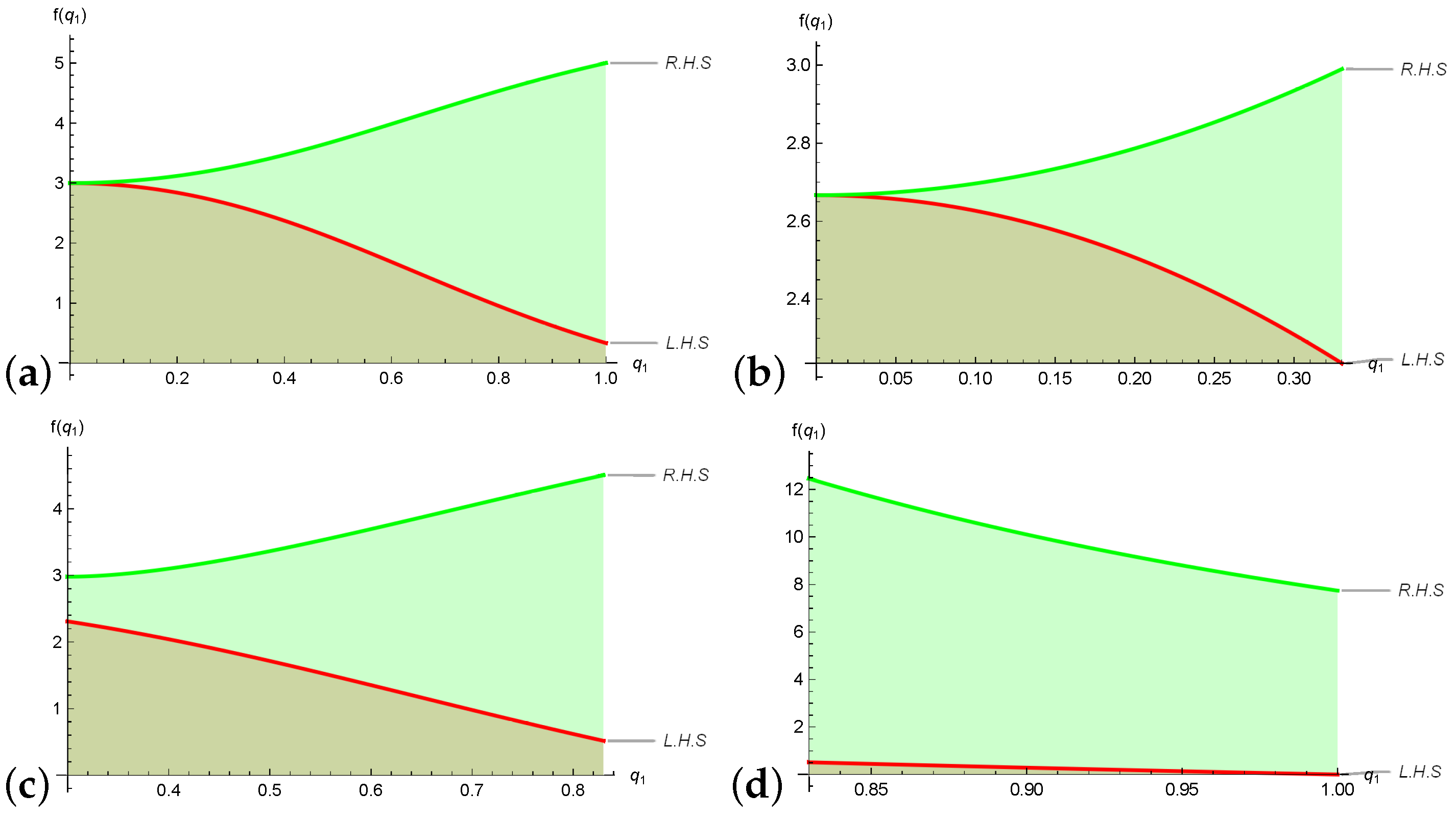
Figure 3a,b demonstrate the accuracy of midpoint and Simpson’s inequalities obtained from Theorem 10. Also, the red and green colors represent the left- and right-sided terms of Theorem 10, respectively.
Theorem 11.
Assume that all the constraints of Lemma 1 are obeyed and | ϱ 1 D q 1 s T | is a Breckner convex mapping with r , p 1 such that 1 p + 1 r = 1 . Then,
λ ( 1 μ ) T ( ϱ 1 ) + λ μ T ( ϱ 2 ) + ( 1 λ ) T ( μ ϱ 2 + ( 1 μ ) ϱ 1 ) q 1 ϱ 2 ϱ 1 ϱ 1 ϱ 2 + ( q 1 1 ) ϱ 1 q 1 T ( β ) 0 d q 1 s β ( ϱ 2 ϱ 1 ) A 1 ( ϑ , λ , μ ) | ϱ 1 D q 1 s T ( ϱ 2 ) | + A 2 ( ϑ , λ , μ ) | ϱ 1 D q 1 s T ( ϱ 1 ) | + A 3 ( ϑ , λ , μ ) | ϱ 1 D q 1 s T ( ϱ 2 ) | + μ 1 ( 1 β ) ϑ | q 1 β + λ μ 1 | | ϱ 1 D q 1 s T ( ϱ 1 ) | 0 d q 1 s β .
Proof. 
From Lemma 1 and Breckner’s convexity, we have
λ ( 1 μ ) T ( ϱ 1 ) + λ μ T ( ϱ 2 ) + ( 1 λ ) T ( μ ϱ 2 + ( 1 μ ) ϱ 1 ) q 1 ϱ 2 ϱ 1 ϱ 1 ϱ 2 + ( q 1 1 ) ϱ 1 q 1 T ( β ) 0 d q 1 s β ( ϱ 2 ϱ 1 ) 0 μ | q 1 β + λ μ λ | | ϱ 1 D q 1 s T ( β ϱ 2 + ( 1 β ) ϱ 1 ) | 0 d q 1 s β + μ 1 | q 1 β + λ μ 1 | | ϱ 1 D q 1 s T ( β ϱ 2 + ( 1 β ) ϱ 1 ) | 0 d q 1 s β ( ϱ 2 ϱ 1 ) 0 μ | q 1 β + λ μ λ | β ϑ | ϱ 1 D q 1 s T ( ϱ 2 ) | + ( 1 β ) ϑ | ϱ 1 D q 1 s T ( ϱ 1 ) | 0 d q 1 s β + μ 1 | q 1 β + λ μ 1 | β ϑ | ϱ 1 D q 1 s T ( ϱ 2 ) | + ( 1 β ) ϑ | ϱ 1 D q 1 s T ( ϱ 1 ) | 0 d q 1 s β = ( ϱ 2 ϱ 1 ) 0 μ β ϑ | q 1 β + λ μ λ | | ϱ 1 D q 1 s T ( ϱ 2 ) | 0 d q 1 s β + 0 μ ( 1 β ) ϑ | q 1 β + λ μ λ | | ϱ 1 D q 1 s T ( ϱ 1 ) | 0 d q 1 s β + μ 1 β ϑ | q 1 β + λ μ 1 | | ϱ 1 D q 1 s T ( ϱ 2 ) | 0 d q 1 s β + μ 1 ( 1 β ) ϑ | q 1 β + λ μ 1 | | ϱ 1 D q 1 s T ( ϱ 1 ) | 0 d q 1 s β .
Finally, by applying Lemma 2, we get the final unified inequality. □
Remark 2.
By taking θ = 1 and lim q 1 , we get the result proven in [34].
Corollary 6.
Inserting ϑ = 1 in Theorem 11, we get the general symmetric quantum bound for convex mappings.
λ ( 1 μ ) T ( ϱ 1 ) + λ μ T ( ϱ 2 ) + ( 1 λ ) T ( μ ϱ 2 + ( 1 μ ) ϱ 1 ) q 1 ϱ 2 ϱ 1 ϱ 1 ϱ 2 + ( q 1 1 ) ϱ 1 q 1 T ( β ) 0 d q 1 s β ( ϱ 2 ϱ 1 ) A 1 ( 1 , λ , μ ) + A 2 ( 1 , λ , μ ) + A 3 ( 1 , λ , μ ) + μ 1 ( 1 β ) | q 1 β + λ μ 1 | | ϱ 1 D q 1 s T ( ϱ 1 ) | 0 d q 1 s β .
Corollary 7.
Inserting λ = μ = 1 2 in Theorem 11, we get the general symmetric quantum bound for convex mappings.
T ( ϱ 1 ) + T ( ϱ 2 ) 4 + 1 2 T ϱ 2 + ϱ 1 2 q 1 ϱ 2 ϱ 1 ϱ 1 ϱ 2 + ( q 1 1 ) ϱ 1 q 1 T ( β ) 0 d q 1 s β ( ϱ 2 ϱ 1 ) A 1 ϑ , 1 2 , 1 2 + A 2 ϑ , 1 2 , 1 2 + A 3 ϑ , 1 2 , 1 2 + μ 1 ( 1 β ) ϑ q 1 β 3 4 | ϱ 1 D q 1 s T ( ϱ 1 ) | 0 d q 1 s β .
Corollary 8.
Inserting λ = μ = 1 3 in Theorem 11, we get the general symmetric quantum bound for convex mappings.
2 T ( ϱ 1 ) + T ( ϱ 2 ) 9 + 2 3 T ϱ 2 + 2 ϱ 1 2 q 1 ϱ 2 ϱ 1 ϱ 1 ϱ 2 + ( q 1 1 ) ϱ 1 q 1 T ( β ) 0 d q 1 s β ( ϱ 2 ϱ 1 ) A 1 ϑ , 1 3 , 1 3 + A 2 ϑ , 1 3 , 1 3 + A 3 ϑ , 1 3 , 1 3 + μ 1 ( 1 β ) ϑ q 1 β 8 9 | ϱ 1 D q 1 s T ( ϱ 1 ) | 0 d q 1 s β .
Example 4.
Let T : [ 0 , 1 ] R be a Breckner convex mapping meeting all the conditions of Theorem 11 and defined as T ( β ) = β 2 . Then, for μ = 1 1 + q 1 2 , and λ = 0 , 1 3 in Theorem 11, we get midpoint-like integral inequality and Simpson-like integral inequality, respectively.
Figure 4a–d demonstrate the accuracy of midpoint and Simpson’s inequalities obtained from Theorem 11. Also, the red and green colors are represent the left- and right-sided terms of Theorem 11, respectively.
Theorem 12.
Assume that all the constraints of Lemma 1 are obeyed and | ϱ 1 D q 1 s T | r is a Breckner convex mapping with r 1 . Then,
λ ( 1 μ ) T ( ϱ 1 ) + λ μ T ( ϱ 2 ) + ( 1 λ ) T ( μ ϱ 2 + ( 1 μ ) ϱ 1 ) q 1 ϱ 2 ϱ 1 ϱ 1 ϱ 2 + ( q 1 1 ) ϱ 1 q 1 T ( β ) 0 d q 1 s β ( ϱ 2 ϱ 1 ) 0 μ q 1 β + λ μ λ 0 d q 1 s β 1 1 r A 1 ( ϑ , λ , μ ) | ϱ 1 D q 1 s T ( ϱ 2 ) | r + A 2 ( ϑ , λ , μ ) | ϱ 1 D q 1 s T ( ϱ 1 ) | r 1 r + μ 1 | q 1 β + λ μ 1 | 0 d q 1 s β 1 r A 3 ( ϑ , λ , μ ) | ϱ 1 D q 1 s T ( ϱ 2 ) | r + μ 1 | q 1 β + λ μ 1 | ( 1 β ) ϑ | ϱ 1 D q 1 s T ( ϱ 1 ) | r 1 1 r .
Proof. 
Through Lemma 1 and Breckner’s convexity, we get
λ ( 1 μ ) T ( ϱ 1 ) + λ μ T ( ϱ 2 ) + ( 1 λ ) T ( μ ϱ 2 + ( 1 μ ) ϱ 1 ) q 1 ϱ 2 ϱ 1 ϱ 1 ϱ 2 + ( q 1 1 ) ϱ 1 q 1 T ( β ) 0 d q 1 s β ( ϱ 2 ϱ 1 ) 0 μ | q 1 β + λ μ λ | | ϱ 1 D q 1 s T ( β ϱ 2 + ( 1 β ) ϱ 1 ) | 0 d q 1 s β + μ 1 | q 1 β + λ μ 1 | | ϱ 1 D q 1 s T ( β ϱ 2 + ( 1 β ) ϱ 1 ) | 0 d q 1 s β 0 μ | q 1 β + λ μ λ | 0 d q 1 s β 1 1 r 0 μ | q 1 β + λ μ λ | | ϱ 1 D q 1 s T ( β ϱ 2 + ( 1 β ) ϱ 1 ) | 0 r d q 1 s β 1 r + μ 1 | q 1 β + λ μ 1 | 0 d q 1 s β 1 1 r 0 μ | q 1 β + λ μ 1 | | ϱ 1 D q 1 s T ( β ϱ 2 + ( 1 β ) ϱ 1 ) | 0 r d q 1 s β 1 r ( ϱ 2 ϱ 1 ) 0 μ | q 1 β + λ μ λ | 0 d q 1 s β 1 1 r 0 1 | q 1 β + λ μ 1 | β ϑ | ϱ 1 D q 1 s T ( ϱ 2 ) | r + ( 1 β ) ϑ | ϱ 1 D q 1 s T ( ϱ 1 ) | r 0 d q 1 s β 1 r + μ 1 | q 1 β + λ μ 1 | 0 d q 1 s β 1 1 r 0 μ β ϑ | ϱ 1 D q 1 s T ( ϱ 2 ) | r + ( 1 β ) ϑ | ϱ 1 D q 1 s T ( ϱ 1 ) | r 0 d q 1 s β 1 r = ( ϱ 2 ϱ 1 ) 0 μ | q 1 β + λ μ λ | 0 d q 1 s β 1 1 r 0 μ β ϑ | q 1 β + λ μ λ | | ϱ 1 D q 1 s T ( ϱ 2 ) | 0 r d q 1 s β + 0 μ ( 1 β ) ϑ | q 1 β + λ μ λ | | ϱ 1 D q 1 s T ( ϱ 1 ) | 0 r d q 1 s β 1 r + μ 1 | q 1 β + λ μ 1 | 0 d q 1 s β 1 1 r μ 1 β ϑ | q 1 β + λ μ 1 | | ϱ 1 D q 1 s T ( ϱ 2 ) | 0 r d q 1 s β + μ 1 ( 1 β ) ϑ | q 1 β + λ μ 1 | | ϱ 1 D q 1 s T ( ϱ 1 ) | 0 r d q 1 s β 1 r .
Some simple computations through Lemma 2 and Lemma 3 yield the desired bound. □
It is important to note that for q = 1 , we recapture Theorem 11.
Remark 3.
By taking θ = 1 and lim q 1 , we get the result proven in [34].
Corollary 9.
Inserting ϑ = 1 in Theorem 12, we get the general error inequality for symmetric quantum differentiable convex mappings.
λ ( 1 μ ) T ( ϱ 1 ) + λ μ T ( ϱ 2 ) + ( 1 λ ) T ( μ ϱ 2 + ( 1 μ ) ϱ 1 ) q 1 ϱ 2 ϱ 1 ϱ 1 ϱ 2 + ( q 1 1 ) ϱ 1 q 1 T ( β ) 0 d q 1 s β ( ϱ 2 ϱ 1 ) 0 μ q 1 β + λ μ λ 0 d q 1 s β 1 1 r A 1 1 , λ , μ + A 2 1 , λ , μ 1 r + μ 1 | q 1 β + λ μ 1 | 0 r d q 1 s β 1 1 r A 1 1 , λ , μ + μ 1 | q 1 β + λ μ 1 | ( 1 β ) | ϱ 1 D q 1 s T ( ϱ 1 ) | r 1 r .
Example 5.
Let T : [ 0 , 1 ] R be a Breckner convex mapping meeting all the conditions of Theorem 12 and defined as T ( β ) = β 2 with r = 2 . Then, for μ = 1 1 + q 1 2 , choosing λ = 0 , 1 3 in Theorem 12, we get midpoint-like integral inequality and Simpson-like integral inequality, respectively.
Figure 5a–d demonstrate the accuracy of midpoint and Simpson’s inequalities obtained from Theorem 12. Also, the red and green colors are represent the left and right-sided terms of Theorem 12, respectively.

3. Applications

Now, we generate a few inequalities between binary means and composite error bounds corresponding to symmetric quantum integrals. First, we recall a few important means.
  • The weighted arithmetic mean is as follows:
    A w ( ϱ 1 , ϱ 2 ; w 1 , w 2 ) = w 1 ϱ 1 + w 2 ϱ 2 w 1 + w 2 ,
  • The generalized r-log-mean is as follows:
    L r ( ϱ 1 , ϱ 2 ) = ϱ 2 r + 1 ϱ 1 r + 1 ( r + 1 ) ( ϱ 2 ϱ 1 ) 1 r ; r { 1 , 0 } .

3.1. Application to Means

Proposition 1.
Assume that all the assumptions of Theorem 8 are correct, we have the following inequality.
2 ϑ A δ + 1 ( ϱ 1 , ϱ 2 ) δ + 1 2 L δ δ + 1 ( ϱ 1 , ϱ 2 ) δ + 1 4 A ( ϱ 1 δ + 1 , ϱ 2 δ + 1 ) ( ϑ + 1 ) ( δ + 1 ) .
Proof. 
Applying T ( β ) = β δ + 1 δ + 1 , δ 1 on Theorem 8 and taking lim q 1 1 m, we get the required result. □
Proposition 2.
Assuming that all the assumptions of Theorem 10 are correct, we have the following inequality.
λ A w ( ϱ 1 δ + 1 , ϱ 2 δ + 1 ; u , 1 u ) δ + 1 + ( 1 λ ) A w δ + 1 ( ϱ 1 , ϱ 2 ; u , 1 u ) δ + 1 L δ δ + 1 ( ϱ 1 , ϱ 2 ) δ + 1 ( ϱ 2 ϱ 1 ) 0 μ | q 1 β + λ μ 1 | 0 p d q 1 s β 1 p μ ϑ + 1 | ϱ 2 δ | r ϑ + 1 ( 1 μ ) ϑ + 1 | ϱ 1 δ | r ϑ + 1 + | ϱ 1 δ | r ϑ + 1 1 r + μ 1 | q 1 β + λ μ 1 | 0 p d q 1 s β 1 p | ϱ 2 δ | r ϑ + 1 μ ϑ + 1 | ϱ 2 δ | r ϑ + 1 + ( 1 μ ) ϑ + 1 | ϱ 1 δ | r ϑ + 1 1 r .
Proof. 
Applying T ( β ) = β δ + 1 δ + 1 , δ 2 to Theorem 10 and taking lim q 1 1 , we get the required result. □

3.2. Unified Symmetric Quantum Error Boundaries of Composite-Type Scheme

Suppose that the partition P of [ ϱ 1 , ϱ 2 ] is given as ϱ 1 = ϕ 0 < ϕ 1 . . . . . . < ϕ δ = ϱ 2 . The generalized parametric family of rule is given as
ϱ 1 ϱ 2 + ( q 1 1 ) ϱ 1 q 1 T ( β ) 0 d q 1 s β = T δ ( T , ϕ , q 1 ) + R δ ( T , ϕ , q 1 ) ,
where
T δ ( T , ϕ , q 1 ) = ( ϕ i + 1 ϕ i ) q 1 λ T ( ϕ i ) + λ μ ( T ( ϕ i + 1 ) T ( ϕ i ) ) + ( 1 λ ) T ( μ ϕ i + 1 + ( 1 μ ) ϕ i ) .
and R δ ( T , ϕ , q 1 ) represents the error of the above discussed rule.
Proposition 3.
Undertaking the conditions of Theorem 10, we get the following bound
| R δ ( T , ϕ , q 1 ) | i = o δ 1 ( ϕ i + 1 ϕ i ) 2 q 1 0 μ | q 1 β + λ μ λ | 0 p d q 1 s β 1 p 0 μ β ϑ | ϕ i D q 1 s T ( ϕ i + 1 ) | 0 r d q 1 s β + 0 μ ( 1 β ) ϑ | ϕ i D q 1 s T ( ϕ i ) | 0 r d q 1 s β 1 r + μ 1 | q 1 β + λ μ 1 | 0 p d q 1 s β 1 p μ 1 β ϑ | ϕ i D q 1 s T ( ϕ i + 1 ) | 0 r d q 1 s β + μ 1 ( 1 β ) ϑ | ϱ 1 D q 1 s T ( ϕ i ) | 0 r d q 1 s β 1 r .
Proof. 
By applying Theorem 10 on [ ϕ i , ϕ i + 1 ] and summing from i = 0 to i = δ 1 , we acquire the final inequality. □
Proposition 4.
Undertaking the conditions of Theorem 11, we get the following bound
| R δ ( T , ϕ , q 1 ) | i = o δ 1 ( ϕ i + 1 ϕ i ) 2 q 1 0 μ β ϑ | q 1 β + λ μ λ | | ϕ i D q 1 s T ( ϕ i + 1 ) | 0 d q 1 s β + 0 μ ( 1 β ) ϑ | q 1 β + λ μ λ | | ϕ i D q 1 s T ( ϕ i ) | 0 d q 1 s β + μ 1 β ϑ | | q 1 β + λ μ 1 | ϕ i D q 1 s T ( ϕ i + 1 ) | 0 d q 1 s β + μ 1 ( 1 β ) ϑ | q 1 β + λ μ 1 | | ϕ i D q 1 s T ( ϕ i ) | 0 d q 1 s β .
Proof. 
By applying Theorem 11 to [ ϕ i , ϕ i + 1 ] and summing from i = 0 to i = δ 1 , we acquire the final inequality. □

4. Concluding Remarks and Future Directions

Quantum calculus generalizes classical concepts and is very useful for discussing discontinuous mappings. Researchers have expanded the quantum calculus in diverse directions, including inequalities, optimization, calculus of variation, and special mappings. The symmetric operators are widely employed to examine the differentiability of several non-differentiable mappings. Recently, authors have focused on the symmetric quantum calculus to refine the classical counterparts of inequalities, special mappings, and impulsive difference equations. In this manuscript, we have developed some new refinements of Hermite–Hadamard kinds of inequalities pertaining to Breckner’s convexity. Our results are generic in nature; by the variation of parameters, a blend of new inequalities can be obtained. Also, our results provide the bounds of symmetric quantum integrals of various non-convex mappings. Furthermore, some theoretical applications have been presented. By using the developed parametric bounds, several existing new iterative schemes of cubic order of convergence can be obtained.
In the future, we will try to expand the results for symmetric quantum fractional operators. Another important problem is the development of H-H-type inequalities associated with fuzzy symmetric fractional operators. To the best of our knowledge, the fuzzy symmetric quantum and their fractional variants are not introduced in the literature. By using the strong and generalized classes of convexity and newly developed identity, numerous new bounds can be developed.

Author Contributions

Conceptualization, M.Z.J., N.N. and M.U.A.; methodology, M.Z.J., N.N., M.U.A., Y.W. and O.M.A.; software, M.Z.J. and N.N.; validation, M.Z.J., N.N., M.U.A., Y.W. and O.M.A.; formal analysis, M.Z.J., N.N., M.U.A., Y.W. and O.M.A.; investigation, M.Z.J., N.N., M.U.A., Y.W. and O.M.A.; writing—original draft preparation, M.Z.J. and N.N.; writing—review and editing, M.Z.J., N.N., M.U.A., Y.W. and O.M.A.; visualization, M.Z.J., N.N., M.U.A., Y.W. and O.M.A.; supervision, M.U.A. All authors have read and agreed to the published version of the manuscript.

Funding

This research was funded by TAIF University, TAIF, Saudi Arabia, Project No. (TU-DSPP-2024-258).

Data Availability Statement

The original contributions presented in this study are included in the article, and further inquiries can be directed to the corresponding author.

Acknowledgments

The authors are thankful to the National Natural Science Foundation of China for funding this project under Grant 12171435. The authors extend their appreciation to TAIF University, Saudi Arabia, for supporting this work through project number (TU-DSPP-2024-258). The authors are grateful to the editor and the anonymous reviewers for their valuable comments and suggestions.

Conflicts of Interest

The authors declare no conflicts of interest.

References

  1. Roberts, A.W.; Varberg, D.E. Convex Functions, 1st ed.; Academic Press: New York, NY, USA, 1974; Volume 57. [Google Scholar]
  2. Dragomir, S.S.; Fitzpatrick, S. The Jensen inequality for s-Breckner convex functions in linear spaces. Demonstr. Math. 2000, 33, 43–50. [Google Scholar] [CrossRef]
  3. Beckenbach, E.F. Convex functions. Bull. Am. Math. Soc. 1948, 54, 439–460. [Google Scholar] [CrossRef]
  4. Niculescu, C.; Persson, L.E. Convex Functions and Their Applications; Springer: New York, NY, USA, 2006; Volume 23. [Google Scholar]
  5. Dragomir, S.S.; Fitzpatrick, S. The Hadamard inequalities for s-convex functions in the second sense. Demonstr. Math. 1999, 32, 687–696. [Google Scholar] [CrossRef]
  6. Tseng, K.L.; Hwang, S.R.; Dragomir, S.S. On some new inequalities of Hermite-Hadamard Fejér type involving convex functions. Demonstr. Math. 2007, 40, 51–64. [Google Scholar] [CrossRef]
  7. Dragomir, S.S.; Pearce, C. Selected topics on Hermite–Hadamard inequalities and applications. Sci. Direct Work. Pap. 2003, S1574-0358-04. Available online: https://ssrn.com/abstract=3158351 (accessed on 12 April 2018).
  8. Butt, S.I.; Pecaric, J. Generalized Hermite–Hadamard’s inequality. Proc. A Razmadze Math. Inst. 2013, 163, 9. [Google Scholar]
  9. Srivastava, H.M.; Mehrez, S.; Sitnik, S.M. Hermite–Hadamard-type integral inequalities for convex functions and their applications. Mathematics 2022, 10, 3127. [Google Scholar] [CrossRef]
  10. Alomari, M. Several Inequalities of Hermite–Hadamard, Ostrowski and Simpson Type for s-Convex, Quasi-Convex and r-Convex Mappings and Applications. Ph.D. Thesis, Universiti Kebangsaan Malaysia, Bangi, Malaysia, 2008. [Google Scholar]
  11. Davis, P.J.; Rabinowitz, P. Methods of Numerical Integration; Academic Press: New York, NY, USA, 1975. [Google Scholar]
  12. Alomari, M.; Darus, M.; Dragomir, S.S. New inequalities of Simpson’s type for s-convex functions with applications. Res. Rep. Coll. 2009, 12, 4. [Google Scholar]
  13. Tariboon, J.; Ntouyas, S.K. Quantum calculus on finite intervals and applications to impulsive difference equations. Adv. Differ. Equ. 2013, 2013, 282. [Google Scholar] [CrossRef]
  14. Alp, N.; Sarıkaya, M.Z.; Kunt, M.; İşcan, İ. q-Hermite–Hadamard inequalities and quantum estimates for midpoint type inequalities via convex and quasi-convex functions. J. King Saud Univ. Sci. 2018, 30, 193–203. [Google Scholar] [CrossRef]
  15. Kunt, M.; Baidar, A.W.; Sanli, Z. Some quantum integral inequalities based on left-right quantum integrals. Turk. J. Sci. Technol. 2022, 17, 343–356. [Google Scholar] [CrossRef]
  16. Da Cruz, A.M.C.B. Symmetric Quantum Calculus. Ph.D. Thesis, Universidade de Aveiro, Aveiro, Portugal, 2012. [Google Scholar]
  17. Bilal, M.; Iqbal, A.; Rastogi, S. Quantum symmetric analogues of various integral inequalities over finite intervals. J. Math. Inequal. 2023, 17, 615–627. [Google Scholar] [CrossRef]
  18. Vivas-Cortez, M.; Javed, M.Z.; Awan, M.U.; Dragomir, S.S.; Zidan, A.M. Properties and applications of symmetric quantum calculus. Fractal Fract. 2024, 8, 107. [Google Scholar] [CrossRef]
  19. Sudsutad, W.; Ntouyas, S.K.; Tariboon, J. Quantum integral inequalities for convex functions. J. Math. Inequal. 2015, 9, 781–793. [Google Scholar] [CrossRef]
  20. Jhanthanam, S.; Tariboon, J.; Ntouyas, S.K.; Nonlaopon, K. On q-Hermite–Hadamard inequalities for differentiable convex functions. Mathematics 2019, 7, 632. [Google Scholar] [CrossRef]
  21. Kunt, M.; Kashuri, A.; Du, T.S.; Baidar, A.W. Quantum Montgomery identity and quantum estimates of Ostrowski type inequalities. AIMS Math. 2020, 5, 5439–5457. [Google Scholar] [CrossRef]
  22. Bin-Mohsin, B.; Javed, M.Z.; Awan, M.U.; Khan, A.G.; Cesarano, C.; Noor, M.A. Exploration of quantum Milne–Mercer-type inequalities with applications. Symmetry 2023, 15, 1096. [Google Scholar] [CrossRef]
  23. Ali, M.A.; Budak, H.; Fečkan, M.; Khan, S. A new version of q-Hermite–Hadamard’s midpoint and trapezoid type inequalities for convex functions. Math. Slovaca 2023, 73, 369–386. [Google Scholar] [CrossRef]
  24. Khan, M.A.; Mohammad, N.; Nwaeze, E.R.; Chu, Y.M. Quantum Hermite–Hadamard inequality by means of a Green function. Adv. Differ. Equ. 2020, 2020, 99. [Google Scholar] [CrossRef]
  25. Saleh, W.; Meftah, B.; Lakhdari, A. Quantum dual Simpson type inequalities for q-differentiable convex functions. Int. J. Nonlinear Anal. Appl. 2023, 14, 63–76. [Google Scholar]
  26. Du, T.S.; Luo, C.Y.; Yu, B. Certain quantum estimates on the parameterized integral inequalities and their applications. J. Math. Inequal. 2021, 15, 201–228. [Google Scholar] [CrossRef]
  27. Bin-Mohsin, B.; Javed, M.Z.; Awan, M.U.; Budak, H.; Kara, H.; Noor, M.A. Quantum integral inequalities in the setting of majorization theory and applications. Symmetry 2022, 14, 1925. [Google Scholar] [CrossRef]
  28. Budak, H.; Ali, M.A.; Tarhanaci, M. Some new quantum Hermite–Hadamard-like inequalities for coordinated convex functions. J. Optim. Theory Appl. 2020, 186, 899–910. [Google Scholar] [CrossRef]
  29. Nosheen, A.; Ijaz, S.; Khan, K.A.; Awan, K.M.; Albahar, M.A.; Thanoon, M. Some q-symmetric integral inequalities involving s-convex functions. Symmetry 2023, 15, 1169. [Google Scholar] [CrossRef]
  30. Butt, S.I.; Aftab, M.N.; Seol, Y. Symmetric quantum inequalities on finite rectangular plane. Mathematics 2024, 12, 1517. [Google Scholar] [CrossRef]
  31. Liu, Q.; Javed, M.Z.; Awan, M.U.; Ciurdariu, L.; Alkahtani, B.S. Hermite–Hadamard’s like inequalities via symmetric quantum calculus. Ain Shams Eng. J. 2025, 16, 103372. [Google Scholar] [CrossRef]
  32. Nosheen, A.; Ijaz, S.; Khan, K.A.; Awan, K.M.; Budak, H. Quantum symmetric integral inequalities for convex functions. Math. Methods Appl. Sci. 2024, 47, 14878–14895. [Google Scholar] [CrossRef]
  33. Wang, Y.; Javed, M.Z.; Awan, M.U.; Bin-Mohsin, B.; Meftah, B.; Treanta, S. Symmetric quantum calculus in interval valued framework: Operators and applications. AIMS Math. 2024, 9, 27664–27686. [Google Scholar] [CrossRef]
  34. İşcan, İ. A new generalization of some integral inequalities and their applications. Int. J. Eng. 2013, 3, 8269. [Google Scholar]
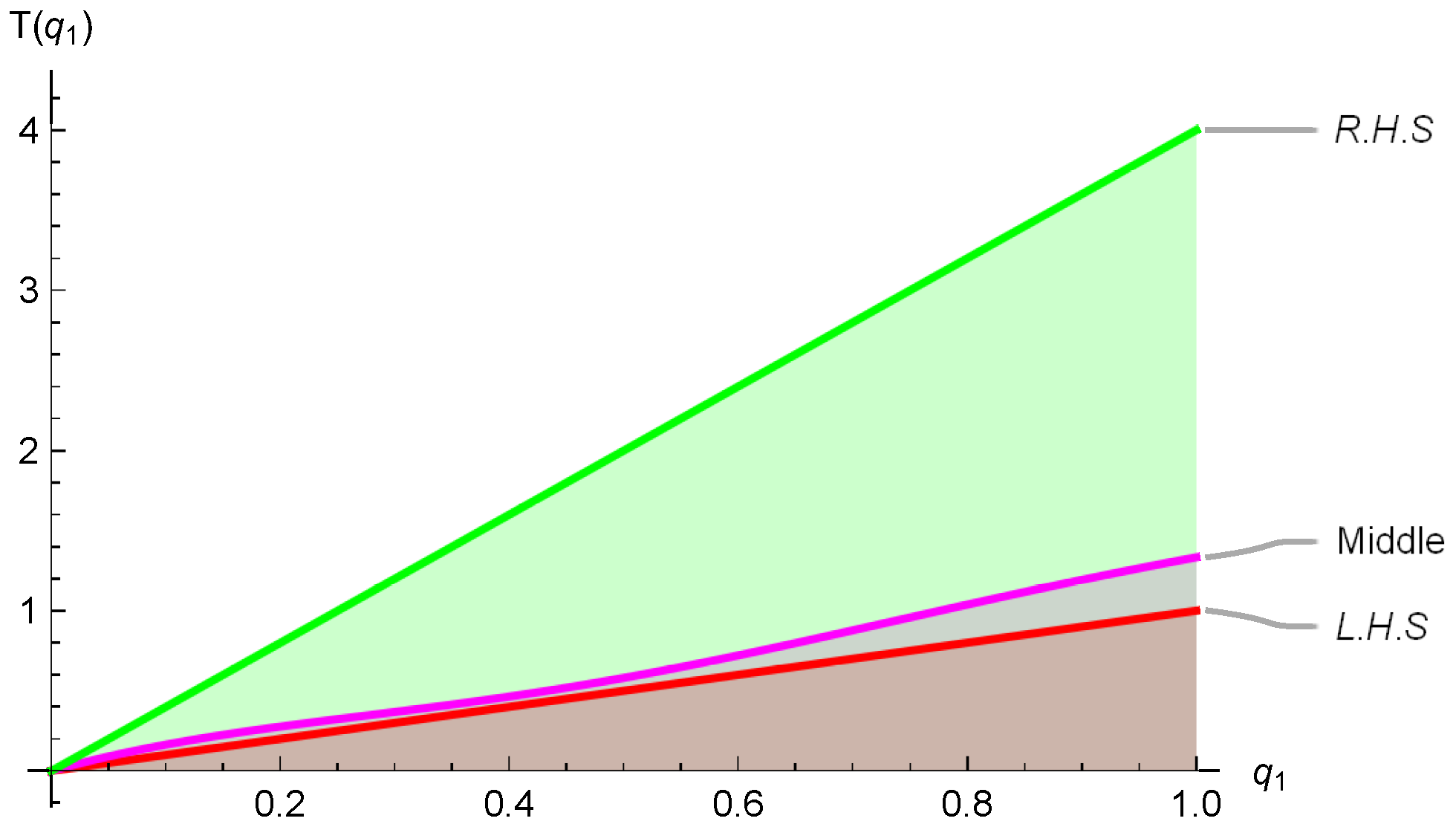
Figure 1. Visual analysis of Theorem 8.
Mathematics 13 02910 g001
Figure 2. Visual analysis of Theorem 9.
Mathematics 13 02910 g002
Figure 3. (a) Visual analysis of Theorem 10 for (a) μ = 1 1 + q 1 2 , and λ = 0 ; (b) μ = 1 1 + q 1 2 , and λ = 1 3 .
Mathematics 13 02910 g003
Figure 4. Visual analysis of Theorem 11 for (a) μ = 1 1 + q 1 2 , and λ = 0 ; (b) μ = 1 1 + q 1 2 , λ = 1 3 , and q 1 = [ 0 , 0.33 ) ; (c) μ = 1 1 + q 1 2 , λ = 1 3 , and q 1 = [ 0.33 , 0.833 ) ; (d) μ = 1 1 + q 1 2 , λ = 1 3 , and q 1 = [ 0.83 , 1 ) .
Mathematics 13 02910 g004
Figure 5. Visual analysis of Theorem 12 for (a) μ = 1 1 + q 1 2 , and λ = 0 ; (b) μ = 1 1 + q 1 2 , λ = 1 3 , and q 1 = [ 0 , 0.33 ) . (c) μ = 1 1 + q 1 2 , λ = 1 3 , and q 1 = [ 0.33 , 0.83 ) ; (d) μ = 1 1 + q 1 2 , λ = 1 3 , and q 1 = [ 0.83 , 1 ) .
Mathematics 13 02910 g005aMathematics 13 02910 g005b
Disclaimer/Publisher’s Note: The statements, opinions and data contained in all publications are solely those of the individual author(s) and contributor(s) and not of MDPI and/or the editor(s). MDPI and/or the editor(s) disclaim responsibility for any injury to people or property resulting from any ideas, methods, instructions or products referred to in the content.