Forecasting Upper Bounds for Daily New COVID-19 Infections Using Tolerance Limits

Abstract

Coronavirus disease 2019 (COVID-19), caused by severe acute respiratory syndrome coronavirus 2 (SARS-CoV-2), was first identified in Wuhan, China, in December 2019. Since then, it has evolved into a global pandemic. Forecasting the number of COVID-19 cases is a crucial task that can greatly aid management decisions. Numerous methods have been proposed in the literature to forecast COVID-19 case numbers; however, most do not yield highly accurate results. Rather than focusing solely on predicting exact case numbers, providing robust upper bounds may offer a more practical approach to support effective decision-making and resource preparedness. This study proposes the use of tolerance interval methods to construct upper bounds for daily new COVID-19 case numbers. The tolerance limits derived from the normal, Poisson, and negative binomial distributions are compared. These methods rely either on historical data alone or on a combination of historical data and auxiliary data from other regions. The results demonstrate that the proposed methods can generate informative upper bounds for COVID-19 case counts, offering a valuable alternative to traditional forecasting models that emphasize exact number estimation. This approach can improve pandemic preparedness through better equipment planning, resource allocation, and timely response strategies.

1. Introduction

Coronavirus disease 2019 (COVID-19) is a disease caused by the severe acute respiratory syndrome coronavirus 2 (SARS-CoV-2), which led to a worldwide pandemic [1]. In the early 2000s, there was also a pandemic of an acute respiratory syndrome known as Severe Acute Respiratory Syndrome (SARS), caused by SARS-CoV-1 [2,3]. The impact of SARS is comparatively lower when compared to that of COVID-19. SARS caused a significant outbreak primarily in Asia [4], whereas COVID-19 led to distinct waves in various regions, resulting in a much more profound global impact.

The COVID-19 pandemic began in China and subsequently spread to Europe and the United States (USA) [5]. The pandemic resulted in multiple waves of cases and deaths worldwide [6]. After the initial onset, the major waves of COVID-19 infections were primarily attributable to the emergence of concerning variants. When a new variant emerges and becomes predominant, it can contribute to another wave of the COVID-19 pandemic. Over time, SARS-CoV-2 has undergone several mutations, resulting in different variants such as Alpha, Beta, Gamma, and Delta [7]. Some of these variants were the principal culprits behind these waves [8]. When a new strain emerges, waves can occur in different areas at different times. For example, during the initial COVID-19 pandemic, China experienced an outbreak earlier than Europe and the USA [5]. The forecasting of COVID-19 case numbers is an important issue in each pandemic wave that can contribute to effective pandemic control and healthcare resource management.

Numerous approaches have been suggested in the literature for predicting COVID-19 case numbers (see the Section 4), but most fall short of delivering highly precise results. Offering reliable upper bounds for the count of COVID-19 cases, rather than predicting the exact number, could be a more pragmatic strategy. This alternative approach can aid in making effective decisions for managing COVID-19 and ensuring appropriate resource readiness. If an upper bound can be predicted for each week in such a way that, for example, 90% of the daily new COVID-19 case numbers are below this upper bound with a 95% confidence level, then this upper bound can provide valuable information to facilitate early management preparations. It is unnecessary to set an upper bound requiring 100% of numbers to be below it because it may lead to an overly conservative bound demanding excessive resource allocation. In this study, tolerance interval methods based solely on historical data or on both historical data and auxiliary data from another region are proposed to establish upper tolerance bounds for the daily new COVID-19 case numbers.

In statistical estimation, when the target is a parameter, which is a single point, a confidence interval can be used to estimate it. However, in some situations, the interest lies in estimating a range rather than a point. In such cases, when the target is an interval, a tolerance interval is the appropriate choice [9]. For example, a confidence interval is used to estimate a population parameter (e.g., the mean), whereas a tolerance interval is used to estimate a range that contains a specified proportion of the population. In this study, the term “population” refers to the daily number of newly confirmed cases. Since the primary concern is a high daily number of newly confirmed cases, rather than a low number, an upper tolerance limit is considered instead of a two-sided tolerance interval. The upper tolerance limits are constructed so that, with 95% confidence, they cover 99% of the population; in other words, 99% of the daily new counts are expected to fall below these limits. The study emphasizes forecasting an upper bound for daily confirmed case counts, rather than forecasting the counts themselves.

When predicting the upper bound for COVID-19 case numbers, an important consideration is the appropriate timeframe for using historical data, such as 7 or 14 days. This study reviews the relevant literature and considers both 7-day and 14-day timeframes. In a machine learning algorithm study for analyzing COVID-19 data in six locations within Nigeria, all models required data for the past 7 days to make optimal predictions in Kebbi State [10]. The forecasting of future COVID-19 cases for the next 7 and 14 days, focusing on highly affected countries such as India, the USA, the UK, Russia, Brazil, Germany, France, Italy, Turkey, and Colombia, was examined [11]. The performance of deep learning models for forecasting the COVID-19 cases in three countries, namely, Brazil, India, and Russia, was compared, and the best-performing model was selected to forecast cases for the future 7 days [12]. These studies revealed that using the past 7- or 14-day data could be a good choice for forecasting COVID-19 case numbers in the next 7 or 14 days. As a result, the two situations of using the past 7 or 14 days are considered in this study.

The upper tolerance limits based on the normal, Poisson, and negative binomial models are considered in this study, using the past 7 or 14 days of data to predict the upper bounds for the next 7 or 14 days. The datasets analyzed are from two countries: the United States (USA) and the United Kingdom (UK). The number of daily new COVID-19 cases is count data, so discrete distributions can be used for modeling. However, the Poisson distribution does not fit these two datasets well, while the negative binomial distribution performs better in fitting them. Previous research has shown that a mixture normal distribution performs well in monitoring COVID-19 data [13]. Therefore, the normal distribution is also considered in this study. Since a normal distribution can be viewed as a mixture normal distribution with one component, we do not consider higher-component mixture normal distributions, as the available 7- or 14-day data segments are too small to fit them reliably. The results show that the upper tolerance limits derived from the normal distribution outperform those obtained from the Poisson and negative binomial distributions.

In addition, to improve the prediction result, the historical data from other regions might be used as auxiliary data to aid in COVID-19 case number prediction. The inferences based on auxiliary data have been used as important tools for analyzing data in a variety of applications, including the analysis of COVID-19 data [14,15]. The utility of auxiliary indicators has been shown to improve the predictive accuracy of autoregressive models in COVID-19 forecasting [15]. Auxiliary indicators of COVID activity in the USA, measured at the county level and updated daily, were provided in open-access databases, and these indicators could provide alternate views on pandemic activity [16]. These previous studies have revealed that incorporating useful auxiliary data could enhance COVID-19 forecasting. Therefore, in addition to using the conventional tolerance bound, this study derives a form of upper tolerance bound incorporating auxiliary data.

The novelty of this study lies in (i) proposing the use of upper tolerance limits as upper bounds for forecasting COVID-19 case numbers and (ii) incorporating data from other regions to improve forecasting accuracy. The results show that both approaches contribute to COVID-19 forecasting, with the incorporation of auxiliary data further enhancing accuracy.

2. Materials and Methods

2.1. Concept and Upper Tolerance Bound for the Normal Distribution

Tolerance intervals have extensive utilization across diverse domains, encompassing manufacturing, engineering, clinical research, and the pharmaceutical industries. The tolerance intervals for various distributions have been established [17]. There are usually two typical types of tolerance intervals, $\beta -\mathrm{c}\mathrm{o}\mathrm{n}\mathrm{t}\mathrm{e}\mathrm{n}\mathrm{t}$ tolerance interval and $\beta -\mathrm{e}\mathrm{x}\mathrm{p}\mathrm{e}\mathrm{c}\mathrm{t}\mathrm{a}\mathrm{t}\mathrm{i}\mathrm{o}\mathrm{n}$ tolerance interval, where $\beta$ denotes a proportion between 0 and 1 [18,19]. The $\beta -$ content tolerance interval is used in this study.

An interval $(L\left(X\right), U\left(X\right))$ is said to be a two-sided $\beta -$ content, $1-\alpha$ confidence level tolerance interval, denoted by $(\beta ,1-\alpha )$ tolerance interval, for a distribution $F$ if

$$P\left\{\left[F\left(U\left(X\right)\right)-F\left(L\left(X\right)\right)\ge \beta \right]\right\}=1-\alpha$$

where $X$ is a random variable with a distribution function $F$. One-sided tolerance bounds can be defined similarly. A tolerance bound $U\left(X\right)$ is said to be an upper $(\beta ,1-\alpha )$ tolerance bound for $F$ if

$$P\left\{F\left(U\left(X\right)\right)\ge \beta \right\}=1-\alpha$$

(1)

When predicting COVID-19 cases, the primary concern is the high number of cases, not the low number. Consequently, only the upper tolerance bound needs to be considered in this study. For the normal distribution, the exact form of an upper (β, 1 − α) tolerance bound based on a sample with sample size $n$ has the form

$$UTL=\overline{x}+k{s}_x$$

(2)

where $\overline{x}$ and $s_x$ are the sample mean and sample standard deviation. The formula of the factor $k$ is

$$k={\displaystyle \frac{z_{\beta }+\sqrt{z_{\beta }^2-ab}}{a}}$$

(3)

where

$$a=1-{\displaystyle \frac{z_{1-\alpha }^2}{2(n-1)}}$$

$$b=z_{\beta }^2-{\displaystyle \frac{z_{1-\alpha }^2}{n}}$$

and ${\mathrm{z}}_{\mathrm{r}}$ denotes the $r\mathrm{t}\mathrm{h}$ quantile of the standard normal distribution [20,21].

When auxiliary data $Y$ from another region are used to predict the COVID-19 case numbers of a specific region, the data from the two regions can be modeled by a bivariate normal distribution. The density function of the bivariate normal distribution is

$$f_{XY}(x,y)={\displaystyle \frac{1}{2\pi {\sigma }_X{\sigma }_Y\sqrt{1-{\rho }^2}}}{e}^{-{\displaystyle \frac{1}{2\left(1-{\rho }^2\right)}}\left[{\left({\displaystyle \frac{x-{\mu }_X}{{\sigma }_X}}\right)}^2+{\left({\displaystyle \frac{y-{\mu }_Y}{{\sigma }_Y}}\right)}^2-2\rho {\displaystyle \frac{\left(x-{\mu }_X\right)\left(y-{\mu }_Y\right)}{{\sigma }_X{\sigma }_Y}}\right]}$$

where ${\mu }_X$ and ${\mu }_Y$ denote the means of $\mathrm{X}$ and $Y$, respectively, ${\sigma }_X$ and ${ \sigma }_Y$ denote the standard deviations of $\mathrm{X}$ and $Y$, respectively, and $\rho$ denotes the correlation coefficient between $\mathrm{X}$ and $Y$.

The conditional density function $f\left(x\right|y)$ of $X$ given $Y=y$ is a normal distribution with the mean and variance as follows:

$$E[X\mid Y=y]={\mu }_X+\rho {\displaystyle \frac{{\sigma }_X}{{\sigma }_Y}}(y-{\mu }_Y)$$

and

$$Var(X\mid Y=y)=\left(1-{\rho }^2\right){\sigma }_X^2$$

Thus, since the conditional distribution is normal, according to (2), an upper tolerance bound based on the conditional distribution is

$$\widetilde{UTL}={\widehat{\mu }}_X+\widehat{\rho }{\displaystyle \frac{{\widehat{\sigma }}_X}{{\widehat{\sigma }}_Y}}\left(y-{\widehat{\mu }}_Y\right)+k{\widehat{\sigma }}_X\sqrt{1-{\widehat{\rho }}^2}$$

(4)

where ${\widehat{\mu }}_x=\overline{x},{\widehat{\sigma }}_x=s_x,{\widehat{\mu }}_y=\overline{y,}$ and ${\widehat{\sigma }}_y=s_y$ denote the sample means and standard deviations of the observed historical data of $X$ and $Y$, and $\widehat{\rho }$ denotes the sample correlation coefficient of the historical data of $X$ and $Y$. However, since $-1<\rho <1$, this bound

$${UTL}^{*}=\underset{-1<\rho <1}{\mathit{max}}\left\{{\widehat{\mu }}_X+\rho {\displaystyle \frac{{\widehat{\sigma }}_X}{{\widehat{\sigma }}_Y}}\left(y-{\widehat{\mu }}_Y\right)+k{\widehat{\sigma }}_X\sqrt{1-{\rho }^2} \right\},$$

(5)

by selecting a $\rho$ such that (4) attaining a maximum in $\rho$ can be considered as a better upper tolerance bound of $X$ given $Y=y.$ However, since (5) is modified mainly based on the auxiliary data $Y$, and considering the importance of the method based on historical data of $X$, it is not advisable to rely solely on Equation (5) as an upper tolerance bound. Therefore, a modified upper tolerance bound

$${UTL}^{**}=\mathit{max}\left(UTL,{UTL}^{*}\right)$$

(6)

is proposed, which can take into account both historical data and auxiliary data. The details of calculating this upper bound are provided in Procedure 1 in Section 3.3.

To find (5), we have the following theorem:

Theorem 1.

Let

$${\rho }_{MAX}=\left\{\begin{array}{c}{\displaystyle \frac{y-{\widehat{\mu }}_Y}{\sqrt{(y-{\widehat{\mu }}_Y{)}^2+k^2{{\widehat{\sigma }}_Y}^2}}} when y\ge {\widehat{\mu }}_Y\\ {\displaystyle \frac{{\widehat{\mu }}_Y-y}{\sqrt{(y-{\widehat{\mu }}_Y{)}^2+k^2{{\widehat{\sigma }}_Y}^2}}} when y<{\widehat{\mu }}_Y\end{array}\right.$$

(7)

If the denominator of (7) is zero, then${ \rho }_{MAX }$is set to zero. Then

$${UTL}^{*}={\widehat{\mu }}_X+{\rho }_{MAX}{\displaystyle \frac{{\widehat{\sigma }}_X}{{\widehat{\sigma }}_Y}}\left(y-{\widehat{\mu }}_Y\right)+k{\widehat{\sigma }}_X\sqrt{1-{{\rho }_{MAX}}^2}$$

(8)

The proof of Theorem 1 is provided in Appendix A.

2.2. Poisson Distribution

In addition to utilizing the normal distribution, the Poisson distribution can be considered to fit the daily number of newly confirmed cases, given that it is a discrete variable. The tolerance intervals for the Poisson distribution have been established [9,22,23]. The two tolerance intervals proposed by Cai and Wang (2009) [23], called the first-order and second-order probability-matching (β, 1 − α) upper tolerance bounds, have the forms

$$X+a_1+b_1\sqrt{X}$$

(9)

and

$$X+a_1+b_1\sqrt{X+c_1}$$

(10)

respectively, where

$$a_1={\displaystyle \frac{1}{6}}\left(z_{1-\alpha }+z_{\beta }\right)\left(2z_{1-\alpha }+z_{\beta }\right)$$

$$b_1=z_{1-\alpha }+z_{\beta }$$

and

$$c_1={\displaystyle \frac{1}{36}}\left(7-z_{\beta }^2+z_{1-\alpha }{z}_{\beta }+2z_{1-\alpha }^2\right)$$

By using the upper tolerance bounds in this COVID-19 data analysis, the random variable $X$ in (9) and (10) is the sum of the historical data with sample sizes of 7 or 14.

Since these upper tolerance bounds have closed forms and perform well for the Poisson distribution, they are used in this study to forecast upper bounds for COVID-19 data. However, the data analysis results presented in Section 3 show that the upper tolerance limits derived from the Poisson distribution do not yield satisfactory results because the COVID-19 data are not well fitted by the Poisson distribution.

2.3. Negative Binomial Distribution

Another discrete distribution, the negative binomial distribution, is used to fit the daily number of newly confirmed cases. The two tolerance intervals for the negative binomial distribution, the first order and second order probability-matching (β, 1 − α) upper tolerance bounds, proposed by Cai and Wang (2009) [23], have the following forms

$$X+a_2+b_2\sqrt{X}$$

(11)

and

$$X+a_2+b_2\sqrt{X+c_2}$$

(12)

where

$$a_2={\displaystyle \frac{1}{6}}(1+2\widehat{\mu })\left(z_{1-\alpha }+z_{\beta }\right)\left(2z_{1-\alpha }+z_{\beta }\right)$$

$$b_2=z_{1-\alpha }+z_{\beta }$$

and

$$\begin{gathered} c_2={\displaystyle \frac{1}{18}}\left(13z_{1-\alpha }^2+11z_{1-\alpha }{z}_{\beta }+z_{\beta }^2+5\right)\left(\widehat{\mu }+{\widehat{\mu }}^2\right)+ \\ {\displaystyle \frac{1}{36}}\left(2z_{1-\alpha }^2+z_{1-\alpha }{z}_{\beta }-z_{\beta }^2+7\right) \end{gathered}$$

In this COVID-19 data analysis, when applying the upper tolerance bounds in (11) and (12), the random variable $X$ represents the sum of the historical data with a sample size of 7 or 14.

3. Results

3.1. Data and Codes

The USA and UK COVID-19 data are used in this analysis to demonstrate the effect of the proposed predicted upper bounds for the daily new confirmed COVID-19 case numbers. The data were downloaded from the website of Our World in Data https://ourworldindata.org/explorers/coronavirus-data-explorer on 30 August 2023 and are provided as a Supplementary File (Tables S1 and S2).

The MATLAB codes (MATLAB Version 2019) for obtaining the upper tolerance limits derived from the normal, Poisson, and negative binomial distributions for the USA and UK data, as well as other calculations presented in this paper, are provided in the Supplementary File (Code S1).

3.2. Method Based on the Historical Data Under the Normal Distribution

First, consider the normal distribution case. To establish an upper bound for the count of daily new COVID-19 cases, a high content upper tolerance bound can be considered, such as an upper 0.99-content and 0.95 level tolerance bound. Since in this study, the past 7- or 14-day data are used to construct upper tolerance bounds, the sample size is 7 or 14. The values of $k$ in (2) corresponding to different sample sizes can be calculated using (3). The corresponding $k$ values calculated using (3) of the 0.99-content and 0.95 level tolerance bounds for sample sizes 7 and 14 are provided in

Table 1. The $k$ values obtained from (3) for the 7- and 14-day cases $\left(n=7, 14\right),$ when β = 0.99 and 1 − α = 0.95.

Sample Size	$\mathit{k}$
7	4.5951
14	3.5543

.

Let $x_i$, $i=1,\dots ,w$ denote the daily data of the region that need to be predicted. Since the first 7 or 14 data points need to be used as historical data to construct the upper tolerance bound, only the data $x_i$, $i=m,\dots ,w$ with m = 8 or m = 15 are used for the prediction period in the 7-day or 14-day prediction case, respectively. Let $u_i$, $i=m,\dots ,w$ be the constructed upper tolerance bounds for the $w-m+1$ data. For the 7-day case, the first 7 days of data $(x_i, i=1,\dots ,7)$ are used to construct the upper bound for the next 7 days of data $(u_i, i=8,\dots ,14)$, and then the 7 days of data $(x_i, i=8,\dots ,14)$ are used to construct the upper bound for the next 7 days of data $(u_i, i=15,\dots , 21)$. Therefore, the values of $u_i$ are the same for every 7 days.

Take the USA data as an example. When considering using 7-day data to construct a tolerance bound, the first 7 USA data points (3–9 January 2020) in Table S1 were used to construct the upper tolerance bound for the next 7 days (10–16 January 2020). Next, the 7 USA data points (10–16 January 2020) were used to construct the upper tolerance bound for the dates of 17–23 January 2020. Since the first case occurred on 20 January 2020, in the USA data, the data before 20 January are all zero. Since the mean and standard deviation of the data from 3 January to 9 January are both zero, using (2), the upper tolerance bound for 10 January to 16 January is 0. The upper tolerance bound is zero until using the 7-day data from 17 January to 23 January to construct the tolerance bound for 24 January to 30 January. The mean and standard deviation of data from 17 January to 23 January are 0.1429 and 0.3780. Consequently, using (2) and the $k$ value in Table 1, we have

$$UTL=0.1429+4.5951\times 0.378=1.8796$$

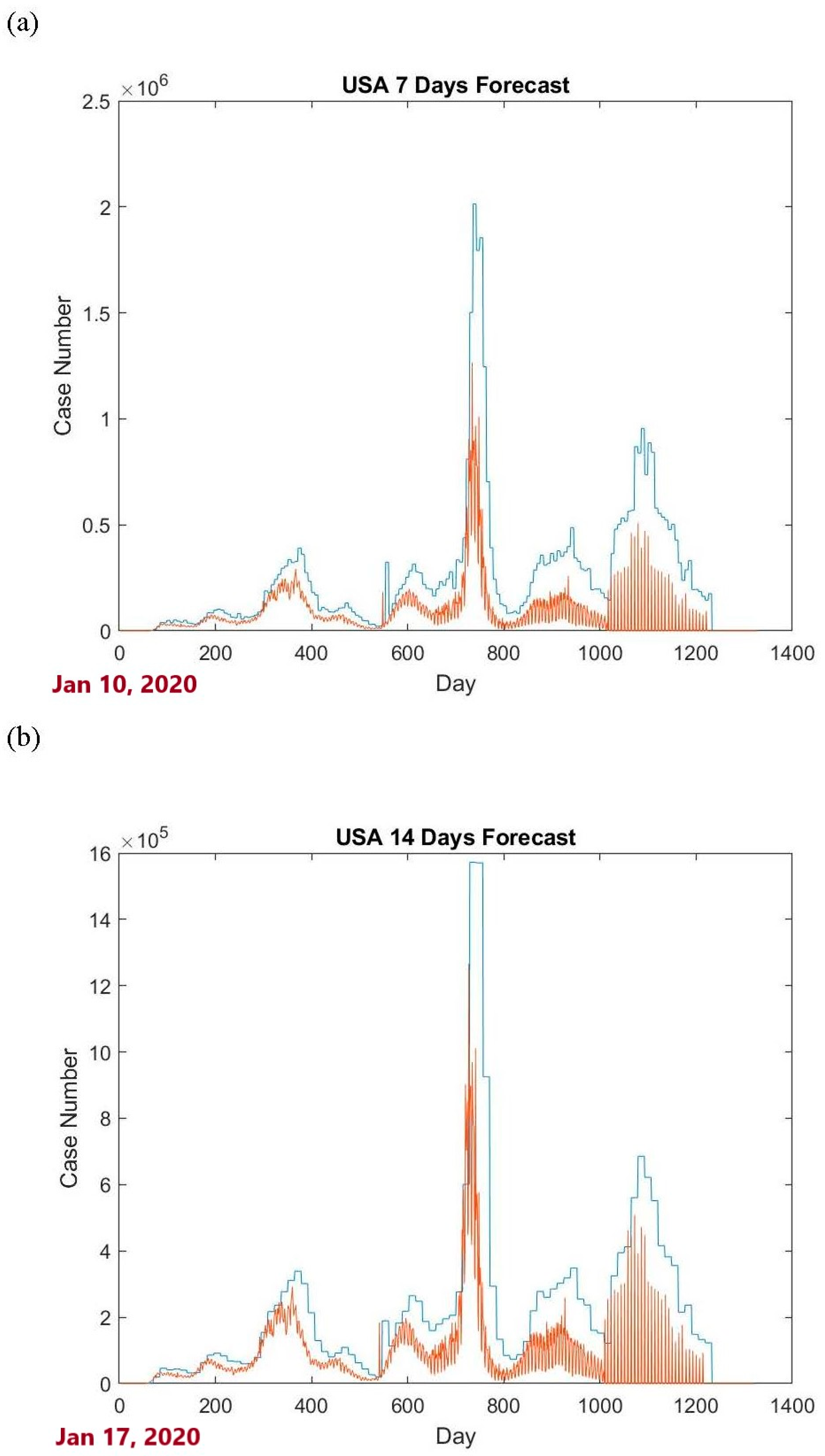
This is the upper tolerance bound for 24 January to 30 January. Similarly, the upper tolerance bounds for other days can be obtained. Figure 1 shows the upper tolerance bounds for the USA data case.

To evaluate the performance of the constructed upper tolerance bounds, the proportion of the number of COVID-19 cases that is lower than or equal to the upper tolerance bound is calculated. The proportion is defined as

$$r={\displaystyle \frac{\sum _{i=m}^{w}I(x_i\le u_i)}{w-m+1}}$$

(13)

where $I(·)$ denotes the indicator function.

Figure 1 shows that a large proportion of the data are below the calculated upper bounds. Since the upper bounds are the 0.99 content, 0.95 level upper tolerance bounds, it is expected that 99% of the data are below the constructed upper bounds. Using the criterion (13), for the 7-day and 14-day cases, the proportions are $r=0.9744$ and $r=0.9281$, respectively. This indicates a good outcome. However, these bounds have not yet achieved the original goal that 99% of daily new COVID-19 confirmed cases fall below them. To improve the outcomes, the confirmed case numbers from another country can be used as auxiliary information to aid in prediction.

3.3. Method Based on the Historical Data and Auxiliary Data Under the Normal Distribution

In addition to constructing the upper tolerance bound using historical data, auxiliary data from other regions can be utilized to enhance predictions. As we know, a new strain of COVID-19 may transmit from one country to another. It is likely that the data of one country are correlated with the past data from another country with a time lag. Therefore, if other regions have already experienced an outbreak, then the data may be useful in predicting the outbreak in another country. In this study, data from one of the two investigated countries, either the USA or the UK, are utilized as auxiliary data to aid in predicting the number of COVID-19 cases in the other country.

Different time lag cases can be considered when using the auxiliary data. Let $y_i$, $i=1,\dots ,w$ denote the daily data from another region. The time lag is denoted as $d.$ An appropriate time lag $d$ can be selected such that the absolute value of $\mathrm{c}\mathrm{o}\mathrm{r}\mathrm{r}\mathrm{e}\mathrm{l}\mathrm{a}\mathrm{t}\mathrm{i}\mathrm{o}\mathrm{n}(x_i,y_{i-d})$ is the largest based on historical data because the data $y_i$ is expected to provide earlier outbreak information for $x_i$. Then, the modified upper tolerance bound based on the historical data and auxiliary data using (6) can be calculated. The steps of calculating the upper tolerance bound using a 7-day timeframe are provided in Procedure 1.

Procedure 1

Step 1. Find a $d$ such that the absolute value of the $\mathrm{c}\mathrm{o}\mathrm{r}\mathrm{r}\mathrm{e}\mathrm{l}\mathrm{a}\mathrm{t}\mathrm{i}\mathrm{o}\mathrm{n} (x_i,y_{i-d})$ is large, say $d^{*}$.

Step 2. Consider a 7-day timeframe case using the data $\left(x_i,y_{i-d^{*}}\right), i=j+1,\dots , j+7.$ Calculate the estimators ${\widehat{\mu }}_x,{\widehat{\sigma }}_x,{\widehat{\mu }}_y$ and ${\widehat{\sigma }}_y$ for each $j$ based on these data.

Step 3. Let $y_{i-d^{*}}, i=j+8,\dots ,14,$ and the mean of these 7 $y$ values is denoted as ${\overline{y}}^{*}.$ And according to Theorem 1, calculate ${\rho }_{MAX}.$ Then calculate ${UTL}^{*}$ using formula (8) by replacing $y$ with ${\overline{y}}^{*}$.

Step 4. Use ${\widehat{\mu }}_x$ and ${\widehat{\sigma }}_x$ to calculate $UTL.$ Then take the maximum value of ${UTL}^{*}$ and $UTL$, which is the proposed upper tolerance bound ${UTL}^{**}$.

In Step 1 of Procedure 1, when not enough historical data are available, such as only the 7 or 14 days of data used, it is not easy to find the best $d^{*}$ value. In this case, we can consider the simple case by using $d=7$ when performing a 7-day timeframe scenario and using $d=14$ when performing a 14-day timeframe scenario. For the data used in this study, the entire dataset was used to find suitable $d^{*}$ values by calculating the correlation between the USA and UK data for different time lags, which shows that time lags of 7 and 14 are appropriate (

Table 2. The correlation analysis of the USA and UK datasets for different time lags.

Lag	1	2	3	4	5	6	7	8	9	10
Correlation	0.67	0.66	0.65	0.65	0.67	0.70	0.74	0.73	0.70	0.69
Lag	11	12	13	14	15	16	17	18	19	20
Correlation	0.68	0.69	0.71	0.74	0.72	0.69	0.66	0.65	0.64	0.66

).

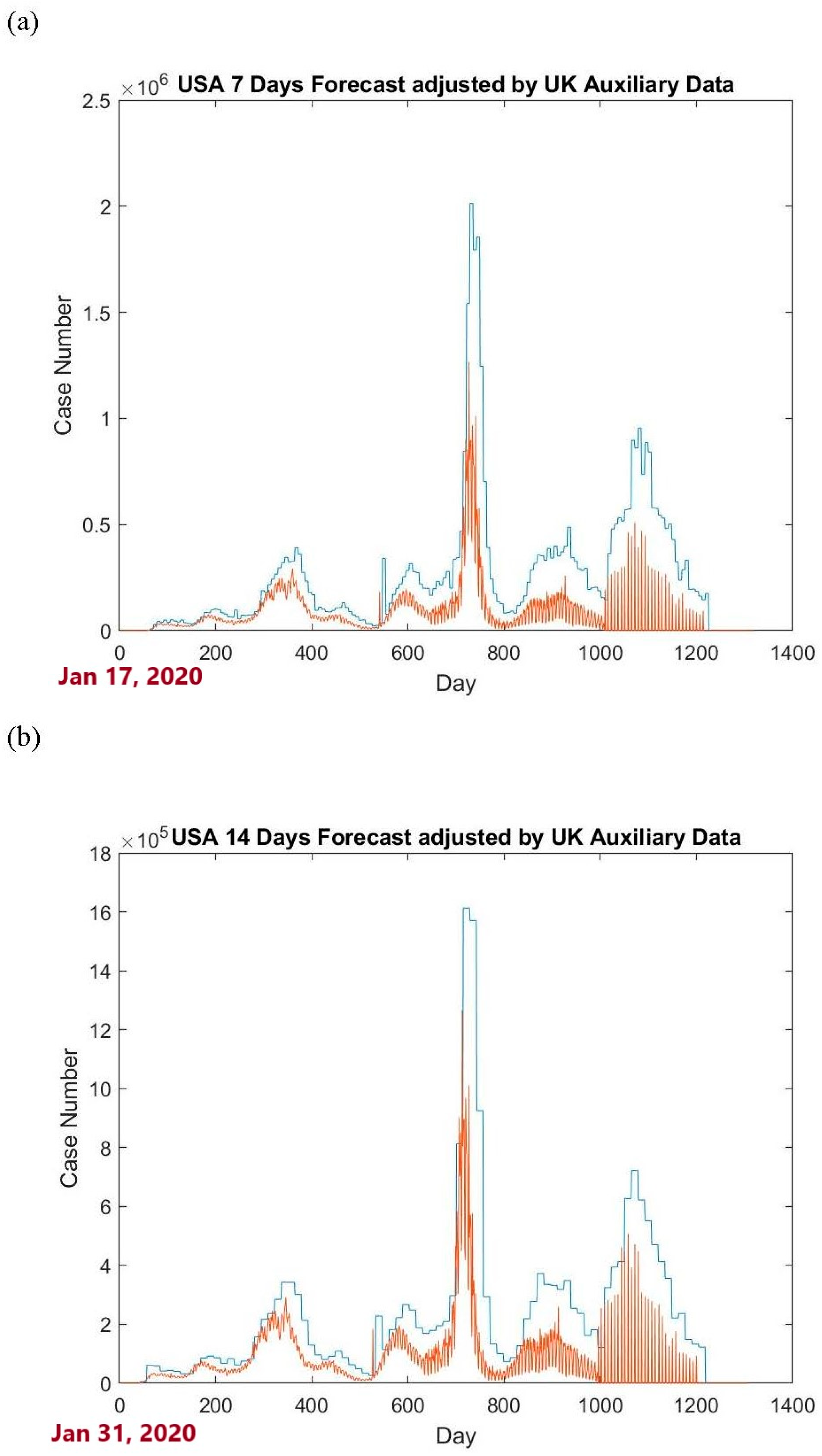
Consider the case with a time lag of 7 days, where UK historical data are used as auxiliary information to construct upper bounds for USA data. For a forecast period of 7 days, the past 7 days of USA data are used to calculate ${\widehat{\mu }}_X$ and ${\widehat{\sigma }}_X$, while the past 14–8 days of UK data are used to calculate ${\widehat{\mu }}_Y$ and ${\widehat{\sigma }}_Y$. The past 7 days of UK data are then used to calculate the mean, which is ${\overline{y}}^{*}$ in Step 3 of Procedure 1. For example, the 7-day USA data (7–13 February 2020) and the 7-day UK data (31 January to 6 February 2020) were used to calculate ${\widehat{\mu }}_x,{\widehat{\sigma }}_x,{\widehat{\mu }}_y$ and ${\widehat{\sigma }}_y$ for providing the USA 7-day (14–20 February 2020) upper tolerance bound. Through calculation, we have ${\widehat{\mu }}_X=0.1429,$ ${\widehat{\sigma }}_X=0.3780$, ${\widehat{\mu }}_Y=2.8571$ and ${\widehat{\sigma }}_Y=6.6940$. Note that the period of these UK data is 7 days before the period of these USA data. Then, the 7 UK data points (7–13 February 2020) are used to calculate ${\overline{y}}^{*}$ in Step 3 of Procedure 1. As a result, we have ${\overline{y}}^{*}=1.4286$ and ${\rho }_{MAX}=0.0464$. Then ${UTL}^{*}=1.8740$ and $UTL=1.8796$. The maximum value of ${UTL}^{*}$ and $UTL$ is 1.8796, which is the proposed upper tolerance bound for predicting the USA COVID-19 case numbers for the period (14–20 February 2020). The USA 7-day and 14-day forecasts incorporating auxiliary data from the UK are shown in Figure 2.

Table 3. The proportion of USA COVID-19 data below the upper bound.

Method	7 Days	14 Days
Upper bound based on USA historical data	0.9744	0.9281
Upper bound based on USA historical data and UK auxiliary data	0.9803	0.9526

and

Table 4. The proportion of UK COVID-19 data below the upper bound.

Method	7 Days	14 Days
Upper bound based on UK historical data	0.9624	0.8850
Upper bound based on UK historical data and USA auxiliary data	0.9720	0.9052

present the proportions of the case numbers below the calculated upper bounds for the USA and UK forecasts, respectively. For the USA case, as mentioned in Section 3.2, the proportions for the 7-day and 14-day forecasts based on the conventional upper tolerance bound are 0.9744 and 0.9281, respectively. When incorporating auxiliary data from the UK, the proportions for the 7-day and 14-day forecasts increase to 0.9803 and 0.9526, respectively.

Next, USA historical data are used as auxiliary information to incorporate historical data from the UK to construct upper bounds for predicting UK data. For the 7-day and 14-day forecasts, the proportions of the case numbers below the calculated upper bounds based on the conventional method are 0.9624 and 0.8850, respectively. When incorporating auxiliary data from the USA, the proportions for the 7-day and 14-day forecasts increase to 0.9720 and 0.9052, respectively.

Regarding the results presented in Table 3 and Table 4, while the proportions of the data below the upper bounds for these two methods do not reach 0.99, most of them are at least greater than 0.9. This means that these bounds can provide useful information for preparing sources for COVID-19 management.

3.4. Method Based on the Historical Data Under the Poisson Distribution

The proportions of the COVID-19 data below the upper bound based on the Poisson distribution for the USA and UK prediction are provided in

Table 5. The proportion of USA COVID-19 data below the upper bound based on the Poisson distribution.

Method	7 Days	14 Days
Upper bound (9)	0.5862	0.5870
Upper bound (10)	0.5877	0.5870

and

Table 6. The proportion of UK COVID-19 data below the upper bound based on the Poisson distribution.

Method	7 Days	14 Days
Upper bound (9)	0.5546	0.5386
Upper bound (10)	0.5546	0.5353

. The proportions are below 0.6, which is much lower than 0.99. This indicates that the normal distribution is more suitable to be used to construct upper tolerance limits for the COVID-19 data analysis than the Poisson distribution.

3.5. Method Based on the Historical Data Under the Negative Binomial Distribution

Table 7. The proportion of USA COVID-19 data below the upper bound based on the negative binomial distribution.

Method	7 Days	14 Days
Upper bound (11)	0.9428	0.8336
Upper bound (12)	0.9556	0.9115

and

Table 8. The proportion of UK COVID-19 data below the upper bound based on the negative binomial distribution.

Method	7 Days	14 Days
Upper bound (11)	0.9639	0.8056
Upper bound (12)	0.9789	0.9047

present the proportions of COVID-19 data falling below the upper bounds based on the negative binomial model for the USA and UK predictions. These proportions are much better than those from the Poisson distribution. Although the negative binomial distribution does not perform as well as the normal distribution, it remains a strong competitor.

4. Discussion

4.1. COVID-19 Studies

The global outbreak of COVID-19 had a profound and lasting impact on individuals and communities around the world. While some individuals may experience mild symptoms when infected with COVID-19, there is a possibility that it may be associated with serious comorbidities [24,25]. Vaccines have demonstrated high efficacy in preventing COVID-19 and its severe complications [26]. The administration of a two-dose vaccine has demonstrated high efficacy in preventing outbreaks and significantly reducing COVID-19 hospitalizations and fatalities [27]. To effectively prepare for and allocate sufficient supplies of vaccines or management, the accurate prediction of COVID-19 case numbers becomes a crucial factor for governments.

In the literature, various methods, such as machine learning, time series models, recurrent neural networks, regression models, global epidemic and mobility models, and more, have been employed to predict the number of COVID-19 cases [28]. The time-series regressive integrated moving average (ARIMA) model was applied to Johns Hopkins epidemiological data for predicting the trends in the prevalence and incidence of COVID-19 [29]. A cloud-based machine learning short-term forecasting model was developed to estimate the number of COVID-19-infected people over the following seven days in Bangladesh [30]. Different regression models have been applied to predict the number of COVID-19 confirmed cases [31]. A quasi-Poisson regression model was employed to forecast the confirmed case counts in Italy and Spain during lockdown [32]. A recurrent neural network model, specifically the modified Long Short-Term Memory model, was constructed to predict the number of newly affected individuals, losses, and recoveries in the upcoming days [33]. A time-dependent Susceptible–Infected–Recovered (SIR) model that tracks the transmission and recovery rate over time was employed to predict the trend of COVID-19 [34]. The Susceptible–Exposed–Infectious–Recovered (SEIR) epidemic model is widely used to study the spread of infectious diseases, and its compartmental variant, the l-i SEIR model, has been applied to analyze COVID-19 transmission trends [35]. Machine learning techniques were employed to predict a user’s COVID-19 infection status and raise awareness of individuals’ circumstances, potentially helping to prevent further spread of the disease [36].

In addition, the upper tolerance bound method has been successfully used as an upper limit of a control chart method to predict the start and end of a COVID-19 outbreak [13]. The control chart method is a useful tool that has been used to monitor COVID-19 cases [13,37,38,39]. The Shewhart control chart was developed to visualize and learn from variations in reported deaths during an epidemic of COVID-19 [37]. The control chart was also used to monitor COVID-19 or identify and analyze hotspot and coldspot regions of SARS-CoV-2 [38,39].

Differing from the majority of studies that primarily focus on predicting the number of COVID-19 cases, the proposed methods in this study aim to provide upper bounds that could be more useful in aiding in management preparation. A study more relevant to this paper is the COVID-19 Forecast Hub, which uses quantile ensembles that combine multiple models to improve accuracy and quantify uncertainty in predictions [40]. In addition, most of the prediction methods for COVID-19 data focus on using data from the same region to build models and predict the situation within that same region, rather than utilizing data from other regions as auxiliary for prediction [13,41,42,43]. The second proposed method in this study involves collaborating with data from other regions, and the results demonstrate that using data from other regions can enhance prediction accuracy.

4.2. Limitations

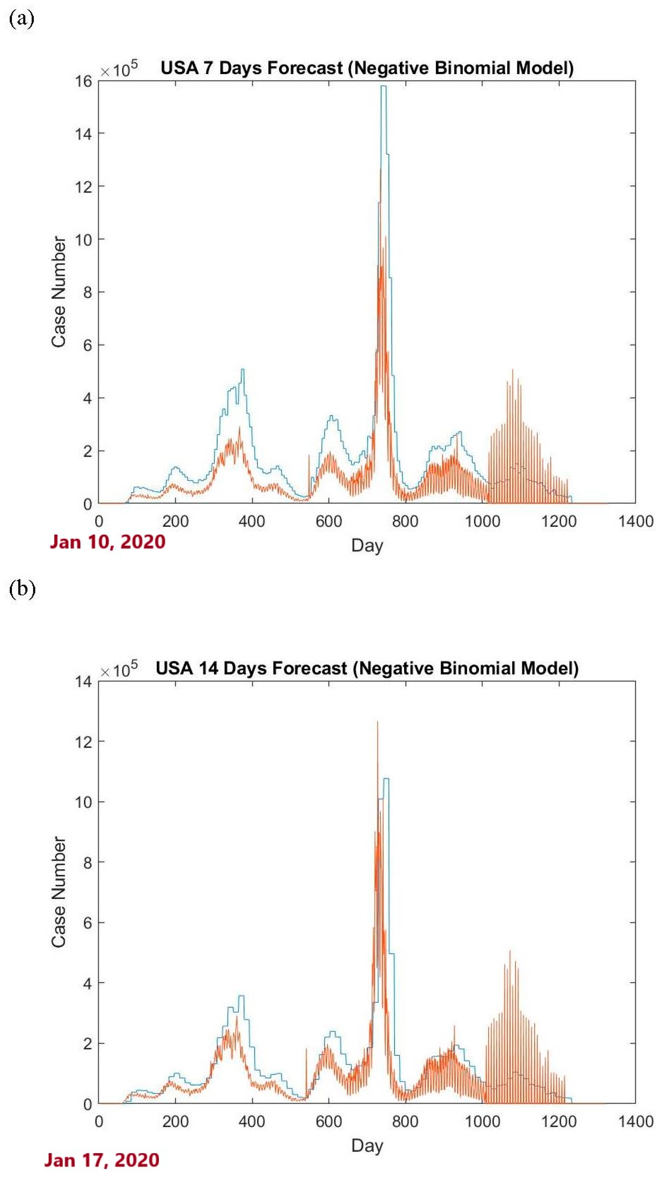
This study aims to provide upper bounds that can cover 99% of the daily new COVID-19 confirmed case numbers at a 0.95 confidence level. While the proposed methods cannot reach the nominal level of 0.99, in most cases for the datasets used in this study, the upper bounds derived from the normal distribution can cover at least 92% of the daily new COVID-19 confirmed case numbers. They can therefore serve as a useful reference for future pandemic management. However, from an economic perspective, it is also desirable that these upper bounds are not overly conservative to avoid resource waste. Figure 1 and Figure 2 show that the bounds derived from the normal distribution are much higher than the actual case numbers. In contrast, while the upper bounds derived from the negative binomial distribution are slightly lower than those from the normal distribution, Figure 3 shows that they are closer to the actual case numbers.

The conservativeness of these upper bounds can be measured by calculating the mean absolute distance from the upper bounds to the actual counts, relative to the mean of the actual counts, which is defined as

$$D={\displaystyle \frac{\sum _{i=m}^w|x_i-u_i|}{\sum _{i=m}^w{x}_i}}$$

(14)

The $D$ values for the three distribution cases are presented in

Table 9. The $D$ values of the upper bounds for the USA data.

Distributions		7 Days	14 Days
Normal	Historical data	2.18	1.78
	Historical data and auxiliary data	2.21	1.88
Poisson	Upper bound (9)	0.41	0.53
	Upper bound (10)	0.41	0.53
Negative Binomial	Upper bound (11)	1.19	0.80
	Upper bound (12)	2.39	1.33

.

Table 9 shows that the upper bounds derived from the normal distribution are slightly more conservative than those from the negative binomial distribution. While the upper bounds from the Poisson distribution have much smaller $D$ values compared to the other two distributions, Table 5 and Table 6 indicate that they cover less than 60% of the real data. Therefore, if conservativeness is considered, the upper bounds from the negative binomial distribution can be a good alternative to those from the normal distribution.

In addition, this paper focuses on using the exact β-content tolerance interval based on the normal, Poisson, and negative binomial distributions to provide an upper bound for daily new COVID-19 counts. Other tolerance interval methods, such as the bootstrap method and Bayesian tolerance interval methods, may be considered for future study.

5. Conclusions

This study employs tolerance interval methods to construct upper bounds for daily new COVID-19 case numbers, emphasizing forecasting predictive upper bounds rather than directly forecasting case numbers. In this framework, tolerance limits derived from several statistical models, including the normal, Poisson, and negative binomial distributions, are compared. Furthermore, auxiliary data are incorporated to enhance the coverage rates of the estimates. The findings indicate that some of the proposed tolerance limits can produce informative and reliable upper bounds for daily new COVID-19 counts. By focusing on bound estimation, this approach offers a valuable alternative to conventional forecasting methods that estimate the actual counts. Given that infectious diseases such as COVID-19 profoundly affect the United Nations Sustainable Development Goals, particularly those related to health systems and economic stability, the development of robust methods for pandemic preparedness is imperative. This study demonstrates that the proposed methods have the potential to improve pandemic preparedness through better equipment planning, resource allocation, and timely response strategies.

References

1. Wu, D.; Wu, T.; Liu, Q.; Yang, Z. The SARS-CoV-2 outbreak: What we know. Int. J. Infect. Dis. 2020, 94, 44–48. [Google Scholar] [CrossRef] [PubMed]
2. Chan-Yeung, M.; Xu, R.H. SARS: Epidemiology. Respirology 2003, 8, S9–S14. [Google Scholar] [CrossRef]
3. Ludwig, S.; Zarbock, A. Coronaviruses and SARS-CoV-2: A brief overview. Anesth. Analg. 2020, 131, 93–96. [Google Scholar] [CrossRef]
4. Lam, W.K.; Zhong, N.S.; Tan, W.C. Overview on SARS in Asia and the world. Respirology 2003, 8, S2–S5. [Google Scholar] [CrossRef]
5. Chen, Y.H.; Wang, H. Exploring Diversity of COVID-19 Based on Substitution Distance. Infect. Drug Resist. 2020, 13, 3887–3894. [Google Scholar] [CrossRef]
6. Dutta, A. COVID-19 waves: Variant dynamics and control. Sci. Rep. 2022, 12, 9332. [Google Scholar] [CrossRef]
7. Tao, K.; Tzou, P.L.; Nouhin, J.; Gupta, R.K.; de Oliveira, T.; Kosakovsky Pond, S.L.; Fera, D.; Shafer, R.W. The biological and clinical significance of emerging SARS-CoV-2 variants. Nat. Rev. Genet. 2021, 22, 757–773. [Google Scholar] [CrossRef]
8. Lin, L.; Zhao, Y.; Chen, B.; He, D. Multiple COVID-19 Waves and Vaccination Effectiveness in the United States. Int. J. Environ. Res. Public Health 2022, 19, 2282. [Google Scholar] [CrossRef]
9. Meeker, W.Q.; Hahn, G.J.; Escobar, L.A. Statistical Intervals: A Guide for Practitioners and Researchers; John Wiley & Sons: Hoboken, NJ, USA, 2017; Volume 541. [Google Scholar]
10. Ogunjo, S.T.; Fuwape, I.A.; Rabiu, A.B. Predicting COVID-19 Cases From Atmospheric Parameter Using Machine Learning Approach. Geohealth 2022, 6, e2021GH000509. [Google Scholar] [CrossRef]
11. Fatimah, B.; Aggarwal, P.; Singh, P.; Gupta, A. A comparative study for predictive monitoring of COVID-19 pandemic. Appl. Soft Comput. 2022, 122, 10880. [Google Scholar] [CrossRef]
12. Xu, L.; Magar, R.; Farimani, A.B. Forecasting COVID-19 new cases using deep learning methods. Comput. Biol. Med. 2022, 144, 10534. [Google Scholar] [CrossRef] [PubMed]
13. Wang, H. Tolerance limits for mixture-of-normal distributions with application to COVID-19 data. Wires Comput. Stat. 2023, 15, e1611. [Google Scholar] [CrossRef]
14. Jackson, M.T.; Medway, R.L.; Megra, M.W. Can Appended Auxiliary Data Be Used to Tailor the Offered Response Mode in Cross-Sectional Studies? Evidence from an Address-Based Sample. J. Surv. Stat. Methodol. 2021, 11, 47–74. [Google Scholar] [CrossRef]
15. McDonald, D.J.; Bien, J.; Green, A.; Hu, A.J.; DeFries, N.; Hyun, S.; Oliveira, N.L.; Sharpnack, J.; Tang, J.; Tibshirani, R. Can auxiliary indicators improve COVID-19 forecasting and hotspot prediction? Proc. Natl. Acad. Sci. USA 2021, 118, e2111453118. [Google Scholar] [CrossRef]
16. Reinhart, A.; Brooks, L.; Jahja, M.; Rumack, A.; Tang, J.; Agrawal, S.; Al Saeed, W.; Arnold, T.; Basu, A.; Bien, J.; et al. An open repository of real-time COVID-19 indicators. Proc. Natl. Acad. Sci. USA 2021, 118, e2111452118. [Google Scholar] [CrossRef]
17. Patel, J.K. Tolerance Limits-a Review. Commun. Stat. Theory 1986, 15, 2719–2762. [Google Scholar] [CrossRef]
18. Mee, R.W. β-expectation and β-content tolerance limits for balanced one-way ANOVA random model. Technometrics 1984, 26, 251–254. [Google Scholar] [CrossRef]
19. Krishnamoorthy, K.; Mathew, T. Statistical Tolerance Regions: Theory, Applications, and Computation; John Wiley & Sons: Hoboken, NJ, USA, 2009. [Google Scholar]
20. Natrella, M.G. Experimental Statistics Handbook 91; US Government Printing Office: Washington, DC, USA, 1963.
21. Natrella, M.G. Experimental Statistics; Courier Corporation: North Chelmsford, MA, USA, 2013. [Google Scholar]
22. Wang, H.; Tsung, F.G. Tolerance Intervals With Improved Coverage Probabilities for Binomial and Poisson Variables. Technometrics 2009, 51, 25–33. [Google Scholar] [CrossRef]
23. Cai, T.T.; Wang, H. Tolerance Intervals for Discrete Distributions in Exponential Families. Stat. Sin. 2009, 19, 905–923. [Google Scholar]
24. Wang, H. COVID-19, Anti-NMDA Receptor Encephalitis and MicroRNA. Front. Immunol. 2022, 13, 825103. [Google Scholar] [CrossRef]
25. Russell, C.D.; Lone, N.I.; Baillie, J.K. Comorbidities, multimorbidity and COVID-19. Nat. Med. 2023, 29, 334–343. [Google Scholar] [CrossRef] [PubMed]
26. Ellington, S.; Jatlaoui, T.C. COVID-19 vaccination is effective at preventing severe illness and complications during pregnancy. Lancet 2023, 401, 412–413. [Google Scholar] [CrossRef] [PubMed]
27. Crevecoeur, J.; Hens, N.; Neyens, T.; Lariviere, Y.; Verhasselt, B.; Masson, H.; Theeten, H. Change in COVID19 outbreak pattern following vaccination in long-term care facilities in Flanders, Belgium. Vaccine 2022, 40, 6218–6224. [Google Scholar] [CrossRef] [PubMed]
28. Shakeel, S.M.; Kumar, N.S.; Madalli, P.P.; Srinivasaiah, R.; Swamy, D.R. COVID-19 prediction models: A systematic literature review. Osong Public Health Res. Perspect. 2021, 12, 215–229. [Google Scholar] [CrossRef]
29. Benvenuto, D.; Giovanetti, M.; Vassallo, L.; Angeletti, S.; Ciccozzi, M. Application of the ARIMA model on the COVID-2019 epidemic dataset. Data Brief. 2020, 29, 105340. [Google Scholar] [CrossRef]
30. Satu, M.S.; Howlader, K.C.; Mahmud, M.; Kaiser, M.S.; Islam, S.M.S.; Quinn, J.M.W.; Alyami, S.A.; Moni, M.A. Short-Term Prediction of COVID-19 Cases Using Machine Learning Models. Appl. Sci-Basel 2021, 11, 4266. [Google Scholar] [CrossRef]
31. Ahmad, A.; Garhwal, S.; Ray, S.K.; Kumar, G.; Malebary, S.J.; Barukab, O.M. The Number of Confirmed Cases of Covid-19 by using Machine Learning: Methods and Challenges. Arch. Comput. Methods Eng. 2021, 28, 2645–2653. [Google Scholar] [CrossRef]
32. Tobias, A. Evaluation of the lockdowns for the SARS-CoV-2 epidemic in Italy and Spain after one month follow up. Sci. Total Environ. 2020, 725, 138539. [Google Scholar] [CrossRef]
33. Kumar, R.L.; Khan, F.; Din, S.; Band, S.S.; Mosavi, A.; Ibeke, E. Recurrent Neural Network and Reinforcement Learning Model for COVID-19 Prediction. Front. Public Health 2021, 9, 74410. [Google Scholar] [CrossRef]
34. Chen, Y.C.; Lu, P.E.; Chang, C.S.; Liu, T.H. A Time-Dependent SIR Model for COVID-19 With Undetectable Infected Persons. Ieee T Netw. Sci. Eng. 2020, 7, 3279–3294. [Google Scholar] [CrossRef]
35. Liu, X.; DeVries, A.C. Prediction of daily new COVID-19 cases-Difficulties and possible solutions. PLoS ONE 2024, 19, e0307092. [Google Scholar] [CrossRef]
36. Solayman, S.; Aumi, S.A.; Mery, C.S.; Mubassir, M.; Khan, R. Automatic COVID-19 prediction using explainable machine learning techniques. Int. J. Cogn. Comput. Eng. 2023, 4, 36–46. [Google Scholar] [CrossRef]
37. Perla, R.J.; Provost, S.M.; Parry, G.J.; Little, K.; Provost, L.P. Understanding variation in reported covid-19 deaths with a novel Shewhart chart application. Int. J. Qual. Health C 2021, 33, mzaa06. [Google Scholar] [CrossRef]
38. Mandal, S.; Roychowdhury, T.; Bhattacharya, A. Pattern of genomic variation in SARS-CoV-2 (COVID-19) suggests restricted nonrandom changes: Analysis using Shewhart control charts. J. Biosci. 2021, 46, 11. [Google Scholar] [CrossRef] [PubMed]
39. Hsu, C.-R.; Wang, H. EWMA Control Chart Integrated with Time Series Models for COVID-19 Surveillance. Mathematics 2025, 13, 115. [Google Scholar] [CrossRef]
40. Cramer, E.Y.; Huang, Y.; Wang, Y.; Ray, E.L.; Cornell, M.; Bracher, J.; Brennen, A.; Rivadeneira, A.J.C.; Gerding, A.; House, K. The United States COVID-19 forecast hub dataset. Sci. Data 2022, 9, 462. [Google Scholar] [CrossRef] [PubMed]
41. Hoque, A.; Malek, A.; Zaman, K. Data analysis and prediction of the COVID-19 outbreak in the first and second waves for top 5 affected countries in the world. Nonlinear Dyn. 2022, 109, 77–90. [Google Scholar] [CrossRef]
42. Pinter, G.; Felde, I.; Mosavi, A.; Ghamisi, P.; Gloaguen, R. COVID-19 Pandemic Prediction for Hungary; A Hybrid Machine Learning Approach. Mathematics 2020, 8, 890. [Google Scholar] [CrossRef]
43. Roda, W.C.; Varughese, M.B.; Han, D.; Li, M.Y. Why is it difficult to accurately predict the COVID-19 epidemic? Infect. Dis. Model. 2020, 5, 271–281. [Google Scholar] [CrossRef]
Figure 1. (a) Red line: the daily number of USA newly confirmed cases; blue line: the (0.99, 0.95) level upper tolerance bound based on the past 7-day data. The date of the x-axis starts from 10 January 2020. (b) Red line: the daily number of USA newly confirmed cases; blue line: the (0.99, 0.95) level upper tolerance bound based on the past 14-day data. The date of the x-axis starts from 17 January 2020.
Mathematics 13 02908 g001
Figure 2. (a) Red line: the daily number of USA newly confirmed cases; blue line: the (0.99, 0.95) level upper tolerance bound based on past 7-day and UK auxiliary data. The date of the x-axis starts from 17 January 2020. (b) Red line: the daily number of USA newly confirmed cases; blue line: the (0.99, 0.95) level upper tolerance bound based on past 14-day and UK auxiliary data. The date of the x-axis starts from 31 January 2020.
Mathematics 13 02908 g002
Figure 3. (a) Red line: the daily number of USA newly confirmed cases; blue line: the (0.99, 0.95) level upper tolerance bound based on the past 7 days using the negative binomial model. The date of the x-axis starts from 10 January 2020. (b) Red line: the daily number of USA newly confirmed cases; blue line: the (0.99, 0.95) level upper tolerance bound based on the past 14-day period using the negative binomial model. The date of the x-axis starts from 17 January 2020.
Mathematics 13 02908 g003