Regime-Switching Asset Allocation Using a Framework Combing a Jump Model and Model Predictive Control

Abstract

This study proposes a novel hybrid framework that integrates a jump model with model predictive control (JM-MPC) for dynamic asset allocation under regime-switching market conditions. The proposed approach leverages the jump model to identify distinct market regimes while incorporating a rolling prediction mechanism to estimate time-varying asset returns and covariance matrices across multiple horizons. These regime-dependent estimates are subsequently used as inputs for an MPC-based optimization process to determine optimal asset allocations. Through comprehensive empirical analysis, we demonstrate that the JM-MPC framework consistently outperforms an equal-weighted portfolio, delivering superior risk-adjusted returns while substantially mitigating portfolio drawdowns during high-volatility periods. Our findings establish the effectiveness of combining regime-switching modeling with model predictive control techniques for robust portfolio management in dynamic financial markets.

1. Introduction

Financial markets often exhibit distinct regimes due to major political–economic events or shifts in investor expectations [1]. These regime shifts can directly influence investment decisions and induce structural changes in asset correlations, posing new challenges for portfolio risk management [2].For instance, whereas bull markets—characterized by higher returns and lower volatility—encourage more aggressive strategies [3]. Regime-switching models have spurred growing research efforts to model market regime transitions mathematically.

Regime-switching models can be broadly categorized into parametric and non-parametric approaches, each exhibiting distinct methodological characteristics and financial applications [4]. Among parametric approaches, the hidden Markov model (HMM) [5] has proven particularly effective in capturing dynamic characteristics of financial time series ([6,7,8]). Extending beyond the HMM, researchers have developed alternative parametric models with different switching mechanisms, including the hidden semi-Markov state-switching (HSMS) model [9] and the spectral clustering HMM [10]. In contrast, non-parametric approaches employ data-driven techniques to identify latent regimes without imposing strong distributional assumptions. A significant advancement in this category is the jump model (JM) proposed by Bemporad et al. [11].Other innovative methods include trend filtering [12], K-means clustering [13], and recurrent neural networks [14], reflecting the increasing integration of machine learning into regime-switching analysis. Recent research by Tan and Wu [15] also provides a systematic comparison of various regime-switching models, highlighting their distinct mechanisms and empirical performance in financial time series analysis.

Regime-based asset allocation (RBAA) has emerged as a significant research focus in portfolio optimization.The study by Tu [16] demonstrated that regime-switching plays a critical role in portfolio decisions.Nystrup et al. [17] developed a dynamic optimization framework combining hidden Markov models (HMMs) with model predictive control (MPC), demonstrating RBAA’s superiority over static allocation in both returns and risk metrics. Costa and Kwon [18] developed a risk parity portfolio optimization model using a Markov regime-switching framework that adapts to changing market conditions to achieve higher long-term returns. Oprisor et al. [19] extended this approach by integrating HMMs into the Black–Litterman framework [20] for multi-period optimization, further validating RBAA’s effectiveness. Most recently, Shu et al. [21] incorporated asset-specific regime forecasts into Markowitz mean–variance optimization, highlighting the advantages of hybrid regime prediction methods in dynamic asset allocation.

Despite these advances, existing regime-aware allocation approaches still exhibit notable limitations: (i) most researchers only rely on parametric models such as the HMM, which may be less flexible in capturing complex and non-linear regime dynamics; (ii) multi-period optimization techniques, such as model predictive control (MPC), are rarely integrated with regime-switching models, leading to suboptimal adaptation to rapidly changing market conditions; and (iii) regime detection methods often overlook feature selection, risking the inclusion of redundant or noisy predictors that weaken forecasting accuracy. These gaps motivate the development of a more adaptive, data-driven, and multi-horizon framework.

To address these limitations, this study proposes a novel hybrid framework that integrates the jump model with model predictive control for dynamic multi-period asset allocation under regime-switching conditions. The JM enhances regime detection by jointly selecting relevant features and tuning hyperparameters through information criteria minimization. A rolling JM forecasting mechanism then produces multi-horizon predictions of expected returns and covariance matrices, which serve as dynamic inputs to the MPC optimizer. This integration enables both accurate regime identification and horizon-adaptive portfolio rebalancing, particularly during high-volatility market conditions.

The main contributions of this paper are as follows:

• Methodological innovation: We develop the first unified JM–MPC framework for regime-dependent multi-period portfolio optimization, embedding regime-switching forecasts directly into the MPC decision process.
• Enhanced regime identification: By employing the sparse jump model with feature selection, our approach identifies optimal predictors and hyperparameters, improving regime classification accuracy compared to conventional methods.
• Empirical robustness: Using a globally diversified multi-asset portfolio, we empirically show that JM–MPC outperforms an equal-weighted benchmark in risk-adjusted returns and drawdown control, especially during crises such as the COVID-19 pandemic.
• Practical relevance: The framework offers actionable guidance for institutional investors seeking resilient portfolio strategies under regime uncertainty.

The remainder of this paper is organized as follows: Section 2 details the methodological framework. Section 3 presents the empirical analysis including data selection, forecasting results, and backtesting evaluation, and Section 4 concludes with key findings and future research directions.

2. Methods

2.1. Regime Identification

The jump model (JM) is a non-parametric, data-driven approach for regime inference and parameter estimation. Bemporad et al. [11] provide a general objective function of the JM (Equation (1)). Equation (1) offers a flexible framework by incorporating a generic loss function ℓ, a parameter regularization term $r\left({\theta }_{S_k}\right)$, and a regime sequence penalty $\mathcal{L}\left(S\right)$. The choice of this objective function should balance the trade-off between fitting the given data and prior assumptions about the regime sequence $S_t$.

$$J(X,\Theta ,S)=\sum _{t=1}^T\mathsf{\ell }(X_t,{\theta }_{S_t})+\sum _{k=1}^{K}r\left({\theta }_{S_k}\right)+\mathcal{L}\left(S\right)$$

(1)

Building on the assumption of the persistence of the regime sequence, Shu et al. [4] proposed a regularized objective function. Equation (2)) uses squared-error loss (Equation (3)), which is smooth and convex in $\Theta$. The regime sequence penalty is non-smooth and non-convex due to the discrete indicator function $\mathbb{I}\{S_t\ne S_{t+1}\}$, making the objective non-smooth and non-convex overall. Jump penalty coefficient $\lambda \ge 0$ is a hyperparameter that balances the stability of regime transitions.The optimal $\Theta$ and $S_t$ can be estimated by minimizing Equation (2) through coordinate descent and dynamic programming [22].

$$J^{*}(X,\Theta ,S)=\sum _{t=1}^T\mathsf{\ell }(X_t,{\theta }_{S_t})+\lambda \sum _{t=1}^{T-1}\mathbb{I}\{S_t\ne S_{t+1}\}$$

(2)

$$\mathsf{\ell }(x,\theta )={\displaystyle \frac{1}{2}}{\parallel x-\theta \parallel }_2^2$$

(3)

where $X\equiv {\left\{X_t\right\}}_{t=1}^T$ denotes the observed feature sequence and $\Theta \equiv {\left\{{\theta }_k\right\}}_{k=1}^K$ represents the set of regime-specific parameters.

Since the JM operates on feature sequences, an important consideration is the selection of informative features.Nystrup et al. [23] extended this framework by introducing the sparse jump model (SJM), which incorporates a feature selection mechanism that maximizes the weighted between-cluster sum of squares (BCSS) criterion proposed by Witten and Tibshirani [24]. Formally, the SJM solves the following constrained optimization problem (Equation (4)) to determine optimal feature weights. In our framework, the SJM is used to enhance JM fitting by improving regime identification accuracy and selecting the most discriminative features and optimal hyperparameters.

$$\begin{array}{cc}\hfill & \underset{w\in {\mathbb{R}}^p}{max}\left\{w^{\top }\sum _{k=1}^K\left|n_k\right|{({\theta }_k-\overline{\theta })}^2-\lambda \sum _{t=1}^T{\mathbb{I}}_{s_t\ne s_{t+1}}\right\}\hfill \\ \hfill & {\mathrm{subject}\mathrm{to}:\parallel w\parallel }_2^2\le 1,{\parallel w\parallel }_1\le \kappa ,w_p\ge 0\forall p\hfill \end{array}$$

(4)

where $\kappa \in [1,\sqrt{p}]$ serves as a sparsity-tuning parameter. Notably, the standard JM emerges as a special case when uniform feature weights ($w_1=\dots =w_p$) are applied.

In our empirical analysis, the feature vector $X_t$ is constructed from a comprehensive set of financial variables, including technical indicators, fundamental macroeconomic factors, and market sentiment proxies. The specific features and their transformations are detailed in Section 3.2. The optimized hyperparameter $\lambda$ and feature weights w, obtained through the SJM procedure, are presented in Section 3.3.

2.2. JM Rolling Forecast

Building on the regime-identification framework established by JM, we develop a rolling financial forecasting system that incorporates regime information. Consider an asset return series ${\left\{r_t\right\}}_{t=1}^T$ with K latent regimes, where returns in each state follow a Gaussian distribution. Within each rolling window of size w, the JM estimation procedure takes as input the predefined feature sequences and hyperparameters from the SJM and produces four key outputs: (i) regime-specific parameter estimates (${\mu }_s,{\sigma }_s^2$), (ii) the inferred state sequence ($s_t$), (iii) time-varying state probabilities ($q_t\in {[0,1]}^K$), and (iv) the state-transition probability matrix ($\Gamma \in {[0,1]}^{K\times K}$).

$$r_t\sim N({\mu }_s,{\sigma }_s^2)s\in \{1,2,\dots ,K\}$$

(5)

Using the four regime-conditioned parameters at time t, we compute the unconditional moments for $t+1$ through probabilistic aggregation. First, the unconditional expected return can be estimated as the probability-weighted average of conditional returns across different regimes, where the weights correspond to the state probabilities. Then, the unconditional covariance matrix comprises two components: the within-state variance that captures intrinsic return volatility in each regime and the additional variance induced by return prediction discrepancies across regimes.

$${\widehat{q}}_{t+1}=q_t·\Gamma$$

(6)

$${\widehat{\mu }}_{t+1}=\sum _s{\widehat{q}}_{t+1}·{\mu }_s$$

(7)

$${\widehat{\sigma }}_{t+1}^2=\sum _s{\widehat{q}}_{t+1}·{\sigma }_s^2+\sum _s{\widehat{q}}_{t+1}·({\mu }_s-{\widehat{\mu }}_{t+1}){({\mu }_s-{\widehat{\mu }}_{t+1})}^{\prime }$$

(8)

The rolling forecast framework proposed above supports two key extensions: (i) multi-horizon prediction through iterative H-step-ahead forecasting across rolling windows and (ii) multi-asset portfolios by replacing scalar variance ${\sigma }_s^2$ with full covariance matrices ${\Sigma }_s\in {\mathbb{R}}^{N\times N}$.

$${\widehat{\Sigma }}_{t+1}=\sum _s{Q}_{t+1}·{\Sigma }_s+\sum _s{Q}_{t+1}·({\mu }_s-{\widehat{\mu }}_{t+1}){({\mu }_s-{\widehat{\mu }}_{t+1})}^{\prime }$$

(9)

where N represents the number of assets in a portfolio, $Q_t\in {\mathbb{R}}^{K\times N}$ is a state probability vector, and ${\Sigma }_s$ is the conditional regime covariance.

In our empirical analysis, the optimal regime sequence $S_t$ and the estimated regime parameters—including ${\mu }_s$, ${\sigma }_s^2$, $q_t$, and $\Gamma$—are derived from the asset training data and presented in Section 3.4.1. The rolling forecasts of expected returns (${\widehat{\mu }}_{t+1}$) across different assets are illustrated in Section 3.4.2.

2.3. MPC Optimization

Model predictive control (MPC) is a stochastic optimization method that solves multi-period portfolio problems by dynamically adjusting weights based on predicted returns and risk [25]. The optimal weight allocation across time periods is obtained by solving the following optimization problem:

$$\underset{w_{t+1},\dots ,w_{t+H}}{max}\sum _{\tau =t+1}^{t+H}{\widehat{\mu }}_{\tau |t}^{\top }{w}_{\tau }-{\widehat{\varphi }}_{\tau |t}^{\mathrm{trade}}(w_{\tau }-w_{\tau -1})-{\widehat{\varphi }}_{\tau |t}^{\mathrm{hold}}\left(w_{\tau }\right)-\gamma {\widehat{\psi }}_{\tau |t}\left(w_{\tau }\right)$$

(10)

where $w_{t+1},\dots ,w_{t+H}$ represent the optimal portfolio weights over the H-step horizon; $\widehat{\mu }\tau |t$ denotes the conditional expected returns; $\widehat{\varphi }{\tau |t}^{\mathrm{trade}}$ and $\widehat{\varphi }{\tau |t}^{\mathrm{hold}}$ are transaction and holding costs functions, respectively; $\gamma$ is the risk aversion coefficient; and $\widehat{\psi }\tau |t$ is the risk function.

In this study, we replace ${\widehat{\mu }}_{\tau |t}$ with the JM rolling forecasts of expected returns. Following Boyd et al. [26], we formulate a convex optimization problem for MPC, as presented in Equation (11). Here, both transaction and holding costs are modeled as LASSO penalty functions on asset weights, in line with the methodology of Li et al. [27]. For the risk function, we adopt the standard mean–variance framework [28], where the portfolio risk is estimated using the JM rolling forecasts of the asset return covariance matrix. We implement the following portfolio constraints on asset weights: (i) non-negative weights (prohibiting short selling), (ii) a 40% maximum allocation limit per asset, and (iii) a full investment requirement where portfolio weights sum to unity.

$$\begin{array}{cc}\hfill & \underset{w_{t+1},\dots ,w_{t+H}}{max}\sum _{\tau =t+1}^{t+H}{\widehat{\mu }}_{\tau |t}^{\prime }{w}_{\tau }-\kappa {∥w_{\tau }-w_{\tau -1}∥}_1-\rho {∥w_{\tau }∥}_1-\gamma w_{\tau }^{\prime }{\widehat{\Sigma }}_{\tau |t}{w}_{\tau }\hfill \\ \hfill & \mathrm{subject}\mathrm{to}:0\le w_{\tau }\le 0.4,\forall \tau =t+1,\dots ,t+H\hfill \\ \hfill & \sum _i{w}_{\tau }=1,\forall \tau =t+1,\dots ,t+H\hfill \end{array}$$

(11)

where $\kappa$ denotes the transaction cost penalty coefficient, $\rho$ represents the holding cost penalty coefficient, and ${\Sigma }_{\tau }$ corresponds to the time-varying covariance matrix of asset returns.

Algorithm 1 outlines the four key steps in the MPC approach for multi-period portfolio optimization. In our study, Step 1 and Step 2 are replaced with JM rolling forecasts.In practical computation, we utilize the open-source Python package CVXPortfolio (https://github.com/cvxgrp/cvxportfolio (accessed on 15 August 2015)) developed by Body et al. [26] to optimize portfolios.

Algorithm 1: MPC approach to multi-period portfolio selection [17]

1. Update model parameters based on the most recent observation; 2. Forecast future values of all unknown quantities H steps into the future; 3. Compute the optimal sequence of weights $w_{t+1}^{*},\dots ,w_{t+H}^{*}$ based on the current portfolio $w_t$; 4. Execute the first trade $w_{t+1}^{*}-w_t$ and return to Step 1.

The aforementioned MPC optimization procedure is implemented in our empirical study. The resulting optimal hyperparameters ($\kappa$, $\rho$, $\gamma$) and the corresponding portfolio allocation weights w, obtained for different prediction horizons H, are presented and discussed in Section 3.5.

2.4. JM-MPC Framework

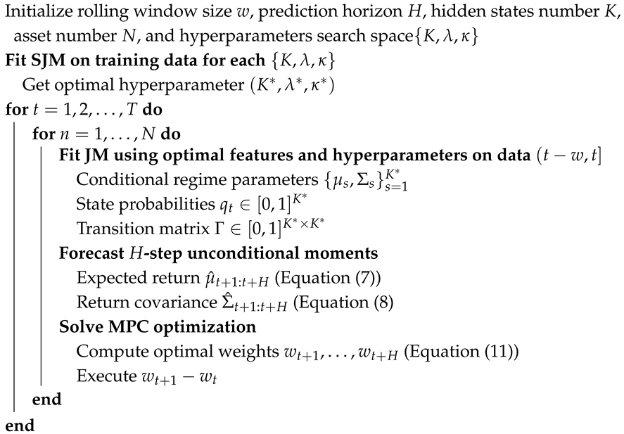
This study introduces a novel dynamic asset allocation framework that integrates market regime forecasting from the jump model (JM) with model predictive control (MPC). As detailed in Algorithm 2, the JM-MPC framework operates through four sequential stages:

• Optimal Feature and Hyperparameter Selection: Building upon the framework developed by Cortese et al. [29], we implement the sparse jump model (SJM) coupled with information criteria to jointly optimize feature selection and hyperparameters. In our empirical analysis, we employ grid search techniques to determine three key hyperparameters: (i) the number of market regimes K, (ii) the penalty coefficient $\lambda$, and (iii) feature space dimensionality $\kappa$.
• Regime-Dependent Estimation: For each rolling window, the JM fits regime-specific parameters using optimal features and hyperparemeters from the SJM, including the conditional mean (${\mu }_s$), conditional covariance (${\Sigma }_s$), regime probabilities ($q_t$), and transition probability matrix ($\Gamma$).
• Multi-Period Forecasting: Through iterative application of the regime transition matrix $\Gamma$, the framework projects H-period unconditional asset moments—the expected return vector (${\widehat{\mu }}_{t+1:t+H}$) and covariance matrix (${\widehat{\Sigma }}_{t+1:t+H}$) for MPC optimization.
• Adaptive MPC Optimization: MPC solves a convex optimization problem to determine optimal weights $\{w_{t+1},\dots ,w_{t+H}\}$, then executes only the immediate trade ($w_{t+1}-w_t$) before re-estimating at $t+1$.

Algorithm 2: JM-MPC rolling estimation for asset allocation

2.5. Computational Complexity of JM-MPC

The JM-MPC algorithm exhibits polynomial-time complexity, making it suitable for large-scale asset allocation problems. The computational cost is dominated by three key steps:

• Regime-Dependent Estimation: The jump model requires $O(K^2·w·N)$ operations per window, where K is the number of regimes, w is the rolling window size, and N is the number of assets. This step involves estimating regime-specific parameters $({\mu }_s,{\Sigma }_s)$, state probabilities $\left(q_t\right)$, and the transition matrix $(\Gamma )$.
• Multi-Period Forecasting: Projecting H-step returns and covariances scales as $O(K^2·H·N^2)$ involves iteratively applying $\Gamma$ and compounding regime-dependent moments.
• MPC Optimization: The convex optimization problem in Equation (11) involves $H·N$ variables, with a worst-case complexity of $O(H^3·N^3)$ due to quadratic programming. While this remains tractable for moderate H (e.g., $H\le 30$), longer horizons (e.g., $H=100$) can become computationally demanding. To address this, distributed optimization techniques such as the alternating direction method of multipliers (ADMM) [30] can be employed, enabling parallelized solutions across multiple processors and significantly improving scalability.

The overall complexity is $O(T·(K^2·w·N+K^2·H·N^2+H^3·N^3))$, where T is the number of rolling steps. Crucially, all terms grow polynomially with problem size, and the use of distributed methods for MPC ensures feasibility even for high-dimensional portfolios or long prediction horizons.

2.6. Comparative Advantages over Existing Approaches

The proposed JM-MPC framework offers several key advantages over existing approaches in the regime-based asset allocation literature. First, while many existing studies rely on parametric models such as the hidden Markov model (HMM) for regime identification ([19,27]), the JM-MPC framework employs a non-parametric jump model to capture market regimes. This approach eliminates the need for predefined state-transition structures and distributional assumptions, thereby offering greater flexibility in identifying complex, data-driven regime dynamics and reducing model specification risks. Furthermore, by integrating model predictive control with regime forecasts, JM-MPC enables dynamic multi-period optimization that explicitly incorporates time-varying risk and return expectations, a capability generally absent in conventional HMM-based strategies.

Second, while existing studies often apply the jump model without incorporating explicit feature selection mechanisms [4], this work introduces a structured feature selection framework through the sparse jump model to identify the most discriminative predictors for regime identification, thereby significantly enhancing both model interpretability and robustness. Furthermore, most current research on the jump model focuses primarily on regime identification and forecast [21]; our study extends its application by proposing a novel rolling return forecasting framework that integrates regime information for multi-period predictive modeling.

3. Empirical Analysis

3.1. Data

In this section, we empirically evaluate our JM-MPC hybrid framework introduced in Section 2. Through systematic backtesting on real asset data, we validate the framework’s ability to identify market regimes and optimize portfolio decisions by comparing its performance with basic portfolio strategies while explicitly linking the theoretical state variables to their empirical counterparts in the analysis.

We constructs a diversified portfolio spanning multiple asset classes, including equities, bonds, commodities, and real estate. Representative financial assets from both developed and emerging markets were selected, with each major asset class subdivided into risk- and return-based subcategories, yielding a total of twelve assets. Each subcategory is proxied by a corresponding benchmark index, and price movements are tracked using exchange-traded funds (ETFs) that replicate these indices. The specific ETF classifications are detailed in

Table 1. Asset classes and underlying assets.

Category	Asset	Index Name	ETF Ticker
Equity	US Large-Cap Equity	S&P 500 Index	IVV
	US Mid-Cap Equity	S&P MidCap 400 Index	IJH
	US Small-Cap Equity	Russell 2000 Index	IWM
	Developed Markets ex-US Equity	MSCI Developed Markets Index	EFA
	Emerging Markets Equity	MSCI Emerging Markets Index	EEM
Bonds	US Treasury Bonds	U.S. Long-Term Treasury Index	TLT
	US High-Yield Bonds	U.S. High-Yield Bond Index	HYG
	US Corporate Bonds	U.S. Corporate Bond Index	SPBO
Futures	Commodities	DBIQ Diversified Commodity Index	DBC
	Precious Metals	LBMA Gold Index	GLD
	Crude Oil	WTI Crude Oil	USO
Real Estate	US Real Estate	Dow Jones U.S. Real Estate Index	IYR

.

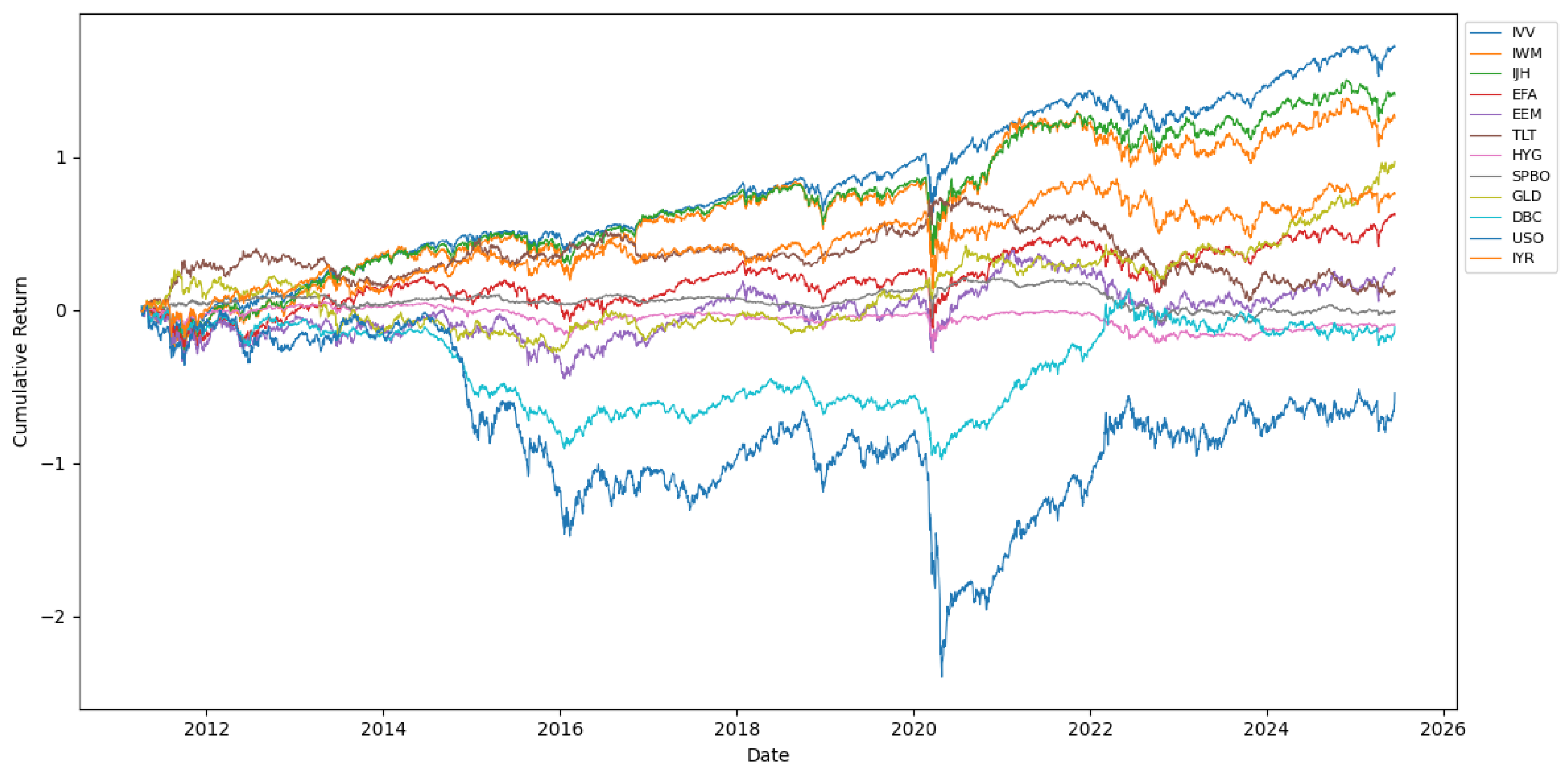
We obtained daily ETF price data for the selected assets from 2011 to 2025 using the Bloomberg Terminal. Additionally, we employ the US three-month Treasury constant maturity yield as a proxy for the risk-free rate, sourced from the Federal Reserve Economic Data (FRED) database. Daily cumulative returns of the asset ETF were derived from their closing prices, as shown in Figure 1.

The cumulative return curves of various ETF assets depicted in Figure 1 reveal several key insights. Among the equity ETFs, emerging markets (EEM) exhibit relatively low correlations with developed markets (EFA and IVV). Specifically, during the COVID-19 market crash in early 2020, nearly all assets experienced sharp drawdowns. Furthermore, most assets exhibited prolonged bullish or bearish trends, reinforcing the value of regime-based investing for portfolio optimization.

Table 2. Historical performance statistics of different assets.

ETF	Excess Return	Volatility	Sharpe Ratio	Maximum Drawdown	Calmar Ratio
IVV	0.0967	0.1759	0.5495	0.3390	0.2852
IJH	0.0659	0.2044	0.3223	0.4218	0.1562
IWM	0.0493	0.2235	0.2209	0.4226	0.1168
EFA	0.1383	0.1827	0.7576	0.3820	0.0362
EEM	−0.0165	0.2131	−0.0775	0.4372	−0.0377
TLT	−0.0165	0.1524	−0.1083	0.5175	−0.0319
HYG	−0.0233	0.0858	−0.2719	0.2872	−0.0812
SPBO	−0.0171	0.0751	−0.2276	0.2639	−0.0648
DBC	−0.0344	0.1716	−0.2006	0.6710	−0.0513
GLD	0.0450	0.1562	0.2884	0.4555	0.0899
USO	−0.1098	0.3605	−0.3046	0.9528	−0.1152
IYR	0.0198	0.1988	0.0996	0.4232	0.0468

Note: All indicators are annualized metrics calculated based on 252 trading days per year.

shows the annualized asset performance for the evaluation period running from April 2011 to June 2025, which highlights that there is a clear difference in the performance across different assets. While equities like EFA delivered strong returns (Sharpe ratio = 0.76), bonds (TLT and HYG) and commodities (DBC and USO) underperformed with negative Sharpe ratios. Notably, USO suffered extreme losses, highlighting the risks in energy markets. These results emphasize the need for careful asset selection, especially as traditional safe havens like bonds struggled during this period.

3.2. Feature Engineering

Table 3. List of features to fit the SJM.

Feature	Transformation	Window Lengths	Abbreviation
Category: Technical
Returns	EWMA	5, 21, 63	$EWMA{\left(r\right)}_w$
Downside Deviation	log	5, 21, 63	$D{D}_w$
Sortino Ratio	-	5, 21, 63	$Sortin{o}_w$
RSI	-	5, 21, 63	$RS{I}_w$
CCI	-	5, 21, 63	$CC{I}_w$
MACD	-	(5, 21), (21, 63)	$MAC{D}_{s,l}$
Bolling Bands	-	5, 21, 63	$B{B}_w$
Stochastic Oscillator	-	5, 21, 63	$\%K_w$
Category: Fundamental
US 10Y Yield	EWMA	5, 21, 63	$10Y_w$
US 2Y Yield	EWMA	5, 21, 63	$2Y_w$
Category: Sentiment
VIX Index	log, EWMA	5, 21, 63	$VI{X}_w$

Note: Window lengths (5, 21, 63) correspond to approximately 1 week, 1 month, and 3 months of trading days, respectively, based on an average of 252 trading days per year.

provides a detailed description of all features used as inputs to the SJM, categorized into three types: technical, fundamental, and investor sentiment indicators. Technical indicators, which are derived from historical returns, serve as important measures of risk. These include the exponentially weighted moving average (EWMA), downside deviation (DD), and the Sortino ratio (SR), according to Shu et al. (2024) [4], as well as several widely-used indicators such as MACD, RSI, CCI, Bollinger Bands (BBs), and the stochastic pscillator (%K) to capture price trends and momentum. These indicators have been demonstrated to effectively identify regimes in cryptocurrency markets [29]. Fundamental and sentiment indicators also play a critical role in reflecting the broader market environment [31]. We use the 10-year and 2-year U.S. Treasury yields and the VIX index, which were sourced from the FRED database, as proxies for these categories. All indicators are calculated over three time windows (one week, one month, and one quarter) to enhance robustness and adaptability.

$$DD=\sqrt{{\displaystyle \frac{1}{T}}{\sum }_{t=1}^{T}max{(0,-r_i)}^2}$$

(12)

$$SR={\displaystyle \frac{\overline{r}}{DD}}$$

(13)

Figure 2 illustrates the historical closing prices of the VIX index and U.S. Treasury yields. A pronounced spike in the VIX during the initial phase of the COVID-19 pandemic in 2020 reflects a period of extreme market fear. Concurrently, Treasury yields declined sharply—most notably the 10-year yield—indicating strong flight-to-safety behavior. These variables can jointly support empirical regime identification in financial markets.

3.3. Hyperparameter and Feature Selection

The jump model requires the optimization of three key hyperparameters: the number of market states (K), the jump penalty coefficient ($\lambda$), and the feature count ($\kappa$). Using a grid search approach with candidate values (

Table 4. Initial hyperparameter lists.

Hyperparameters	Value
K	2, 3, 4, 5
$\lambda$	0, 5, 10, 25, 50, 100
$\kappa$	2, 3, 4, 5, 6, 7, 8

), we identify the optimal hyperparameter combination for fitting the SJM. Following Cortese et al. (2024) [29], we employ information-theoretic criteria—including the Akaike information criterion (AIC), the Bayesian information criterion (BIC), and the focused information criterion (FTIC)—to select hyperparameters that optimally balance model fit against parametric complexity.

First, we construct the aforementioned feature sequences using asset closing prices and daily returns. These sequences, combined with candidate hyperparameter combinations $\{K,\lambda ,\kappa \}$, serve as inputs for the SJM fitting procedure. For each hyperparameter set, we compute and record both the information criterion (IC) values and their corresponding feature weights.

Table 5. Optimal hyperparameter grid search results for different assets.

Asset Class	K	$\mathit{\kappa }$	$\mathit{\lambda }$	AIC	BIC	FTIC
IVV	3	5	100	2.6263	3.7398	3.8646
IJH	3	5	100	4.1234	5.5678	6.8901
IWM	4	5	100	1.4567	2.7890	3.2345
EFA	3	5	100	3.9012	4.5678	5.4321
EEM	3	5	100	5.6789	6.1234	7.8901
TLT	2	5	100	2.3456	3.8901	4.5678
HYG	2	5	100	6.7890	7.2345	8.1234
SPBO	2	5	100	3.4567	4.8901	5.6789
DBC	3	5	100	7.8901	8.3456	9.1234
GLD	4	5	100	4.5678	5.1234	6.7890
USO	3	5	100	8.2345	9.6789	7.4567
IYR	2	5	100	5.9012	6.3456	7.8901

presents the grid search results across various asset classes. The findings indicate distinct latent regime characteristics among different risk categories: equities and commodities predominantly require 3–4 hidden states, whereas lower-risk assets such as bonds and real estate achieve optimal fit with fewer states. This pattern reflects structural differences in their risk–return architectures. Additionally, all assets consistently exhibit optimal performance under the parameter values of $\lambda =100$ and $\kappa =5$.

Figure 3 illustrates the feature importance across different asset classes. VIX-related sentiment features dominate for equities and commodities, aligning with volatility feedback effects, while features related to Treasury yield curves prove most predictive for bonds and real estate, reflecting the influence of macroeconomic fundamentals. Notably, downside risk (DD) and Bollinger Bands outperform other technical features consistently across all asset classes, suggesting that markets price asymmetric risks more uniformly than symmetric technical patterns. These results demonstrate that the SJM effectively captures both asset-class-specific drivers and universal technical factors in financial markets.

3.4. JM Fitting

3.4.1. Regime Identification

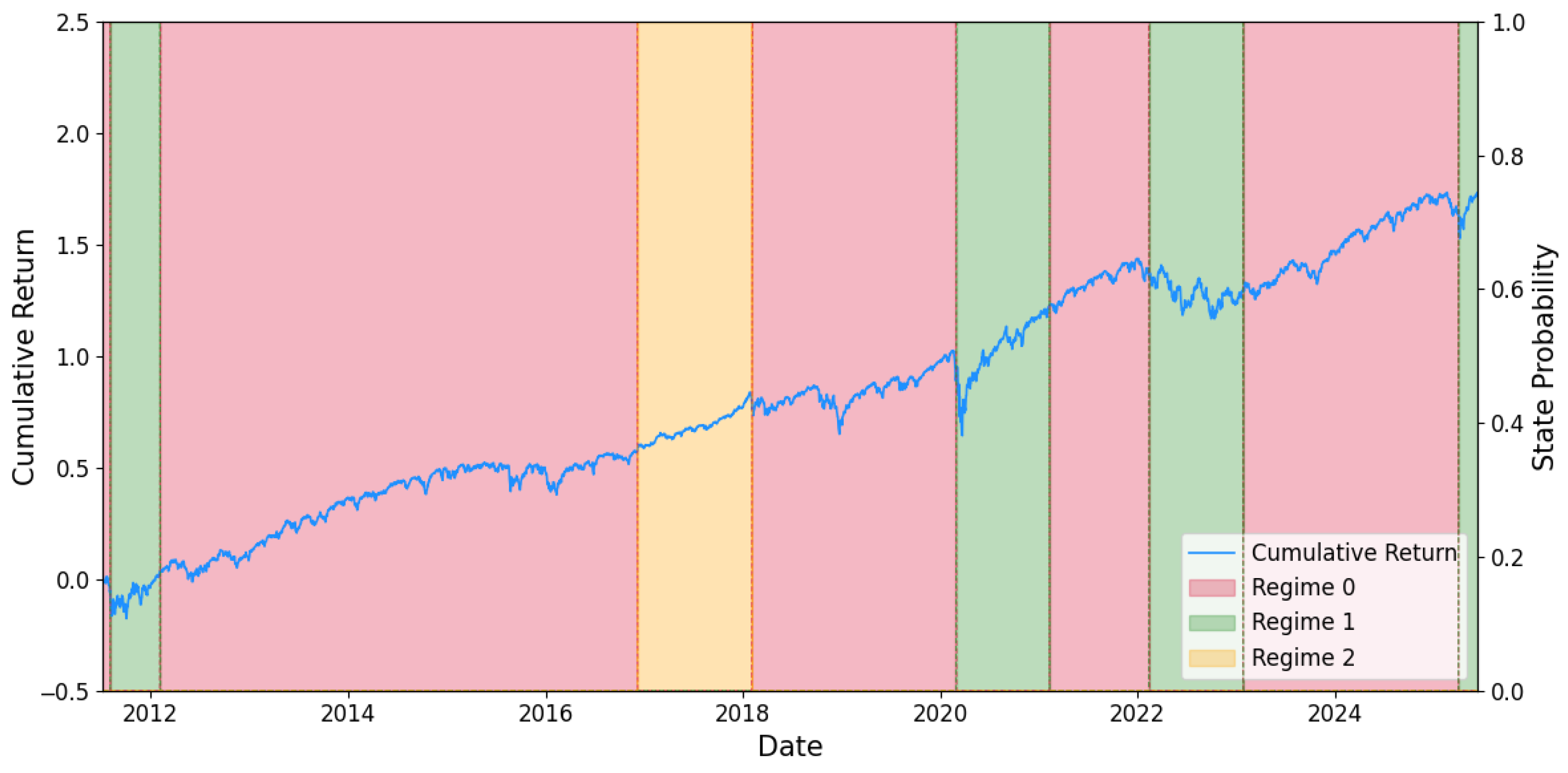
Based on the optimal hyperparameters and feature selection results obtained for different assets, this study employs the JM to identify historical latent market regimes for each asset. The JM is fitted using the full sample data. Taking IVV as an example, Figure 4 illustrates the inferred optimal state sequences $S_t$ and the corresponding state probabilities $q_t$. The results indicate that Regime 0 persists for the longest duration, with occasional transitions among states. During specific periods, such as around the 2020 pandemic, the market undergoes abrupt regime shifts. Furthermore, the identified regimes exhibit strong persistence without frequent switching, which is consistent with the findings of Shu et al. (2024) [4].

It is noteworthy that, at any given time, the state probabilities sum to one across all regimes—a property consistent with the discrete indicator function formulation in Equation (2). A natural extension of the JM framework is the continuous jump model (CJM) [32], which introduces a probabilistic perspective on regime transitions and represents a promising direction for future research.

To further characterize asset returns across regimes, we analyze the risk–return profiles of each identified market regime. As detailed in

Table 6. Return distribution and performance under different market regimes.

Market Regime	Mean	Variance	Sharpe Ratio	Maximum Drawdown
Regime 0	0.1028	0.1370	0.7504	0.2194
Regime 1	0.1681	0.3025	0.5558	0.3094
Regime 2	0.1923	0.0738	2.6070	0.0390

and Figure 4, our analysis reveals that each identified regime corresponds to a distinct market phase with clear risk–return characteristics. Regime 0 aligns with bull markets, such as the 2017–2019 expansion, exhibiting high returns, low volatility, and minimal drawdowns. Regime 1 captures bear markets, as exemplified by the COVID-19 crash and the 2022 inflation selloffs, showing severe losses, high volatility, and deep drawdowns. Regime 2 represents transitional or recovery periods, like late 2020, displaying moderate risk–return profiles consistent with market consolidation. These patterns confirm the JM’s ability to identify economically meaningful market states.

3.4.2. Rolling Forecast

The regime identified in Section 3.4.1 relies on static calibration over the full sample. To establish a dynamic framework, we implement a rolling-window estimation and forecasting procedure, as outlined in Algorithm 2. Within each window, the JM is estimated using the same static fitting procedure. The rolling window spans 1000 observations, corresponding to approximately three years of data. For the prediction horizon H, we follow Li et al. (2022) [27] and consider multiple steps: $H=\{1,5,15,25\}$, enabling comparative analysis across short- and medium-term forecasts.

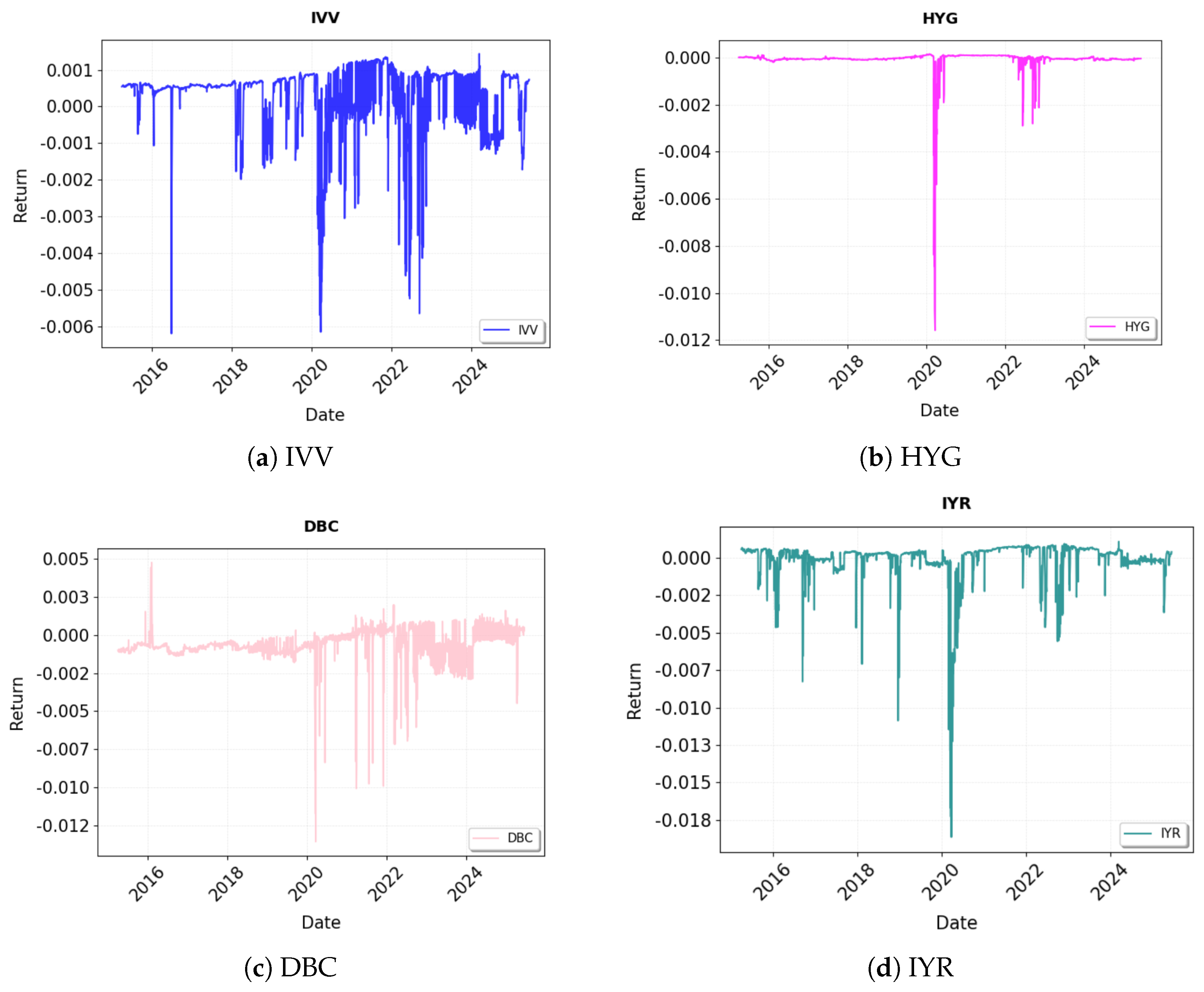
As illustrated in Figure 5, the one-step-ahead rolling expected return forecasts for the four major asset classes—represented by their respective benchmark ETFs—exhibit fluctuating trends, marked by a pronounced downturn in 2020, which is consistent with the market disruption caused by the COVID-19 pandemic, followed by a subsequent recovery. Equities (IVV) and commodities (DBC) show heightened volatility, including intermittent negative shocks, while bonds (HYG) demonstrate greater stability throughout the period. Real estate (IYR) also reflects moderate sensitivity to market shifts. This dynamic adaptability underscores the ability of the rolling JM forecasts framework to adjust return expectations in accordance with identified market regimes, thereby supporting timely portfolio reallocations under varying market conditions.

3.5. MPC Asset Allocation

The MPC objective function (Equation (11)) requires careful calibration of the risk aversion parameter $\gamma$ and the regularization coefficients $\kappa$ and $\rho$. As shown in

Table 7. MPC hyperparameters.

Hyperparameter	Values
$\gamma$	0.01, 0.1, 1, 3, 5, 10
$\kappa$	0.001, 0.005, 0.01, 0.05, 0.1, 0.5, 1, 5
$\rho$	0, 0.0001, 0.0005, 0.001, 0.002

, the candidate values for these hyperparameters are chosen to span a wide and realistic range of possible configurations, following Li et al. [27]. Specifically, different values of $\gamma$ reflect varying degrees of investor risk aversion, allowing us to assess its impact on portfolio optimization outcomes. Meanwhile, $\kappa$ and $\rho$ act as ${\mathsf{\ell }}_1$ regularization hyperparameters, whose selected values help control model complexity, enhance generalization, and mitigate potential overfitting. This comprehensive parameter setup enables a thorough evaluation of the sensitivity of MPC optimization to its key tuning parameters.

Employing a grid search algorithm, we systematically optimized the hyperparameters above by evaluating each candidate combination through the following procedure: first, computing the MPC-derived portfolio weights; second, conducting out-of-sample backtests over the historical data; and finally, selecting the configuration that maximized the portfolio’s Sharpe ratio. The optimal hyperparameter sets identified for each prediction horizon are summarized in

Table 8. MPC hyperparameter tuning results across prediction horizons.

Horizon	$\mathit{\gamma }$	$\mathit{\kappa }$	$\mathit{\rho }$	Sharpe Ratio
H = 1	5	0.001	0.01	0.1347
H = 5	5	0.005	0.001	0.2291
H = 15	5	0.001	0.0005	0.3342
H = 25	5	0.005	0.001	0.2783

. The results indicate that a moderate risk aversion level ($\gamma =5$) remains consistent across all prediction horizons, while the regularization parameters ($\kappa$ and $\rho$) vary to adapt to different forecast conditions. The highest risk-adjusted performance, as measured by the Sharpe ratio, is achieved at the medium-term horizon (H = 15), suggesting an optimal balance between return capture and regularization effectiveness in this setting.

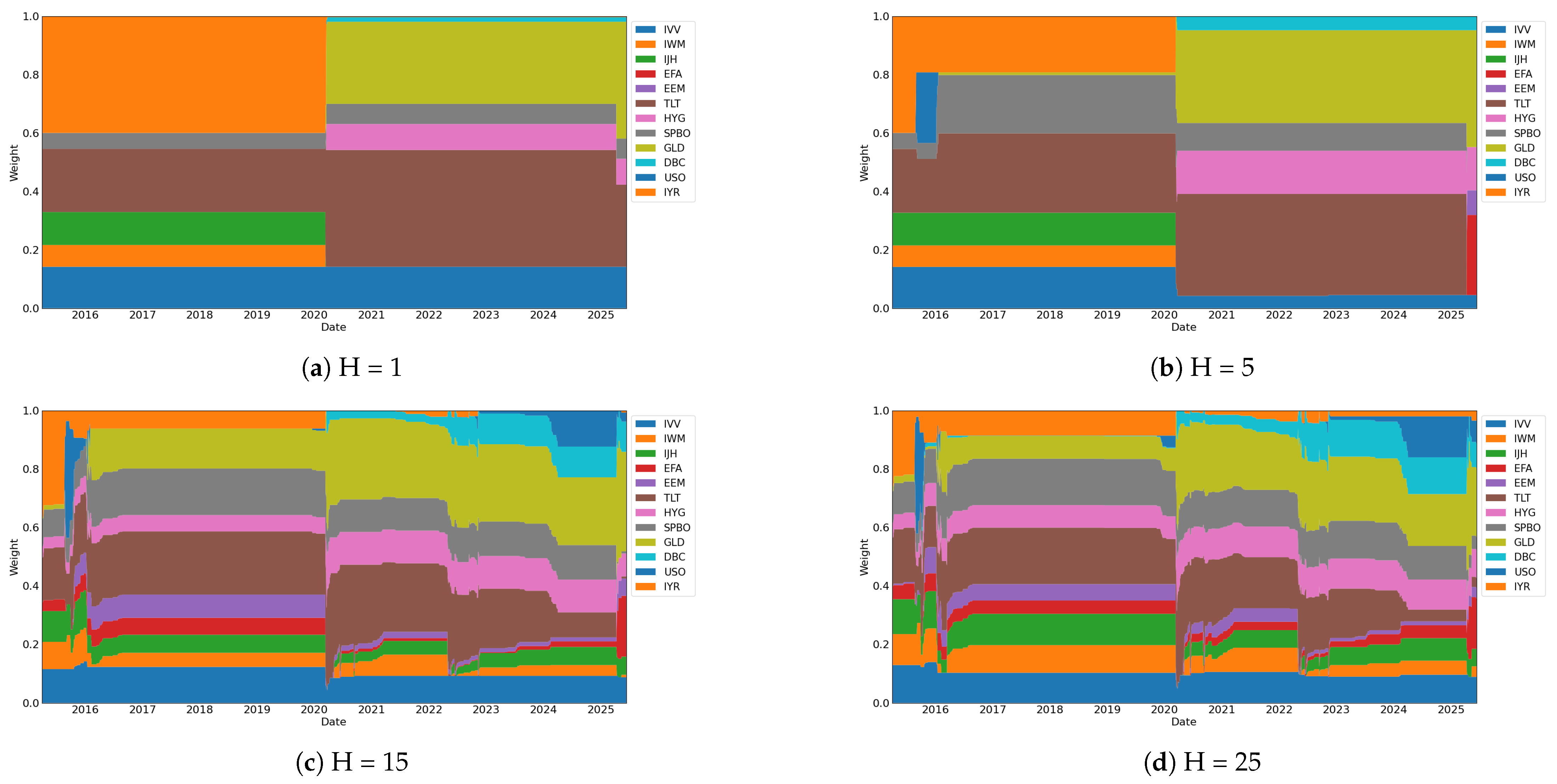
Figure 6 presents the portfolio weights derived from the MPC strategy under different forecasting horizons. Short-term forecasts (H = 1, 5) maintain relatively stable and concentrated allocations, reflecting a tactical response to recent market conditions. In contrast, longer horizons (H = 15, 25) exhibit more frequent rebalancing and greater diversification, emphasizing risk management in uncertain environments. The framework also demonstrates clear adaptation to regime shifts, such as during the 2020 market turmoil, where all horizons reduced exposure to high-risk assets (e.g., IVV, IJH, IWM, and DBC) and increased holdings in defensive instruments (e.g., TLT, HYG, and SPBO). This dynamic reallocation highlights the model’s sensitivity to changing conditions and its economically intuitive optimization mechanism.

3.6. Portfolio Backtest

To evaluate the historical performance of the JM-MPC-optimized portfolio, we conduct a comprehensive backtesting of portfolio returns, with particular focus on market turbulence periods. An equally-weighted portfolio is established as the benchmark for comparison with the JM-MPC portfolio. To simulate real trading conditions, we incorporate transaction cost constraints with a unit cost of 0.1%. The total transaction cost C is given by

$$C=0.01\%\times \sum _{i=1}^n\left|{\tilde{w}}_i\right|$$

(14)

where ${\tilde{w}}_i$ represents the weight adjustment of the i-th asset.

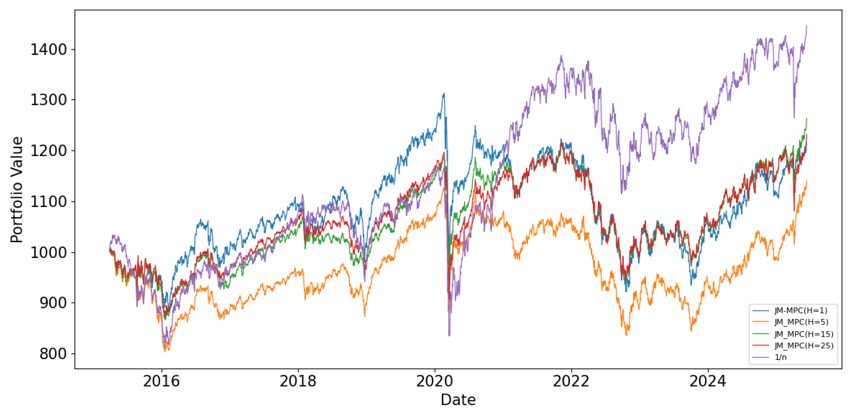
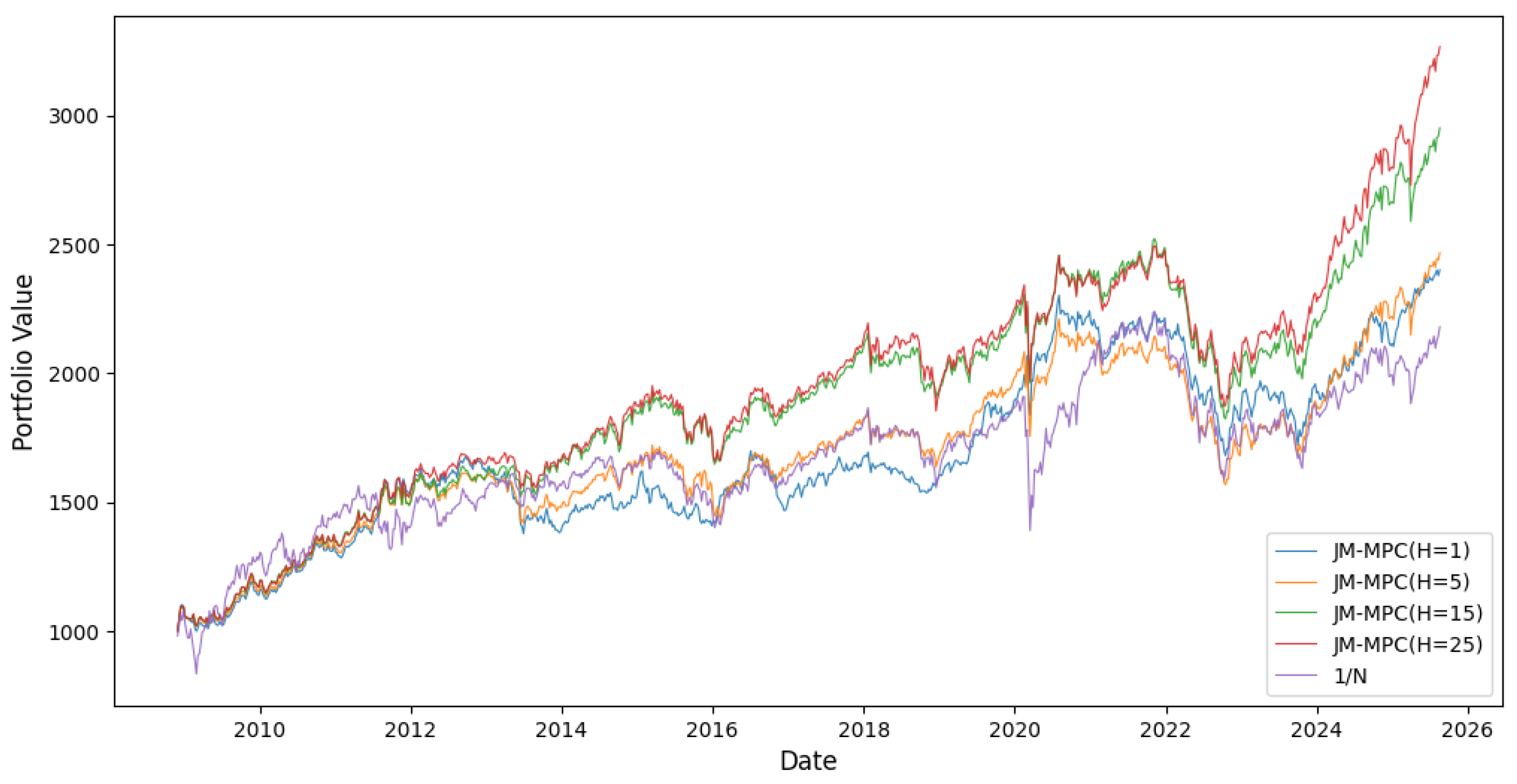
Assuming an initial investment of 1000, Figure 7 shows the value trajectories of different portfolios after transaction costs during the backtesting period. Compared to the equally weighted portfolio (1/N), the JM-MPC-optimized portfolio demonstrates two key advantages: (1) it significantly reduces drawdowns during periods of high market volatility (e.g., the 2008 financial crisis and the 2020 pandemic), and (2) it generates more stable long-term returns. Furthermore, JM-MPC portfolios with different prediction horizons exhibit distinct characteristics—those with shorter horizons show smaller drawdowns during turbulent markets, while medium-to-long-term horizons provide higher returns in low-volatility regimes.

As demonstrated by the portfolio performance metrics in

Table 9. Portfolio performance metrics.

Portfolio Name	Excess Return	Excess Std	Sharpe Ratio	Max Drawdown	Calmar Ratio
JM-MPC (H = 1)	−0.0001	0.1078	−0.0013	0.2975	−0.0005
JM-MPC (H = 5)	−0.0064	0.0962	−0.0661	0.2581	−0.0246
JM-MPC (H = 15)	0.0044	0.0928	0.1446	0.2262	0.0623
JM-MPC (H = 25)	0.0015	0.0971	0.0159	0.2412	0.0064
1/N	0.0178	0.1229	0.0467	0.2858	0.0193

Note: All metrics are annualized indicators calculated based on 252 trading days per year. The bold results indicate the optimal backtesting outcomes for each performance metric.

, the JM-MPC-optimized portfolios exhibit competitive risk-adjusted performance, with the equally weighted portfolio achieving the highest excess return of 0.0178. Notably, the JM-MPC (H = 15) portfolio stands out with the highest Sharpe ratio of 0.1446 and a relatively low max drawdown of 0.2262, highlighting the effectiveness of medium-term JM-MPC optimization in delivering robust risk-adjusted returns. Additionally, the JM-MPC (H = 15) portfolio achieves the highest Calmar ratio of 0.0623, underscoring the superior resilience and return potential of long-term JM-MPC optimization during periods of extreme market volatility.

3.7. Robustness Test

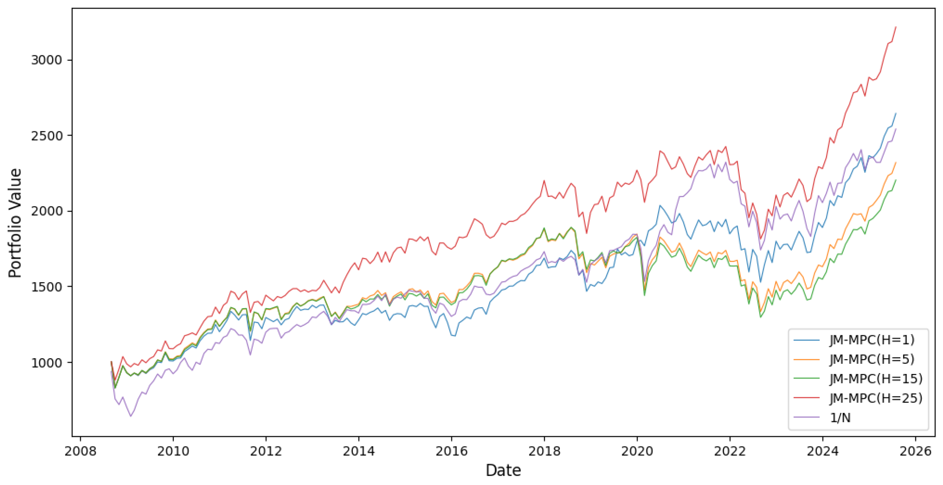
To further evaluate the robustness of the proposed JM-MPC framework, we extend our empirical analysis to weekly and monthly frequencies. Given that weekly and monthly data offer fewer observations compared to daily data, the dataset for these frequencies spans nearly 20 years, from 2005 to 2025. Rolling window sizes are set to 150 and 36 for weekly and monthly frequencies, respectively, corresponding to approximately three years of data in each window. The empirical investigation follows the same JM-MPC framework as described above. All hyperparameters remain unchanged from the daily frequency analysis to ensure consistency in the backtesting procedure.

As shown in Figure 8 and Figure 9, JM-MPC strategies with longer prediction horizons (H = 15 and H = 25) consistently outperform the equally weighted (1/N) benchmark in reducing portfolio drawdowns. This advantage is particularly evident during periods of high market volatility, such as the 2008 financial crisis and the 2020 market turbulence. Furthermore, both weekly and monthly rebalancing frequencies achieve higher cumulative returns compared to daily rebalancing. This performance improvement may be attributed to the smoother nature of lower-frequency data, which provides a more stable capture of underlying market trends and thereby supports more robust asset allocation decisions.

Table 10. Portfolio performance metrics.

Data Frequency	Portfolio Name	Sharpe Ratio	Max Drawdown	Calmar Ratio
Weekly	JM-MPC (H = 1)	0.5445	0.2702	0.1981
	JM-MPC (H = 5)	0.5381	0.2909	0.1898
	JM-MPC (H = 15)	0.6396	0.2769	0.2404
	JM-MPC (H = 25)	0.6971	0.2490	0.2933
	1/N	0.3460	0.2912	0.1671
Monthly	JM-MPC (H = 1)	0.4459	0.2430	0.2353
	JM-MPC (H = 5)	0.3852	0.2942	0.1723
	JM-MPC (H = 15)	0.3591	0.3154	0.1507
	JM-MPC (H = 25)	0.6091	0.2524	0.2817
	1/N	0.4378	0.3174	0.1907

Note: All metrics are annualized indicators. Weekly and monthly metrics are calculated based on 52 weeks and 12 months per year, respectively. The bold results indicate the optimal backtesting outcomes for each performance metric.

presents the performance metrics from weekly and monthly backtests. Among all strategies, JM-MPC (H = 25) achieves the highest Sharpe and Calmar ratios, as well as the smallest maximum drawdown under both rebalancing frequencies—demonstrating superior long-term risk-adjusted performance and resilience. These results confirm the stability and adaptability of our JM-MPC framework in different data frequencies.

3.8. Economic Interpretation of the Empirical Results

In this section, we explain how our empirical results demonstrate strong economic rationality across three key dimensions. The superior performance of the proposed JM-MPC framework can be attributed to its ability to capture fundamental market mechanisms and incorporate them into the portfolio optimization process.

First, the superior performance of our JM-MPC framework relative to the static equal-weighted benchmark is economically intuitive. It arises from the JM’s capacity to identify and dynamically adapt to distinct market regimes (see Figure 4). This behavior mirrors the flight-to-quality phenomenon observed in real markets, in which capital shifts from risky to safe assets during periods of turbulence [4].

Second, robustness analysis demonstrates that the enhanced performance under weekly and monthly frequencies—compared to daily rebalancing—stems from the low signal-to-noise ratio inherent in high-frequency financial data [33]. Lower-frequency data effectively filter out transient noise and microstructure effects, thereby capturing persistent macroeconomic trends and fundamental drivers of long-term asset prices more reliably.

Finally, the improved outcomes at medium- and long-term forecast horizons (H = 15, H = 25) underscore the value of a forward-looking, strategic perspective. Longer prediction horizons mitigate overreaction to short-term fluctuations and allow the model to incorporate slower-moving business cycle information, resulting in more stable and economically better-founded portfolio allocations.

4. Conclusions

We propose a novel framework (JM-MPC) that integrates the jump model (JM) with model predictive control (MPC) for regime-dependent multi-period portfolio optimization. The JM generates rolling predictions of expected returns and covariance matrices by explicitly capturing regime-switching dynamics; MPC utilizes multi-horizon JM forecasts as inputs to solve sequential portfolio rebalancing problems. Key findings are as follows:

Hyperparameter and feature selection results demonstrate that the SJM framework effectively captures both universal market characteristics and asset-specific dynamics through two key findings: (1) all assets share common optimal hyperparameters ($\lambda =100$, $\kappa =5$) for regime transitions while exhibiting risk-dependent state dimensionality (K = 2 for bonds vs. 3–4 for equities/commodities); (2) feature importance analysis confirms this dichotomy, with sentiment indicators dominating risky assets and fundamental factors governing defensive assets. Furthermore, the rolling forecasts demonstrate that the JM can effectively incorporate market regime information to generate multi-horizon predictions of both expected returns and return covariance matrices. Crucially, the predicted expected returns show economically plausible alignment with observed market fluctuations, validating the model’s dynamic adaptability.

Empirical results affirm the effectiveness of the JM-MPC framework in enhancing portfolio performance, particularly during high-volatility market regimes such as the 2008 financial crisis and the COVID-19 pandemic. The framework significantly reduces drawdowns and improves overall returns by dynamically adapting to identified market regime information. Furthermore, MPC optimization demonstrates horizon-dependent performance, with medium-to-long-term prediction horizons (H = 15, =25) consistently outperforming short-term forecasts (H = 1, H = 5). Robustness analysis further demonstrates consistent superiority under weekly and monthly rebalancing compared to daily frequency, confirming the stability of its performance across different data frequencies and investment horizons. Economically, these findings highlight the ability of JM-MPC to leverage regime-sensitive, multi-horizon forecasts for robust asset allocation, translating market insights into resilient portfolio strategies under uncertainty.

The JM-MPC framework demonstrates promising performance in dynamic asset allocation, yet it faces three main limitations: First, its sensitivity to parameter selection considerably influences both regime identification and portfolio optimization results. Future studies could adopt adaptive hyperparameter tuning methods—such as Bayesian optimization—to improve regime detection robustness. Second, although this study uses a centralized optimization approach, emerging distributed resource allocation algorithms [34] suggest alternative architectures. Future work may develop distributed JM-MPC variants that decompose portfolio optimization across multiple agents or assets, improving computational efficiency for large-scale portfolios via consensus mechanisms. Third, while the jump model captures regime-switching dynamics, it omits finer stochastic properties of return distributions—especially higher-order moments and tail behaviors. Subsequent research could integrate advanced stochastic techniques, such as Lévy processes or stochastic volatility models, to better represent financial returns’ complex stochastic nature and strengthen economic realism.

References

1. Branch, W.A.; Evans, G.W. Asset return dynamics and learning. Rev. Financ. Stud. 2010, 23, 1651–1680. [Google Scholar] [CrossRef]
2. Ang, A.; Bekaert, G. How regimes affect asset allocation. Financ. Anal. J. 2004, 60, 86–99. [Google Scholar] [CrossRef]
3. Hu, S.; Zhang, W.; Li, D.; Wu, B. Incorporating improved directional change and regime change detection to formulate trading strategies in foreign exchange markets. Phys. A Stat. Mech. Its Appl. 2023, 622, 128810. [Google Scholar] [CrossRef]
4. Shu, Y.; Yu, C.; Mulvey, J.M. Downside risk reduction using regime-switching signals: A statistical jump model approach. J. Asset Manag. 2024, 25, 493–507. [Google Scholar] [CrossRef]
5. Baum, L.E.; Petrie, T. Statistical inference for probabilistic functions of finite state Markov chains. Ann. Math. Stat. 1966, 37, 1554–1563. [Google Scholar] [CrossRef]
6. Hamilton, J.D. Analysis of time series subject to changes in regime. J. Econom. 1990, 45, 39–70. [Google Scholar] [CrossRef]
7. Bulla, J. Hidden Markov models with t components. Increased persistence and other aspects. Quant. Financ. 2011, 11, 459–475. [Google Scholar] [CrossRef]
8. Wang, M.; Lin, Y.-H.; Mikhelson, I. Regime-switching factor investing with hidden Markov models. J. Risk Financ. Manag. 2020, 13, 311. [Google Scholar] [CrossRef]
9. Maruotti, A.; Punzo, A.; Bagnato, L. Hidden Markov and semi-Markov models with multivariate leptokurtic-normal components for robust modeling of daily returns series. J. Financ. Econom. 2019, 17, 91–117. [Google Scholar] [CrossRef]
10. Zheng, K.; Li, Y.; Xu, W. Regime switching model estimation: Spectral clustering hidden Markov model. Ann. Oper. Res. 2021, 303, 297–319. [Google Scholar] [CrossRef]
11. Bemporad, A.; Breschi, V.; Piga, D.; Boyd, S.P. Fitting jump models. Automatica 2018, 96, 11–21. [Google Scholar] [CrossRef]
12. Kim, M.J.; Kwon, D. Dynamic asset allocation strategy: An economic regime approach. J. Asset Manag. 2023, 24, 136–147. [Google Scholar] [CrossRef]
13. Mc Greevy, J.; Muguruza, A.; Issa, Z.; Salvi, C.; Chan, J.; Zuric, Z. Detecting Multivariate Market Regimes via Clustering Algorithms. Available online: https://papers.ssrn.com/sol3/papers.cfm?abstract_id=4758243 (accessed on 30 August 2025).
14. Antulov-Fantulin, N.; Cauderan, A.; Kolm, P.N. A Dynamic Regime-Switching Model Using Gated Recurrent Straight-Through Units. J. Financ. Data Sci. 2024, 6, 4. [Google Scholar]
15. Tan, Z.; Wu, Y. On regime switching models. Mathematics 2025, 13, 1128. [Google Scholar] [CrossRef]
16. Tu, J. Is regime switching in stock returns important in portfolio decisions? Manag. Sci. 2010, 56, 1198–1215. [Google Scholar] [CrossRef]
17. Nystrup, P. Dynamic Asset Allocation—Identifying Regime Shifts in Financial Time Series to Build Robust Portfolios. Ph.D. Thesis, DTU Compute, Kongens Lyngby, Denmark, 2018. [Google Scholar]
18. Costa, G.; Kwon, R.H. Risk parity portfolio optimization under a Markov regime-switching framework. Quant. Financ. 2019, 19, 453–471. [Google Scholar] [CrossRef]
19. Oprisor, R.; Kwon, R. Multi-period portfolio optimization with investor views under regime switching. J. Risk Financ. Manag. 2020, 14, 3. [Google Scholar] [CrossRef]
20. Black, F.; Litterman, R. Global portfolio optimization. Financ. Anal. J. 1992, 48, 28–43. [Google Scholar] [CrossRef]
21. Shu, Y.; Yu, C.; Mulvey, J.M. Dynamic asset allocation with asset-specific regime forecasts. Ann. Oper. Res. 2024, 346, 285–318. [Google Scholar] [CrossRef]
22. Nystrup, P.; Lindström, E.; Madsen, H. Learning hidden Markov models with persistent states by penalizing jumps. Expert Syst. Appl. 2020, 150, 113307. [Google Scholar] [CrossRef]
23. Nystrup, P.; Kolm, P.N.; Lindström, E. Feature selection in jump models. Expert Syst. Appl. 2021, 184, 115558. [Google Scholar] [CrossRef]
24. Witten, D.M.; Tibshirani, R. A framework for feature selection in clustering. J. Am. Stat. Assoc. 2010, 105, 713–726. [Google Scholar] [CrossRef]
25. Herzog, F.; Dondi, G.; Geering, H.P. Stochastic model predictive control and portfolio optimization. Int. J. Theor. Appl. Financ. 2007, 10, 203–233. [Google Scholar] [CrossRef]
26. Boyd, S.; Busseti, E.; Diamond, S.; Kahn, R.N.; Koh, K.; Nystrup, P.; Speth, J. Multi-period trading via convex optimization. Found. Trends® Optim. 2017, 3, 1–76. [Google Scholar] [CrossRef]
27. Li, X.; Uysal, A.S.; Mulvey, J.M. Multi-period portfolio optimization using model predictive control with mean-variance and risk parity frameworks. Eur. J. Oper. Res. 2022, 299, 1158–1176. [Google Scholar] [CrossRef]
28. Markowitz, H. Portfolio selection. J. Financ. 1952, 7, 77–91. [Google Scholar]
29. Cortese, F.P.; Kolm, P.N.; Lindstrom, E. Generalized Information Criteria for High-Dimensional Sparse Statistical Jump Models. Available online: https://papers.ssrn.com/sol3/papers.cfm?abstract_id=4774429 (accessed on 30 August 2025).
30. Boyd, S.; Mueller, M.T.; O’Donoghue, B.; Wang, Y. others Performance bounds and suboptimal policies for multi–period investment. Found. Trends® Optim. 2013, 1, 1–72. [Google Scholar]
31. Selig, E.; Bilokon, P. Regularised Jump Models for Regime Identification and Feature Selection. Available online: https://papers.ssrn.com/sol3/papers.cfm?abstract_id=4950423 (accessed on 30 August 2025).
32. Aydınhan, A.O.; Kolm, P.N.; Mulvey, J.M.; Shu, Y. Identifying patterns in financial markets: Extending the statistical jump model for regime identification. Ann. Oper. Res. 2024, 1–37. [Google Scholar] [CrossRef]
33. Zhang, L.; Hua, L. Major issues in high-frequency financial data analysis: A survey of solutions. Mathematics 2025, 13, 347. [Google Scholar] [CrossRef]
34. Doostmohammadian, M.; Aghasi, A.; Pirani, M.; Nekouei, E.; Zarrabi, H.; Keypour, R.; Rikos, A.I.; Johansson, K.H. Survey of distributed algorithms for resource allocation over multi-agent systems. Annu. Rev. Control 2025, 59, 100983. [Google Scholar] [CrossRef]
Figure 1. Asset cumulative return over time.
Mathematics 13 02837 g001
Figure 2. Historical closing prices of U.S. Treasury yields and the VIX index.
Mathematics 13 02837 g002
Figure 3. Asset feature weight.
Mathematics 13 02837 g003
Figure 4. Regime classification result of Asset IVV.
Mathematics 13 02837 g004
Figure 5. Expected return based on the 1-step rolling forecast.
Mathematics 13 02837 g005
Figure 6. Asset allocation under the JM-MPC framework with varying prediction horizons.
Mathematics 13 02837 g006
Figure 7. Daily backtested performance of comparative portfolios.
Mathematics 13 02837 g007
Figure 8. Weekly backtested performance of comparative portfolios.
Mathematics 13 02837 g008
Figure 9. Monthly backtested performance of comparative portfolios.
Mathematics 13 02837 g009