Design of Intelligent Control Using Dynamic Petri, CMAC, and BCMO for Nonlinear Systems with Uncertainties

Abstract

This paper presents a novel dynamic Petri fuzzy neural network (DPFNN) for controlling the position of a metal ball in a magnetic levitation system (MLS). The DPFNN reduces parameter learning costs by combining Petri nets and fuzzy frameworks. Given the nonlinear and uncertain dynamics of the MLS, an adaptive DPFNN control system was developed for high-precision position control. The parameter set has been optimized using the BCMO algorithm for the best performance. The desired system stability and control performance can be achieved by the proposed control system.

1. Introduction

Magnetic levitation is a technology that uses magnetic fields to suspend objects in the air without physical contact. By counteracting gravity through electromagnetic forces, this creates a frictionless environment, allowing for smooth and efficient movement [1]. This technology not only promises to redefine high-speed travel but also extends its utility to diverse applications, from precision manufacturing to energy harvesting. Due to continuous progress in industrial technology, magnetic levitation systems (MLS) have become increasingly prevalent, particularly in high-precision positioning tasks [2]. The choice of an effective yet uncomplicated control approach continues to pose a major challenge in MLS advancement, positioning research into these systems as a leading focus in the field.

In recent years, numerous studies have sought to improve MLS performance. In 2020, Wang et al. presented an adaptive terminal sliding mode control approach with improved disturbance rejection [3]. In 2021, Vo et al. developed a fixed-time trajectory tracking controller for uncertain MLS [4]. Zhang et al. designed and implemented a Takagi–Sugeno fuzzy controller for a magnetic levitation ball [5]. Despite their effectiveness, these methods often involve complex computational processes, and there remains room for enhancing control performance. Meanwhile, fuzzy neural networks (FNNs) have several advantages, including fast learning speed, simple realization, and dealing with nonlinear systems. To solve the above problems in terms of better performance and simpler computation, a dynamic Petri fuzzy neural network (DPFNN) is developed in this study to achieve precise control of nonlinear MLS.

Given the substantial complexity and nonlinear dynamics of MLS, traditional model-based control strategies are often unsuitable for its regulation. As a result, model-free control approaches have been deemed more appropriate for such systems. In particular, neural networks (NNs) have attracted significant attention across various fields [6,7,8,9,10,11]. While NNs possess universal approximation capability for continuous functions, their learning process is global, requiring updates to all weights during each training iteration, which results in comparatively slow convergence. Furthermore, in fully connected NNs, approximation performance strongly depends on the quality and comprehensiveness of the training dataset, restricting their effectiveness in online learning applications. To counter these limitations, fuzzy neural networks (FNNs) appear to be a promising alternative. FNNs integrate the adaptive learning ability of neural networks with the linguistic reasoning and interpretability of fuzzy logic. FNNs offer lower computational complexity and faster learning speed while retaining the capability for efficient knowledge representation and inference.

Petri nets (PN) are a mathematical modeling language used to describe and analyze systems where concurrent, asynchronous, distributed, or parallel behaviors occur, particularly in computer science, manufacturing, workflows, and biological processes [12]. Dynamic Petri (DP) extends the basic Petri net framework to model systems with dynamic behavior, such as those with variable structure, evolving state spaces, or changing topology. These models allow for the representation of systems in which transitions between states may depend on conditions that evolve over time [13]. DP approaches have been utilized across multiple domains, including computer networks, manufacturing systems, workflow management, and biological systems [14,15,16,17,18,19]. Li et al. (2019) created an improved FMEA framework by integrating interval type-2 fuzzy sets with fuzzy Petri nets, thereby overcoming the shortcomings of the conventional RPN approach and enhancing the dependability of risk assessment in aerospace electronics production [20]. Then, in 2020, Hu and Liang suggested a dynamic scheduling approach for flexible manufacturing systems using Petri nets and deep reinforcement learning combined with graph convolutional networks [21]. More recently, Wang et al. (2022) developed a fuzzy Petri net model that integrates the synergistic effects of events, leading to improved reasoning abilities in knowledge-based systems [22].

In this study, we propose a novel approach that integrates the dynamic Petri fuzzy neural network (DPFNN) with balanced composite motion optimization (BCMO) [23,24] for the control of nonlinear systems and chaotic synchronization [25,26,27,28,29,30]. The adoption of a multilayer framework strengthens both the learning capacity and adaptability of the DP mechanism. Unlike conventional designs, the proposed DP-based TSKCMAC architecture provides several distinct benefits. Its hierarchical structure improves generalization and reduces the number of fuzzy rules by efficiently covering the input space, thereby increasing computational efficiency. Moreover, embedding DP as an intermediate layer within TSKCMAC enables dynamic token generation and adaptive fuzzy rule selection according to the activated nodes, which enhances decision-making in complex environments. An additional advantage of the DP functionality is its ability to improve system robustness while simultaneously eliminating redundant fuzzy rules, resulting in a compact and effective rule base and further boosting overall system performance. Although the proposed method adopts a hybrid architecture consisting of a Petri net supervisor, a fuzzy CMAC controller, and a BCMO optimizer, it is specifically designed so that most computational effort is shifted to the offline phase. Compared to existing methods [3,4] that require iterative optimization or reinforcement learning computations during online execution, the online implementation of the proposed system only involves a Petri net-driven switching logic and a CMAC table lookup. These operations are of constant-time complexity have no need for real-time policy search or gradient-based adaptation. Therefore, in practice our approach achieves fast and lightweight online execution by reducing computational complexity, which is detailed in Section 3.

This paper has been successfully employed in two test cases: a metal ball controlled in a magnetic levitation system [31,32,33], and a mass–spring–damper setup [34]. The proposed DPCMAC controller is constructed to avoid heavy computational demand while retaining the inherent benefits of the CMAC framework, which reduces the processing load associated with parameter learning. Furthermore, it is equipped with mechanisms to effectively compensate for approximation errors [35,36,37,38]. Based on adaptive tuning principles, optimal control performance can be attained by adjusting the control parameters. Additionally, the developed intelligent controller is executed using a field-programmable gate array (FPGA) chip [39], which enables compact design, cost efficiency, high execution speed, and enhanced flexibility [40]. The results from both the simulation and experiments of the magnetic levitation system have been provided to demonstrate the outstanding control capabilities of the proposed intelligent controller

2. Magnetic Levitation System Description

2.1. Modeling of Magnetic Levitation System

For the uniaxial magnetic levitation system presented in Figure 1, a voltage input is converted into current through a driver circuit, which excites the electromagnet, generating a magnetic field that affects its vicinity. The metallic ball within this region undergoes a magnetic force along the vertical axis of the electromagnet, enabling it to levitate. Meanwhile, an infrared sensor keeps track of the ball’s position and provides feedback to the control system to ensure stability. The dynamics of the ball can be demonstrated by Newton’s second law, which can be expressed as follows:

$$Ma=F(x,I)-M{g}_m$$

(1)

where M denotes the mass of the levitated ball, $g_m$ is the gravitational acceleration, x represents the vertical displacement of the ball relative to the electromagnet, and $F(x,I)$ corresponds to the magnetic control force.

The magnetic control force of the MLS as a function of displacement x and current I can be formulated as follows:

$$\begin{array}{c}F(x,I)={\displaystyle \frac{{\mu }_0{N}^4{I}^{2}S}{8}}\left((x+h)ln\left|{\displaystyle \frac{R_2+\sqrt{R_2^2+{(x+h)}^2}}{R_1+\sqrt{R_1^2+{(x+h)}^2}}}\right|{\left.+xln\left|{\displaystyle \frac{R_1+\sqrt{R_1^2+x^2}}{R_2+\sqrt{R_2^2+x^2}}}\right|\right)}^2\right.\hfill \\ \hfill \end{array}$$

(2)

where ${\mu }_0$ represents the permeability of free space, h represents the coil’s length, N represents the number of turns per meter, S represents the material surface that the magnetic flux crosses, $R_1$ represents the lowest coil radius, and $R_2$ represents the maximum coil radius.

It should be noted that the magnetic field exerts opposite effects on the sphere; as illustrated in Figure 2, an attractive force is emitted at the North pole, while a contrasting repulsive force is generated at the South pole. Consequently, the resulting magnetic force acting on the ball, denoted by $g(x,l)$, can be expressed as

$$g(x,I)=F(x,I)-F(x+\delta x,I),$$

(3)

where $F(x,I)$ is the attractive force on the North pole and $F(x+\delta x,I)$ is the repulsive force on the South pole.

It is important to note that Equations (1) and (2) represent the dynamics of the system, and are used for simulation only. The effect on the system models of practically implementing the proposed controller is negligible.

2.2. Ideal Backstepping Controller (IBC)

Step 1: Determine the tracking error

$$e_1=x_d-x$$

(4)

and specify the stabilizing function

$$\alpha =a_1{e}_1+{\dot{x}}_d,$$

(5)

where ${\alpha }_1$ is a positive constant. In addition, define

$$e_2=\alpha -\ddot{x}={\dot{e}}_1+a_1{e}_1.$$

(6)

Then, $e_2$ can be derived to

$$\begin{array}{c}{\dot{e}}_2=\dot{\alpha }-\ddot{x},\hfill \\ =\dot{\alpha }-\left[f\left(x\right)+u+\mathrm{\Delta }f\left(x\right)+d\left(x\right)\right],\hfill \\ ={\ddot{e}}_1+a_1{\dot{e}}_1.\hfill \end{array}$$

(7)

Step 2: Define the following Lyapunov function:

$$V_1={\displaystyle \frac{1}{2}}{e}_1^2+{\displaystyle \frac{1}{2}}{e}_2^2.$$

(8)

Then, $V_1$ can be derived to

$$\begin{array}{c}{\dot{V}}_1=e_1{\dot{e}}_1+e_2{\dot{e}}_2,\hfill \\ =-a_1{e}_1^2+e_2{e}_1+e_2{\dot{e}}_2,\hfill \\ =-a_1{e}_1^2+e_2\left[e_1+\dot{\alpha }-f\left(x\right)\right.\left.-u-\mathrm{\Delta }f\left(x\right)-d\left(x\right)\right].\hfill \end{array}$$

(9)

Step 3: Assume that the dynamic models ($f_0\left(\mathbf{x}\right),g_0$, and $d_0\left(\mathbf{x}\right)$) are precisely recognized; then, the IBC can be stated as

$$u_{IBC}^{*}={\displaystyle \frac{1}{g_0}}\left(\dot{\alpha }-f_0\left(\mathbf{x}\right)-d_0\left(\mathbf{x}\right)+e_1+a_2{e}_2\right),$$

(10)

where $a_2$ is a positive constant. By substituting (10) into (9), the system dynamics can be reformulated as

$${\dot{V}}_1=-a_1{e}_1^2-a_2{e}_2^2\le 0,$$

(11)

guaranteeing the stability of the IBC system.

3. Intelligent Control System Design

3.1. Petri Net

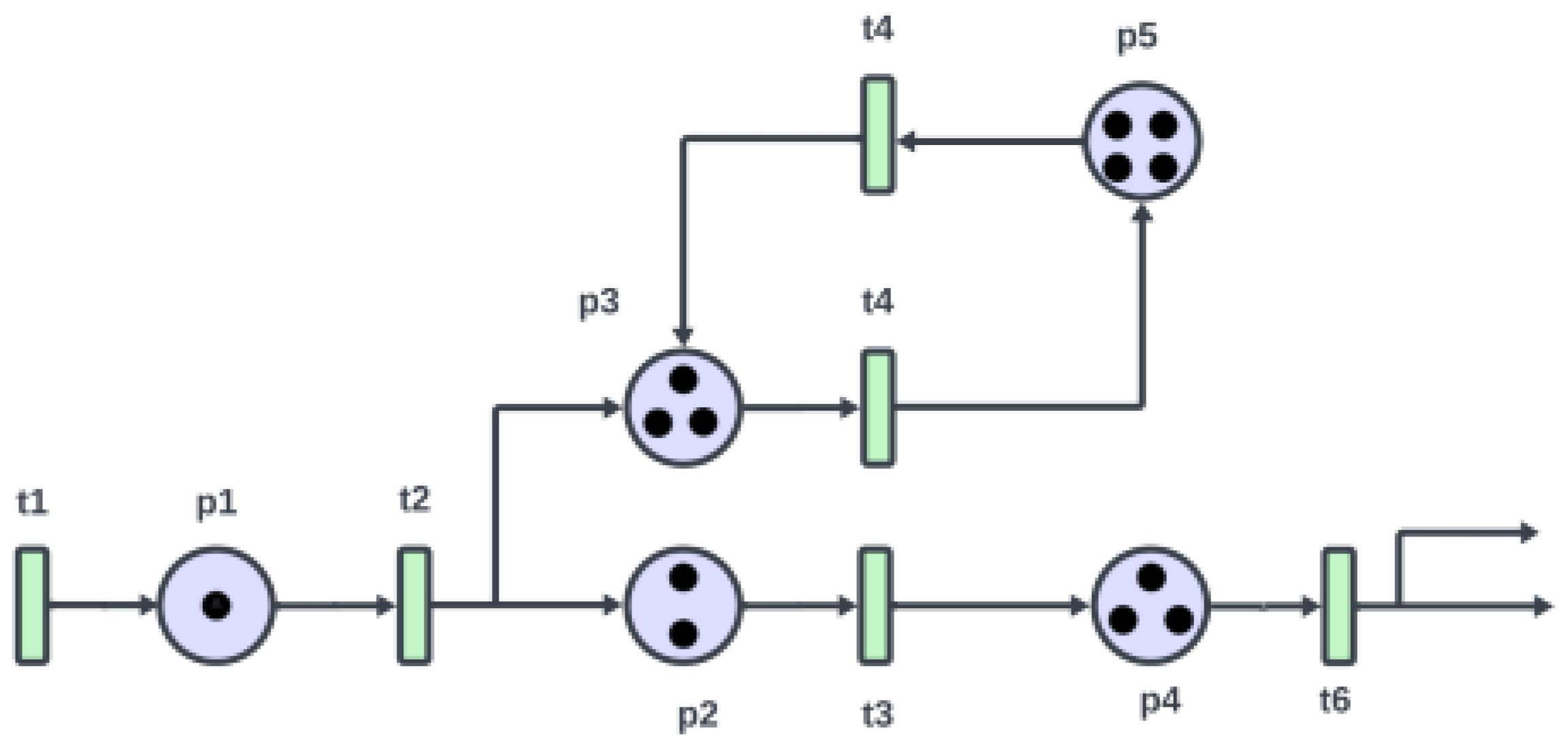
A directed bipartite network containing two different node types (referred to as “places” and “transitions”) is called a Petri net (PN). Directed arcs never connect two locations or two transitions; instead, they only connect certain locations and positions with exits. The transitions and locations are represented by rectangles and circles, respectively. One or more tokens may be represented by dots in each location. The system’s behavior is modeled thanks to these tokens. A vector containing positive integer values makes up a PN’s marking. The $n^{th}$ component of this vector is equal to the number of tokens in the place numbered n in the Petri net, and its dimension is equal to the number of places [13].

Consideration of the PN represented in Figure 3 illustrates the definition above. This PN contains five places and six transitions, denoted by $p_1,p_2,p_3,p_4,p_5$ and $t_1,t_2,t_3,t_4,t_5,t_6$, respectively. Formally, the structure of a PN can be described as

$$\psi =\left(S_P,S_T,M_I,M_O,A\right),$$

(12)

where $S_P=\left(p_1,p_2·····p_m\right)$ is a set of places and $S_T=\left(t_1,t_2·····t_n\right)$ is a set of transitions. Given that both $S_P$ and $S_T$ are finite, $M_I:S_P\times S_T\to \left\{0,1\right\}$ is a mapping between places and transitions, also known as the input function. In detail, $M_I\left(p_i,t_j\right)=1$ if there is a directed arc from $p_i$ to $t_j$, while $M_I\left(p_i,t_j\right)=0$ if there are no directed arcs from $p_i$ to $t_j$ with i in the range of 1 to m and j is in the range of 1 to n. Finally, $M_O:S_P\times S_T\to \left\{0,1\right\}$ is a mapping from transitions to places, also known as the output function.

Similarly to $M_I$, if there is a directed arc from $t_j$ to $p_i$, then $M_O\left(p_i,t_j\right)=1$; otherwise, $M_O\left(p_i,t_j\right)=0$, with i in the range of 1 to m and j in the range of 1 to n. Here, $A:S_P\to \left[0,1\right]$ is a mapping from places to real values between zero and one, which is called an association function.

According to the transition (firing) rule, a state or marking in a PN must be changed in order to replicate the dynamic behavior of real-world systems [22].

(1)

If a transition $t_j$ has input places $p_i$ that are marked as tokens, then $t_j$ is enabled.

(2)

Depending on whether the event takes place, an enabled transition might or might not activate.

(3)

One token is added to each output location, and the tokens from each input site are deleted when an enabled transition is triggered.

In a normal PN, a site accumulates tokens and initiates the output transition if the quantity of tokens exceeds a threshold value.

3.2. Fuzzy Neural Network

The fuzzy inference rules for the novel fuzzy neural network (FNN) depicted in Figure 4 are described below.

If $I_1$ is $F_{1jk}$, $I_2$ is $F_{2jk}$,…, and $I_{n_i}$ is $F_{n_{i}jk}$, then $R^l$ provides the following statement.

The output is defined as $o_{jk}=w_{jk}$, where $j=1,\dots ,n_j$, $k=1,\dots ,n_k$, and $l=1,\dots ,n_l$. Here, $n_i$ denotes the input dimension, $n_j$ represents the number of layers assigned to each input dimension, $n_k$ is the number of blocks within a layer, and $n_l$ corresponds to the total number of fuzzy rules. The set $F_{ijk}$ specifies the fuzzy region associated with the $i^{\mathrm{th}}$ input, $j^{\mathrm{th}}$ layer, and $k^{\mathrm{th}}$ block, while $w_{jk}$ is the singleton weight in the resulting part. In contrast to traditional fuzzy neural networks, the fuzzy CMAC uses an input space that is divided into layers and blocks. Furthermore, the fuzzy CMAC reduces to a typical fuzzy neural network in which each block has a single element (neuron) and each input dimension has a single layer. As a result, this fuzzy CMAC can be thought of as a generalization of a fuzzy neural network, and outperforms fuzzy neural networks in terms of generalization, learning features, and recall.

The input, association memory, receptive field, weight memory, and output are the five primary parts of the fuzzy CMAC architecture. Below, we provide a description of how signals travel via these parts.

(1)

Input: Each input state variable $I_i$ can be quantized into distinct regions (referred to as elements or neurons) using the provided control space and a specified set of inputs $I={[I_1,I_2,\cdots ,I_{n_i}]}^T\in {\Re }^{n_i}$. The resolution is determined by the number of elements $n_e$.

(2)

The association memory, also referred to as the membership function, involves assembling several components into a logical whole. Every single block serves as a receptive field basis inside this specified domain. The type-2 wavelet function is the receptive field basis function employed in this investigation, which has the following mathematical expression:

$$F_{ijk}\left(f_{ijk}\right)=-{\displaystyle \frac{f_{ijk}}{2}}exp(-f_{ijk}^2)$$

(13)

for $i,j,k$ from 1 to $n_i,n_j,n_k$, respectively. In the above equation, $f_{ijk}={\displaystyle \frac{I_i-{\mu }_{ijk}}{{\sigma }_{ijk}}}$, ${\mu }_{ijk}$ is the mean parameter, and ${\sigma }_{ijk}$ is the variance parameter.

(3)

Receptive Field: Each block contains two movable parameters, variance $\sigma$ and mean $\mu$. The multi-dimensional receptive field function is expressed as follows:

$$r_{jk}=\prod _{i=1}^{n_i}{F}_{ijk}\left(f_{ijk}\right)=\prod _{i=1}^{n_i}exp\left(-{({\displaystyle \frac{I_i-{\mu }_{ijk}}{{\sigma }_{ijk}}})}^2\right)$$

(14)

for $j=1,2,\dots ,n_j$ and $k=1,2,\dots ,n_k$, where $r_{jk}$ is indicated with the $j^{th}$ layer and $k^{th}$ block, that is, the product is used as the “and” computation in the antecedent section of the fuzzy rules in (X).

Multi-dimensional receptive field functions can be expressed in vector form as follows:

$$\begin{array}{c}\mathbf{r}={[r_{11},\cdots ,r_{1n_k},r_{21},\cdots ,r_{2n_k},\cdots ,r_{n_{j}1},\cdots ,r_{n_j{n}_k}]}^T\in {\Re }^{n_j{n}_k}\hfill \\ ={[r_1,\cdots ,r_l,\cdots ,r_{n_l}]}^T\in {\Re }^{n_l}.\hfill \end{array}$$

(15)

(4)

Weight Memory: Each position of the receptive field with respect to a specific adjustable value in the weight memory space can be expressed as follows:

$$\begin{array}{c}\mathbf{w}={[w_{11},\cdots ,w_{1n_k},w_{21},\cdots ,w_{2n_k},\cdots ,w_{n_{j}1},\cdots ,w_{n_j{n}_k}]}^T\in {\Re }^{n_j{n}_k}\hfill \\ \hfill \\ ={[w_1,w_2,\cdots ,w_{n_l}]}^T\in {\Re }^{n_l}\hfill \end{array}$$

(16)

where $w_{j}k$ indicates the connecting weight value of the output linked with the $j^{th}$ layer and $k^{th}$ block.

(5)

Output: The algebraic sum of the activated weighted receptive field indicates the output of fuzzy CMAC, with has the following representation:

$$U_{FCMAC}=O={\mathit{w}}^T\mathit{r}=\sum _{j=1}^{n_j}\sum _{k=1}^{n_k}{w}_{jk}{r}_{jk}=\sum _{l=1}^{n_l}{w}_l{r}_l$$

(17)

that is, Equation (17) represents the defuzzification of the fuzzy system in (13). The fuzzy CMAC can be regarded as a generalized framework. When restricted to a single layer with each block containing only one element, the structure degenerates into a conventional fuzzy rule-based system [21]. Under the same condition, the wavelet fuzzy CMAC likewise simplifies to a wavelet neural network [17,18,19]. Furthermore, it simplifies to a fuzzy neural network [11] if the wavelet mother function is removed, and can be simplified to a traditional CMAC [14,15,16] if the fuzzy rules and wavelet mother function are removed.

3.3. Architecture of a Recurrent Petri Fuzzy CMAC

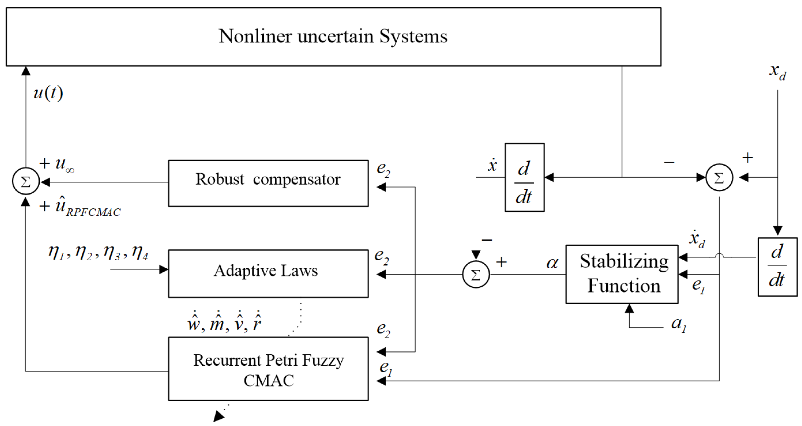
The system can be asymptotically stabilized by the IBC in (7). However, the system functions ($f_0\left(\mathbf{x}\right)$, $g_0$, and $d_0\left(\mathbf{x}\right)$) usually do not exist in their exact forms in practice. Therefore, it is not possible to directly implement the IBC in (10). A recurrent Petri fuzzy CMAC-based robust adaptive backstepping (RPFCRAB) control system, shown in Figure 5, is suggested as a solution to this constraint. The suggested controller’s structure follows

$$u=\widehat{u}+u_{\infty },$$

(18)

where $\widehat{u}$ denotes the recurrent Petri fuzzy CMAC (RPFC) and $u_{\infty }$ represents the $H^{\infty }$ robust compensator.

A novel RPFC is introduced, formulated through the following fuzzy inference rule.

Rule i: If $I_1$ is a member of $f_{1jk}$, $I_2$ is a member of $f_{2jk}$, and $I_3$ is a member of $f_{3jk}$, then $O_{jk}=W_{jk}$, for $j=1,2,\dots ,n_j,k=1,2,\dots ,n_k,$ and $\lambda =1,2,\dots ,n_l$, where $n_i$ is the number of input dimensions, $n_j$ is the number of layers associated with each input dimension, $n_k$ indicates the number of blocks in each layer, and $n_l=n_j{n}_k$ is the total number of fuzzy rules. The fuzzy region connected to the $i^{\mathrm{th}}$ input, $j^{\mathrm{th}}$ layer, and $k^{\mathrm{th}}$ block is defined by the set $f_{ijk}$, while the corresponding weight is indicated by $w_{jk}$. The following figure depicts a schematic of a fuzzy CMAC system with two inputs ($n_i=2$), four layers ($n_j=4$), and two blocks ($n_k=2$) per layer.

The input space, association memory, receptive field, weight memory, and output space are the five primary parts of the RPFC. Below, we provide a succinct description of signal transmission over these spaces.

• Input Space: If $n_i$ is the number of input variables, then each input vector $I={\left[I_1,\dots ,I_i,\dots ,I_{n_i}\right]}^T\in {\mathbb{R}}^{n_i}$ is discretized into regions (referred to as elements or neurons) based on the control domain. The resolution is defined by the number of such elements $n_e$.
• Association Memory (Membership Function): Blocks are created by combining groups of elements together. Every block serves as a framework for a receptive field. The receptive field basis function used in this work is a Gaussian function, which can be written as

  $${\mu }_{ik}\left(i_{ri}\right)=exp\left({\displaystyle \frac{-{\left(i_{ri}-m_{ik}\right)}^2}{v_{ik}}}\right)$$

  (19)

  for $k=1,2,\cdots ,n_b$. Here, ${\mu }_{ik}$ represents the $k^{th}$ block of the $i^{th}$ input $I_i$ with $m_{ik}$ and variance $v_{ik}$. Furthermore, this block’s input can be shown as

  $$i_{ri}=i_{ri}+r_{ik}{\mu }_{ik}\left(t-T\right),$$

  (20)

  where $r_{ik}$ is the recurrent gain and ${\mu }_{ik}\left(t-T\right)\underline{\underline{\mathrm{\Delta }}}{\mu }_{ikT}$ denotes the value of $r_{ik}$ through time delay T. It is evident that the network’s historical data displays a dynamic mapping. This is the clear distinction between the traditional CMAC and the suggested ARPFCMAC. The schematic diagram of a 2D RPFCMAC with $n_E=7$ and $n_C=4$ is shown in Figure 5, where $i_1$ is split into blocks $a_1$ and $b_1$, while $i_2$ is divided into blocks $a_2$ and $b_2$. The number of elements in a full block is denoted by $n_C$. Each variable can be shifted by one element to produce alternative blocks. Examples of potential shifted elements are blocks $c_1$ and $d_1$ for $i_1$ and blocks $c_2$ and $d_2$ for $i_2$. Three parameters can be changed for each block in this area: $m_{ik}$, ${\sigma }_{ik}$, and $r_{ik}$ [32,33].
• Petri Memory Space $P_s$: The Petri memory space follows a learning rule to select suitable fired nodes:

  $$\begin{array}{c}{g}_{i,l}^j=max\_l\left\{\underset{j=1,\cdots ,n_{pi}}{sort}\left[{\alpha }_i^j\left(ne{t}_j\left(I_i\right)\right)\right]\right\}\hfill \\ T_j=\left\{\begin{array}{c}1,g_{i,l}^j={\alpha }_i^j\left(ne{t}_j\left(I_i\right)\right)\hfill \\ 0,otherwise\hfill \end{array}\right.\hfill \end{array}$$

  (21)

  where $T_j$ denotes the transition and $n_d$ is the predetermined fired number.
• Receptive Field ${\phi }_s$: In this study, the receptive field number $n_d$ is identical to $n_b$:

  $$\begin{array}{c}{\phi }_K(\mathbf{I},m_k,{\mathbf{v}}_k,{\mathbf{r}}_k)\hfill \\ =\left\{\begin{array}{c}{\displaystyle \prod _{i=1}^{n_i}}{\mu }_{ik}\left(I_j\right)=exp\left[{\displaystyle \sum _{i=1}^{n_i}}{\displaystyle \frac{-{\left(I_i-m_{ik}\right)}^2}{v_{ik}^2}}\right],T_j=1\hfill \\ 0,T_j=0\hfill \end{array}\right.\hfill \end{array}$$

  (22)

  for $k=1,2,\cdots ,n_d$, where ${\mathbf{m}}_k={\left[m_{1k},m_{2k},\cdots ,m_{n_{i}k}\right]}^T\in R^{n_i}$ and ${\mathbf{v}}_k=\left[v_{1k},v_{2k},\cdots ,\right.$${\left.v_{n_{i}k}\right]}^T\in R^{n_i}$. The vector representation of the multidimensional receptive field functions is as follows:

  $$\mathrm{\Phi }\left(\mathbf{I},\mathbf{m},\mathbf{v},\mathbf{r}\right)={({\phi }_1,\cdots ,{\phi }_k,\cdots ,{\phi }_{n_d})}^T$$

  (23)

  where ${\mathbf{m}}_k={[m_1^T,\cdots ,m_k^T,\cdots ,m_{n_d}^T]}^T\in R^{n_i{n}_d}$ and ${\mathbf{v}}_k={[v_1^T,\cdots ,v_k^T,\cdots ,v_{n_d}^T]}^T\in R^{n_i{n}_d}$.
• Weight Memory Space $w_s$: The expression for each location of $R_s$ with respect to a specific adjustable value in the weight memory space is defined as

  $$\mathbf{w}={[w_1,\cdots ,w_k,\cdots ,w_{n_d}]}^T\in R^{n_d},$$

  (24)

  where $w_j$ represents the output’s connecting weight value for the $n_{th}$ receptive field.
• Output Space $O_s$: The algebraic total of the activated weighted receptive field is the RPFC’s output, which can be written as

  $$u=o={\mathbf{w}}^T\mathrm{\Phi }=\sum _{k=1}^{n_d}{w}_k{\phi }_k.$$

  (25)

3.4. Online Learning Algorithm

The main tracking controller in Equation (25) that is intended to imitate the IBC is the RPFC u. To ensure robust tracking performance, the robust compensator $u_{\infty }$ is introduced to minimize the disparity between the IBC and the RPFC. The relevant parameter adaptation rules for the RPFC will be created later. To make things easier, we can create the vectors $\mathbf{m}$, $\mathbf{v}$, and $\mathbf{i}$ to aggregate all of the RPFC’s parameters as

$$\mathbf{m}={[m_{1jk}^T,\cdots ,m_{ijk}^T,\cdots ,m_{n_{i}jk}^T]}^T\in R^{n_i{n}_j{n}_k},$$

(26)

where

$${\mathbf{m}}_{ijk}=\left[m_{i11},\cdots ,m_{i1n_k},m_{i21},\cdots ,m_{i2n_k},m_{i{n}_{j}1},\cdots ,m_{i{n}_{j}1},\cdots m_{i{n}_j{n}_k}{]}^T\in R^{n_i{n}_k}\right.$$

(27)

and

$$\mathbf{v}={[v_{1jk}^T,\cdots ,v_{ijk}^T,\cdots ,v_{n_{i}jk}^T]}^T\in R^{n_i{n}_j{n}_k},$$

(28)

for which

$${\mathbf{v}}_{ijk}=\left[v_{i11},\cdots ,v_{i1n_k},v_{i21},\cdots ,v_{i2n_k},\right.v_{i{n}_{j}1},\cdots ,v_{i{n}_{j}1},\cdots v_{i{n}_j{n}_k}{]}^T\in R^{n_i{n}_k}$$

(29)

and

$$\mathbf{i}={[i_{1jk}^T,\cdots ,i_{ijk}^T,\cdots ,i_{n_{i}jk}^T]}^T\in R^{n_i{n}_j{n}_k},$$

(30)

where

$${\mathbf{i}}_{ijk}=\left[i_{i11},\cdots ,i_{i1n_k},i_{i21},\cdots ,i_{i2n_k},\right.i_{i{n}_{j}1},\cdots ,i_{i{n}_{j}1},\cdots i_{i{n}_j{n}_k}{]}^T\in R^{n_i{n}_k}.$$

(31)

Assume that there exists an optimal $u^{*}$ to approach the IBC $u_{IBC}^{*}$ such that

$$u_{IBC}^{*}=u^{*}(I,w^{*},m^{*},v^{*},{\psi }^{*})+\epsilon ={\mathbf{w}}^{\ast T}{\mathbf{r}}^{\ast }+\epsilon ,$$

(32)

where $\epsilon$ denotes the minimal reconstruction error and $w^{*}$, $m^{*}$, $v^{*}$, ${\psi }^{*}$, and $r^{*}$ correspond to the optimal parameter matrix and vectors associated with w, m, v, $\psi$, and r, respectively. Because the exact optimal RPFC $u^{*}$ is generally unattainable in practice, an online adaptive estimator of the RPFC is introduced to approximate it. Accordingly, from Equation (25), the control law can be reformulated as

$$u=\widehat{u}+u_{\infty }={\widehat{\mathbf{w}}}^{*}\widehat{\mathbf{r}}+u_{\infty }.$$

(33)

Subtracting (33) from (32), an estimation error $\tilde{u}$ can be obtained as follows:

$$\begin{array}{c}\begin{array}{c}\tilde{u}\equiv u_{IBC}^{*}-u\hfill \\ ={{\mathbf{w}}^{*}}^{\mathrm{T}}{\mathbf{r}}^{*}+\epsilon -\stackrel{\wedge }{\mathbf{w}}T\stackrel{\wedge }{\mathbf{r}}+u_{\infty }\hfill \end{array}\\ ={\tilde{\mathbf{w}}}^T{\mathbf{r}}^{*}+\stackrel{\wedge }{\mathbf{w}}T{\mathbf{r}}^{*}+\epsilon -u_{\infty }\end{array}$$

(34)

where $\tilde{w}=w^{*}-\widehat{w}$ and $\tilde{r}=r^{*}-\widehat{r}$. Because the linearization technique can transform the multidimensional receptive field basis functions into a partially linear form, the expansion of $\tilde{r}$ in a Taylor series can be obtained, i.e.,

$$\begin{array}{c}\tilde{\phi }=\left[\begin{array}{c}{\tilde{\phi }}_1\\ ⋮\\ {\tilde{\phi }}_l\\ ⋮\\ {\tilde{\phi }}_{n_l}\end{array}\right]\hfill \\ ={\left.\left[\begin{array}{c}{\left({\displaystyle \frac{\partial {\phi }_1}{\partial m}}\right)}^T\\ ⋮\\ {\left({\displaystyle \frac{\partial {\phi }_l}{\partial m}}\right)}^T\\ ⋮\\ {\left({\displaystyle \frac{\partial {\phi }_{n_l}}{\partial m}}\right)}^T\end{array}\right]\right|}_{m=\widehat{m}}(m^{*}-\widehat{m})+{\left.\left[\begin{array}{c}{\left({\displaystyle \frac{\partial {\phi }_1}{\partial v}}\right)}^T\\ ⋮\\ {\left({\displaystyle \frac{\partial {\phi }_l}{\partial v}}\right)}^T\\ ⋮\\ {\left({\displaystyle \frac{\partial {\phi }_{n_l}}{\partial v}}\right)}^T\end{array}\right]\right|}_{v=\widehat{v}}(v^{*}-\widehat{v})+{\left.\left[\begin{array}{c}{\left({\displaystyle \frac{\partial {\phi }_1}{\partial \psi }}\right)}^T\\ ⋮\\ {\left({\displaystyle \frac{\partial {\phi }_l}{\partial \psi }}\right)}^T\\ ⋮\\ {\left({\displaystyle \frac{\partial {\phi }_{n_l}}{\partial \psi }}\right)}^T\end{array}\right]\right|}_{\psi =\widehat{\psi }}({\psi }^{*}-\psi )+O_t\hfill \\ ={\mathbf{r}}_m^T\tilde{\mathbf{m}}+{\mathbf{r}}_v^T\tilde{\mathbf{v}}+{\mathbf{r}}_{\psi }^T\tilde{\psi }+{\mathbf{O}}_t,\hfill \end{array}$$

(35)

where $\tilde{m}=m^{*}-\widehat{m}$, $\tilde{v}=v^{*}-\widehat{v}$, $\tilde{i}=i^{*}-\widehat{i}$, and $O_t\in R^{n_l}$ is a vector of higher-order terms. Here, ${\displaystyle \frac{\partial {\phi }_l}{\partial m}}$, ${\displaystyle \frac{\partial {\phi }_l}{\partial v}}$, and ${\displaystyle \frac{\partial {\phi }_l}{\partial \psi }}$ are respectively defined as

$$\left[{\displaystyle \frac{\partial {\phi }_l}{\partial m}}\right]={\left[\underset{(l-1)\times n_i}{\underbrace{0,\dots ,0,}}{\displaystyle \frac{\partial {\phi }_l}{\partial m_{1l}}},\dots ,{\displaystyle \frac{\partial {\phi }_{\mathbf{l}}}{\partial m_{n_{i}l}}}\underset{(n_l-l)\times n_i}{\underbrace{,0,\dots ,0}}\right]}^T,$$

(36)

$$\left[{\displaystyle \frac{\partial {\phi }_l}{\partial v}}\right]={\left[\underset{(l-1)\times n_i}{\underbrace{0,\dots ,0,}}{\displaystyle \frac{\partial {\phi }_{\mathbf{l}}}{\partial v_{1l}}},\dots ,{\displaystyle \frac{\partial {\phi }_l}{\partial v_{n_{i}l}}}\underset{(n_l-l)\times n_i}{\underbrace{,0,\dots ,0}}\right]}^T,$$

(37)

$$\left[{\displaystyle \frac{\partial {\phi }_l}{\partial \psi }}\right]={\left[\underset{(l-1)\times n_i}{\underbrace{0,\dots ,0,}}{\displaystyle \frac{\partial {\phi }_l}{\partial {\psi }_{1l}}},\dots ,{\displaystyle \frac{\partial {\phi }_l}{\partial {\psi }_{n_{i}l}}}\underset{(n_l-l)\times n_i}{\underbrace{,0,\dots ,0}}\right]}^T.$$

(38)

Rewriting (35) yields

$${\mathrm{\Phi }}^{*}=\widehat{\phi }+{\phi }_m^T\tilde{m}+{\phi }_v^T\tilde{v}+{\phi }_{\psi }^T\tilde{\psi }+O_t,$$

(39)

while substituting (35) and (39) into (34) yields

$$\begin{array}{cc}\hfill \tilde{u}& ={\tilde{\mathbf{w}}}^{\mathbf{T}}(\widehat{\phi }+{\phi }_{\mathbf{m}}^{\mathbf{T}}\tilde{\mathbf{m}}+{\phi }_{\mathbf{v}}^{\mathbf{T}}\tilde{\mathbf{v}}+{\phi }_{\psi }^{\mathbf{T}}\tilde{\psi }+{\mathbf{O}}_{\mathbf{t}})+{\widehat{\mathbf{w}}}^{\mathbf{T}}({\phi }_{\mathbf{m}}^{\mathbf{T}}\tilde{\mathbf{m}}+{\phi }_{\mathbf{v}}^{\mathbf{T}}\tilde{\mathbf{v}}+{\phi }_{\psi }^{\mathbf{T}}\tilde{\psi }+{\mathbf{O}}_{\mathbf{t}})+\epsilon -u_{\infty }\hfill \\ & ={\tilde{\mathbf{w}}}^{\mathbf{T}}\widehat{\mathbf{r}}+{\widehat{\mathbf{w}}}^{\mathbf{T}}({\phi }_{\mathbf{m}}^{\mathbf{T}}\tilde{\mathbf{m}}+{\phi }_{\mathbf{v}}^{\mathbf{T}}\tilde{\mathbf{v}}+{\phi }_{\psi }^{\mathbf{T}}\tilde{\psi })+\xi \left(t\right)-u_{\infty },\hfill \end{array}$$

(40)

where the approximation error is expressed as $\xi \left(t\right)={\tilde{w}}^T{\phi }_m^T\tilde{m}+{\tilde{w}}^T{\phi }_v^T\tilde{v}+{\tilde{w}}^T{\phi }_{\psi }^T\tilde{\psi }+{w^{*}}^T{O}_t+\epsilon$. Then, Equation (7) can be expressed via (10) into (9) and (38) as

$${\dot{e}}_2=g_0[{\tilde{w}}^T\widehat{\phi }+{\tilde{w}}^T({\phi }_m^T\tilde{m}+{\phi }_v^T\tilde{v}+{\phi }_{\psi }^T\tilde{\psi })+\xi \left(t\right)]-u_{\infty }-e_1-k_2{e}_2.$$

(41)

Although ARPFC is applied to approximate the IBC, the presence of approximation errors prevents direct assurance of system stability. To address this issue, a robust compensator $u_{\infty }$ is introduced to counteract the approximation uncertainty and ensure robust stability of the closed-loop system. When $\xi \left(t\right)$ is present, a prescribed $H_{\infty }$ tracking performance is considered, as in [28]:

$$\begin{array}{c}\hfill {\int }_0^T{e}_2^2\left(t\right)dt\le {\displaystyle \frac{e_1^2\left(0\right)}{g_0}}+{\displaystyle \frac{e_2^2\left(0\right)}{g_0}}+{\displaystyle \frac{1}{l_1}}{\tilde{w}}^T\left(0\right)\tilde{w}\left(0\right)+{\displaystyle \frac{1}{l_2}}{\tilde{m}}^T\left(0\right)\tilde{m}\left(0\right)\\ \hfill +{\displaystyle \frac{1}{l_3}}{\tilde{v}}^T\left(0\right)\tilde{v}\left(0\right)+{\displaystyle \frac{1}{l_4}}{\tilde{\psi }}^T\left(0\right)\tilde{\psi }\left(0\right)+{\delta }^2{\int }_0^T{\xi }^2\left(t\right)dt\end{array}$$

(42)

where $l_1$, $l_2$, $l_3$, and $l_4$ are positive learning rates and $\xi \left(t\right)$ denotes a disturbance or prescribed attenuation signal associated with $e_2\left(t\right)$. Assuming that the system is initialized with $e_1\left(0\right)=0$, $e_2\left(0\right)=0$, $\tilde{w}\left(0\right)=0$, $\tilde{m}\left(0\right)=0$, $\tilde{v}\left(0\right)=0$, and $\tilde{\psi }\left(0\right)=0$, under these conditions the $H\infty$ tracking criterion in (42) can be expressed as

$$\underset{\xi \left(t\right)\in L_2[0,T]}{sup}{\displaystyle \frac{{\parallel e_2\left(t\right)\parallel }_{L_2}}{{\parallel \xi \left(t\right)\parallel }_{L_2}}}\le \delta ,$$

(43)

where ${\parallel e_2\left(t\right)\parallel }_{L_2}^2={\int }_0^T{e}_2^2\left(t\right),dt$ and ${\parallel \xi \left(t\right)\parallel }_{L_2}^2={\int }_0^T{\xi }^2\left(t\right),dt$. This inequality indicates that $\delta$ characterizes the attenuation ratio between the uncertainty $\xi \left(t\right)$ and the output error $e_2\left(t\right)$. In the limiting case $\delta =\infty$, the condition corresponds to pure tracking control without any attenuation of approximation errors [28]. Consequently, the following theorem can be established.

Theorem 1.

Consider the magnetic levitation system described by (2). Suppose that the ARPFC control scheme is specified by (33), with its parameter adaptation updated through (44)–(47), and that robust compensation is constructed as in (47). Under these conditions, the closed-loop dynamics satisfy the robust performance criterion (42) for the chosen attenuation level δ.

$$\dot{\widehat{\mathbf{w}}}=l_1{e}_2\left(t\right)\widehat{\phi }$$

(44)

$$\dot{\widehat{\mathbf{m}}}=l_2{e}_2\left(t\right){\phi }_{\mathbf{m}}\widehat{\mathbf{w}}$$

(45)

$$\dot{\widehat{\mathbf{v}}}=l_3{e}_2\left(t\right){\phi }_{\mathbf{v}}\widehat{\mathbf{w}}$$

(46)

$$\dot{\widehat{\psi }}=l_4{e}_2\left(t\right){\phi }_{\psi }\widehat{\mathbf{w}}$$

(47)

$$u_{\infty }={\displaystyle \frac{{\delta }^2+1}{2{\delta }^2}}{e}_2\left(t\right)$$

(48)

Proof. 

The Lyapunov function candidate is provided by

$$V_2=V_1+{\displaystyle \frac{g_0}{2l_1}}{\tilde{w}}^T\tilde{w}+{\displaystyle \frac{g_0}{2l_2}}{\tilde{m}}^T\tilde{m}+{\displaystyle \frac{g_0}{2l_3}}{\tilde{v}}^T\tilde{v}+{\displaystyle \frac{g_0}{2l_4}}{\tilde{\psi }}^T\tilde{\psi }.$$

(49)

Taking the derivative of the Lyapunov function and using (41) yields

$$\begin{array}{c}{\dot{V}}_2={\dot{V}}_1+{\displaystyle \frac{g_0}{l_1}}{\tilde{w}}^T\dot{\tilde{w}}+{\displaystyle \frac{g_0}{l_2}}{\tilde{m}}^T\dot{\tilde{m}}+{\displaystyle \frac{g_0}{l_3}}{\tilde{v}}^T\dot{\tilde{v}}+{\displaystyle \frac{g_0}{l_4}}{\tilde{\psi }}^T\dot{\tilde{\psi }}\hfill \\ =-k_1{e}_1^2\left(t\right)+e_1\left(t\right)e_2\left(t\right)+e_2\left(t\right)\left\{g_0\right[{\tilde{w}}^T\widehat{r}+{\widehat{w}}^T({\phi }_m^T\tilde{m}+{\phi }_v^T\tilde{v}+{\phi }_{\psi }^T\tilde{\psi })+\xi \left(t\right)-u_{\yen }]\hfill \\ -e_1-k_2{e}_2\}+{\displaystyle \frac{g_0}{l_1}}{\tilde{w}}^T\dot{\tilde{w}}+{\displaystyle \frac{g_0}{l_2}}{\tilde{m}}^T\dot{\tilde{m}}+{\displaystyle \frac{g_0}{l_3}}{\tilde{v}}^T\dot{\tilde{v}}+{\displaystyle \frac{g_0}{l_4}}{\tilde{\psi }}^T\dot{\tilde{\psi }},\hfill \end{array}$$

(50)

where ${\widehat{w}}^T{\phi }_m^T\tilde{m}=\tilde{m}{\phi }_m\widehat{w}$, ${\widehat{w}}^T{\phi }_v^T\tilde{v}=\tilde{m}{\phi }_v\widehat{v}$, and ${\widehat{w}}^T{\phi }_{\psi }^T\tilde{\psi }=\tilde{m}{\phi }_{\psi }\widehat{\psi }$ are used because they are scales. Then, (50) can be rewritten as

$$\begin{array}{c}\begin{array}{c}{\dot{V}}_2=-k_1{e}_1^2\left(t\right)-k_2{e}_2^2\left(t\right)+g_0{\tilde{w}}^T[e_2\left(t\right)\widehat{\phi }-{\displaystyle \frac{1}{l_1}}\dot{\widehat{w}}]\hfill \\ +g_0{\tilde{m}}^T[e_2\left(t\right){\phi }_m\widehat{w}-{\displaystyle \frac{1}{l_2}}\dot{\widehat{m}}]+g_0{\tilde{v}}^T[e_2\left(t\right){\phi }_v\widehat{w}-{\displaystyle \frac{1}{l_3}}\dot{\widehat{v}}]\hfill \end{array}\hfill \\ +g_0{\tilde{\psi }}^T[e_2\left(t\right){\phi }_{\psi }\widehat{w}-{\displaystyle \frac{1}{l_1}}\dot{\widehat{\psi }}]+g_0{e}_2\left(t\right)\xi \left(t\right)-g_0{e}_2\left(t\right)u_{\infty }.\hfill \end{array}$$

(51)

From (44) and (47), we can use (48) to rewrite Equation (49) as

$$\begin{array}{c}{\dot{V}}_2=-k_1{e}_1^2\left(t\right)-k_2{e}_2^2\left(t\right)+g_0{e}_2\left(t\right)\xi \left(t\right)-g_0{e}_2\left(t\right){\displaystyle \frac{{\delta }^2+1}{2{\delta }^2}}{e}_2\left(t\right)\hfill \\ \begin{array}{c}=-k_1{e}_1^2\left(t\right)-k_2{e}_2^2\left(t\right)-{\displaystyle \frac{1}{2}}{g}_0{e}_2^2\left(t\right)-{\displaystyle \frac{1}{2}}{g}_0{[{\displaystyle \frac{e_2\left(t\right)}{\delta }}-\delta \xi \left(t\right)]}^2+{\displaystyle \frac{1}{2}}{g}_0{\delta }^2{\xi }^2\left(t\right)\hfill \\ \le -{\displaystyle \frac{1}{2}}{g}_0{e}_2^2\left(t\right)+{\displaystyle \frac{1}{2}}{g}_0{\delta }^2{\xi }^2\left(t\right).\hfill \end{array}\hfill \end{array}$$

(52)

Assuming $\xi \left(t\right)\in L_2[0,T]$, $\forall T\in [0,\infty ]$, integrating the above equation from $t=0$ yields

$$V_2\left(T\right)-V_2\left(0\right)\le -{\displaystyle \frac{1}{2}}{g}_0{\int }_0^T{e}_2^2\left(t\right)dt+{\displaystyle \frac{1}{2}}{g}_0{\delta }^2{\int }_0^T{\xi }^2\left(t\right)dt.$$

(53)

Because $V_2\left(T\right)\ge 0$, the above inequality implies the inequality

$${\displaystyle \frac{1}{2}}{g}_0{\int }_0^T{e}_2^2\left(t\right)dt\le V_2\left(0\right)+{\displaystyle \frac{1}{2}}{g}_0{\delta }^2{\int }_0^T{\xi }^2\left(T\right)dt.$$

(54)

Using (49), this inequality is shown to be equivalent to (42); thus, the proof is completed. Accordingly, the detailed design procedure can be summarized by the block diagram in Figure 5. Specifically, the error signals $e_1\left(t\right)$ and $e_2\left(t\right)$ are first obtained from (4)–(6). Next, the adaptive parameter update laws derived in (44)–(47) are applied and the recurrent Petri fuzzy CMAC is constructed according to (35). Finally, to ensure the convergence of the tracking error, the approximation error term $\xi \left(t\right)$ must belong to $L_2[0,T]$. Moreover, the learning rates $l_1$, $l_2$, $l_3$, and $l_4$ in (44)–(47) should be selected empirically through trial and adjustment.

The purpose of the online learning mechanism in the proposed CMAC structure is not to carry out full-scale reinforcement learning or dynamic programming, but rather to perform localized incremental adaptation during runtime. The update rule in (34) only requires current tracking error and receptive field activation information, resulting in constant-time updates with negligible computational burden. This design permits the controller to refine its performance in the presence of varying disturbances or modeling uncertainties without the need to engage in the game-theoretic policy iteration required by recent safe reinforcement learning approaches [41,42]. Consequently, the proposed online learning scheme offers improved robustness while maintaining real-time applicability. □

3.5. BCMO Algorithm

The balancing composite motion optimization (BCMO) algorithm balances global and local search mechanisms to efficiently find optimal solutions. In order to find the optimal parameters $l_1$, $l_2$,$l_3$, and $l_4$, let x represent the set of them, i.e., $x=l_1,l_2,l_3,l_4$.

The following equation is used to uniformly initialize the population distribution in the solution space during the first generation:

$$x_i=x_i^L+rand(1,d)(x_i^U-x_i^L)$$

(55)

where $rand$ is a d-dimensional vector that satisfies uniform distribution in the interval [0,1], while $x_i^L$ and $x_i^U$ represent the lower and upper bounds of the $i^{th}$ individual, respectively.

The following formula can be used to determine the $i^{th}$ individual’s motion vector in each generation with regard to the overall optimal point, represented as $v_i$:

$$v_i=v_{i/j}+v_j$$

(56)

where $v_i$ and $v_j$ are the movement vectors of the $i^{th}$ and $j^{th}$ individuals with respect to O, respectively, and $v_{i/j}$ is the relative movement vector of the $i^{th}$ individual with regard to the $j^{th}$ individual. The alternative overall optimal score, represented by $O_{in}$, can be determined using the following formula:

$$x_{O_{in}}^t=\left\{\begin{array}{c}{x}_1^t,\mathrm{If}f\left(x_i^t\right)<f\left(x_i^{t-1}\right)\hfill \\ x_1^{t-1},\mathrm{otherwise}.\hfill \end{array}\right.$$

(57)

The best individual in the current generation $u_1^t$ is determined using the population data from the previous generation:

$$u_1^t={\displaystyle \frac{LB-UB}{2}}+v_{k1/k2}^t+v_{k2/k1}^t$$

(58)

where the search space’s lower and upper bounds are denoted by $LB$ and $UB$, respectively, while the relative pseudo-movements of the $k_1^{th}$ individual in relation to the $k_2^{th}$ individual and of the $k_2^{th}$ individual in relation to the previous best individual are denoted by $v_{k1/k2}^t$ and $v_{k2/k1}^t$, respectively. Here, $k_1$ is chosen at random from the range of [2, NP] and $k_2<k_1$, where NP is the number of individuals in the population. Lastly, the following formula determines the $i^{th}$ individual’s position in the subsequent generation:

$$x_i^{i+1}=x_i^t+v_{i/j}+v_j.$$

(59)

The objective function is chosen as $F=e^2$, where e represents the error, in order to minimize the trajectory tracking error. The values of 0 and 500 are selected as the bottom and upper bounds, respectively. The maximum number of generations is 100000. The number of individuals is 100000. The CPU time is 3.32 s, and the optimization dimension is 4.

4. Numerical Simulation and Experimental Results

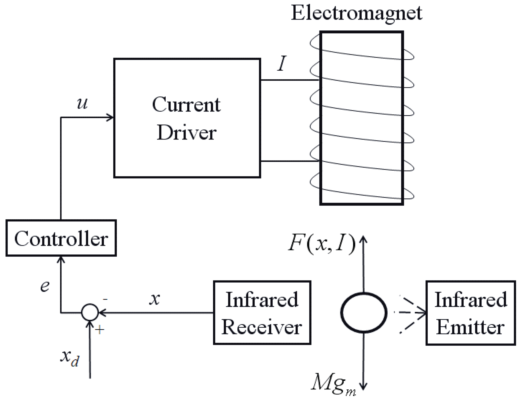
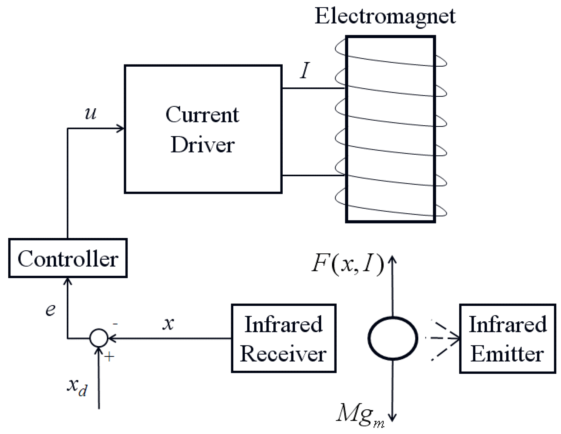
Example 1.

The mechanism for single-axis magnetic levitation is shown in Figure 6. The current driver transforms the voltage signal that serves as the control input into current. The electromagnet is excited by this current, which creates the appropriate magnetic field nearby. An infrared sensor measures the metallic sphere’s position as it travels down the electromagnet’s vertical axis.

The specifications of MLS is $N=2850$, $r_1=0.012\left(\mathrm{m}\right)$, $r_2=0.038\left(\mathrm{m}\right)$, $A=0.005515\left({\mathrm{m}}^2\right)$, ${\mu }_0=4\pi ·10^{-7}\left(\mathrm{Wb}/\mathrm{Am}\right)$, $M=0.0216\left(\mathrm{kg}\right)$, $g_m=9.8(\mathrm{m}/{\mathrm{s}}^2)$, $h=0.065\left(\mathrm{m}\right)$, and $\delta x=0.0265\left(\mathrm{m}\right)$.

The constant learning rates for the CMAC controller are $l_w=10$, $l_m=l_v=0.5$. The threshold value settings for the DPFNN controller are set to $l_m=l_v=0.5$, $b=10$, and $c=10$. To achieve sufficient control performance and meet stability requirements across a variety of operating situations, the initial values were chosen by running a genetic algorithm on the offline model. These parameters are then usually adjusted and improved through a trial-and-error procedure. Smaller learning rate values often make parameter convergence easier, but sacrifice learning efficiency in the process. On the other hand, learning proceeds more quickly if the learning rates is set high; however, the proposed control mechanism can become unstable if the parameters change. The metallic sphere is initially positioned at −1 mm. 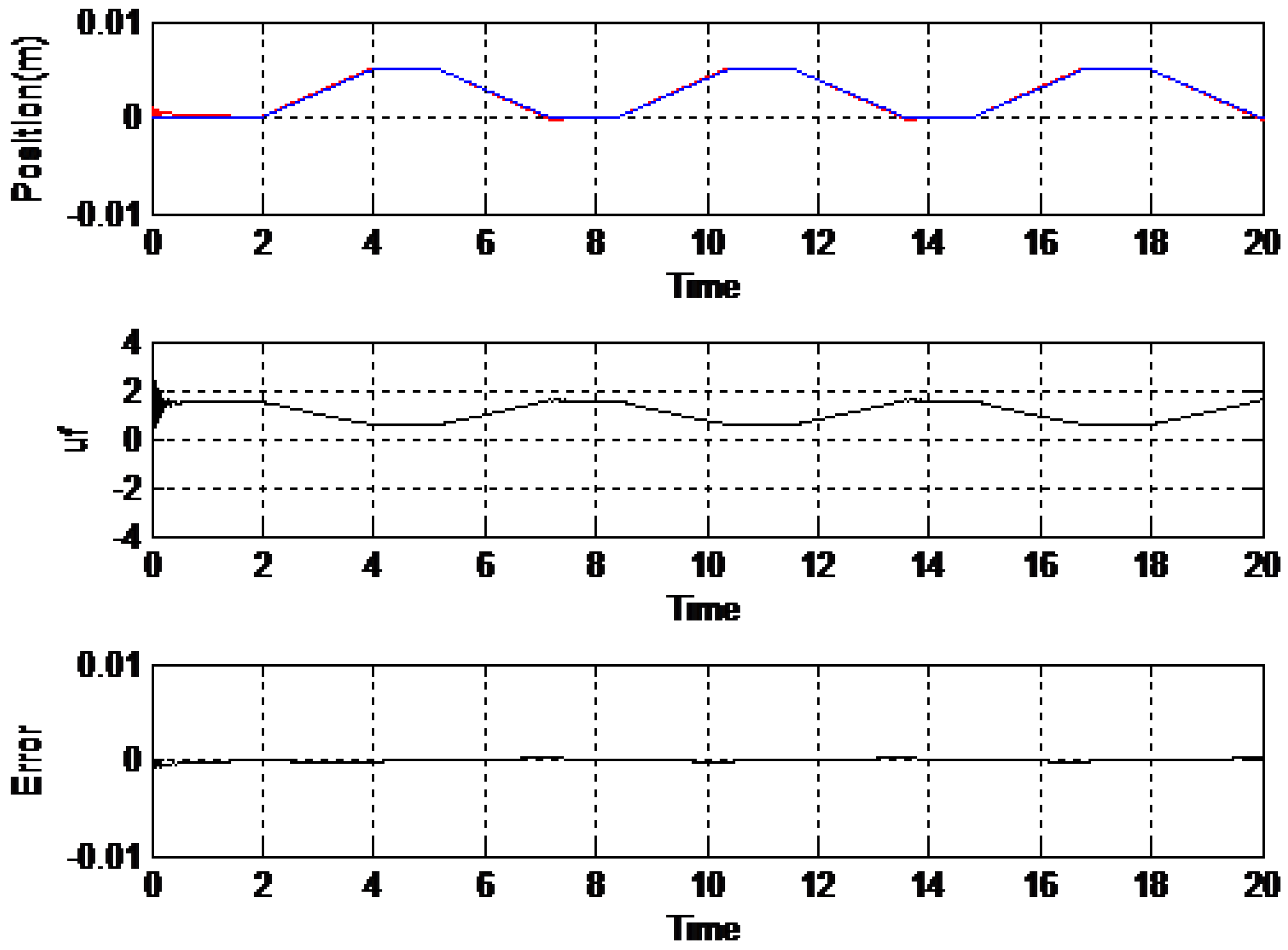Figure 7 displays the CMAC controller’s results, while Figure 8 displays the DPFNN controller’s results.

As shown in the Figure 7, the CMAC controller struggles with position tracking, particularly at the peaks and valleys of the reference trajectory, leading to noticeable tracking errors. These errors are evidenced by the red dashed line deviating from the blue reference line, indicating that the CMAC controller is less precise in following the desired trajectory. Additionally, the control signal ($uf$) associated with the CMAC controller exhibits significant oscillations and fluctuations, reflecting a higher control effort and potential instability. This suggests inefficiency in the control process, as the controller must work harder to maintain performance, yet still results in substantial errors.

In contrast, the DPFNN controller depicted in the second image demonstrates a marked improvement in both tracking accuracy and error minimization. The red dashed line closely follows the blue reference line, with reduced deviations indicating lower tracking errors and a more precise response to the desired trajectory. The control signal for the DPFNN controller is also noticeably more stable and exhibits fewer oscillations compared to the CMAC controller. This reduced fluctuation suggests that the DPFNN controller requires less control effort, enhancing overall efficiency and stability.

In terms of error, the DPFNN controller significantly outperforms the CMAC controller by maintaining lower error margins throughout the trajectory. Its improved accuracy and reduced control effort make the DPFNN controller a more robust and effective solution, particularly in scenarios requiring precise and stable control. Overall, the DPFNN controller’s superior performance in minimizing errors and enhancing control efficiency underscores its advantage over the traditional CMAC controller.

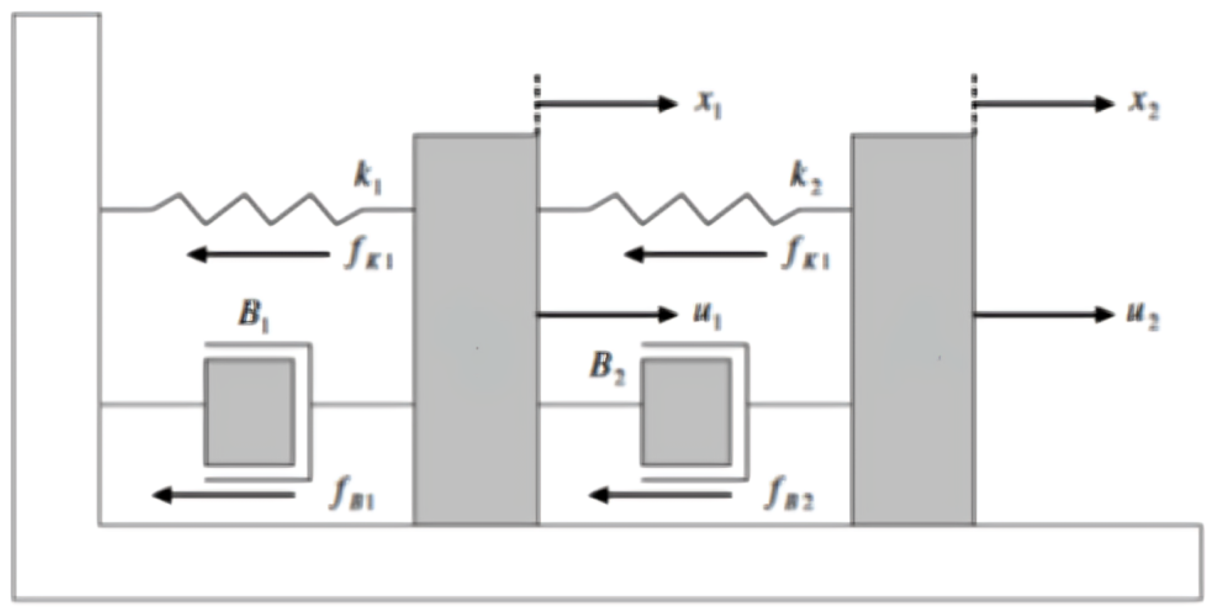
Example 2.

A mass–spring–damper mechanical system

Figure 9 depicts a mass–spring–damper mechanical system. This mechanical system’s dynamic equations are written as follows:

$${\tau }_1{\ddot{x}}_1\left(t\right)=-f_{K1}\left(x\right)-f_{B1}\left(x\right)+f_{K2}\left(x\right)+f_{B2}\left(x\right)+u_1\left(t\right)+\mathrm{\Delta }{u}_{12}\left(t\right)+{\delta }_1\left(t\right)$$

(60)

$${\tau }_2{\ddot{x}}_2\left(t\right)=-f_{K2}\left(x\right)-f_{B2}\left(x\right)+u_2+\mathrm{\Delta }{u}_{21}+{\delta }_2\left(t\right)$$

(61)

where ${\tau }_1$ and ${\tau }_2$ are the masses in the system and $x\left(t\right)={[x_1\left(t\right),x_2\left(t\right),{\dot{x}}_1\left(t\right),{\dot{x}}_2\left(t\right)]}^T$ are the mechanical system’s locations and velocities. The spring forces are $f_{K2}\left(\underline{x}\right)=k_{20}(x_2-x_1)+\mathrm{\Delta }{k}_2{(x_2-x_1)}^3$ and $f_{K2}\left(\underline{x}\right)=k_{20}(x_2-x_1)+\mathrm{\Delta }{k}_2{(x_2-x_1)}^3$, while the frictional forces are $f_{B1}\left(x\right)=b_{10}{\dot{x}}_1+\mathrm{\Delta }{b}_1{\dot{x}}_1^2$ and $f_{B2}\left(x\right)=b_{20}({\dot{x}}_2-{\dot{x}}_1)+\mathrm{\Delta }{b}_2{({\dot{x}}_2-{\dot{x}}_1)}^2$. The parameters for the system are provided as ${\tau }_1=1$, ${\tau }_2=0.8$, $k_{10}=3$, $k_{20}=4$, $b_{10}=2$, $b_{20}=2.2$, $\mathrm{\Delta }{k}_1=0.5$, $\mathrm{\Delta }{k}_2=0.5$, $\mathrm{\Delta }{b}_1=0.5$, $\mathrm{\Delta }{b}_2=0.5$, $\mathrm{\Delta }{u}_{12}=0.2u_2$, $\mathrm{\Delta }{u}_{21}=0.25u_1$, $d_1\left(t\right)=2\exp (-0.2t)$, and $d_2\left(t\right)=-2\exp (-0.1t)$.

Thus, the mass–spring–damper mechanical system’s dynamic equation can be reformulated as follows:

$$\ddot{\mathbf{x}}\left(t\right)=\mathbf{f}\left(\underline{x}\right)+\mathbf{G}\left(\underline{x}\right)\mathbf{u}\left(\mathrm{t}\right)+\mathbf{d}\left(t\right)$$

(62)

where

$$f\left(\underline{x}\right)=\left[{\displaystyle \frac{-f_{K1}\left(\underline{x}\right)-f_{B1}\left(\underline{x}\right)+f_{K2}\left(\underline{x}\right)+f_{B2}\left(\underline{x}\right)}{{\tau }_1}},\right.\left.{\displaystyle \frac{-f_{K2}\left(\underline{x}\right)-f_{B2}\left(\underline{x}\right)}{{\tau }_2}}\right],$$

(63)

in which $G\left(\underline{x}\right)=\left[\begin{array}{cc}{\displaystyle \frac{1}{{\tau }_1}}& {\displaystyle \frac{0.2}{{\tau }_1}}\\ {\displaystyle \frac{0.25}{{\tau }_2}}& {\displaystyle \frac{1}{{\tau }_2}}\end{array}\right]$, $u\left(t\right)\underline{\underline{\mathrm{\Delta }}}{[u_1\left(t\right),u_2\left(t\right)]}^T$ denotes the control input, and $d\left(t\right)\underline{\underline{\mathrm{\Delta }}}{\left[{\displaystyle \frac{d_1\left(t\right)}{{\tau }_1}},{\displaystyle \frac{d_2\left(t\right)}{{\tau }_2}}\right]}^T$ denotes the external disturbance. The outputs of the reference model provide the intended trajectories, while ${\ddot{x}}_{di}\left(t\right)=-16x_{di}\left(t\right)-4{\dot{x}}_{di}\left(t\right)+12r_i$, $i=1,2$ is the chosen reference model. The initial conditions for the mechanical system and reference model are provided as $x_1\left(0\right)=1$, ${\dot{x}}_1\left(0\right)=0$, $x_2\left(0\right)=1$, ${\dot{x}}_2\left(0\right)=0$, $x_{d1}\left(0\right)=0$, $x_{d2}\left(0\right)=0$, ${\dot{x}}_{d1}\left(0\right)=0$, and ${\dot{x}}_{d2}\left(0\right)=0$. The control parameters are selected as $k_1=\left[\begin{array}{cc}0.01& 0\\ 0& 0.01\end{array}\right]$, $c_q=0.8$, $q=1,2,3$, $l_z=0.3$, $l_w=0.01$, $l_m=0.2$, $l_v=0.2$, $\varsigma =1.1$, and $\xi =1.5$, whereas the remaining parameters are all random. The inputs used as references are $r_1={\displaystyle \frac{\pi }{3}}(0.9sin\left({\displaystyle \frac{t}{2}}\right)+0.1sin\left(2t\right))$ and $r_2=\pi (0.4sin\left(t\right)+0.1sin\left(3t\right))$.

The FNN control method, as depicted in Figure 10, is applied to the mass–spring–damper system shown in Figure 9. This system involves two masses connected by springs and dampers, where $x_1$ and $x_2$ represent the positions of the first and second masses, respectively. The FNN control method attempts to regulate the positions $x_1$ and $x_2$ in order to follow the desired trajectories $x_{d1}$ and $x_{d2}$. The response of the system under FNN control shows some oscillations and a phase lag between the actual positions and the desired trajectories. As illustrated in Figure 10A,B, the tracking errors for $x_1$ and $x_2$ exhibit initial offsets and gradually converge, but stabilize around a slightly negative value (approximately −0.5). This indicates that while the FNN method is capable of reducing the tracking error, it cannot achieve perfect tracking, particularly in the steady state. Persistent steady-state errors result from this method’s difficulties in handling the dynamics of the system and external impacts.

The proposed control method, as illustrated in Figure 10, demonstrates a significant improvement in controlling the mass–spring–damper system. Positions $x_1$ and $x_2$ closely follow their desired trajectories $xd1$ and $xd2$, with minimal oscillations and rapid convergence to the desired state. The tracking errors for $x_1$ and $x_2$, shown in Figure 10E,F, are the smallest among the three methods, with errors converging close to zero and stabilizing around −0.1. This performance highlights the proposed controller’s superior accuracy and stability, effectively minimizing the effects of external disturbances and inherent system dynamics. The rapid error convergence and sustained low error levels underscore the capability to deliver precise and reliable control, outperforming both the FNN and CMAC methods. Thus, the proposed method proves highly effective for applications requiring stringent control accuracy and robustness in dynamic environments.

Table 1. Comparison with other methods using RMSE.

	RMSE for x1	RMSE for x2
NN	0.2025	0.2061
CMAC	0.1525	0.1884
Proposed method	0.1308	0.1673

shows a comparison of RMSE between NN, CMAC, and the proposed method for $x1$ and $x2$. The proposed method has the lowest RMSE values for both $x1$ and $x2$, indicating that it provides the best performance in minimizing errors among the three methods.

5. Conclusions

In this paper, we have successfully implemented a CMAC controller for a magnetic levitation system. The proposed DPFNN controller is configured in the absence of intensive computation and inherits the advantages of CMAC controllers, including reduced computational burden during parameter learning. Adaptive tuning principles are employed to accurately eliminate the approximation error. By updating the control parameters according to these laws, satisfactory control performance can be achieved. Additionally, a field-programmable gate array (FPGA) chip serves as the foundation for implementing the designed intelligent controller. The design objectives of small size, low cost, rapid execution speed, and increased flexibility can all be met by implementing the proposed control system with an FPGA chip. Simulation and experimental results for the magnetic levitation system demonstrate the superior control performance and efficacy of the proposed intelligent controller.